marginparsep has been altered.
topmargin has been altered.
marginparwidth has been altered.
marginparpush has been altered.
The page layout violates the ICML style.
Please do not change the page layout, or include packages like geometry,
savetrees, or fullpage, which change it for you.
We’re not able to reliably undo arbitrary changes to the style. Please remove
the offending package(s), or layout-changing commands and try again.
SHAPE: An Unified Approach to Evaluate the Contribution and Cooperation of Individual Modalities
Pengbo Hu * 1 2 Xingyu Li * 2 Yi Zhou 3 2
Abstract
As deep learning advances, there is an ever-growing demand for models capable of synthesizing information from multi-modal resources to address the complex tasks raised from real-life applications. Recently, many large multi-modal datasets have been collected, on which researchers actively explore different methods of fusing multi-modal information. However, little attention has been paid to quantifying the contribution of different modalities within the proposed models. In this paper, we propose the SHapley vAlue-based PErceptual (SHAPE) scores that measure the marginal contribution of individual modalities and the degree of cooperation across modalities. Using these scores, we systematically evaluate different fusion methods on different multi-modal datasets for different tasks. Our experiments suggest that for some tasks where different modalities are complementary, the multi-modal models still tend to use the dominant modality alone and ignore the cooperation across modalities. On the other hand, models learn to exploit cross-modal cooperation when different modalities are indispensable for the task. In this case, the scores indicate it is better to fuse different modalities at relatively early stages. We hope our scores can help improve the understanding of how the present multi-modal models operate on different modalities and encourage more sophisticated methods of integrating multiple modalities.
1 Introduction
The present deep learning algorithms thrive on a wide spectrum of real-life tasks, such as those in the fields of computer vision and natural language processing, for which the essence is to learn the underlying distribution from the dataset. Inspired by these achievements, researchers march on to conquer the more complex tasks that put emphasis on reasoning and knowledge. One character of these complex tasks is that they normally involve data from distinct modalities. For example, in the Visual Question Answering (VQA) task, one must answer the questions based on the knowledge extracted from the corresponding image Goyal et al. (2017); Antol et al. (2015). The ability to fuse multi-modal information serves as the cornerstone to developing solutions to those complex tasks, and it presents severe challenges to the deep learning community.
Recently, many large multi-modal datasets have been collected, e.g. Vadicamo et al. (2017); Zadeh et al. (2018); Bowman et al. (2015); Liang et al. (2021), laying the ground for exploring sophisticated fusion strategies. Beyond the naive methods of early and late fusion strategies, increasing attention has been paid to developing and practicing hybrid fusing strategies Wang (2021); Baltrušaitis et al. (2018); Wang et al. (2020); Bai et al. (2021). Those efforts constantly push forward the model performance on the multi-modal datasets. Despite the success, people gradually realize a subtle limitation of the present progresses: the model performance is almost solely judged on their prediction accuracy. A higher accuracy does not necessarily translate to the better usage of multi-modal information. For example, in the CMU-MOSEI datasets, the accuracy of a unimodal model trained on the text modality is very close to the ones of SOTA multi-modal models Zadeh et al. (2018); Delbrouck et al. (2020). Consequently, there is an urgent need for a quantitative metric that can capture how the underlying models operate on the multi-modal information.
To evaluate the individual modalities’ importance, Gat et al. (2021) proposed the perceptual score, which estimates the contribution of a modality with its marginal performance gain at the presence of other modalities. However, this score cannot measure cross-modal cooperation and, in the presence of more than two modalities, its attribution of the importance to individual modalities does not correctly reflect their marginal contribution. To address the above issues, we draw inspirations from the game theory and propose the SHapley vAlue-based PErceptual (SHAPE) scores to directly evaluate the marginal contribution and the cooperation of individual modalities. The validity of the SHAPE scores roots in the properties of the celebrated Shapley value Shapley (1953). With the SHAPE scores, we aim at providing additional perspectives for evaluating the performance of the multi-modal models, which in turn would help building sophisticated fusion strategies.
Our contributions are three-fold:
-
1.
We propose the SHAPE scores, which are theoretically guaranteed to quantify the marginal contribution of individual modalities and the cross-modal cooperation.
-
2.
With the SHAPE scores, we systematically evaluate the usage of multi-modal information by models using different fusion methods on the different multi-modal datasets for different tasks.
-
3.
We extend the perceptual score to a more informative fine-grained version. Moreover, we demonstrate that the perceptual score implicitly measures the correlation among modalities within the dataset.
2 Related Work
2.1 Multi-modal Fusion Method
The fusion strategies can be roughly classified as early fusion, late fusion, and hybrid fusion Baltrušaitis et al. (2018). In the early fusion, one directly concatenates inputs from individual modalities to build a unified input embedding. In this case, a single pathway model is enough to make a prediction, making the training pipeline easier Kiela et al. (2019). The late fusion usually processes individual modalities in different pathways. The fusion operation is typically implemented on the output from each pathway. The later fusion strategy ignores the low-level feature interaction, making it hard to learn the joint representation of modalities. However, in practice, later fusion enables a model using the different pre-trained models for different pathways, making it more flexible than the early fusion Rodrigues Makiuchi et al. (2019). Hybrid fusion has no specific recipe. The different modalities can be integrated at different stages, on different feature levels, and among different modules. It could effectively promote collaboration among individual modalities. Generally, the optimal hybrid fusion strategy depends on the type of the underlying task. For example, in the VQA task, the co-attention-based fusion methods are proved to be better than other strategies Liu et al. (2019).
2.2 Modality Contribution Attribution
Presently, most evaluation works focus on the feature importance. For example, Lundberg & Lee (2017) proposed the SHapley Additive exPlanations (SHAP) value, which can estimate feature importance using an approximation of the features Shapley values. For evaluating modal importance, Hessel & Lee (2020) adopted an indirect attribution method. They designed a tool called the empirical multimodally-additive function projection (EMAP), which is an effective modal that elimates the cross-modal cooperation in the reference multi-modal model. Through comparing the performance of the reference multi-modal model and its EMAP, one could estimate how much the cross-modal cooperation contribute.
The work most relevant to ours is the perceptual score, which is proposed by Gat et al. (2021) to assess the importance of a modality in the input data for a given model. They adopted a permutation-based approach for removing the modality influence. Specifically, let denote the feature of target modality in the input data point. In order to remove ’s influence, is substituted with a randomly chosen one from another data point, i.e., . The resulting classifier on the permutated data is called the permuted classifier. The perceptual score for is defined as the normalized difference between the accuracies of the normal classifier and the corresponding permutated classifier.
It is worth noting that the perceptual score does not account for the marginal contribution of the target modality . Instead, it measures the ’s contribution conditioned on all other modalities in the dataset. The two types of contributions are the same only in the two-modal case. In the presence of more modalities, it requires a more sophisticated method to compute the marginal contribution. Moreover, there still lacks a quantitative method that isolates the cooperation between different modalities.
2.3 Shapley Value
The Shapley value Shapley (1953) was initially proposed in the coalitional game theory for fair attribution of payouts among the players depending on their contribution to the total payout. A multi-player game is usually defined as a real-valued utility function on its participants. Let denote the set of players in the game. The player can form different coalitions (i.e., subsets of ) whose net effect can be either cooperative or competing. Consider a player and a subset , the marginal contribution of to can be evaluated by
Since a player can interact with any other players, in order to evaluate the marginal contribution of in the game one needs to average over all possible . This is exactly how the Shapley value is defined,
A fair attribution of payouts is considered to satisfy the properties of Efficiency, Symmetry, Dummy and Additivity, and the Shapley value is the only attribution method that has those four properites Molnar (2020). More precisely,
Efficiency
All the individual rewards sum to the overall net payouts, i.e., , where indicates the baseline reward without any player.
Symmetry
If two palyers contribute equally to all possible coalitions, i.e., , then they have the same reward, .
Dummy
A dummy player , which does not contribute to any coalition, i.e., , has the reward as if playing alone, .
Additivity
Consider a combined game , its reward is the sum of the rewards for individual games, i.e. .
Those four properties in turn could be viewed as axioms defining a fair attribution method, and it has been proved that they uniquely lead to the definition of the Shapley value Weber (1988).
3 Method
3.1 Models for Comparison
In deep learning, diverse fusion methods have been developed to address the multi-modal learning tasks Baltrušaitis et al. (2018); Wang (2021). Among them, the Early Fusion and Late Fusion strategies are widely recognized. Besides these two, the rest methods cannot be easily categorized. Depending on specific implementation, the fusion may happen at one particular stage or at multiple stages. In addition, different works usually adopt distinct network architectures, making it infeasible to compare them on the same ground.
The present work is devoted to evaluate the contribution and cooperation of individual modalities under different fusion methods on different multi-modal datasets for different tasks. To achieve this goal, we need (i) a common network architecture that ensures decent performance on different datasets for different tasks. (ii) a unified framework to account for different fusion types.
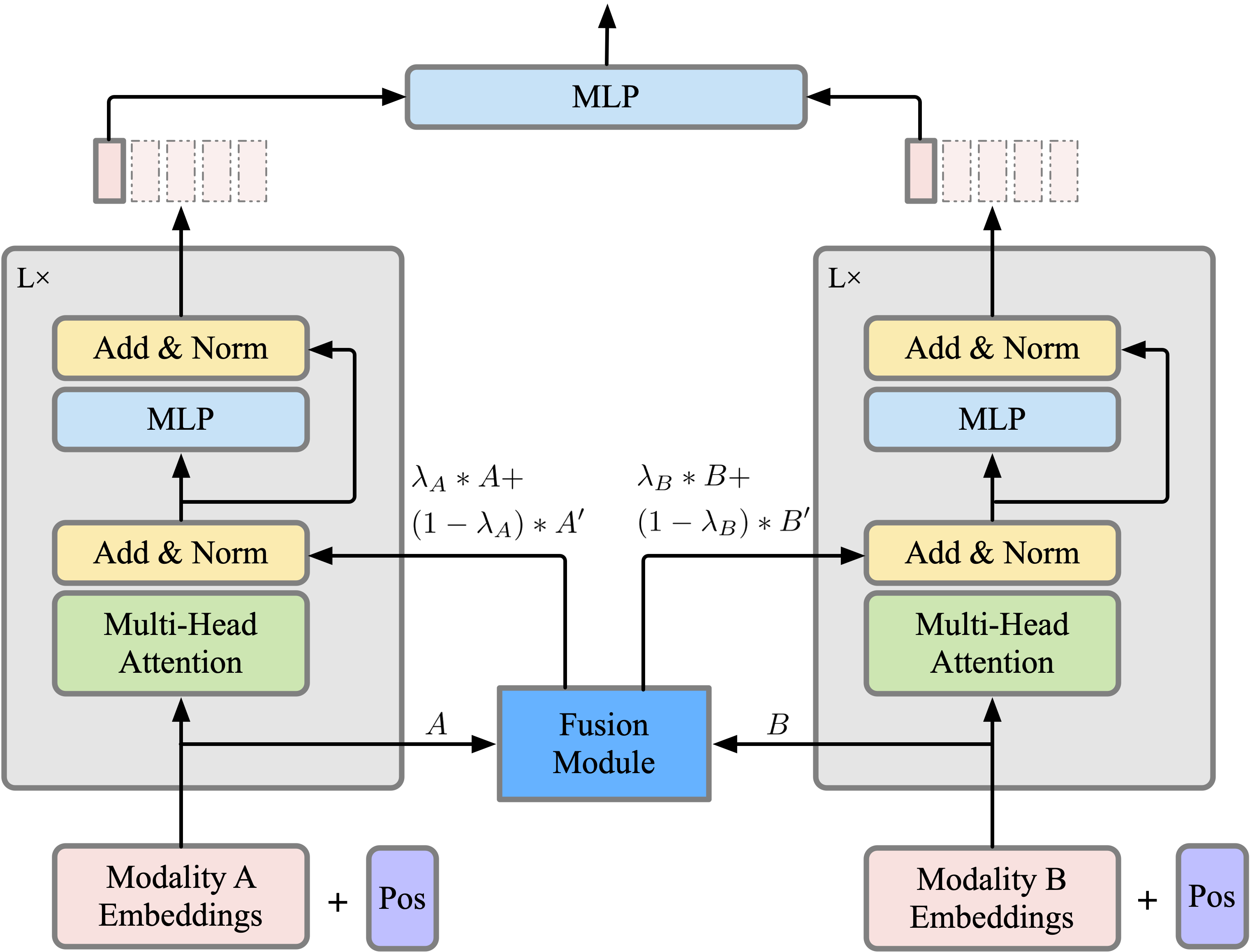
To address point (i), we adopt the transformer Vaswani et al. (2017) architecture, which is capable of handling different modalities. We are aware that using a common architecture for different tasks would potentially degrade the performance. For point (ii), we introduce the Dense Fusion strategy that builds upon the transformer architecture (see Figure 1). The fusion happens at every stage. We also consider one of its variations, which includes weights (’s) to control the fusion intensity. Those weights are learned during the training. Such a variation is referred as the Dynamic Dense Fusion.
To summarize, in our experiments, we consider the Early Fusion, Late Fusion, as well as two variations of the Dense Fusion strategy. All the network models are built upon the transformer architecture. Details can be found in the experiment setup and in the supplementary material.
3.2 The SHAPE Scores
The SHAPE scores are built upon the Shapley value with identifying the set of modalities as players and model accuracy as the utility function. We distinguish two types of SHAPE scores, one captures the marginal contribution of individual modalities, and the other captures the cross-modal cooperation. The SHAPE scores are easy to compute under the general multi-modal learning scenario, no matter how many modalities are involved.
In the following, we use to denote the accuracy of model on the dataset . When discussing the contribution of different modalities, e.g., and , we shall slightly change the symbol to for emphasizing the involved modalities. The set of modalities in is denoted as .
3.2.1 SHAPE Score for Modality’s Marginal Contribution
For the purpose of evaluating the marginal contribution of a modality , we use the scaled Shapley value
| (1) |
where the normalization factor is introduced to align the scores for different models and thus enable cross-model comparison. Similar to the modal-normalization in Gat et al. (2021), we choose to be the model accuracy on the full dataset , i.e., . For simplicity, we will use the abbreviated symbol , when there is no risk of confusion.
As an example, for the two-modal case, we have
where . Extensions to three or more modalities cases are straightforward, and we leave them to the supplementary material.
Baseline Values
The above refers to the absence of modality and should be implemented using some pre-defined baseline values. In the case where only one modality is absent, it is natural to substitute zeros for the missing inputs. However, when both modalities are absent, i.e., , an all-zero input would produce a single deterministic prediction that is sensitive to specific training settings, such as the model initialization. We argue that it is better to predict the majority class in this case. This majority-classifier is stable and could account for the possible unbalances in the dataset.
3.2.2 SHAPE Score for Cross-modal Cooperation
The Shapley value also enables us to directly measure the cross-modal cooperation, which evaluates the degree to which the model exploits the complementary information of a modality provided to the other modalities.
Intuitively, to compute the cooperation among a set of modalities , we need to subtract the marginal contributions of all from the marginal contribution of itself. Treating as a single effective player, its marginal contribution can be evaluated by . On the other hand, the marginal contribution of should be . Consequently, the cooperation score is defined as
| (2) |
Note that the set of ”players” in the above is different from the one in Equation 1. For simplicity, we usually omit the subscripts and write the score as .
For a concrete example, let’s consider the two-modal case. After a few steps of simple algebra, we arrive at
where and denote the baseline values for modalities , respectively.
3.3 Fine-grained Perceptual Scores
In this subsection, we proceed to have a closer look at the perceptual score Gat et al. (2021). First, we will show that this score implicitly measures the correlation among different modalities within the dataset . Then we propose a fine-grained version of the perceptual score. In the following, we only keep the key steps and leave the detailed deduction to the supplementary material.
Let denote a data sample in , where is the input feature and is the corresponding label. In order to explicitly refer the modalities, we will decompose as , where and are the subsets of modalities. Recall that the model accuracy is defined as , where is the identity function and refers to the model prediction at input . Simple algebra will lead us to
where is the probability distribution on .
The permutation-based step in the perceptual score would alter the data distribution, resulting in a new effective dataset with distribution . We refer to this effective dataset as . Now, the perceptual score for is
where . Clearly, apart from the dependence on the model through , the term effectively measure the correlation between and in the dataset .
Since is non-negative, if the part comes from the same class as , then we would expect . We refer to this case as the in-class permutation. Likewise, in the out-class permutation, comes from a different class from and we expect .
The in-class and out-class cases provide conflicting driving forces that would cancel each other and cannot be reflected by the original perceptual score. Based on this observation, we propose to use the in-class and out-class perceptual scores in place of the original one. They are defined as following:
where the operator removes the modality either by the in-class permutation () or the out-class permutation (). is the normalization factor as usual. We only consider the model-normalization here. Finally, for simplicity, we usually omit the subscripts as long as it raises no confusion.
4 Experiments
| B-T4SA | SHAPE scores | (fine-grained) perceptual scores | ||||||||||
|---|---|---|---|---|---|---|---|---|---|---|---|---|
| Acc. | ||||||||||||
| Unimodal V | 41.95 | – | – | – | – | – | – | – | – | – | ||
| Unimodel T | 94.89 | – | – | – | – | – | – | – | – | – | ||
| Early Fusion | 95.01 | |||||||||||
| Late Fusion | 95.22 | |||||||||||
| Dense Fusion | 94.97 | |||||||||||
| Dynamic Fusion | 95.36 | |||||||||||
| CMU-MOSEI | SHAPE scores | (fine-grained) perceptual scores | ||||||||||
|---|---|---|---|---|---|---|---|---|---|---|---|---|
| Acc. | ||||||||||||
| Unimodal A | 71.04 | – | – | – | – | – | – | – | – | – | ||
| Unimodel T | 80.20 | – | – | – | – | – | – | – | – | – | ||
| Early Fusion | 80.22 | -0.01 | 11.46 | -0.02 | ||||||||
| Late Fusion | 80.67 | 0.04 | 11.89 | 0.09 | ||||||||
| Dense Fusion | 79.04 | 0.19 | 9.93 | 0.38 | ||||||||
| Dynamic Fusion | 80.05 | -0.21 | 11.47 | -0.42 | ||||||||
| SNLI | SHAPE scores | (ffine-grained) perceptual scores | ||||||||||
|---|---|---|---|---|---|---|---|---|---|---|---|---|
| Acc. | ||||||||||||
| Unimodal | 33.84 | – | – | – | – | – | – | – | – | – | ||
| Unimodel | 66.32 | – | – | – | – | – | – | – | – | – | ||
| Early Fusion | 82.47 | |||||||||||
| Late Fusion | 69.77 | |||||||||||
| Dense Fusion | 84.91 | |||||||||||
| Dynamic Fusion | 85.02 | |||||||||||
4.1 Setup
For all models, we use 4-layer transformer encoder as the backbone. The number of attention heads is 8, and the hidden dimension is 1024. All models are trained using the Adam optimizer with learning rate warm-up in the first epoch. We encode text data with the GloVe Pennington et al. (2014), and audio data with the MFCC Tiwari (2010). As for the image data, we employ the patch embedding technique, following the ViT Model Dosovitskiy et al. (2020). It is worth noting that our models achieve comparable performance with the supervision-based SOTA models.
4.2 Datasets
Real-life applications raise diverse demands for multi-modal data. Depending on specific tasks, some must be handled by combining all the involved modalities, while in the others, additional modalities merely provide complementary information. Furthermore, different modalities in a multi-modal dataset might be only weakly correlated to each other, or they could be different representations that provide precisely the same information. To account for those complicated situations, we deliberately choose three datasets, as will be introduced below.
B-T4SA
The dataset Vadicamo et al. (2017) is collected from Twitter, including the posted text (textual modality T) and associated images (visual modality V). Each data pair is annotated with a sentiment label (positive, negative and neutral). The task is to predict this label using both the text and image inputs. We note that the text data normally align with their sentiment labels while a large number of images seem to be irrelevant to the labels. B-T4SA represents the situation that different modalities are complementary and weakly correlated to each other.
CMU-MOSEI
This dataset Zadeh et al. (2018) is the largest dataset for sentence-level sentiment analysis and emotion recognition. It contains more than 65 hours of annotated video data, consisting of audio, video and text modalities. In our experiments, we only use the audio (A) and text (T) modalities. The text modality includes the scripts that are generated from the audio data. In this way, the CMU-MOSEI dataset stands for the situation that different modalities are complementary and highly correlated.
SNLI
The SNLI dataset Bowman et al. (2015) is a collection of 570k human-written English sentence pairs. Each pair contains a premise and a hypothesis, whose relation is labeled as either entailment, contradiction, or neutral. We shall view the premise and hypothesis as two distinct modalities, i.e., and . The underlying task is to infer the relationship between the premise and the hypothesis. Clearly, this task intrinsically relies on both modalities and, thus, represents the situation that different modalities are indispensable.
4.3 Contribution and Cooperation
In this subsection, we investigate the SHAPE scores across different models on the three multi-modal datasets, demonstrating their ability in capturing the marginal contribution of individual modalities and the cross-modal cooperation.
Table 1 summarizes the results for B-T4SA dataset. We find the unimodal model for T performs as good as multi-modal models, while the unimodal model for V only slightly suppasses the random guess. The SHAPE scores align with these observations. The contribution scores for V modality are near zero for all the fusion strategies, indicating V almost does not contribute to the task. Further, the cooperation scores are very small as well. Hence, as expected, nearly no cooperation happens between the two modalities. At last, we note that for early fusion and dense fusion are evidently higher than the other two models. This may be attributed to the fact that both the early and the dense fusion models encourage the fusion between the two modalities.
The A modality in the CMU-MOSEI dataset encodes richer information than its text counterparts by including features such as the tone and the talking speed. On the other hand, the T modality is better at representing semantic information. One would expect a multi-modal model to actively integrate the two modalities and make better predictions. Unfortunately, it is not the case as indicated by the SHAPE scores (see Table 2). Values of and are very small, indicating the audio data seldom contribute to the model performance and there is little cooperation between the A and T modalities. In addition, the marginal contributions of T modality, , are also relatively small. At first sight, it may seem contradictory that both modalities have limited contribution to the performance, while the model achieves a decent accuracy. Closer investigation reveals that this is a consequence of the unbalanced dataset. Simply by predicting positive, one could get an accuracy of , which is the accuracy of the unimodal model for A. This phenomenon coincides with the common belief that the deep neural networks are lazy, tending to take shortcuts. It could be the case that the multi-modal models simply exploit the unbalance of the dataset and pay little effort in mining the cooperation.
In Table 3, we show the results for the natural language inference task on the SNLI dataset, for which both modalities are indispensable. We find that both unimodal models perform poorly. Interestingly, the unimodal model for significantly outperforms the random guess. This implies that there could be implicit biases within the dataset despite that it is balanced. As expected, the behavior of SHAPE scores is different from previous cases. and becomes comparable, with being generally higher. Hence, both modalities contribute, and the hypothesis is more important for model prediction. More strikingly, the cooperation scores are also high. This suggests that the models actively exploit the cooperation between and for predictions. At last, in the late fusion case, and are much lower than the other cases. The lack of cooperation could be attributed to the nature of the late fusion strategy, i.e., the fusion only happen at the last step. This helps explain the low accuracy of the late fusion model and suggest that, in this case, fusion at earlier stages is a better choice.
4.4 Compared with the Perceptual Score
In this subsection, we compare our SHAPE scores with the perceptual score as well as with its fine-grained versions.
Firstly, we observe that the perceptual score coincides with our marginal contribution SHAPE score in the sense that their values are highly correlated. In the B-T4SA dataset, both and are close to zero, and () is significantly higher than (). Similar pattern is found in the CMU-MOSEI dataset. For the SNLI dataset, and are both considerably higher than zero, except for the Late Fusion case. Besides, both scores for modality are higher than the ones for modality.
Despite the similarities, we emphasize the superiority of our SHAPE scores for (i) guaranteed by the game theory, the SHAPE score can correctly capture the marginal contribution no matter how many modalities are involved. (ii) the SHAPE score can directly quantify the cooperation among modalities in addition to their individual importance.
Next, we turn to the fine-grained perceptual scores. As argued in section 3.3, the raw perceptual score implicitly measures the correlation among modalities in the dataset. However, the positive and negative correlations are mixed and cancel each other, causing a considerable loss of information. To be concrete, let’s consider the Late Fusion case for the SNLI dataset. With only the raw perceptual scores, we at best might conclude that the modality is more important than the one in the contribution to model performance. On the other hand, we find is much smaller than , indicating that the model prediction almost relies solely on the modality. The small values of and further consolidate this conclusion. Putting it differently, the Late Fusion model tends to use only the modality while ignoring the modality. Consequently, the cooperation between the two modalities should be small in the Late Fusion case. This is just what the cooperation SHAPE score reveals to us. Under more complicated scenario with three or more modalities, it would be harder to capture the cross-modal cooperation using perceptual scores. On the contrary, it is always straightforward to quantify the cross-modal cooperation with the SHAPE score .
5 Discussion
The above experiment results suggest that the way a model exploits multi-modal information depends on various factors, including the intrinsic correlation among individual modalities in the dataset, the type of the task, and the fusion strategy in use. Based on this observation, we want to draw attention to dataset and task in multi-modal learning research. There is little hope to train a model that can exploit cross-modal cooperation on a dataset where different modalities are nearly independent. Likewise, if the task can be easily handled with only a single modality, one must try hard to design an algorithm to exploit the possible cross-modal cooperation. Furthermore, the bias and unbalance in dataset also affect multi-modal learning. In many cases, the improvement in the accuracy of a multi-modal model could be illusive. Our SHAPE score can directly quantify the cooperation among individual modalities and, hence, could help diagnose the fusion strategy.
At last, it is worth noting that though the present SHAPE scores are defined using the accuracy metric as the utility function, there is no limitation of what function should be used. In fact, the SHAPE scores can readily adapt to more complex metrics such as the F1 score.
6 Conclusion
In this paper, we present the SHAPE scores that quantify the marginal contribution of individual modalities and their collaboration. Properties of the Shapely value provides theoretical guarantee for the validity of our SHAPE scores and the experiments empirically verify their effectiveness. We would like to suggest using the SHAPE scores in addition to the accuracy metric when analyzing a multi-modal model, as they are easy to compute and can extract key information about how the model use multi-modal data.
We are aware that the present SHAPE scores are not yet perfect. The choice of baseline values deserve more deliberate consideration. In the future work, we will keep improving the SHAPE scores and systematically evaluate the SOTA multi-modal models.
Acknowledgments
This work was supported by grants from the National Science and Technology Innovation 2030 Project of China to Yi Zhou (2021ZD0202600).
References
- Antol et al. (2015) Antol, S., Agrawal, A., Lu, J., Mitchell, M., Batra, D., Zitnick, C. L., and Parikh, D. Vqa: Visual question answering. In Proceedings of the IEEE international conference on computer vision, pp. 2425–2433, 2015.
- Bai et al. (2021) Bai, C., Chen, H., Kumar, S., Leskovec, J., and Subrahmanian, V. S. M2P2: Multimodal Persuasion Prediction using Adaptive Fusion. arXiv preprint arXiv:2006.11405, December 2021. URL http://arxiv.org/abs/2006.11405.
- Baltrušaitis et al. (2018) Baltrušaitis, T., Ahuja, C., and Morency, L.-P. Multimodal machine learning: A survey and taxonomy. IEEE transactions on pattern analysis and machine intelligence, 41(2):423–443, 2018.
- Bowman et al. (2015) Bowman, S. R., Angeli, G., Potts, C., and Manning, C. D. A large annotated corpus for learning natural language inference. arXiv preprint arXiv:1508.05326, 2015.
- Delbrouck et al. (2020) Delbrouck, J.-B., Tits, N., Brousmiche, M., and Dupont, S. A transformer-based joint-encoding for emotion recognition and sentiment analysis. arXiv preprint arXiv:2006.15955, 2020.
- Dosovitskiy et al. (2020) Dosovitskiy, A., Beyer, L., Kolesnikov, A., Weissenborn, D., Zhai, X., Unterthiner, T., Dehghani, M., Minderer, M., Heigold, G., Gelly, S., et al. An image is worth 16x16 words: Transformers for image recognition at scale. arXiv preprint arXiv:2010.11929, 2020.
- Gat et al. (2021) Gat, I., Schwartz, I., and Schwing, A. Perceptual score: What data modalities does your model perceive? Advances in Neural Information Processing Systems, 34, 2021.
- Goyal et al. (2017) Goyal, Y., Khot, T., Summers-Stay, D., Batra, D., and Parikh, D. Making the v in vqa matter: Elevating the role of image understanding in visual question answering. In Proceedings of the IEEE Conference on Computer Vision and Pattern Recognition, pp. 6904–6913, 2017.
- Hessel & Lee (2020) Hessel, J. and Lee, L. Does my multimodal model learn cross-modal interactions? it’s harder to tell than you might think! arXiv preprint arXiv:2010.06572, 2020.
- Kiela et al. (2019) Kiela, D., Bhooshan, S., Firooz, H., Perez, E., and Testuggine, D. Supervised multimodal bitransformers for classifying images and text. arXiv preprint arXiv:1909.02950, 2019.
- Liang et al. (2021) Liang, P. P., Lyu, Y., Fan, X., Wu, Z., Cheng, Y., Wu, J., Chen, L., Wu, P., Lee, M. A., Zhu, Y., Salakhutdinov, R., and Morency, L.-P. MultiBench: Multiscale Benchmarks for Multimodal Representation Learning. arXiv preprint arXiv:2107.07502, November 2021. URL http://arxiv.org/abs/2107.07502.
- Liu et al. (2019) Liu, F., Liu, J., Fang, Z., Hong, R., and Lu, H. Densely connected attention flow for visual question answering. In IJCAI, pp. 869–875, 2019.
- Lundberg & Lee (2017) Lundberg, S. M. and Lee, S.-I. A unified approach to interpreting model predictions. In Proceedings of the 31st international conference on neural information processing systems, pp. 4768–4777, 2017.
- Molnar (2020) Molnar, C. Interpretable machine learning. Lulu. com, 2020.
- Pennington et al. (2014) Pennington, J., Socher, R., and Manning, C. D. Glove: Global vectors for word representation. In Proceedings of the 2014 conference on empirical methods in natural language processing (EMNLP), pp. 1532–1543, 2014.
- Rodrigues Makiuchi et al. (2019) Rodrigues Makiuchi, M., Warnita, T., Uto, K., and Shinoda, K. Multimodal fusion of bert-cnn and gated cnn representations for depression detection. In Proceedings of the 9th International on Audio/Visual Emotion Challenge and Workshop, pp. 55–63, 2019.
- Shapley (1953) Shapley, L. The value of n-person games. Annals of Math. Studies, 28:307–317, 1953.
- Tiwari (2010) Tiwari, V. Mfcc and its applications in speaker recognition. International journal on emerging technologies, 1(1):19–22, 2010.
- Vadicamo et al. (2017) Vadicamo, L., Carrara, F., Cimino, A., Cresci, S., Dell’Orletta, F., Falchi, F., and Tesconi, M. Cross-media learning for image sentiment analysis in the wild. In Proceedings of the IEEE International Conference on Computer Vision Workshops, pp. 308–317, 2017.
- Vaswani et al. (2017) Vaswani, A., Shazeer, N., Parmar, N., Uszkoreit, J., Jones, L., Gomez, A. N., Kaiser, Ł., and Polosukhin, I. Attention is all you need. In Advances in neural information processing systems, pp. 5998–6008, 2017.
- Wang et al. (2020) Wang, W., Tran, D., and Feiszli, M. What Makes Training Multi-Modal Classification Networks Hard? arXiv preprint arXiv:1905.12681, April 2020. URL http://arxiv.org/abs/1905.12681.
- Wang (2021) Wang, Y. Survey on deep multi-modal data analytics: collaboration, rivalry, and fusion. ACM Transactions on Multimedia Computing, Communications, and Applications (TOMM), 17(1s):1–25, 2021.
- Weber (1988) Weber, R. J. Probabilistic values for games. The Shapley Value. Essays in Honor of Lloyd S. Shapley, pp. 101–119, 1988.
- Zadeh et al. (2018) Zadeh, A. B., Liang, P. P., Poria, S., Cambria, E., and Morency, L.-P. Multimodal language analysis in the wild: Cmu-mosei dataset and interpretable dynamic fusion graph. In Proceedings of the 56th Annual Meeting of the Association for Computational Linguistics (Volume 1: Long Papers), pp. 2236–2246, 2018.
Appendix A Appendix
A.1 Model Details
Setting
Here we define the A,B as the input embedding of two modalities. Moreover, all models use a four-layer transformer encoder module as the backbone, including both the unimodal model and multi-modal modal. The encoder module can be described as follows:
-
•
Component 1. A Multi-Head Self-attention module with a residual operation:
-
•
Component 2. A Feedforward module with a residual operation , where FFNN function is calculated by
-
•
Component 3. A MLP module that consists of only a one-layer Linear module, which projects the dimension of the hidden layer to the dimension of class numbers.
In addition, we add a learnable token to the sequence of embedded features ( The function is similar to the BERT [class] token ), and a position embedding is added to the embedded features.
A.1.1 Early Fusion Model
In the Early fusion model, we simply implement the operation on each modality’s embedding feature: . Then we combined embedding as the input to a one pathway transformer encoder-based model.
A.1.2 Late Fusion Model
In the Late fusion model, we first use two pathway structures to learn the representations of individual modalities independently, and then we combine the first vector of the last output hidden layer from each pathway to be the final output. The model’s architecture is the same as Figure 1 but does not have the fusion model.
A.1.3 Dense Fusion Model
In the dense fusion model, we integrate modalities using a Multi-head Self-attention module to learn co-representation between two modalities. The operation consists of two steps:
-
1.
We get the co-representation and by .
-
2.
We make modalities fusion operation by and which allows the model to fuse the co-representation with individual modalities representation. We implement this operation on every layer of the transformer encoder model.
A.1.4 Dynamic Dense Fusion Model
The architecture of this model is similar to the Dense Fusion Model, but we add a learned parameter to dynamic control how much the co-representation can be integrated into each modalities’ pathway. The process can be described as follows:
-
1.
We get the co-representation and by .
-
2.
We get the parameter by a Gate Function which can be wrote by pytorch-like code as follows:
where the is the number of that needs to be learned in our multi-modal models, which also means the number of the modalities used in our model. We make modalities fusion operation by and .
Appendix B Deduction Detail
B.1 Example of the SHARP Score for Three-modality Case
Here we provide an concrete example of the marginal contribution in the three-modality case, i.e.,
B.2 Perceptual Score
The model accuracy is defined as
where is model prediction and refers to the set of possible labels.
We proceed as follows:
where is the predicted label at , and in the last step we use following equation,
The permutation step in the perceptual score will alter the data distribution and results in a new effective dataset . Suppose we are calculating the perceptual score for modality set , the discribution of will be . Through similar steps, we arrive at
Then, the perceptual score can be expressed as