Baselines and Protocols for Household Speaker Recognition

Abstract

Speaker recognition on household devices, such as smart speakers, features several challenges: (i) robustness across a vast number of heterogeneous domains (households), (ii) short utterances, (iii) possibly absent speaker labels of the enrollment data (passive enrollment), and (iv) presence of unknown persons (guests). While many commercial products exist, there is less published research and no publicly-available evaluation protocols or open-source baselines. Our work serves to bridge this gap by providing an accessible evaluation benchmark derived from public resources (VoxCeleb and ASVspoof 2019 data) along with a preliminary pool of open-source baselines. This includes four algorithms for active enrollment (speaker labels available) and one algorithm for passive enrollment.

1 Introduction

Speech technology has entered our living rooms. Be it a smart TV or smart home assistant connected to other devices, an increasing number of commercial products now support interaction by voice. In addition to recognizing voice commands correctly (speech recognition), it is important to be aware of the user (speaker identification) for customized experiences such as personalized playlists, recommendations and bookings.

We address such household speaker recognition task [1, 2] where a small group of users (household members) share a common device. The task is differentiated from generic speaker recognition tasks (addressed in standard benchmark data such as NIST SREs [3] and VoxCeleb [4, 5]) with several desiderata, intended to maximize user experience:

• Domain robustness. The device should be readily-usable in previously unseen domains (households);

• User convenience. User registration (speaker enrollment) should be done as unobtrusively as possible --- ideally without any interaction with the user;

• Adaptivity. To maintain high performance through weeks, months, or years, the model(s) require updating (again without user interaction);

• Short utterances. The device should be attentive to the user with very short utterances (1-2 second range);

• Open-set operation. The device should be attentive only to the members of a given household, i.e. the ability to ignore commands from unknown (out of the household) users;

• Computational efficiency. With growing privacy concerns, it might be preferable to carry out on-device computations without sending the user’s speech data elsewhere.

The above translate to computationally light and ideally unsupervised (no speaker labels required) approaches that evolve with time, as opposed to single-shot optimization on a given corpus, domain, or challenge.

In generic speaker recognition setups, the issue of speech variation across different datasets is typically addressed using domain adaptation (DA) of an already well-trained recognizer. Practice has shown that it is effective to first train a large speaker embedding network (that serves as a utterance-level speaker feature extractor) [6, 7], fix it across domains, followed by adaptation of back-end classifier (speaker comparator) to each domain of interest [8, 9, 10, 11].

While DA methods are designed to address small number of large domains (many speakers), the household scenario represents the opposite --- large number of small domains (households). As noted in [2], systems designed to address generic speaker recognition task on large population might be suboptimal on specific speaker subsets with homogeneous data. Homogeneous data can indeed be expected due to the shared device with the fixed (or infrequently changed) location. The household scenario is therefore differentiated from speaker recognition across devices or on mobile devices. In addition, DA methods are typically not designed to handle sequential (online) data arriving one utterance at a time. For these reasons, we consider lightweight back-ends with as few parameters as possible and instead focus on adapting speaker-specific representations (here, deep neural embeddings).

Speaker recognition for household scenarios is a relatively recent direction (at least in the published literature) [1, 2]. In [1], enrichment of speaker-specific representation using unlabeled data is achieved through semi-supervised label propagation [12]. Another study [2] considers a neural back-end classifier with lower-dimensional space, into which the extracted embeddings are mapped. This space is optimized for a given speaker subset. Even if we draw inspiration from these prior studies, there is an important difference in the assumptions. Specifically, we argue that in households one must prepare for the possibility of external non-target speakers, or guests. Therefore, the label propagation approach in [1] is not directly applicable for potential unknown (out of household) speakers.

We summarize our contributions as follows. First and foremost, given the sparse literature and lacking common methodological standards, we target our study to researchers and practitioners who look for an accessible and reproducible starting point to address household speaker recognition tasks. The methodology sections, therefore, provide a guided taxonomy of methods and suggested terminologies. Importantly, we make our experimental pipeline, methods, and protocols public both for reproducibility and for promotion of further research on this topic.

Besides advancing evaluation infrastructure as described above, we have a number of algorithmic and experimental design-related contributions too. In terms of algorithms, we modified several existing clustering algorithms including the one from [13] by introducing an extra ‘‘background class’’ and allowing for partially labeled data. Second, we consider a highly-constrained variant of probabilistic linear discriminant analysis (PLDA) back-end [14, 15] involving spherical covariances. This results in an equivalent scoring rule with the widely-used cosine similarity in the case of a single enrollment utterance, with an added benefit of improved score calibration for multiple enrollment utterances.

In terms of experimental design, while we draw inspiration from [1, 2], we suggest a number of extensions and improvements to the simulation of household speaker recognition tasks. Similar to [1, 2] we use the public VoxCeleb data [4, 5] in our experiments. In addition, we leverage another public dataset, ASVspoof 2019 physical access (PA) task [16]. Even if the primary use of this dataset is that of benchmarking spoofing countermeasures, in this work we focus on bonafide scenarios (no spoofing attacks). The ASVspoof 2019 PA data consists of carefully controlled simulated environments with variations in room sizes, reverberation time, and talker-to-microphone distances. As opposed to VoxCeleb (crawled from YouTube) where randomly-paired utterances may not be representative of a shared homogenous environment, the ASVspoof 2019 PA data allows a design aligned closer with the assumptions of household scenarios; speakers for a given household are selected from the same simulated environment. The experiments with both simulated environments (ASVspoof 2019) along with ‘in the wild’ style data (VoxCeleb) used in prior studies, therefore, complement one another.

2 Household Speaker Recognition

2.1 General task set-up and data assumptions

Before presenting the methodology details, we set the general stage for the household speaker recognition task. A household is a small set of natural persons (such as family members) whose voice data is processed by a shared device. The task of interest is open-set speaker identification (SID) [17] that aims at classifying an unseen utterance $X$ either as one of the $N$ known household members, or an additional $(N+1)$:th ‘none of the known speakers’ class. We refer to such speakers as guests.

At the enrollment (registration) stage, the device collects voice data of the household members to create the speaker-specific model(s). In generic speaker recognition tasks, the speaker labels of enrollment data are typically available and trustworthy. For instance, published corpora and challenge datasets may undergo tedious scrutiny to validate the correctness of speaker labels (and other metadata) before their release. With similar quality control in mind, in the household scenario, the user might be prompted to repeat wake words or read other pre-specified text passages to create a personal profile. As such active enrollment could be time-consuming or otherwise inconvenient, a more attractive alternative is to collect speech data while the device is used and use speaker clustering to infer pseudo speaker labels after a sufficient amount of data has been collected. The user might then be asked for consent for profile creation. Following terminology used in some commercial products, we refer to such procedures as passive enrollment. In this work, we consider both active and passive enrollment strategies.

Besides the test and enrollment data, we assume an additional set of unlabeled adaptation data to be available for updating speaker-specific models. Such unsupervised speaker adaptation was introduced to the NIST speaker recognition evaluation (SRE) series in 2004 [3]. This task is not to be confused with techniques such as transfer learning [18, 19] or domain adaptation [8, 9, 10, 11] that re-train or modify selected parameters of the recognizer itself. In this work, both the speaker embedding extractor and classifier remain fixed whereas speaker-specific models undergo frequent updates.

Since adaptation data is unlabeled, the decision as to which speaker model (if any) should be updated has to be done by the recognizer automatically. Note that an error-free (oracle) SID system leads to an effectively larger amount of enrollment data per user. In any practical case, however, the SID system makes errors, leading to potentially updating incorrect speaker model(s).

One of the differences between the household speaker recognition from generic speaker recognition evaluation setups is the varying amount of data available for speaker enrollment and model updating. In contrast to, e.g., VoxSRC challenge setup with a single enrollment utterance per trial [20], in the household scenario we assume that multiple utterances can be used to construct the speaker model. Further, the number of utterances may vary from speaker to speaker. This corresponds to multi-enrollment speaker verification [21, 22].

2.2 General procedure

Moving on from the data requirements towards methodology, the core task of interest is pairwise comparison of test utterance with hypothesized model(s). In this study, we use different deep neural embeddings [23] to represent speech utterances. In particular, utterance $X$ of arbitrary duration is represented using a speaker embedding $\boldsymbol{x}\in\mathbb{R}^{d}$ of $d$ dimensions: $\boldsymbol{x}=\texttt{dnn}(X)$. Here $\texttt{dnn}(\cdot)$ is either E-TDNN [7], ECAPA-TDNN [6] or a Resnet34 (details in Section 6.2) used for processing both enrollment and test data. We consider these embedding extractors fixed and focus on the system back-end.

The underlying computational task is that of creating a speaker representation (speaker model) for each household member using enrollment and speaker adaptation data. We consider two types of speaker representations, based on sets and centroids. In the former, a speaker is represented by a collection of embeddings extracted from the utterances of that speaker. In the latter, in turn, we maintain only a single averaged embedding (centroid) per speaker. One can always switch from the set representations to centroids, but not in the other direction. We used one of these representations depending on the speaker adaptation algorithm.

In terms of adaptation algorithms, we consider several alternatives categorized either as online (sequential) or offline (batch) methods. Whereas the former (Section 4) assumes the unlabeled adaptation data to arrive utterance-by-utterance, the latter (Section 5) assumes the adaptation data of all speakers to be available at once. While the former might be preferable from a computational point of view, the latter has the potential to benefit from the global structure of adaptation data. A common ingredient to all considered adaptation algorithms is scoring function (Section 3) that produces a speaker similarity score between $\boldsymbol{x}$ and hypothesized speaker model(s).

Algorithm 1 Active enrollment with online updates

• Labeled enrollment data $\mathcal{X}_{\text{enroll}}=\{(\boldsymbol{x}_{i},y_{i})\}$ from one household with speakers $y_{i}\in\{1,2,\dots,K\}$.

• Unlabeled adaptation data $\mathcal{X}_{\text{a}}=\{\boldsymbol{x}_{t}\}$ containing both household members and guests.

One model $\boldsymbol{\theta}_{y}$ per speaker $y\in\{1,2,\dots,K\}$.

for $y\in\{1,2,\dots,K\}$ do $\triangleright$ Enroll each speaker

     $\boldsymbol{\theta}_{y}\leftarrow$ ENROLL$\Big{(}\{\boldsymbol{x}_{i}\in\mathcal{X}_{\text{e}}:y_{i}=y\}\Big{)}$

end for

for $\boldsymbol{x}\in\mathcal{X}_{\text{a}}$ do $\triangleright$ Online model update

     $k^{*}\leftarrow\arg\max_{k}\texttt{SCORE}(\boldsymbol{x},\boldsymbol{\theta}_{k})$

     if $\texttt{SCORE}(\boldsymbol{x},\boldsymbol{\theta}_{k^{*}})>\tau$ then

         $\boldsymbol{\theta}_{k^{*}}\leftarrow\texttt{UPDATE}(\boldsymbol{x},\boldsymbol{\theta}_{k^{*}})$

     end if

end for

Algorithm 1 outlines a generic template for active enrollment with online updates: after active speaker enrollment, data arrive one by one. The top-scoring model is updated if the speaker similarity score exceeds an update threshold, and none of the other models are updated.

Note that the presented generic algorithm assumes discarding presumably out-of-set embeddings without any further processing. However, in principle, these embeddings could be utilized for representing the impostor class corresponding to all the possible guest speakers.

Algorithm 2 Passive enrollment

• Unlabeled adaptation data $\mathcal{X}_{\text{a}}=\{\boldsymbol{x}_{t}\}$ containing both household members and guests.

$\boldsymbol{\theta}=\{\boldsymbol{\theta}_{1},...,\boldsymbol{\theta}_{K}\},K\leftarrow\texttt{CLUSTER}(\{\boldsymbol{x}_{t}\in\mathcal{X}_{\text{a}}\}$)

$\triangleright$ Perform clustering

In the passive enrollment scenario, one needs to evaluate the ability of the speaker recognition system to identify clusters corresponding to speakers in an unlabeled adaptation set as shown in Algorithm 2. Evaluating the success of passive enrollment is therefore similar to the evaluation of general clustering algorithms: given a set of data points, the performance of a clustering algorithm is measured by comparing the predicted groups to the ground-truth partition. There are some minor differences, however. In particular, not all clusters are equally important. Specifically, we assume that there are several dominating clusters in the set, representing the classes of interest. These target clusters represent household members. The aim is to correctly identify only these clusters, while the predicted partitions for the rest of the data set can be arbitrary. In other words, if a pair of guest speakers were incorrectly grouped into a single cluster, it should not affect the performance metric.

3 Scoring Back-Ends

In this section, we discuss considerations related to the choice of speaker representation and scoring back-ends. Recent challenges including VoxSRC [20, 24] and VOiCES 2019 [25] indicate cosine scoring to be a common choice with speaker embedding extractor networks trained with variants of angular margin softmax losses such as AM-Softmax and AAM-Softmax [26, 27]. Another popular choice is PLDA which is more efficient in combination with x-vector embeddings [28, 29].

As for the latter, we consider PLDA model with the full-rank speaker subspace, in the form of a two-covariance model [14]. It is specified by two covariance matrices, representing between- and within-speaker covariances. We choose to use spherical covariances (scaled identity matrices). Despite being a highly constrained full-covariance PLDA, this low-parameter version may have an edge in the household speaker recognition scenario. In particular, a model with only two scalar parameters can be presumed to be more robust against domain mismatch compared to full-covariance PLDA which usually requires domain adaptation to the target domain [30, 9]. In our experiments, we use embedding averaging for all models apart from this spherical covariance PLDA that uses the so-called by-the-book scoring [21] for multiple enrollment utterances.

It can be shown that the spherical covariance PLDA is equivalent to cosine scoring in the case of a single enrollment utterance. See Appendix 10.1 for the detailed derivation.

4 Online Algorithms

We now detail the algorithm that processes data sequentially, in an online manner. In what we refer to as centroid model with exponential smoothing, each of the $K$ speakers in a given household is represented by a centroid (average vector) of enrollment data. Call these (initial) centroids $\{\boldsymbol{c}_{k}^{(0)}\},k=1,\dots,K$. At each time-step $t=1,2,\dots$ we obtain a new utterance represented by speaker embedding $\boldsymbol{x}^{(t)}$, which is compared with all the centroids to obtain $K$ similarity scores $s_{1}^{(t)},\dots,s_{K}^{(t)}$. Here these scores are computed either using cosine similarity or PLDA [14].

Let $k^{(t)}_{*}\equiv\arg\max_{1\leq k\leq K}\{s_{k}^{(t)}\}$ denote the highest scoring speaker and $s^{(t)}_{*}$ the corresponding score. We update the centroid of the previous time step if and only if $s^{(t)}_{*}>\tau$, by

$$\boldsymbol{c}_{k^{*}}^{(t)}=\alpha\boldsymbol{x}^{(t)}+(1-\alpha)\boldsymbol{c}_{k^{*}}^{(t-1)},$$ (1)

where $\tau$ and $\alpha$ are control parameters. Update concerns only the top-scoring centroid and no update takes place if $s^{(t)}_{*}\leq\tau$.

The update rule (1) corresponds to exponential smoothing [31] where the updated centroid is a weighted average of the current embedding and the current centroid. Thus, $0\leq\alpha\leq 1$ serves as smoothing factor that controls the rate at which the centroids evolve. Larger values of $\alpha$ correspond to a stronger emphasis on the most recent observation. Note that simple averaging of embeddings fits this update rule too if one relaxes the assumption of the smoothing factor to be a constant and sets it instead as $\alpha_{t}=1/(t+1)$. In summary, the method has two control parameters $\alpha$ and $\tau$. We address their role in the experimental part. For practical purposes, they are tuned with the aid of a development set.

One can see that the update rule (1) does not track the number of performed updates. However, the information about the number of averaged embeddings is required for the PLDA by-the-book scoring. At the same time, the number of updates may not be an adequate measure of the accumulated information since it depends on the value of the smoothing factor (e.g. consider $\alpha\approx 1$). We address this issue by proposing a heuristic rule to define the zero-order statistics (counts) in the case of weighted averaging of embeddings. See Appendix 10.2 for the detailed discussion.

5 Offline Algorithms

We now turn attention to offline algorithms that operate under the assumption that the whole adaptation set is available at once. Recall that in the active enrollment scenario a small labeled enrollment set is augmented by an unlabeled adaptation set. This naturally fits the formulation of semi-supervised clustering [32], where additional knowledge about the true labels of a subset of data points is assumed. This observation led us to extend two clustering algorithms to their semi-supervised versions, detailed in the next two subsections.

5.1 Semi-supervised k-means clustering

We propose straightforward modifications to the widely known k-means algorithm [33] for the household adaptation setup. First, we modified the traditional (unsupervised) k-means algorithm to fix the cluster assignments for a subset of embeddings with known speaker labels. Second, we introduced as additional ‘‘background class’’ to allow data points with no cluster assignments, further referred to as outliers. These data points correspond to the guest speakers. Specifically, similar to the centroid model described above, we use a pre-defined threshold $\tau$ to determine whether a given data point should be assigned to the closest cluster or labeled as an outlier (a guest). This restricts the clusters to have a bounded diameter. Here, the threshold is a control parameter which should estimated from data.

Similar to the centroid model, the cluster centers (centroids) are initialized by computing speaker-specific average embeddings from the enrollment data.

5.2 Semi-supervised variational Bayesian clustering

Our second proposed offline algorithm can be viewed as variational Bayesian inference [34] applied to a Gaussian mixture model [35]. In fact, it is a slightly modified version of the clustering algorithm described in [13]. in which the speaker embeddings are assumed to have been generated by the two-covariance PLDA model [14] discussed in Section 3. That is, speakers are modeled by Gaussians with shared covariance but speaker-specific means. By assuming that $K$ speakers are present in a given collection of embeddings, this results in a mixture of $K$ Gaussian components. More details are given in the Appendix 10.3.

We modified the mixture model described in [13] where each component corresponds to a speaker. In particular, we add an extra label to present ‘background class’. In practice, we add one $(K+1)$th component to the mixture model to represent the marginal distribution of embeddings. This component is assumed to model all of the unknown (guest) speakers in the household scenario. Also, similar to the semi-supervised k-means clustering described above, we fixed the component assignments for a subset of embeddings with known speaker labels.

This model requires specifying the prior probabilities corresponding to the mixture components $\boldsymbol{\pi}=\{\pi_{1},\dots,\pi_{K+1}\}$. To define the prior probability for the ‘background class’, we apply a threshold $\tau$ as in the other algorithms. In detail, we define this probability as $\pi_{K+1}=\sigma(\tau)$, where $\sigma(\cdot)$ denotes the sigmoid function. Accordingly, the remaining probabilities $\pi_{k}$ are initialized such that $\sum_{k}\pi_{k}=1$ for $k=1,\dots,K+1$.

5.3 Label propagation

Inspired by recent related work [1], we also consider a label propagation approach [36]. Since the original algorithm is not directly applicable to our open-set scenario with potentially unknown speakers, we introduced an additional pre-filtering step. First, all the embeddings that are not sufficiently close to the initial speaker models are labeled as outliers and removed. This outlier filtering is again controlled by a pre-defined threshold $\tau$. After filtering, we assume the remaining set to consist of household members only. Thus, the conventional label propagation algorithm is applied to this set.

6 Experimental Setup

6.1 Household speaker recognition protocols

We have chosen two public datasets for our experiments: ASVspoof 2019 and VoxCeleb. By drawing inspiration from prior studies [1, 2], we design new evaluation protocols for the household speaker recognition task.

ASVspoof 2019: We consider the bonafide audio data of the physical access (PA) subset of ASVspoof 2019 representing different room conditions [16]. The dataset consists of 27 different room conditions with various room sizes, reverberation times, and talker-to-mic distances. In our experiments, we use the evaluation set consisting of 48 speakers (21 male and 27 female). We set the household sizes as 4, 6, 8, and 10, where each household consists of an equal number of male and female speakers. We create the enrollment list, adaptation list, and trial list considering audio files from the same room condition. The speakers are randomly selected. We also have the same number of guest speakers corresponding to a room but chosen randomly from the remaining speakers. We use three utterances for speaker enrollment, whereas the remaining utterances are used for adaptation. We additionally consider the audio data from the guest speakers for adaptation. The adaptation list contains utterances from the household and guest speakers in a random order. The trial lists consist of only same-gender trials as cross-gender non-target trials are relatively easier than the other.

VoxCeleb: We consider VoxCeleb1 data consisting of 1251 speakers, where audio data was originally collected from YouTube videos [4]. Following the work reported in [2], we have chosen four utterances for enrollment, 10 for evaluation, and 13 for adaptation. Each of the utterances was taken from different videos and we have considered speakers with at least 27 video recordings. Similar to ASVspoof 2019 PA, we have gender-balanced households. The households with sizes 4, 6, 8, and 10 were randomly sampled to create 400 simulated households. Each household has the same number of guests as the number of household members. Similar to ASVspoof 2019, there are no cross-gender trials. We have created two sets of ASV protocols from VoxCeleb1 with disjoint set of speakers. One of them is used as development set whereas the other set is used as test set.

Dataset	Target	Non-target (Known/Unknown)
VoxCeleb-dev	27874	80126 / 108000
VoxCeleb-eval	27706	80294 / 108000
ASVspoof 2019	75600	216000 / 291600

Table 1: Trial statistics of the datasets used for our experiments. (Known/Unknown refers to the non-target trials from the same household speakers/guests.)

To sum up, we designed three different protocols VoxCeleb-dev, VoxCeleb-eval, ASVspoof with trial statistics summarized in Table 1. The VoxCeleb-dev protocol serves as the development set and the remaining two are used for final evaluation.

6.2 Speaker embedding extractors and back-end scoring

X-vector. This speaker embedding extractor is based on Extended TDNN (E-TDNN) [7] x-vector. It is trained on dev set of VoxCeleb2 [5], with 5994 speakers. It acquires 80-dimensional mel filterbank outputs as acoustic features. Having the same architecture from [7], we introduce two modifications: 1) We replace statistics pooling with attentive statistics pooling [37]; 2) For loss function, we substitute the conventional cross-entropy one with additive angular margin softmax [38].

SpeechBrain. This pre-trained model is recently proposed by SpeechBrain [39] with pre-trained model available, based on ECAPA-TDNN [6], another x-vector variant with a hybrid of convolutional and residual building blocks at layers before the pooling layer. It also imports the aforementioned two modifications and the same acoustic features. The pre-trained model is trained on train set of VoxCeleb1 [4] and dev set of VoxCeleb2, which results in 7205 speakers. Both speaker embedding extractors reached promising performance in our pilot experiments .

CLOVA. This pre-trained model is proposed by and described in [40]. It is based on ResNet34 architecture [41] and trained on dev set of VoxCeleb2 [5], with 5994 speakers. The input acoustic feature for training this model is 64-dimensional mel filterbank, with online data augmentation [40]. This pre-trained model is provided by CLOVA . Pilot experiments confirm the promising performance of this model.

Moreover, when extracting the speaker embeddings, before feeding the input audio into the pre-trained models, we perform trimming with a threshold of -20 dB, followed by random chunking with a length of 2 seconds, elaborating the short-duration property of the audios under the household scenario.

We used different scoring back-ends depending on the type of embedding. For the x-vector embeddings, we used the conventional back-end including linear discriminant analysis, length normalization, and the full-rank PLDA. For other embeddings cosine similarity or the proposed spherical covariance, PLDA were used.

6.3 Training details

Active enrollment. We used a subset of speakers from the VoxCeleb1 dev set for setting all the tunable parameters. To this end, we created two trial lists: one for selecting parameters of the algorithms and scoring back-end via grid-search and the other is for training a global linear calibration [42]. Naturally, speakers in this development set do not overlap with the speakers used to create the evaluation protocol. We also used the VoxCeleb2 dev set with 5994 speakers for training the full covariance PLDA back-end for the x-vector embeddings. Apart from the PLDA model, it includes the whitening transform with linear dimensionality reduction, followed by length-normalization.

Passive enrollment. We use agglomerative hierarchical clustering (AHC) [43] with cosine scoring for passive enrollment. AHC is an iterative method that merges the existing clusters if similarities between the clusters are higher than a predefined threshold. As a primary study on this subject, we employ cosine similarity as the similarity measure.

6.4 Performance evaluation

Active enrollment. We have a common test set composed of three types of trials. A target trial consists of matched enrollment and test identities, known non-target trial of two unmatched identities from the household, and unknown non-target of unmatched enrollment identity with a guest. We report two different kinds of equal error rates (EERs,%). Both use targets as the positive class while the negative class is either one of the two types of non-targets. EERs are computed from scores pooled across all households.

Passive enrollment. We first perform scoring on labeled test segments against all detected clusters which are supposed to represent individual speakers. Similar to adaptation data, the test data includes both household members and guest speakers. Each test segment is labeled with the closest cluster if the corresponding score is above a given threshold. Otherwise, the test segment is labeled as belonging to an ‘unknown’ speaker, that is, not a household member. Finally, we pool all the predictions across the households and employ micro-averaged Jaccard error rate (JER) [44] designed to measure the quality of clustering results. The numerical values of JER range from 0% to 100%. Lower values of JER indicate better clustering. We adopt JER as we are only interested in finding the clusters of household speakers. For finding the clustering threshold, we first perform a grid search within a certain range and directly perform the evaluation; we then find the optimal value on the subset from VoxCeleb-dev (same as the aforementioned one for the active enrollment) and evaluate with the found threshold. Thresholds are individually optimized for the type of embeddings.

7 Results for Active Enrollment

7.1 Online adaptation with the centroid model

We begin by examining the basic properties of the online algorithm described in Section 4. Specifically, we consider a special case of the update rule (1) that corresponds to simple averaging --- summing embeddings with equal weights. We consider three different scoring methods, all of which are equivalent to cosine scoring in the case of a single enrollment utterance: cosine scoring with embedding averaging (CSEA), cosine scoring with score averaging (CSSA), and the proposed spherical covariance PLDA (sph PLDA).

Figure 1 displays the two different kinds of EERs on ASVspoof data as a function of the model update threshold, $\tau$ (we observed similar trends on VoxCeleb). As can be seen, with a high threshold the metrics approach the case of no adaptation. Indeed, if $\tau$ is set too high, no embeddings will be accepted for updating speaker models. On the opposite end, too low $\tau$ may lead to speaker models updated by embeddings of wrong speakers. There is (scoring method dependent) ‘sweet spot’ that leads to substantial improvement over no adaptation. In terms of the scoring approaches, the proposed spherical covariance PLDA achieves lower EERs than either of the cosine scoring variants on the full range of thresholds.

Figure 1: Comparison of scoring back-ends on the ASVspoof protocol. All the scores were calibrated by linear logistic regression. The presented results were obtained for the SpeechBrain embeddings. Left: EERs with known non-targets. Right: EERs with unknown non-targets.

Algorithm	Scoring	ASVSpoof			VoxCeleb
		CLOVA	SpeechBrain	x-vector	CLOVA	x-vector
No adaptation	CSEA	3.75 / 3.82	4.42 / 4.44	--	1.87 / 1.74	--
No adaptation	PLDA	3.73 / 3.83	4.12 / 4.13	9.55 / 9.64	1.74 / 1.74	3.85 / 3.87
Centroid, $\alpha=1/(t+1)$	CSEA	3.03 / 4.06	3.54 / 3.60	--	1.39 / 1.40	--
Centroid, $\alpha=1/(t+1)$	PLDA	3.04 / 3.52	3.06 / 3.08	11.88 / 17.57	1.38 / 1.38	3.04 / 3.32
Centroid, $\alpha=0.1$	CSEA	3.76 / 5.11	3.53 / 3.57	--	1.51 / 1.52	--
Centroid, $\alpha=0.1$	PLDA	3.41 / 3.98	3.10 / 3.15	20.31 / 26.94	1.36 / 1.35	3.05 / 3.38
k-means	CSEA	3.07 / 4.17	3.50 / 3.51	--	1.46 / 1.46	--
k-means	PLDA	3.34 / 5.59	3.10 / 3.14	12.52 / 18.74	1.32 / 1.41	3.02 / 3.19
VB	CSEA	3.21 / 4.79	3.59 / 3.61	--	1.48 / 1.61	--
VB	PLDA	3.31 / 4.96	3.14 / 3.17	13.48 / 19.31	1.34 / 1.45	3.21 / 4.03
LP	CSEA	3.00 / 3.65	3.52 / 3.58	--	1.48 / 1.51	--
Oracle (error-free adaptation)	CSEA	2.84 / 2.91	3.29 / 3.29	--	1.25 / 1.13	--
Oracle (error-free adaptation)	PLDA	2.91 / 3.01	2.79 / 2.77	7.94 / 8.03	1.25 / 1.20	2.69 / 2.74

Table 2: EERs (%) with known / unknown non-targets for different embedding extractors and algorithms evaluated on the ASVspoof and the VoxCeleb protocols. From top to bottom, the first pair of rows represent the case where the adaptation set is empty. The next block shows results for the online centroid model with two different options to define the smoothing factor. The third block demonstrates different offline algorithms described in section 5, where VB stands for variational Bayesian clustering and LP is the label propagation. Finally, the last two rows show the Oracle adaptation corresponds to including the adaptation set to the enrollment set. Two scoring back-ends were used: cosine scoring with embedding averaging (CSEA) and PLDA. Since the training set for the SpeechBrain embedding extractor includes the Voxceleb1 data, we did not use it for the second protocol.

7.2 Comparison of online and offline methods

We now compare all the adaptation algorithms --- online and offline --- for different speaker embeddings extractors. The parameters of each algorithm were tuned on the development set (to give the lowest EERs) and kept fixed at the evaluation step. Besides the algorithms described above, we consider two other useful points of reference. The first one, no adaptation, which corresponds to a conventional speaker verification evaluation setup without additional adaptation data. The second one, oracle, including the adaptation data as part of the enrollment set; this corresponds to an error-free adaptation algorithm that predicts the speaker labels correctly.

Table 2 displays the results on both the ASVspoof and VoxCeleb evaluation protocols. The results are presented for two different scoring methods. In general, scoring is independent of the adaptation algorithm, however, in some cases (e.g. k-means) the algorithm also uses a similarity function as a part of its decision making process. While that function may be different from the one used for scoring verification trials, we did not consider such options in our experiments.

First, one can see that adaptation indeed helps to reduce the EER in all cases, apart from x-vector embeddings on the ASVspoof data. This can be explained by the sensitivity of the full-covariance PLDA model to domain mismatch as we did not apply any domain adaptation techniques such as [30, 9]. This is reinforced by noting that x-vector embeddings also benefit from speaker adaptation when evaluated with the matched (VoxCeleb) domain.

Note that the metrics reported in Table 2 may substantially deviate from the values estimated using in-domain development data. Due to domain mismatch, the threshold tuned on the development set may be suboptimal in other domains. Nonetheless, with motivations noted in Section 1, the authors have purposefully refrained from extensive domain-specific scoring method optimization --- we wanted to expose the methods to handle the unknown.

Another important and perhaps surprising observation from Table 2 is that the online algorithm achieved comparable (or sometimes even better) performance to offline algorithms. This finding might be explained by the relatively large amount of data available for adaptation. We hypothesize that such an amount is sufficient for saturation in performance while lower amounts of adaptation data might benefit from offline methods.

Finally, one can see that all the offline algorithms have a comparable performance by achieving up to 20% relative reduction in EER with known non-targets and up to 15% relative reduction in EER with unknown non-targets. With this observation, a possible choice could be using the arguably simplest algorithm -- semi-supervised k-means with thresholding.

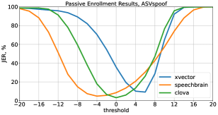
Figure 2: Results (in terms of JER, %) for passive enrollment with three types of speaker embeddings.

Embedding	ASVspoof	VoxCeleb
CLOVA	27.42	4.55
SpeechBrain	7.41	-
x-vector	70.64	8.86

Table 3: JERs (%) of different embeddings on the two evaluation sets. The threshold value is optimized individually. Since the training set for the SpeechBrain embedding extractor includes the VoxCeleb1 data, we do not evaluate it here.

8 Results for Passive Enrollment

The results of passive enrollment with varying thresholds are illustrated in Fig. 2 for the ASVspoof dataset for all three types of speaker embeddings. SpeechBrain yields lower JER than the other two embeddings for a wide range of thresholds. Performance becomes worse till 100% JER is beyond a certain range of threshold values applied on the similarity measures. For a certain lower value of the threshold, the number of predicted clusters is less, hence resulting in a high false alarm. Conversely, for a certain higher value of the threshold, the number of predicted clusters is very high and that leads to a high miss rate.

In our final experiment, we use the VoxCeleb dev data to set the thresholds (one per each embedding type). These thresholds then remain fixed on the evaluation part of ASVspoof and VoxCeleb data. The results in Table 3 indicate that SpeechBrain performs best on ASVspoof with a JER of 7.41%, while the performance is worst for the x-vector embedding extractor. This might be due to dataset mismatch leading to a threshold that fails to generalize from VoxCeleb on ASVspoof. Concerning the relative performance of CLOVA and x-vector, the former outperforms the latter by demonstrating better generalization ability on both datasets. Nevertheless, the best performances via grid search over different clustering thresholds (Fig. 2) indicate scope for improvement in passive enrollment.

All in all, the above findings are observations that serve as a baseline and future work on passive enrollment may start from here.

9 Conclusion

The aim of this work has been the creation of an accessible and reproducible entry point to address household speaker recognition tasks. Besides detailing the task and assumptions, we designed a public evaluation benchmark for both active and passive enrollment; and online and offline algorithms. From the various methods considered, the simple online update rule based on the weighted average of embeddings achieved competitive performance to offline algorithms. The simplicity and computationally cheap updates make it a viable solution for household speaker recognition.

Our planned future work includes (1) improving the baselines to improve domain robustness. For instance, it would be interesting to generalize existing domain adaptation methods to handle online data. (2) We also plan to analyze the online methods in terms of their sensitivity to the order of data. (3) Despite the promising preliminary results, it is also important to analyze the impact of the critical control parameters on the convergence properties of the algorithms. An important difference with generic speaker recognition tasks is that the model(s) are allowed to evolve with time which complicates analysis. Nonetheless, it is preferable to find principled alternatives over grid search. (4) Finally, we plan to include more methods, especially to the passive enrollment scenarios which we only slightly touched upon. We may also need new performance metrics for a more aligned comparison of active and passive scenarios.

10 Appendix

10.1 PLDA with spherical covariance $\equiv$ cosine scoring

Let $\boldsymbol{x}_{i,j}\in\mathbb{R}^{d}$ denote $j$th speaker embedding (observation) of speaker $i$. The two-covariance PLDA [14] assumes these observations to have been generated by a linear Gaussian model of the form

$$\boldsymbol{x}_{i,j}=\boldsymbol{\mu}+\boldsymbol{y}_{i}+\boldsymbol{\varepsilon}_{i,j},$$

where $\boldsymbol{\mu}$ is global mean of the embedding space, $\boldsymbol{y}_{i}$ is latent speaker identity variable with prior distribution $\boldsymbol{y}_{i}\sim\mathcal{N}(\boldsymbol{0},\boldsymbol{\mathrm{B}})$ and $\boldsymbol{\varepsilon}_{i,j}$ a residual with prior $\boldsymbol{\varepsilon}_{i,j}\sim\mathcal{N}(\boldsymbol{0},\boldsymbol{\mathrm{W}})$. The model is equivalently specified by the following distributions:

$$p(\boldsymbol{y}_{i}) =\mathcal{N}(\boldsymbol{y}_{i}|\boldsymbol{0},\boldsymbol{\mathrm{B}})$$ (2)

$$p(\boldsymbol{x}_{i,j}|\boldsymbol{y}_{i}) =\mathcal{N}(\boldsymbol{x}_{i,j}|\boldsymbol{\mu}+\boldsymbol{y}_{i},\boldsymbol{\mathrm{W}}).$$

The two matrices $\boldsymbol{\mathrm{B}}$ and $\boldsymbol{\mathrm{W}}$ model between- and within-speaker covariances, respectively. By imposing subspace structure on these matrices (rank $<d$) one may obtain other flavors of PLDA [15] as special cases. Here, we consider the highly-constrained case of spherical covariances,

$$\boldsymbol{\mathrm{B}} =\sigma_{\text{B}}^{2}\boldsymbol{\mathrm{I}}$$ (3)

$$\boldsymbol{\mathrm{W}} =\sigma_{\text{W}}^{2}\boldsymbol{\mathrm{I}},$$

where $\sigma_{\text{B}}^{2}$ and $\sigma_{\text{W}}^{2}$ are between-speaker and within-speaker variances and $\boldsymbol{\mathrm{I}}$ denotes an identity matrix.

For speaker comparison, the PLDA model (2) is used for computing log-likelihood ratio (LLR) score of same-speaker vs. different-speaker hypotheses for a pair of enrollment $(\boldsymbol{x}_{\text{e}})$ and test $(\boldsymbol{x}_{\text{t}})$ embeddings. For the null (same-speaker) hypothesis one assumes $\boldsymbol{x}_{\text{e}}$ and $\boldsymbol{x}_{\text{y}}$ to share common latent identity variable while for the alternative (different-speaker) hypothesis these latent factors are assumed to be different. While the interested reader may refer to details in [45, 46], the resulting LLR score can be written in closed form as

$$\ell=\boldsymbol{x}_{\text{e}}^{\mathsf{T}}\boldsymbol{\mathrm{P}}\boldsymbol{x}_{\text{t}}+\boldsymbol{x}_{\text{t}}^{\mathsf{T}}\boldsymbol{\mathrm{P}}\boldsymbol{x}_{\text{e}}+\boldsymbol{x}_{\text{e}}^{\mathsf{T}}\boldsymbol{\mathrm{Q}}\boldsymbol{x}_{\text{e}}+\boldsymbol{x}_{\text{t}}^{\mathsf{T}}\boldsymbol{\mathrm{Q}}\boldsymbol{x}_{\text{t}}+\boldsymbol{c}^{\mathsf{T}}(\boldsymbol{x}_{\text{t}}+\boldsymbol{x}_{\text{e}})+k,$$

where the matrices $\boldsymbol{\mathrm{P}}$, $\boldsymbol{\mathrm{Q}}$, the vector $\boldsymbol{c}$ and scalar $k$ depend only on the PLDA model parameters $(\boldsymbol{\mu},\boldsymbol{\mathrm{B}},\boldsymbol{\mathrm{W}})$. With the spherical covariance assumption (3), $\boldsymbol{\mathrm{P}}$ and $\boldsymbol{\mathrm{Q}}$ turn out to be scaled identity matrices too, say $\boldsymbol{\mathrm{P}}=\alpha\boldsymbol{\mathrm{I}}$, $\boldsymbol{\mathrm{Q}}=\beta\boldsymbol{\mathrm{I}}$. Further, the vector $\boldsymbol{c}=\gamma\boldsymbol{\mu}$ is scaled version of the mean.

We can now rewrite the LLR score as

$$\ell =\boldsymbol{x}_{\text{e}}^{\mathsf{T}}(\alpha\boldsymbol{\mathrm{I}})\boldsymbol{x}_{\text{t}}+\boldsymbol{x}_{\text{t}}^{\mathsf{T}}(\alpha\boldsymbol{\mathrm{I}})\boldsymbol{x}_{\text{e}}+\boldsymbol{x}_{\text{e}}^{\mathsf{T}}(\beta\boldsymbol{\mathrm{I}})\boldsymbol{x}_{\text{t}}+\boldsymbol{x}_{\text{t}}^{\mathsf{T}}(\beta\boldsymbol{\mathrm{I}})\boldsymbol{x}_{\text{e}}$$ (4)

$$+\gamma\boldsymbol{\mu}^{\mathsf{T}}(\boldsymbol{x}_{\text{e}}+\boldsymbol{x}_{\text{t}})+k$$

$$=2\alpha\boldsymbol{x}_{\text{e}}^{\mathsf{T}}\boldsymbol{x}_{\text{t}}+\beta(\|\boldsymbol{x}_{\text{e}}\|^{2}+\|\boldsymbol{x}_{\text{t}}\|^{2})+\gamma\boldsymbol{\mu}^{\mathsf{T}}(\boldsymbol{x}_{\text{e}}+\boldsymbol{x}_{\text{t}})+k.$$

We proceed by noting that subtracting an arbitrary global offset $\boldsymbol{b}\in\mathbb{R}^{d}$ from all speaker embeddings, $\boldsymbol{x}_{i,j}\leftarrow\boldsymbol{x}_{i,j}-\boldsymbol{b}$, preserves pairwise distances and angles between vectors and therefore retains the geometric structure of the speaker embedding space. This leads to an otherwise identical PLDA model but with global mean $\boldsymbol{\mu}-\boldsymbol{b}$. Therefore, by choosing $\boldsymbol{b}=\boldsymbol{\mu}$, the new model has a global mean $\boldsymbol{0}$ and (4) becomes

$$\ell=2\alpha\boldsymbol{x}_{\text{e}}^{\mathsf{T}}\boldsymbol{x}_{\text{t}}+\beta(\|\boldsymbol{x}_{\text{e}}\|^{2}+\|\boldsymbol{x}_{\text{t}}\|^{2})+k.$$

If both the enrollment and test embeddings are length-normalized ($\|\boldsymbol{x}_{\text{e}}\|=\|\boldsymbol{x}_{\text{t}}\|=1$), the score further simplies to

$$\ell=2\alpha\boldsymbol{x}_{\text{e}}^{\mathsf{T}}\boldsymbol{x}_{\text{t}}+2\beta+k,$$

which is an affine transform of the inner product $\boldsymbol{x}_{\text{e}}^{\mathsf{T}}\boldsymbol{x}_{\text{t}}$ (cosine score) between the enrollment and test embeddings. Thus, PLDA scoring with spherical covariance matrices and cosine scoring are mappable to one another through order-preserving transform and therefore present equivalent scoring rules.

10.2 Note on PLDA and many-to-many verification

Consider set-to-set speaker verification where a trial is represented by a pair of sets with arbitrary cardinalities: $\boldsymbol{\mathrm{X}}_{\text{e}}=\{\boldsymbol{x}_{\text{e},1},\dots,\boldsymbol{x}_{\text{e},N}\}$ and $\boldsymbol{\mathrm{X}}_{\text{t}}=\{\boldsymbol{x}_{t,1},\dots,\boldsymbol{x}_{\text{t},M}\}$, referred to as the enrollment and the test set, respectively.

Assuming that the observations are generated from the PLDA model with the latent identity variable, denoted by $\boldsymbol{y}$, the verification likelihood ratio can be written as a function of the posterior distributions of $\boldsymbol{y}$ [47]

$$\mathrm{LR}(\boldsymbol{\mathrm{X}}_{\text{e}},\boldsymbol{\mathrm{X}}_{\text{t}})=\frac{p(\boldsymbol{\mathrm{X}}_{\text{e}},\boldsymbol{\mathrm{X}}_{\text{t}}|\mathrm{same})}{p(\boldsymbol{\mathrm{X}}_{\text{e}},\boldsymbol{\mathrm{X}}_{\text{t}}|\mathrm{diff})}\\ =\int\frac{p(\boldsymbol{y}|\boldsymbol{\mathrm{X}}_{\text{e}})p(\boldsymbol{y}|\boldsymbol{\mathrm{X}}_{\text{t}})}{p(\boldsymbol{y})}\mathop{}\!\mathrm{d}\boldsymbol{y},$$ (5)

where the integral admits the closed-form expression. These posteriors can be seen to be Gaussian with the mean parameters depending only on the average of feature vectors:

$$p(\boldsymbol{y}|\boldsymbol{x}_{1},\dots,\boldsymbol{x}_{N})=\mathcal{N}(\boldsymbol{y}|\boldsymbol{m},\boldsymbol{\mathrm{\Sigma}}),$$

$$\boldsymbol{\mathrm{\Sigma}}=\left(\boldsymbol{\mathrm{B}}^{-1}+N\cdot\boldsymbol{\mathrm{W}}^{-1}\right)^{-1},$$

$$\boldsymbol{m}=N\cdot\boldsymbol{\mathrm{\Sigma}}\boldsymbol{\mathrm{W}}^{-1}\boldsymbol{c},$$

where $\boldsymbol{c}=\frac{1}{N}\sum_{i=1}^{N}\boldsymbol{x}_{i}$ is the centroid (average vector) of the set. One can see that the log-likelihood ratio can be computed even if both sets are represented implicitly by pairs of (centroid, cardinality):

$$\mathrm{LR}(\boldsymbol{\mathrm{X}}_{e},\boldsymbol{\mathrm{X}}_{t})\equiv\mathrm{LR}((\boldsymbol{c}_{e},N),(\boldsymbol{c}_{t},M)),$$ (6)

where $\boldsymbol{c}_{e}$ and $\boldsymbol{c}_{t}$ are the centroids of $\boldsymbol{\mathrm{X}}_{e}$ and $\boldsymbol{\mathrm{X}}_{t}$, respectively. The counts, $N$ and $M$, are known as the zero-order statistics.

It worth noting that embeddings averaging is a commonly used strategy for speaker verification in the case of multiple enrollment utterances [21]. And PLDA can be also seen as an instance of ‘‘centroid based’’ scoring, with a difference that the information about the set cardinality is preserved. Intuitively, the information about set cardinality allows to make judgments about uncertainty: the more vectors are in the set, the higher confidence of the mean estimate. The PLDA model has advantage of taking this information into account.

Let us now recall the centroid algorithm where the speakers are represented by centroids, and the centroids are updated by the exponential smoothing rule:

$$\boldsymbol{c}^{(t)}=\alpha\boldsymbol{x}^{(t)}+(1-\alpha)\boldsymbol{c}^{(t-1)}.$$

By direct substitution of the update rule back into itself, one can see that it corresponds to the weighted averaging:

$$\boldsymbol{c}^{(N)}=\sum_{i=1}^{N}p_{i}\boldsymbol{x}^{(t)}$$

$$p_{i}=\begin{cases}(1-\alpha)^{N-1}&\text{if $i=1$}\\ \alpha(1-\alpha)^{(N-i)}&\text{if $i>1$}\\ \end{cases}$$

with $\boldsymbol{c}^{(0)}=\boldsymbol{x}_{1}$.

Now, if one wants to use the updated centroid for verification against the test utterance $\boldsymbol{x}_{\text{test}}$, it is not immediately obvious how to define the zero-order statistic $n$ in $\mathrm{LR}((\boldsymbol{c}^{(N)},n),\boldsymbol{x}_{\text{test}})$, given by (6). For example, updating a centroid with a very small $\alpha\approx 0$ does not benefit from the information available after collecting several new data points. Therefore, setting $n$ with the number of collected embeddings would not be adequate.

Here we propose a heuristic to set the count parameter in the case of unequal weights. First, let us notice that if $\alpha=0$ or $\alpha=1$, this boils down to the single enrollment verification, that is, the input count is $1$. This corresponds to either $p_{1}=1$ or $p_{N}=1$ with other weights being zero. Also, if $p_{i}=1/N$ for all $i=1...N$, then the cardinality is $N$.

Noting that the entropy of the discrete uniform distribution $\boldsymbol{p}=[p_{1},p_{2},...,p_{N}]$ where $p_{i}=1/N$ equals to $\log N$, we calculate the zero-order statistic as

$$n=e^{\mathcal{H}(\boldsymbol{p})}.$$

where $\mathcal{H}(\boldsymbol{p})=-\sum_{i}p_{i}\log p_{i}$ is the entropy. Then, for the maximum entropy, achieved for the uniform distribution, $n=N$. At the same time, if one of the weights equals to $1$, then $n=1$, which is also consistent with the special case.

Another issue related to setting the zero-order statistic is discussed in studies [48, 49, 50] in the context of compensating apparently inadequate assumption of feature independence. The proposed solutions suggest to scale down zero-order statistics $n_{r}=r\cdot n$ with the recommended factor of $r=0.2-0.3$ [48, 13] or simply setting $n=1$ independently of the set cardinality [21]. The latter heuristic is nothing else than a commonly adopted recipe of embedding averaging.

10.3 VB clustering details

We assume that the extracted utterance embeddings were generated by the PLDA model with the full-rank speaker subspace in the form of two-covariance model [14]. This model, specified by (2), is parameterized by two matrices $\boldsymbol{\mathrm{B}}$ and $\boldsymbol{\mathrm{W}}$ interpreted as between- and within-speaker covariances. We assume the data have zero-mean.

We construct a finite mixture model for partitioning a set of embeddings $\boldsymbol{\mathrm{X}}=\{\boldsymbol{x}_{1},\dots,\boldsymbol{x}_{N}\}$ into $K$ clusters corresponding to individual speakers. The speakers are represented by Gaussians with a shared covariance matrix $\boldsymbol{\mathrm{W}}$ and speaker-specific latent mean vectors $\boldsymbol{\mathrm{Y}}=\{\boldsymbol{y}_{1},\dots,\boldsymbol{y}_{K}\}$.

Further, each embedding $\boldsymbol{x}_{i}$ is associated with a binary one-hot vector $\boldsymbol{z}_{i}$, whose components indicate whether this observation belongs to the corresponding mixture component. For instance, if the embedding $\boldsymbol{x}_{i}$ is generated from component $k$ then $z_{i,k}=1$ with other vector components equal to zero.

The latent variables $\boldsymbol{\mathrm{Z}}=\{\boldsymbol{z}_{1},\dots,\boldsymbol{z}_{N}\}$ are drawn independently from the categorical distributions governed by the mixing coefficients $\pi_{k}$:

$$p(\boldsymbol{\mathrm{Z}})=\prod_{i=1}^{N}\prod_{k=1}^{K}\pi_{k}^{z_{i,k}}$$

Conditioned on $\boldsymbol{\mathrm{Z}}$, the embeddings are assumed to be independently drawn from a speaker-specific Gaussian distribution so that

$$p(\boldsymbol{\mathrm{X}}|\boldsymbol{\mathrm{Y}},\boldsymbol{\mathrm{Z}})=\prod_{i=1}^{N}\prod_{k=1}^{K}\mathcal{N}(\boldsymbol{x}_{i}|\boldsymbol{y}_{k},\boldsymbol{\mathrm{W}})^{z_{i,k}}$$

We further modified the standard mixture model described above by introducing one extra label to present ‘background class’. To this end, we added one component to the mixture model that represents the marginal distribution of embeddings:

$$p(\boldsymbol{x})=\int p(\boldsymbol{x}|\boldsymbol{y})p(\boldsymbol{y})\mathop{}\!\mathrm{d}\boldsymbol{y}=\mathcal{N}(\boldsymbol{x}|\boldsymbol{0},\boldsymbol{\mathrm{B}}+\boldsymbol{\mathrm{W}})$$

This component, indexed as component $K+1$, corresponds to the embeddings which does not belong to any of $K$ clusters. In the context of household speaker recognition this component is intended to model all the unknown speakers (guests) at once, since discriminating those speakers is irrelevant to the task.

$$p(\boldsymbol{x}_{i}|\boldsymbol{\mathrm{Y}},\boldsymbol{z}_{i})=\begin{cases}\mathcal{N}(\boldsymbol{x}_{i}|\boldsymbol{0},\boldsymbol{\mathrm{B}}+\boldsymbol{\mathrm{W}})&\text{if $z_{i,K+1}=1$}\\ \mathcal{N}(\boldsymbol{x}_{i}|\boldsymbol{y}_{k},\boldsymbol{\mathrm{W}})^{z_{i,k}}&\text{otherwise}\\ \end{cases}$$

The clustering problem requires finding the most likely partition of the data, represented by $\boldsymbol{\mathrm{Z}}$. Following [13], we use variational Bayesian inference [34] to approximate the posterior distribution $p(\boldsymbol{\mathrm{Z}}|\boldsymbol{\mathrm{X}})\approx\prod_{i}q(\boldsymbol{z}_{i})$. Similar to the semi-supervised k-means clustering described above, posterior distribution $q(\boldsymbol{z})$ for a subset of labeled data points are initialized by one-hot representations of their known labels and kept fixed during inference. After the convergence, the inferred cluster assignments can be found as $k_{i}^{*}=\arg\max_{k}q(\boldsymbol{z_{i,k}})$. Detailed derivations and the update rules can be found in [13].

Finally, the joint distribution of all of the random variables is given by

$$p(\boldsymbol{\mathrm{X}},\boldsymbol{\mathrm{Y}},\boldsymbol{\mathrm{Z}})=p(\boldsymbol{\mathrm{X}}|\boldsymbol{\mathrm{Y}},\boldsymbol{\mathrm{Z}})p(\boldsymbol{\mathrm{Y}})p(\boldsymbol{\mathrm{Z}}).$$

The clustering problem requires finding the most likely partition of the data, represented by $\boldsymbol{\mathrm{Z}}$. This can be formulated as finding the most likely partition $\boldsymbol{\mathrm{Z}}^{*}=\arg\max_{\boldsymbol{\mathrm{Z}}}p(\boldsymbol{\mathrm{Z}}|\boldsymbol{\mathrm{X}})$ where $p(\boldsymbol{\mathrm{Z}}|\boldsymbol{\mathrm{X}})=\int p(\boldsymbol{\mathrm{Z}}|\boldsymbol{\mathrm{Y}},\boldsymbol{\mathrm{X}})\mathop{}\!\mathrm{d}\boldsymbol{\mathrm{Y}}$ is the clustering (partition) posterior distribution. Since direct optimization of this objective is intractable due to vast combinatorial search space, one has to resort to available approximation techniques. We use variational Bayesin inference [34] to approximate the joint posterior $q(\boldsymbol{\mathrm{Z}},\boldsymbol{\mathrm{Y}})\approx p(\boldsymbol{\mathrm{Z}},\boldsymbol{\mathrm{Y}}|\boldsymbol{\mathrm{X}})$ assuming that the approximate posterior is factorizes as $q(\boldsymbol{\mathrm{Z}},\boldsymbol{\mathrm{Y}})=q(\boldsymbol{\mathrm{Z}})q(\boldsymbol{\mathrm{Y}})$. We use variational inference because is often much faster than Monte-Carlo based [51] or greedy algorithms [52].

Following [13], we search for such $q(\boldsymbol{\mathrm{Z}})$ and $q(\boldsymbol{\mathrm{Y}})$ that maximize the weighted evidence lower bound (ELBO) augmented with a pair of scaling factors $F_{A}$ and $F_{B}$:

$$\mathcal{L}(q(\boldsymbol{\mathrm{Z}}),q(\boldsymbol{\mathrm{Y}}))=F_{A}\cdot\mathbb{E}_{q(\boldsymbol{\mathrm{Z}})q(\boldsymbol{\mathrm{Y}})}[\log p(\boldsymbol{\mathrm{X}}|\boldsymbol{\mathrm{Y}},\boldsymbol{\mathrm{Z}})]$$

$$-F_{B}\cdot\mathrm{KL}(q(\boldsymbol{\mathrm{Y}})\|p(\boldsymbol{\mathrm{Y}}))-\mathrm{KL}(q(\boldsymbol{\mathrm{Z}})\|p(\boldsymbol{\mathrm{Z}})).$$

Here, $\mathbb{E}_{q}[\cdot]$ denotes expectation with respect to $q$ and $\mathrm{KL}(\cdot\|\cdot)$ is the Kullback-Leibler divergence [34]. Despite that the theoretically correct variational Bayesian inference assumes $F_{A}=F_{B}=1$, tuning the values of these scaling factors helps to compensate for wrong model assumptions of statistical independence and to improve the clustering performance. For a more in-depth discussion of their interpretations, please refer to [13].

The assumption of factorized posterior leads to the inference algorithm consisting of iterative updates of factors $q(\boldsymbol{\mathrm{Z}})$ and $q(\boldsymbol{\mathrm{Y}})$, with each update having a closed-form solution. Similar to the semi-supervised k-means clustering described above, posterior distribution $q(\boldsymbol{z})$ for a subset of labeled data points are initialized by one-hot representations of their known labels and kept fixed during inference. After the convergence, the inferred cluster assignments can be found as $k_{i}^{*}=\arg\max_{k}q(\boldsymbol{z_{i,k}})$. Detailed derivations and the update rules can be found in [13].

11 References

References

- [1] Long Chen, Venkatesh Ravichandran and Andreas Stolcke ‘‘Graph-based Label Propagation for Semi-Supervised Speaker Identification’’ In CoRR abs/2106.08207, 2021 URL: https://arxiv.org/abs/2106.08207
- [2] Zhenning Tan et al. ‘‘Improving Speaker Identification for Shared Devices by Adapting Embeddings to Speaker Subsets’’ In ASRU, 2021, pp. 1124–1131
- [3] Craig S. Greenberg et al. ‘‘Two decades of speaker recognition evaluation at the national institute of standards and technology’’ In Computer Speech and Language 60, 2020, pp. 101032 DOI: https://doi.org/10.1016/j.csl.2019.101032
- [4] A. Nagrani, J. Chung and A. Zisserman ‘‘VoxCeleb: A Large-Scale Speaker Identification Dataset’’ In Interspeech, 2017, pp. 2616–2620
- [5] J. Chung, A. Nagrani and A. Zisserman ‘‘VoxCeleb2: deep Speaker Recognition’’ In Interspeech, 2018, pp. 1086–1090
- [6] Brecht Desplanques, Jenthe Thienpondt and Kris Demuynck ‘‘ECAPA-TDNN: Emphasized Channel Attention, Propagation and Aggregation in TDNN Based Speaker Verification’’ In Interspeech, 2020, pp. 3830–3834
- [7] D. Snyder et al. ‘‘Speaker Recognition for Multi-speaker Conversations Using X-vectors’’ In ICASSP, 2019, pp. 5796–5800
- [8] Baochen Sun, Jiashi Feng and Kate Saenko ‘‘Return of Frustratingly Easy Domain Adaptation’’ In AAAI, 2016, pp. 2058–2065
- [9] Kong Aik Lee, Qiongqiong Wang and Takafumi Koshinaka ‘‘The CORAL+ Algorithm for Unsupervised Domain Adaptation of PLDA’’ In ICASSP, 2019, pp. 5821–5825
- [10] Md Jahangir Alam, Gautam Bhattacharya and Patrick Kenny ‘‘Speaker Verification in Mismatched Conditions with Frustratingly Easy Domain Adaptation ’’ In Odyssey, 2018, pp. 176–180
- [11] Pierre-Michel Bousquet and Mickael Rouvier ‘‘On Robustness of Unsupervised Domain Adaptation for Speaker Recognition’’ In Interspeech, 2019, pp. 2958–2962
- [12] Dengyong Zhou et al. ‘‘Learning with Local and Global Consistency’’ In NIPS, 2003, pp. 321–328
- [13] Mireia Díez et al. ‘‘Analysis of Speaker Diarization Based on Bayesian HMM With Eigenvoice Priors’’ In IEEE ACM Trans. Audio Speech Lang. Process. 28, 2020, pp. 355–368
- [14] Niko Brümmer and Edward Villiers ‘‘The speaker partitioning problem’’ In Odyssey, 2010, pp. 34
- [15] Aleksandr Sizov, Kong-Aik Lee and Tomi Kinnunen ‘‘Unifying Probabilistic Linear Discriminant Analysis Variants in Biometric Authentication’’ In S+SSPR, Joint IAPR International Workshop 8621, Lecture Notes in Computer Science Springer, 2014, pp. 464–475
- [16] Xin Wang et al. ‘‘ASVspoof 2019: A large-scale public database of synthesized, converted and replayed speech’’ In Computer Speech and Language 64, 2020, pp. 101114 URL: https://www.sciencedirect.com/science/article/pii/S0885230820300474
- [17] P. A.. and A. Malagaonkar ‘‘Verification effectiveness in open-set speaker identification’’ In ICVISP 153.5, 2006, pp. 618–624
- [18] Raymond W.. Ng, Xuechen Liu and Pawel Swietojanski ‘‘Teacher-Student Training for Text-Independent Speaker Recognition’’ In IEEE SLT Workshop, 2018, pp. 1044–1051
- [19] Shuai Wang et al. ‘‘Knowledge Distillation for Small Foot-print Deep Speaker Embedding’’ In ICASSP, 2019, pp. 6021–6025
- [20] Joon Son Chung et al. ‘‘VoxSRC 2019: The first VoxCeleb Speaker Recognition Challenge’’ In CoRR abs/1912.02522, 2019
- [21] Padmanabhan Rajan et al. ‘‘From single to multiple enrollment i-vectors: Practical PLDA scoring variants for speaker verification’’ In Digital Signal Processing 31, 2014, pp. 93–101 DOI: https://doi.org/10.1016/j.dsp.2014.05.001
- [22] Chang Zeng et al. ‘‘Attention Back-end for Automatic Speaker Verification with Multiple Enrollment Utterances’’ In CoRR abs/2104.01541, 2021 URL: https://arxiv.org/abs/2104.01541
- [23] Z. Bai and X. Zhang ‘‘Speaker recognition based on deep learning: An overview’’ In Neural Networks 140, 2021, pp. 65–99
- [24] Arsha Nagrani et al. ‘‘VoxSRC 2020: The Second VoxCeleb Speaker Recognition Challenge’’ In CoRR abs/2012.06867, 2020
- [25] Mahesh Kumar Nandwana et al. ‘‘The VOiCES from a Distance Challenge 2019: Analysis of Speaker Verification Results and Remaining Challenges’’ In Odyssey, 2020, pp. 165–170
- [26] Jiankang Deng et al. ‘‘ArcFace: Additive Angular Margin Loss for Deep Face Recognition’’ In CVPR, 2019
- [27] Joon Son Chung et al. ‘‘In defence of metric learning for speaker recognition’’ In Interspeech, 2020, pp. 2977–2981
- [28] David Snyder et al. ‘‘X-Vectors: Robust DNN Embeddings for Speaker Recognition’’ In ICASSP, 2018, pp. 5329–5333
- [29] Hossein Zeinali et al. ‘‘BUT System Description to VoxCeleb Speaker Recognition Challenge 2019’’ In CoRR abs/1910.12592, 2019 URL: http://arxiv.org/abs/1910.12592
- [30] Hagai Aronowitz ‘‘Compensating Inter-Dataset Variability in PLDA Hyper-Parameters for Robust Speaker Recognition’’ In Odyssey, 2014
- [31] Robert Goodell Brown ‘‘Smoothing, Forecasting and Prediction of Discrete Time Series’’ Englewood-Cliffs, NJ: Prentice-Hall, 1963
- [32] Xiaojin Zhu ‘‘Semi-Supervised Learning Literature Survey’’, 2005 URL: http://pages.cs.wisc.edu/~jerryzhu/pub/ssl_survey.pdf
- [33] A.. Jain, M.. Murty and P.. Flynn ‘‘Data clustering: a review’’ In ACM Comput. Surv. 31.3 New York, NY, USA: ACM, 1999, pp. 264–323
- [34] C.M. Bishop ‘‘Pattern Recognition and Machine Learning’’ New York: Springer Science+Business Media, LLC, 2006
- [35] A. Corduneanu and Christopher Bishop ‘‘Variational Bayesian Model Selection for Mixture Distributions’’ In AISTATS, 2001, pp. 27–34 URL: https://www.microsoft.com/en-us/research/publication/variational-bayesian-model-selection-for-mixture-distributions/
- [36] Dengyong Zhou et al. ‘‘Learning with Local and Global Consistency’’ In NIPS, 2003, pp. 321–328
- [37] K. Okabe, T. Koshinaka and K. Shinoda ‘‘Attentive Statistics Pooling for Deep Speaker Embedding’’ In Interspeech, 2018, pp. 2252–2256
- [38] F. Wang et al. ‘‘Additive Margin Softmax for Face Verification’’ In IEEE Signal Processing Letters 25.7, 2018, pp. 926–930 DOI: 10.1109/LSP.2018.2822810
- [39] Mirco Ravanelli et al. ‘‘SpeechBrain: A General-Purpose Speech Toolkit’’, 2021 arXiv:2106.04624 [eess.AS]
- [40] Hee Soo Heo et al. ‘‘Clova baseline system for the VoxCeleb Speaker Recognition Challenge 2020’’ In arXiv preprint arXiv:2009.14153, 2020
- [41] Kaiming He et al. ‘‘Deep Residual Learning for Image Recognition’’ In CVPR, 2016, pp. 770–778
- [42] David A. Leeuwen, Niko Brummer and Albert Swart ‘‘A comparison of linear and non-linear calibrations for speaker recognition’’ In Odyssey, 2014
- [43] Trevor Hastie, Robert Tibshirani and Jerome Friedman ‘‘The Elements of Statistical Learning’’, Springer Series in Statistics New York, NY, USA: Springer New York Inc., 2001
- [44] Neville Ryant et al. ‘‘The Second DIHARD Diarization Challenge: Dataset, Task, and Baselines’’ In Interspeech, 2019, pp. 978–982
- [45] Lukás Burget et al. ‘‘Discriminatively trained Probabilistic Linear Discriminant Analysis for speaker verification’’ In ICASSP, 2011, pp. 4832–4835
- [46] Johan Rohdin, Sangeeta Biswas and Koichi Shinoda ‘‘Discriminative PLDA training with application-specific loss functions for speaker verification’’ In Odyssey, 2014, pp. 26–32
- [47] Jesús Villalba, Niko Brümmer and Najim Dehak ‘‘Tied Variational Autoencoder Backends for i-Vector Speaker Recognition’’ In Interspeech, 2017, pp. 1004–1008
- [48] Themos Stafylakis et al. ‘‘Compensation for inter-frame correlations in speaker diarization and recognition’’ In ICASSP, 2013, pp. 7731–7735
- [49] Alan McCree, Gregory Sell and Daniel Garcia-Romero ‘‘Extended Variability Modeling and Unsupervised Adaptation for PLDA Speaker Recognition’’ In Interspeech, 2017, pp. 1552–1556
- [50] Alan McCree, Gregory Sell and Daniel Garcia-Romero ‘‘Speaker Diarization Using Leave-One-Out Gaussian PLDA Clustering of DNN Embeddings’’ In Interspeech, 2019, pp. 381–385
- [51] Christophe Andrieu et al. ‘‘An Introduction to MCMC for Machine Learning’’ In Mach. Learn. 50.1-2, 2003, pp. 5–43 DOI: 10.1023/A:1020281327116
- [52] Anna Silnova et al. ‘‘Probabilistic Embeddings for Speaker Diarization’’ In Odyssey, 2020, pp. 24–31