Chromatic $k$-Nearest Neighbor Queries

Abstract

Let $P$ be a set of $n$ colored points. We develop efficient data structures that store $P$ and can answer chromatic $k$-nearest neighbor ($k$-NN) queries. Such a query consists of a query point $q$ and a number $k$, and asks for the color that appears most frequently among the $k$ points in $P$ closest to $q$. Answering such queries efficiently is the key to obtain fast $k$-NN classifiers. Our main aim is to obtain query times that are independent of $k$ while using near-linear space.

We show that this is possible using a combination of two data structures. The first data structure allow us to compute a region containing exactly the $k$-nearest neighbors of a query point $q$, and the second data structure can then report the most frequent color in such a region. This leads to linear space data structures with query times of $O(n^{1/2}\log n)$ for points in $\mathbb{R}^{1}$, and with query times varying between $O(n^{2/3}\log^{2/3}n)$ and $O(n^{5/6}\operatorname{polylog}n)$, depending on the distance measure used, for points in $\mathbb{R}^{2}$. Since these query times are still fairly large we also consider approximations. If we are allowed to report a color that appears at least $(1-\varepsilon)f^{*}$ times, where $f^{*}$ is the frequency of the most frequent color, we obtain a query time of $O(\log n+\log\log_{\frac{1}{1-\varepsilon}}n)$ in $\mathbb{R}^{1}$ and expected query times ranging between $\tilde{O}(n^{1/2}\varepsilon^{-3/2})$ and $\tilde{O}(n^{1/2}\varepsilon^{-5/2})$ in $\mathbb{R}^{2}$ using near-linear space (ignoring polylogarithmic factors).

1 Introduction

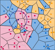
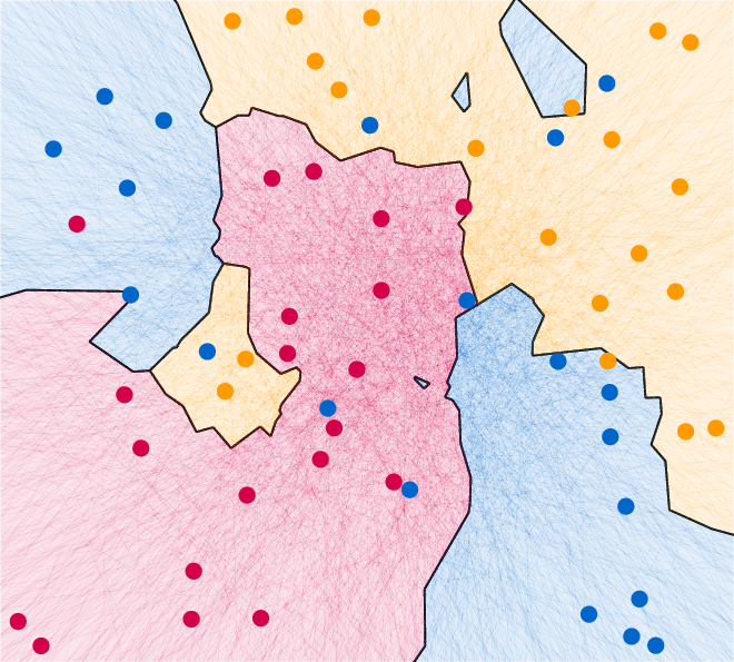
Figure 1: (left) A set of input points from three different classes (colors). The class of a query point $q$ is determined by the labels of its $k$ nearest neighbors (with $k=7$ as shown here $q$ is classified as red). (middle) The color partition for $k=1$. (right) The color partition for $k=3$.

One of the most popular approaches for classification problems is to use a $k$-Nearest Neighbor ($k\text{-NN}$) classifier [4, 17, 26, 30]. In a $k\text{-NN}$ classifier the predicted class of a query item $q$ is taken to be the most frequently appearing class among the $k$ items most similar to $q$. One can model this as a geometric problem in which the input items are represented by a set $P$ of $n$ colored points in $\mathbb{R}^{d}$: the color of the points represents their class, and the distance between points measures their similarity. The goal is then to store $P$ so that one can efficiently find the color (class) $c^{*}$ most frequently occurring among the $k$ points in $P$ closest to a query point $q$. See Figure 1(left). We refer to such queries as chromatic $k\text{-NN}$ queries. To answer such queries, $k\text{-NN}$ classifiers often store $P$ in, e.g., a kd-tree and answer queries by explicitly reporting the $k$ points closest to $q$, scanning through this set to compute the most frequently occurring color [4]. Unfortunately, for many distance measures (including the Euclidean distance) such an approach has no guarantees on the query time other than the trivial $O(n)$ time bound. See Figure 2 for an illustration. Even assuming that the dependency on $n$ during the query time is small (e.g. when the points are nicely distributed [24]), the approach requires $\Theta(k)$ time to explicitly process all $k$ points closest to $q$, whereas the desired output is only a single value: the most frequently appearing color. Hence, our main goal is to design a data structure to store $P$ that has sublinear query time in terms of both $n$ and $k$, while still using only small space. We focus our attention on the $L_{2}$ (Euclidean) distance, and the $L_{\infty}$ distance metrics. Most of our ideas extend to more general distance measures and higher dimensions as well. However, already in the restricted settings presented here, designing data structures that provide guarantees on the space and query time turns out to be a challenging task.

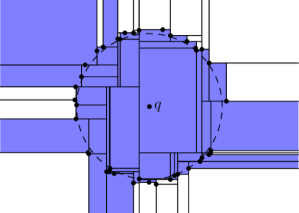
Figure 2: An example configuration in which querying a kd-tree for the $k$ nearest neighbors (in terms of the Euclidean distance) may visit a linear number of cells (shown in blue).

If the value $k$ is fixed in advance, one possible solution is to build the $k^{\mathrm{th}}$-order Voronoi diagram $\mathit{Vor}_{k}(P)$ of $P$, and preprocess it for point location queries. The $k^{\mathrm{th}}$-order Voronoi diagram is a partition of $\mathbb{R}^{d}$ into maximal cells for which all points in a cell (a Voronoi region) $V_{k,P}(S)$ have the same set $S$ of $k$ closest points from $P$. Hence, in each Voronoi region there is a fixed color that occurs most frequently among $S$. See Figure 1(right) for an illustration. By storing $\mathit{Vor}_{k}(P)$ in a data structure for efficient (i.e. $O(\log n)$ time) point location queries we can also answer chromatic $k\text{-NN}$ queries efficiently. However, unfortunately $\mathit{Vor}_{k}(P)$ may have size $\Theta(k(n-k))$ [32] (for points in $\mathbb{R}^{2}$ and the $L_{2}$ distance). For other $L_{m}$ distances the diagram is similarly large [34, 8]. Hence, we are interested in solutions that use less, preferably near-linear, space.

The only result on the theory of chromatic $k\text{-NN}$ queries that we are aware of is that of Mount et al. [38]. They study the problem in the case that we measure distance using the Euclidean metric and that the number of colors $c$, as well as the parameter $k$, are small constants. Mount et al.state that it is unclear how to obtain a query time independent of $k$, and instead analyze the query times in terms of the chromatic density $\rho$ of a query $q$. The chromatic density is a term depending on the distance from the query point $q$ to the $k^{\mathrm{th}}$ nearest neighbor of $q$, and the distance from $q$ to the first point at which the answer of the query would change (e.g. the $(k+t)^{\mathrm{th}}$ nearest neighbor of $q$ for some $t>0$). The intuition is that if many points near $q$ have the same color, queries should be easier to answer than when there are multiple colors with roughly the same number of points. The chromatic density term models this. Their main result is a linear space data structure for points in $\mathbb{R}^{d}$ that supports $O(\log^{2}n+(1/\rho)^{d}\log(1/\rho))$ time queries. We aim for bounds only in terms of combinatorial properties (i.e. $n$, $c$, and $k$) and allow the number of colors, as well as the parameter $k$, to depend on $n$. Our results are particularly relevant when $k$ and $c$ are large compared to $n$.

Our approach.

Our main idea is to answer a query in two steps. (1) We identify a region $\mathcal{D}^{k}_{m}(q)$ that contains exactly the set $k\text{-NN}_{m}(q)$ of the $k$ sites closest to $q$ according to distance metric $L_{m}$. (2) We then find the mode color $c^{*}$; that is, the most frequently occurring color among the points in the region $\mathcal{D}^{k}_{m}(q)$. This way, we never have to explicitly enumerate the set $k\text{-NN}_{m}(q)$. We will design separate data structures for these two steps. Our data structure for step (1) will find the smallest metric disk $\mathcal{D}^{k}_{m}(q)$ containing $k\text{-NN}_{m}(q)$ centered at $q$. We refer to such a query as an range finding query. If the distance used is clear from the context we may write $k\text{-NN}(q)$ and $\mathcal{D}^{k}(q)$ instead.

Range mode queries.

The data structure in step (2) answers so-called range mode queries. For these data structures we exploit and extend the result of Chan et al. [12]. They show an array $A$ with $n$ entries can be stored in a linear space data structure that allows reporting the mode of a query range (interval) $A[i..j]$ in $O(n^{1/2})$ time. Furthermore, points in $\mathbb{R}^{d}$ can be stored in $O(n\operatorname{polylog}n+r^{2d})$ space so that range mode queries with axis-aligned orthogonal ranges can be answered in $O((n/r)\operatorname{polylog}n)$ time. Here, $r\in[1,n]$ is a user-choosable parameter. In particular, setting $r=\lceil n^{1/2d}\rceil$ yields an $O(n\operatorname{polylog}n)$ space solution with $O(n^{1-1/2d}\operatorname{polylog}n)$ query time. Range mode queries with halfspaces can be answered in $O((n/r)^{1-1/d^{2}}+\operatorname{polylog}n)$ time using $O(nr^{d-1})$ space [12]. Range mode queries in arrays have also been considered in an approximate setting [9]. The goal is then to report an element that appears sufficiently often in the range.

Dimension	Metric	Preprocessing time	Space	Query time
$d=1$	$L_{m}$	$O(n^{3/2}\log n)$	$O(n)$	$O(n^{1/2}\log n)$
$d=2$	$L_{m}$	$\tilde{O}(n^{2/(4+\delta)})$	$O(n)$	$\tilde{O}(n^{1-1/(12+3\delta)})$
$d\geq 3$	$L_{m}$	$\tilde{O}(n^{2-1/d}+n^{1+d/(2d-2+\delta)})$	$O(n)$	$\tilde{O}(n^{1-1/((d+1)(2d-2+\delta))})$
$d\geq 2$	$L_{\infty}$	$O(n^{1+d/(d+1)})$	$O(n)$	$O(n^{1-1/(d+1)+\delta})$
		$\tilde{O}(n^{1+d/(d+1)})$	$O(n\log^{d-1}n)$	$O((n\log^{d-1}n)^{1-1/(d+1)})$
	$L_{2}$	$\tilde{O}(n^{2-1/d}+n^{1+d/(d+1)})^{*}$	$O(n)$	$\tilde{O}(n^{1-(d-1)/d(d+1)})$

Table 1: Our results for exact chromatic $k$-nearest neighbors problems. Bounds marked with ^∗ are expected bounds. The general $L_{m}$ metric bounds hold for $m=O(1)$.

Results and organization.

Refer to Table 1 for an overview of our exact solutions. We first consider the problem for $n$ points in $\mathbb{R}^{1}$. In this setting, we develop an optimal linear space data structure that can find $\mathcal{D}^{k}_{m}(q)$ in $O(\log n)$ time, for any $m\geq 1$ (Section 2.1). We then use Chan et al. [12]’s data structure to report the mode color in $\mathcal{D}^{k}_{m}(q)$. Since we present all of our data structures in the pointer machine model augmented with real-valued arithmetic, this yields an $O(n^{1/2}\log n)$ time query algorithm. There is a conditional $\Omega(n^{1/2-\delta})$ lowerbound for chromatic $k\text{-NN}$ queries using linear space and $O(n^{3/2})$ preprocessing time (refer to Section 5) so this result is likely near-optimal. In Section 3 we present our data structure for finding $\mathcal{D}^{k}_{m}(q)$ in $\mathbb{R}^{2}$. For the $L_{\infty}$ metric we show that we can essentially find $\mathcal{D}^{k}_{m}(q)$ using a binary search on the radius of the disk, and thus there is a simple $O(n\log n)$ size data structure that allows us to find the range $\mathcal{D}^{k}(q)$ in $O(\log^{2}n)$ time (or $O(n^{\delta})$ time, for an arbitrarily small $\delta>0$, in case of a linear space structure). For the $L_{2}$ metric, we can no longer easily access a discrete set of candidate radii. It is tempting to therefore replace the binary search by a parametric search [37, 36]. However, the basic such approach squares the $\tilde{O}(n^{1/2})$ time required to solve the decision problem and is thus not applicable. The full strategy requires a way to generate independent comparisons; typically by designing a parallel decision algorithm [37]. Neither task is straightforward to achieve. Instead, we show that we can directly adapt the query algorithm for answering semi-algebraic range queries [3] (essentially the decision algorithm in the approach sketched above) to find $\mathcal{D}^{k}_{2}(q)$ in $O(n^{1/2}\operatorname{polylog}n)$ time. Unfortunately, the final query time for chromatic $k\text{-NN}$ queries is dominated by the $O(n^{5/6}\operatorname{polylog}n)$ time range mode queries, for which we use a slight variation of the data structure of Chan et al. [12]. We briefly discuss these results in Section 4, We do show that the data structure can be constructed in $O(n^{5/3})$ expected time, rather than the straightforward $O(n^{2})$ time implementation that directly follows from the description of Chan et al.. For the $L_{\infty}$ metric we can answer range mode queries in $O(n^{3/4}\operatorname{polylog}n)$ time using Chan et al.’s data structure for orthogonal ranges. However, we show that we can exploit that the ranges are squares and use a cutting-based approach (similar to the one used for the $L_{2}$ distance) to answer queries in $O(n^{2/3}\log^{2/3}n)$ time instead. If we wish to reduce the space from $O(n\log n)$ to linear the query time becomes $O(n^{2/3+\delta})$.

Since the query times are still rather large, we then turn our attention to approximations; refer to Table 2 for an overview. If $f^{*}$ is the frequency of the mode color among $k\text{-NN}(q)$ then our data structures may return a color that appears at least $(1-\varepsilon)f^{*}$ times. In case of the $L_{2}$ distance our data structure presented in Section 6 now achieves roughly $\tilde{O}(n^{1/2}\varepsilon^{-3/2})$ query time, where the $\tilde{O}$ notation hides polylogarithmic factors of $n$ and $\varepsilon$. The main idea is that approximate levels in the arrangement of distance functions have relatively low complexity, and thus we can store them to efficiently answer approximate range mode queries. We show how to generalize our results to higher dimensions and other distance metrics in Section 7.

Dimension	Metric	Preprocessing time	Space	Query time
$d=1$	$L_{m}$	$O(n\log_{\frac{1}{1-\varepsilon}})$	$O(n\varepsilon^{-1})$	$O(\log n+\log\log_{\frac{1}{1-\varepsilon}}n)$
$d=2$	$L_{\infty}$	$\tilde{O}(n\varepsilon^{-6})^{*}$	$\tilde{O}(n\varepsilon^{-6})$	$\tilde{O}(n^{1/2}\varepsilon^{-5/2})^{*}$
	$L_{2}$	$\tilde{O}(n^{1+\delta}+n\varepsilon^{-7})^{*}$	$\tilde{O}(n\varepsilon^{-4})$	$\tilde{O}(n^{1/2}\varepsilon^{-3/2})^{*}$

Table 2: Our results for the approximate chromatic $k$-nearest neighbors problems. Complexities marked with ^∗ are expected bounds.

2 The one-dimensional problem

In this section we consider the case where $P$ is a set of $n$ points in $\mathbb{R}^{1}$. In this case all $L_{m}$-distance metrics with $m\geq 1$ are the same, i.e. $L_{m}(a,b)=|a-b|$. We develop a linear space data structure supporting queries in $O(n^{1/2}\log n)$ time. Building the data structure will take $O(n^{3/2})$ time. We follow the general two-step approach sketched in Section 1. As we show in Section 2.1 there is an optimal, linear-space data structure with which we can find $\mathcal{D}^{k}(q)$ in $O(\log n)$ time, even if $k$ is part of the query. As we then briefly describe in Section 2.2 we can directly use the data structure by Chan et al. [12] to find the mode color of the points in $\mathcal{D}^{k}(q)$ in $O(n^{1/2}\log n)$ time.

2.1 Range finding queries

Given a set $P$ of $n$ points in $\mathbb{R}^{1}$, we wish to store $P$ so that given a query, consisting of a point $q\in\mathbb{R}^{1}$ and a natural number $k$, we can efficiently find the $k^{\mathrm{th}}$ furthest point from $q$, and thus $\mathcal{D}^{k}_{m}(q)$. We show that by storing $P$ in sorted order in an appropriate binary search tree, we can answer such queries in $O(\log n)$ time. To this end, we first consider answering so called rank queries on a ordered set, represented by a pair of binary search trees. This turns out to be the crucial ingredient in the data structure.

Rank queries.

Let $R\cup B$ be an ordered set of elements, and let $T_{R}$ be a be a binary search tree whose internal nodes store the elements from $R$, and in which each node is annotated with the number of elements in that subtree. Similarly, let $T_{B}$ be a binary search tree storing $B$. We now show how, given an natural number $k$, we can find the element among $R\cup B$ with rank $k$ (i.e. the $k^{\mathrm{th}}$ smallest element), in $O(0pt(T_{R})+0pt(T_{B}))$ time, where $0pt(T)$ denotes the height of tree $T$.

Let $r$ be the root of $T_{R}$, and let $R^{<}$ and $R^{>}$ be the subsets of $R$ with elements smaller and larger than the root, respectively. We define the root $b$ of $T_{B}$, and $B^{<}$ and $B^{>}$ analogously. Assume without loss of generality that $r>b$, and let $\ell=|B^{<}|+|R^{<}|+1$.

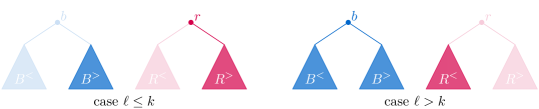
Figure 3: We have $b<r$ so the rank of $r$ is at least $\ell=|B^{<}|+|R^{<}|+1$. This gives two cases, depending on the relation between $\ell$ and $k$. In either case we decrease the height of one tree.

If $\ell\leq k$

then the item that we search for is not in $B^{<}$, $R^{<}$, or $\{b\}$. Hence, we can discard $T_{B^{<}}$, $T_{R^{<}}$, and the blue root $b$, and recursively search for the element with rank $k-\ell$ in the set $B^{>}\cup(R^{>}\cup\{r\})$. We can represent this set using $T_{B^{>}}$ and the binary search tree with root $r$ that has a leaf as its left subtree, and $T_{R^{>}}$ as its right subtree. See Figure 3.

If $\ell>k$

then the item that we search for is not in $R^{>}\cup\{r\}$, since the rank of $r$ is at least $\ell$. Hence, we can discard $r$ and $R^{>}$ and recursively search for the element of rank $k$ in $B\cup R^{<}$. This set can be represented by the pair of binary search trees $T_{B}$, $T_{R^{<}}$.

We continue the search until one of the trees is a leaf. We can then trivially use the size annotations to find the element of rank $k$ in the other tree $T$ in $O(0pt(T))$ time.

Since each node stores the subtree size, we can compute $\ell$, and thus determine in which case we are in constant time. In the first case, we reduce the height of $T_{B}$ by one. In the second case we reduce the height of $T_{R}$ by one. Hence, after at most $0pt(T_{B})+0pt(T_{R})$ rounds, one of the trees is a leaf. Note that during this process the roles of $R$ and $B$ may switch (depending on the ordering of the elements stored at their roots), but this does not affect the running time. We thus obtain:

Lemma 2.1.

Let $T_{B}$ and $T_{R}$ be two binary search trees with size annotations, and let $k$ be a natural number. We can compute the element of rank $k$ among $B\cup R$ in $O(0pt(T_{B})+0pt(T_{R}))$ time.

An optimal data structure for computing $\mathcal{D}^{k}(q)$.

We store $P$ in a balanced binary search tree $T_{P}$ with subtree-size annotations, so that we can: (i) search for the element of rank $k$, i.e. the $k$ smallest element, and (ii) given a query value $q\in\mathbb{R}^{1}$ we can split the tree at $q$ in $O(\log n)$ time. We can implement $T_{P}$ using e.g. a red black tree [42] (although with some care even a simple static balanced binary search tree will suffice). We will use the split operations only to answer queries; so we use path copying in this operation, so that we can still access the original tree once a query finishes [40]. The data structure uses $O(n)$ space, and can be built in $O(n\log n)$ time.

Given a query $(q,k)$ the main idea is now to split $T_{P}$ into two trees $T_{P^{<}}$ and $T_{P^{\geq}}$, where $P^{<}\subseteq P$ is the set of points left of $q$ and $P^{\geq}=P\setminus P^{<}$ is the remaining set of points right of $q$ (or coinciding with $q$). Observe that in these two trees, the points are actually ordered by distance to $q$ (albeit for $T_{P^{<}}$ the points are stored in decreasing order while the points in $T_{P^{\geq}}$ are stored in increasing order). So, we can essentially use the procedure from Lemma 2.1 on the trees $T_{P^{<}}$ and $T_{P^{\geq}}$ to find the point in $P^{\leq}\cup P^{>}$ with rank $k$ (according to the “by distance to $q$”-order). The only difference with the algorithm as described above is that for $T_{P^{<}}$ the roles of the left and right subtree are reversed. Splitting $T$ into $T_{P^{<}}$ and $T_{P^{\geq}}$ takes $O(\log n)$ time. Since both subtrees have height at most $O(\log n)$, Lemma 2.1 also takes $O(\log n)$ time. So, we obtain the following result:

Theorem 2.2.

Let $P$ be a set of $n$ points in $\mathbb{R}^{1}$. In $O(n\log n)$ time we can build a linear space data structure so that given a query $q,k$ we can find the smallest disk $\mathcal{D}^{k}_{m}(q)$, with respect to any $L_{m}$ metric, containing $k\text{-NN}_{m}(q)$ in $O(\log n)$ time.

2.2 Range mode queries

What remains is to store $P$ such that given a query interval $Q$ we can efficiently report the mode color among $P\cap Q$. We use the following data structure of Chan et al. [12] to this end:

Lemma 2.3 ([12, Theorem 1]).

Let $A$ be an array of size $n$. In $O(n^{3/2})$ time, we can build a data structure of size $O(n)$ that reports the mode of a query range $A[i\mathrel{:}j]$ in $O(n^{1/2})$ time.

By implementing arrays with balanced binary search trees, we can also implement this structure in the pointer machine model. This increases the query and preprocessing times by an $O(\log n)$ factor. We then store (the colors of) the points in increasing order in this structure. Together with our result from Theorem 2.2 we obtain:

Theorem 2.4.

Let $P$ be a set of $n$ points in $\mathbb{R}^{1}$. In $O(n^{3/2}\log n)$ time, we can build a data structure of size $O(n)$, that answers chromatic $k\text{-NN}$ queries on $P$ in $O(n^{1/2}\log n)$ time.

3 Range finding queries two dimensions

In this section we give a data structure that, given a query point $q\in\mathbb{R}^{2}$, reports the smallest range $\mathcal{D}^{k}_{m}(q)$ centered at $q$ containing $k\text{-NN}_{m}(q)$. In Section 3.1 we consider the case where the $L_{\infty}$ metric is used. In Section 3.2 we then consider the $L_{2}$ metric.

3.1 The $L_{\infty}$ metric case

For a given value $r\geq 0$, define $S(q,r)=[q_{x}-r,q_{x}+r]\times[q_{y}-r,q_{y}+r]$ as the axis-aligned square with sidelength $2r$ centered at $q$. We call $r$ the radius of such a square. Now observe that $\mathcal{D}^{k}(q)=S(q,r^{*})$ is also an axis-aligned square, in particular with radius $r^{*}$ equal to the distance $L_{\infty}(q,p)$ between $q$ and the $k^{\mathrm{th}}$ nearest neighbor $p$ of $q$. Thus we either have $r^{*}=|q_{x}-p_{x}|$ or $r^{*}=|q_{y}-p_{y}|$. This leads us to the following data structure. We store the $x$-coordinates $x_{1},\dots,x_{n}$ of the points in $P$ in increasing order in a balanced binary search tree. Similarly, we store the $y$-coordinates of the points in $P$ in sorted order $y_{1},\dots,y_{n}$. We set $x_{0}=y_{0}=-\infty$ and $x_{n+1}=y_{n+1}=\infty$, and call these values coordinates as well. In addition, we store $P$ in a data structure for $O(\log n)$ time orthogonal range counting queries, for which we use a range tree [7, 43]. The entire data structure can be constructed in $O(n\log n)$ time, and uses $O(n\log n)$ space.

Now let $x_{0},\dots,x_{\ell}$ be the $x$-coordinates that are at most $q_{x}$. The sequence $r_{i}=|q_{x}-x_{i}|$, for $i=0,\dots,\ell$, defines a sequence of decreasing radii. See Figure 4 for an illustration.

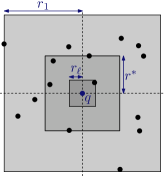
Figure 4: The considered radii $r_{i}$, and $r^{*}$, for $k=5$.

We can find the smallest radius $r_{i}$ for which $S(q,r_{i})$ contains at least $k$ points by performing binary search over the radii, performing orthogonal range counting at each step to guide the search. By performing a similar procedure for the $x$-coordinates greater than $q_{x}$, as well as for the $y$-coordinates, we obtain a set of four squares, that each contain at least $k$ points. The smallest of these squares contains exactly $k$ points and is thus $\mathcal{D}^{k}(q)$. As each procedure performs $O(\log n)$ orthogonal range counting queries, we obtain the following theorem.

Theorem 3.1.

Let $P$ be a set of $n$ points in $\mathbb{R}^{2}$. In $O(n\log n)$ time, we can build a data structure of size $O(n\log n)$, that can report $\mathcal{D}^{k}_{1}(q)$ and $\mathcal{D}^{k}_{\infty}(q)$ in $O(\log^{2}n)$ time.

Following an idea of Chan et al. [12] we can reduce the space used by replacing the binary range tree used for the orthogonal range queries by one with fanout $n^{\delta}$ for some constant $\delta>0$.

Lemma 3.2.

Let $P$ be a set of $n$ points in $\mathbb{R}^{2}$. Let $\delta>0$ be an arbitrarily small constant. In $O(n\log n)$ time, we can build a data structure of size $O(n)$, that answers orthogonal range reporting and counting queries on $P$ in $O(n^{\delta}+k^{\prime})$ time, where $k^{\prime}$ is the output size.

Proof 3.3.

Fix $\delta>0$. The data structure is a two-dimensional range tree, where the nodes in the primary tree have $\lceil n^{\delta/2}\rceil$ children, rather than $2$. This gives the primary tree a height of $O(2/\delta)$ instead of $O(\log n)$. The primary tree stores the points of $P$ sorted by $x$-coordinate. The internal nodes of the tree store balanced binary search trees as associated structures, built on the canonical subsets of the internal nodes. These binary search trees store the points sorted by $y$-coordinate.

The preprocessing time is easily seen to be $O(n\log n)$, by adapting the construction algorithm for the standard range tree to give a primary tree with higher degree. For a single level of the primary tree, the union of the canonical subsets is equal to $P$. Therefore, the associated structures in all nodes of a given level take up $O(n)$ space in total. As there are $O(2/\delta)$ levels in the primary tree, the data structure uses $O(2n/\delta)=O(n)$ space in total. The query algorithm is similar to that of a range tree. Let $Q$ be the query range, and let $Q_{\ell}$ and $Q_{r}$ be the $x$-coordinates of the left and right sides of $Q$, respectively. Then in the primary tree, we first look for the leftmost and rightmost points in $P$ whose $x$-coordinates are between $Q_{\ell}$ and $Q_{r}$. This can be done by two traversals of the primary tree, from the root to the leaves, in $O(2n^{\delta/2}/\delta)$ time total. Using these two search paths, we can now identify $O(2n^{\delta/2}/\delta)$ internal nodes, and $O(n^{\delta/2})$ leaves, such that their canonical subsets are disjoint, and together make up the set of points in $P$ whose $x$-coordinates are between $Q_{\ell}$ and $Q_{r}$. By querying the associated structures in each of these nodes, taking $O(\log n)$ time each, and combining the results, we can answer a query. The total query time is therefore $O(n^{\delta/2}\log n+k^{\prime})=O(n^{\delta}+k^{\prime})$.

Theorem 3.4.

Let $P$ be a set of $n$ points in $\mathbb{R}^{2}$. Let $\delta>0$ be an arbitrarily small constant. In $O(n\log n)$ time, we can build a data structure of $O(n)$ size, that can report $\mathcal{D}^{k}_{1}(q)$ and $\mathcal{D}^{k}_{\infty}(q)$ in $O(n^{\delta})$ time.

3.2 The $L_{2}$ metric case

In this section, we give two data structures that can report the disk $\mathcal{D}^{k}_{m}(q)$ under the $L_{2}$ metric. In Section 3.2.1, we give a solution with a randomized query time bound. Then in Section 3.2.2, we show that with a similar strategy, we can make the query time hold in the worst case. Throughout this section, we use $B$ to denote the same constant used by Agarwal et al. [3]. This is a constant depending on the number of polynomial inequalities $s$ of the ranges, the maximum degree $\Delta$ of these polynomials, and the dimension $d$. In our case. all of these are small constants.

3.2.1 Randomized $O(n^{1/2}\log^{B+1}n)$ query time

In this section, we give a simple randomized data structure that finds $\mathcal{D}^{k}(q)$ in expected $O(n^{1/2}\log^{B+1}n)$ time. The data structure consists of the large fan-out partition tree of Agarwal et al. [3], used for semialgebraic range searching. Together with this tree, we take a random sample $P^{\prime}$ of $P$ by including each point with probability $1/n^{1/2}$. Note that this random sample will contain $n^{1/2}$ points in expectation.

The main idea is to combine binary search on the ordered distances $R=\{L_{2}(q,p^{\prime})\mid p^{\prime}\in P^{\prime}\}$ with circular range counting. Let $r^{*}$ be the distance between $q$ and its $k^{th}$ nearest neighbor among $P$. We then search for two consecutive distances $r_{i},r_{i+1}\in R$, such that $r_{i}\leq r^{*}\leq r_{i+1}$. Because the number of points $p\in P$ with $r_{i}\leq L_{2}(q,p)\leq r_{i+1}$ is $n^{1/2}$ in expectation, we can then afford to report these points with semialgebraic range reporting, and combining binary search with range counting again to find $r^{*}$. This leads to an expected query time of $O(n^{1/2}\log^{B+1}n)$.

3.2.2 Worst-case $O(n^{1/2}\log^{B+1}n)$ query time

We now show how to achieve the same query time complexity as in Section 3.2.1, but in the worst case.

For now, we assume that the set $P$ lies in $D_{0}$-general position for a constant $D_{0}$ (see [3] for a definition). The details on this assumption are not important, and we will later show how to handle arbitrary point sets. The data structure consists of two copies of the large fan-out (fan-out $n^{\delta}$, for some constant $\delta>0$,) partition tree of Agarwal et al. [3], built on $P$. The first copy, which we call $\mathcal{T}$, will be augmented slightly to support generating candidate ranges (disks) that will eventually lead to $\mathcal{D}^{k}(q)$. The second copy will be used as a black box, answering circular range counting queries to guide the search for $\mathcal{D}^{k}(q)$ by counting the number of points inside the candidate ranges.

The tree $\mathcal{T}$ is constructed by recursively partitioning the space into open, connected regions, called cells. Once a cell contains a small (constant) number of points of $P$, the recursion stops and $\mathcal{T}$ gets a leaf node containing these points. There may be points of $P$ that do not lie on these cells, but rather on the zero set of the partitioning polynomial used to partition the space. For range searching with arbitrary point sets, Agarwal et al. [3] store these points in an auxiliary data structure. However, with our assumption that $P$ lies in $D_{0}$-general position, we do not need this auxiliary data structure, and will simply store the points inside a leaf node, whose parent is the node corresponding to the partitioning polynomial.

We augment $\mathcal{T}$ further as follows. We adjust $\mathcal{T}$ such that each internal node corresponding to a cell $\omega$ stores an arbitrary point in $\omega$. During the construction of $\mathcal{T}$, a point inside each cell is already computed. Hence the construction time is unaltered.

Answering a query.

To query the structure with a query point $q$, we keep track of a set of nodes $N_{i}$ for each level $i$ of $\mathcal{T}$ that is explored by our algorithm. With slight abuse of terminology, we refer to the sets $P^{\prime}$ of points stored in the leaves of $\mathcal{T}$ as cells. Let $\Omega_{i}$ denote the cells corresponding to the internal nodes in $N_{i}$, and $P_{i}$ denote the cells corresponding to the leaf nodes in $N_{i}$. We maintain the invariant that $p^{k}(q)$, the $k^{th}$ nearest neighbor of $q$, is contained in a cell in $\Omega_{i}\cup P_{i}$. Initially, $N_{1}$ contains the root node. If $\mathcal{T}$ is a single leaf, then the cell corresponding to the root node will be stored in $P_{1}$. Otherwise, it will be stored in $\Omega_{1}$.

The query algorithm works as follows. Say the algorithm is at level $i$ in $\mathcal{T}$. For a cell $\omega\in\Omega_{i}$ stored in an internal node, let $p(\omega)$ be the point inside $\omega$ that was stored with it. Let

$$R_{i}=\{L_{2}(q,p(\omega))\mid\omega\in\Omega_{i}\}\cup\bigcup_{P^{\prime}_{i}\in P_{i}}\{L_{2}(q,p)\mid p\in P^{\prime}_{i}\}$$

be the set of distances to these points $p(\omega)$, as well as to all points stored in the leaves in $P_{i}$ and in the nodes in $N_{i}$. Let $r^{*}$ be the distance between $q$ and its $k^{th}$ nearest neighbor among $P$. This is the radius of $\mathcal{D}^{k}(q)$. To find this radius, we compute the largest distance $r^{-}\in R_{i}$, and the smallest distance $r^{+}\in R_{i}$, such that $r^{-}<r^{*}\leq r^{+}$. See Figure 5.

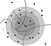
Figure 5: (left) A partitioning of $P$ into four cells. The red crosses are the points $p(\omega)$. (right) The disk $\mathcal{D}^{k}(q)$ (dashed boundary) and the disks $D(q,r^{-})$ (dotted boundary, dark gray) and $D(q,r^{+})$ (dotted boundary, light gray).

If $r^{-}$ (respectively $r^{+}$) does not exist, set it to $0$ (respectively $\infty$). We show how to compute $r^{+}$. Computing $r^{-}$ works similarly.

To compute $r^{+}$, we use a combination of median finding and binary search. For some radius $r\in R_{i}$, we decide if $r^{+}>r$ or $r^{+}\leq r$ using a circular counting query. If $D(q,r)$ contains less than $k$ points, we have $r^{+}>r$. Otherwise, we have $r^{+}\leq r$. By performing this procedure for the median radius in $R_{i}$, we can discard half of $R_{i}$ with each query.

Once we have that $r^{+}$ is the distance between $q$ and a point in $P$ (it is constructed through a leaf node of $\mathcal{T}$), we have found $r^{*}$. We then terminate the algorithm, returning the disk with the found radius. Otherwise we continue the search in the next level of $\mathcal{T}$. To continue the search through the tree, we construct the set $N_{i+1}$ by replacing every node $\nu\in N_{i}$ with its children whose cells are crossed by one of $D(q,r^{-})$ and $D(q,r^{+})$. A cell $\omega$ is crossed by a disk $D$ if $\omega\cap D\neq\emptyset$ and $\omega\nsubseteq D$. The sets $\Omega_{i+1}$ and $P_{i+1}$ are then constructed from these child nodes. Once these sets are constructed, we advance the algorithm to level $i+1$ and repeat the procedure.

We prove the correctness of the query algorithm, and bound its time complexity, in the following lemmas.

Lemma 3.5.

The query algorithm correctly returns $\mathcal{D}^{k}(q)$.

Proof 3.6.

We claim that this algorithm correctly returns $\mathcal{D}^{k}(q)$. First, note that if the algorithm returns a disk, that disk contains $k$ points, and its radius is equal to the distance between $q$ and a point of $P$. Therefore, it is indeed $\mathcal{D}^{k}(q)$. We now show that our algorithm will always return a disk, and therefore that our algorithm is correct. To show this, it suffices to show that for every level $i$ of $\mathcal{T}$ traversed by our algorithm, the set $\Omega_{i}\cup P_{i}$ contains the cell containing $p^{k}(q)$.

We give a proof by induction. It holds trivially that $\Omega_{1}\cup P_{1}$ contains a cell containing $p^{k}(q)$. We prove that if $\Omega_{i}\cup P_{i}$ contains a cell $\omega^{\prime}$ containing $p^{k}(q)$, then either the algorithm terminates and returns $\mathcal{D}^{k}(q)$, or there is a cell $\omega\in\Omega_{i+1}\cup P_{i+1}$ containing $p^{k}(q)$.

If $\omega^{\prime}\in P_{i}$, then $R_{i}$ will contain $r^{*}$. It will then find $r^{+}=r^{*}$ and terminate, returning $D(q,r^{+})=\mathcal{D}^{k}(q)$. Now assume that $\omega^{\prime}\in\Omega_{i}$. Let $\nu\in N_{i}$ be the internal node corresponding to $\omega^{\prime}$. Now let $\omega$ be the cell stored in a child of $\nu$, such that $p^{k}(q)$ lies in $\omega$. We show that $\omega\in\Omega_{i+1}\cup P_{i+1}$.

Our algorithm performs repeated median finding on the radii in $R_{i}$, resulting in the largest radius $r^{-}\in R_{i}$ and smallest radius $r^{+}\in R_{i}$, such that $D(q,r^{-})$, respectively $D(q,r^{+})$, contains less than, respectively at least, $k$ points of $P$. Let $r_{\omega}$ be the distance between $q$ and $p(\omega)$, the point in $\omega$ that was stored in $\mathcal{T}$. If $r_{\omega}<r^{*}$, then we have that $r_{\omega}\leq r^{-}$, implying that $D(q,r^{-})$ intersects $\omega$. Also, because $\omega$ is open, and because $p^{k}(q)\in\omega$, there must be a point $p^{\prime}\in\omega$ such that $r^{-}<r^{*}=L_{2}(q,p^{k}(q))<L_{2}(q,p^{\prime})$. This shows that $\omega$ is not contained in $D(q,r^{-})$, and thus that $D(q,r^{-})$ crosses $\omega$. With similar reasoning, it can be seen that if $r_{\omega}\geq r^{*}$, then $D(q,r^{+})$ crosses $\omega$. Thus, $\omega$ will be crossed by at least one of $D(q,r^{-})$ and $D(q,r^{+})$, and thus $\omega\in\Omega_{i+1}\cup P_{i+1}$. This proves the correctness of our algorithm.

Lemma 3.7.

The running time of the query algorithm is $O(n^{1/2}\log^{B+1}n)$.

Proof 3.8.

In every level of the partition tree, we perform repeated median finding on the distances stored in the sets $R_{i}$, combined with circular range counting at every step. In level $i$, the time spent performing repeated median finding is $O(|R_{i}|)$, and we perform $O(\log|R_{i}|)$ circular range counting queries. As circular range counting takes $O(n^{1/2}\log^{B}n)$ time with the partition tree [3], this brings the total time spent in level $i$ to $O(|R_{i}|+n^{1/2}\log^{B+1}|R_{i}|)$. Computing all cells $\omega$ in children of nodes in $N_{i}$ then takes $r^{c}$ time, where $r=n^{\delta}$ for a small constant $\delta>0$ is a parameter determining the fan-out of the partition tree, and $c$ is a constant. Because the partition tree has constant height, the total query time is $O(\sum_{i}|R_{i}|+n^{1/2}\log^{B+1}n+r^{c})$. By setting $\delta\leq 1/(2c)$ the query time becomes $O(\sum_{i}|R_{i}|+n^{1/2}\log^{B+1}n)$. We argue that $\sum_{i}|R_{i}|=O(n^{1/2}\log^{B}n)$.

Let $Q(n)$ be the number of nodes of $\mathcal{T}$ expanded by the query algorithm. Note that $\sum_{i}|R_{i}|=O(Q(n))$. Following the proof of Agarwal et al. [3] on the query time of the large fan-out partition tree, we assume that the number of nodes $Q(n)$ we expand satisfies $Q(n^{\prime})\leq{n^{\prime}}^{1/2}\log^{B}n^{\prime}$, for all $n_{0}<n^{\prime}<n$, where $n_{0}$ is a suitable constant determining how many points of $P$ are stored in each leaf node of $\mathcal{T}$. We now show that $Q(n)=O(n^{1/2}\log^{B}n)$.

If $n\leq n_{0}$, we have that $Q(n)=O(n)=O(1)$, and thus the bound of $Q(n)=O(n^{1/2}\log^{B}n)$ holds. We therefore assume $n>n_{0}$. Agarwal et al. [3, Lemma 4.3] proved that for any node $\nu$ of $\mathcal{T}$, and any disk $D$, the number of children of $\nu$ whose stored cell is crossed by $D$ is at most $Cr^{1/2}$, for a constant $C$ independent of $r$. The cells stored in children of $\nu$ will contain at most $n/r$ points. This means that $Q(n)$ satisfies the recurrence $Q(n)\leq Cr^{1/2}Q(n/r)$. By our assumption on a bound for $Q(n^{\prime})$, for $n^{\prime}<n$, we get that $Q(n)\leq Cr^{1/2}(n/r)^{1/2}\log^{B}(n/r)$. Since we chose $r=n^{\delta}$ for a small constant $\delta>0$, this bound simplifies to $Q(n)\leq C(1-\delta)^{B}n^{1/2}\log^{B}n=O(n^{1/2}\log^{B}n)$. The bound of $O(n^{1/2}\log^{B+1}n)$ on the query time now follows.

With the preprocessing time and space taken from Agarwal et al. [3], we obtain the following result.

Lemma 3.9.

Let $P$ be a set of $n$ points in $\mathbb{R}^{2}$, in $D_{0}$-general position for a constant $D_{0}$. Let $\delta>0$ be an arbitrarily small constant. In $O(n^{1+\delta})$ expected time, we can build a data structure of $O(n)$ size, that can report $\mathcal{D}^{k}_{2}(q)$ in $O(n^{1/2}\log^{B+1}n)$ time.

Handling arbitrary point sets.

We can lift the assumption that $P$ lies in $D_{0}$-general position by applying the perturbation scheme of Yap [44]. We refer to [3] for details, but using the perturbation scheme, $\mathcal{T}$ can be constructed on a set of points $P^{\prime}$ in $D_{0}$-general position, obtained by perturbing the individual points in $P$ by infinitesimal amounts. Clearly, using the new tree for our query algorithm can result in a disk $D$ whose radius is infinitesimally smaller or larger than that of $\mathcal{D}^{k}(q)$. In particular, the query algorithm returns the disk that has the perturbed version of $p^{k}(q)$ on its boundary. We can easily augment the data structure to return a disk with $p^{k}(q)$ itself on the boundary, rather than the perturbed version.

We augment the data structure to not only store the perturbed points in the leaves of $\mathcal{T}$, but also their original counterparts. Because our query algorithm searches for the point ${p^{\prime}}^{k}(q)$, the point $p^{k}(q)$ after perturbation, we can then augment the query algorithm to return the original point stored alongside the perturbed one. This returned point will be $p^{k}(q)$. With this point, we can then construct $\mathcal{D}^{k}(q)$. This gives us the following.

Theorem 3.10.

Let $P$ be a set of $n$ points in $\mathbb{R}^{2}$. Let $\delta>0$ be an arbitrarily small constant. In $O(n^{1+\delta})$ expected time, we can build a data structure of $O(n)$ size, that can report $\mathcal{D}^{k}_{2}(q)$ in $O(n^{1/2}\log^{B+1}n)$ time.

4 Range mode queries in two dimensions

In this section we discuss answering range mode queries in $\mathbb{R}^{2}$, and see how we can use them together with the data structures from Section 3 to answer chromatic $k\text{-NN}$ queries. In Section 4.1 we review the data structure of Chan et al. [12] that can answer range mode queries with disks (i.e. in the $L_{2}$ metric). We then show in Section 4.2 how this approach can answer range mode queries with squares (disks in the $L_{\infty}$ metric). This leads to better query times compared to directly using the existing range mode data structures for orthogonal ranges. Finally, in Section 4.3 we show that these data structures can be built efficiently, and show that this leads to efficient data structures for chromatic $k\text{-NN}$ queries.

4.1 The $L_{2}$ metric case

In this section, we present the data structure of Chan et al. [12] for finding the mode color among points in query disks. This data structure can then be used in conjunction with that of Section 3.2 to get a data structure for chromatic $k$-nearest neighbors queries.

We first transform the problem, by performing a lifting map and subsequently dualizing the points. For the lifting map, we map each point $p\in P$ to the point $\hat{p}=(p_{x},p_{y},p_{x}^{2}+p_{y}^{2})$, essentially lifting the points of $P$ to the three-dimensional unit paraboloid. Call the set of lifted points $\hat{P}$. In the following lemma, we will show that a disk $D=D(q,r)$ corresponds to the halfspace $h^{-}(q,r):z\leq 2q_{x}x+2q_{y}y-q_{x}^{2}-q_{y}^{2}+r^{2}$. See Figure 6 for an illustration of this fact.

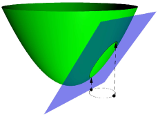
Figure 6: The lifting transformation used to transform a disk $D(q,r)$ to the halfspace $h^{-}(q,r)$.

Lemma 4.1.

Let $D=D(q,r)$ be a disk in $\mathbb{R}^{2}$. A point $p\in\mathbb{R}^{2}$ lies in $D$ if and only if $\hat{p}\in\mathbb{R}^{3}$ lies in $H(q,r)$.

Proof 4.2.

Let $p\in D$ be a point. Then we have that $(p_{x}-q_{x})^{2}+(p_{y}-q_{y})^{2}\leq r^{2}$. This implies that $p_{x}^{2}+p_{y}^{2}\leq 2q_{x}p_{x}+2q_{y}p_{y}-q_{x}^{2}-q_{y}^{2}+r^{2}$, from which it can be seen that $\hat{p}\in H(q,r)$. Following the reasoning backwards completes the proof.

Let $h^{*}$ be the point dual to the plane $h$ bounding $h^{-}(q,r)$. By taking the dual of $\hat{P}$, a set of planes $H$ is obtained, such that the points inside $D$ correspond to the planes below $h^{*}$. We will build a data structure on the set of planes $H$, that can find the mode color among these planes.

The data structure is based on the following observation by Krizanc et al. [29]:

Lemma 4.3 (Krizanc et al. [29]).

Let $A$ and $B$ be multisets. If $c$ is a mode of $A\cup B$, and $c\notin A$, then $c$ is a mode of $B$.

We apply this observation to $\frac{1}{r}$-cuttings. A $\frac{1}{r}$-cutting $\Xi$ of $\mathcal{A}(H)$ is a set of simplices with disjoint interiors, that together cover $\mathbb{R}^{3}$, such that the interior of a simplex in $\Xi$ is intersected by at most $n/r$ planes in $H$. Now let $q\in\mathbb{R}^{3}$ be a query point. Given a $\frac{1}{r}$-cutting $\Xi$ of $\mathcal{A}(H)$, let $\Delta\in\Xi$ be a simplex containing $q$, for which there is a point in $\Delta$ strictly above $q$. The mode color among the planes below $q$ is then either the color of a plane in the conflict list $H_{\Delta}$ of $\Delta$ (multiset $A$), or it is the mode color among the planes below $\Delta$ (multiset $B$). Note that Chan et al. [12] use slightly different sets. Our choice makes extending the result to the $L_{\infty}$ metric (as we do in Section 4.2) slightly easier.

The data structure.

For the data structure, we now create a $\frac{1}{r}$-cutting $\Xi$ on $H$, and for every simplex $\Delta\in\Xi$, we compute and store the mode color among the planes below $\Delta$. Aside from this cutting, we construct a point-location data structure for quickly finding the simplex containing a query point. We also need the conflict lists of the simplices. However, as they have a total size of $O(nr^{2})$, we will use a seperate data structure that computes the conflict list during a query. Lemma 4.6 states our results on cuttings and computing their conflict lists. The following lemma is used to speed up the computation of the conflict lists for our problem, where the planes of $H$ originate from two-dimensional points.

Lemma 4.4.

Let $a\in R^{3}$ be a point. We can construct, in constant time, a disk $D_{a}$ in $\mathbb{R}^{2}$, such that the points of $P$ inside $D_{a}$ correspond to those planes of $H$ below $a$.

Proof 4.5.

Let $m=(-a_{x}/2,-a_{y}/2)$ and $r=\sqrt{a_{z}-\frac{a_{x}^{2}+a_{y}^{2}}{4}}$. The disk $D_{a}=D(m,r)$ with center $m$ and radius $r$ is then lifted to the halfspace

$$h^{-}(m,r):z\leq-a_{x}-a_{y}+\frac{a_{x}^{2}+a_{y}^{2}}{4}+a_{z}-\frac{a_{x}^{2}+a_{y}^{2}}{4}=-a_{x}-a_{y}+a_{z}.$$

The plane bounding this halfspace is dual to the point $(a_{x},a_{y},a_{z})=a$. Thus, the points of $P$ inside $D_{a}$ correspond to the planes of $H$ below $a$.

Lemma 4.6.

Let $r\in[1,n]$ a parameter. We can store a $\frac{1}{r}$-cutting of $\mathcal{A}(H)$ of $O(r^{3})$ size in a data structure of $O(n+r^{3})$ size, so that the simplex $\Delta\in\Xi$ containing a query point can be found in $O(\log r)$ time, and so that reporting the conflict list of $\Delta$ takes $O(n^{1/2}\operatorname{polylog}n+n/r)$ time. Building the data structure takes expected $O(n^{1+\delta}+nr^{2})$ time.

Proof 4.7.

Using the result of Chazelle [14], we can construct, in $O(nr^{2})$ time, a $\frac{1}{r}$-cutting $\Xi$ of $O(r^{3})$ size, along with a point-location data structure, also of $O(r^{3})$ size, that answers queries in $O(\log r)$ time.

We now present a data structure for reporting the planes intersecting a simplex $\Delta$, following the ideas of Chan et al. [12]. Any plane intersecting the interior of $\Delta$ intersects the interior of an edge of $\Delta$ (without containing the edge). Beause $\Delta$ has only $O(1)$ edges, we will report the planes intersecting an edge $e$ of $\Delta$ for all edges of $\Delta$ individually. As we will then show, the number of planes reported this way will still be $O(n/r)$, even though we might report a plane multiple times.

Let $\overline{ab}$ be a line segment in $\mathbb{R}^{3}$, of which we want to report the planes intersecting it. Note that a plane intersects the interior of $\overline{ab}$ if and only if it is either strictly above $a$ and strictly below $b$, or strictly below $a$ and strictly above $b$. The first set of planes (and similarly, the second set,) can be reported using two-dimensional semialgebraic range reporting, using Lemma 4.4. Let $D_{a}$ and $D_{b}$ be the two disks in $\mathbb{R}^{2}$, such that the points inside the disks correspond to the planes below $a$ and $b$, respectively. Using the result of Agarwal et al. [3], we can construct a linear-size data structure in $O(n^{1+\delta})$ expected time, which reports the $k^{\prime}$ points strictly outside $D_{a}$ and strictly inside $D_{b}$, and thus the $k^{\prime}$ planes intersecting the interior of $\overline{ab}$, in $O(n^{1/2}\operatorname{polylog}n+k^{\prime})$ time.

Performing two of the above reporting queries per edge of $\Delta$, we obtain a query time of $O(n^{1/2}\operatorname{polylog}n+k^{\prime})$, where $k^{\prime}$ is the number of planes (including duplicates) reported in total. Note that we only report planes that intersect the interior of an edge of $\Delta$, and thus we only report planes in the conflict list of $\Delta$. Furthermore, because we perform only a constant number of reporting queries, $k^{\prime}$ will be at most a constant factor greater than the size of $H_{\Delta}$. This gives a total query time of $O(n^{1/2}\operatorname{polylog}n+n/r)$, proving the lemma.

Finally, we build a number of data structures for level queries. One is build on each set of planes in $H$ that share the same color. For these data structures, we use Lemma 4.4 to handle the queries with two-dimensional semialgebraic range counting. We use the linear-space solution of Agarwal et al. [3], which can be constructed in $O(n^{1+\delta})$ expected time and answers queries in $O(n^{1/2}\operatorname{polylog}n)$ time.

We now show how to compute the colors stored in the simplices. This can be done in $O(nr^{3})$ time, after we created pointers from each plane to a counter counting the frequency of the plane’s color. The color of a simplex can then be computed by scanning through all planes, upping a plane’s color’s frequency if the plane lies below the simplex, and keeping track of the color with the highest frequency. This takes $O(n)$ time per simplex, totalling $O(nr^{3})$ time. This brings the total size of the data structure to $O(n+r^{3})$, and the total expected preprocessing time to $O(n^{1+\delta}+nr^{3})$.

Answering a query.

Querying the structure with a point $q$ is done by first finding a simplex $\Delta\in\Xi$ containing $q$, for which there is a point in $\Delta$ strictly above $q$. This can be done in $O(\log r)$ time. Then, the conflict list of $\Delta$ is reported, taking $O(n^{1/2}\operatorname{polylog}n+n/r)$ time. Finally, for each color $c$ of the $O(n/r)$ reported planes, as well as for the color stored in $\Delta$, the number of planes below $q$ that have color $c$ is counted. Recall that this can be done using level queries. The mode color among the planes below $q$ is the color with the highest count.

Let $H_{c}$ be the set of planes with color $c$, and let $C_{\Delta}$ be the set of colors for which we perform a level query. Note that $|C_{\Delta}|=O(n/r)$. Hölders inequality now states that

$$\left(\sum_{i=1}^{m}x_{i}^{a}y_{i}^{b}\right)^{a+b}\leq\left(\sum_{i=1}^{m}x_{i}^{a+b}\right)^{a}\left(\sum_{i=1}^{m}y_{i}^{a+b}\right)^{b}$$

for any two sequences $x_{1},\dots,x_{m}$ and $y_{1},\dots,y_{m}$ and any two positive values $a$ and $b$. Applied to the level queries, we find that the level queries take a total of

$$O\left(\sum_{c\in C_{\Delta}}|H_{c}|^{1/2}\operatorname{polylog}|H_{c}|\right) =O\left(\left[\sum_{c\in C_{\Delta}}1\right]^{1/2}\left[\sum_{c\in C_{\Delta}}|H_{c}|\right]^{1/2}\operatorname{polylog}n\right)$$

$$=O((n/r^{1/2})\operatorname{polylog}n)$$

time. In total, the query time of the data structure is thus $O((n/r^{1/2})\operatorname{polylog}n)$. We thus get the following result (essentially Theorem 17 of Chan et al. [12] in the case of halfspaces in $\mathbb{R}^{3}$, though slightly improved for the case of two-dimensional circular ranges):

Proposition 4.8.

Let $P$ be a set of $n$ colored points in $\mathbb{R}^{2}$ and $r\in[1,n]$ a parameter. In $O(n^{1+\delta}+nr^{3})$ expected time, we can build a data structure of $O(n+r^{3})$ size, that reports the mode color among the points in a query disk in $O((n/r^{1/2})\operatorname{polylog}n)$ time.

4.2 The $L_{\infty}$ metric case

We can use the data structure from Section 4.2 for the problem under the $L_{\infty}$ metric as well. For a two-dimensional point $p$, the graph of its distance function

$$L_{\infty}(p,q)=\max\{|p_{x}-q_{x}|,|p_{y}-q_{y}|\}$$

forms an upside-down pyramid $\nabla_{p}$ in $\mathbb{R}^{3}$. If we now have a two-dimensional point $q$, then we have that $L_{\infty}(p,q)\leq r$ if and only if $(q_{x},q_{y},r)$ lies above $\nabla_{p}$. See Figure 7 for an illustration. Thus, by looking at the graphs of the distance functions for each point in $P$, the problem is transformed to that of finding the mode color among those graphs in $\mathbb{R}^{3}$ that lie below a given query point. We now alter the data structure of Section 4.1 to work for these graphs.

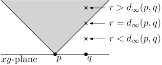
Figure 7: An illustration of the upside-down pyramid $\nabla_{p}$. The distance between $p$ and $q$ under the $L_{\infty}$ metric (in $\mathbb{R}^{2}$) determines whether the point $(q_{x},q_{y},r)$ lies strictly under, on, or strictly above $\nabla_{p}$.

The data structure.

We write $\nabla_{p}$ to denote the graph $L_{\infty}(p,\cdot)$ for a point $p\in\mathbb{R}^{2}$, and write $\nabla=\{\nabla_{p}\ |\ p\in P\}$ to be the set of graphs for all points in $P$. From now on, we will refer to the graphs as pyramids. Like for planes, we define a $\frac{1}{r}$-cutting $\Xi$ of $\mathcal{A}(\nabla)$ is a subdivision of $\mathbb{R}^{3}$ into (possibly unbounded) simplices with disjoint interiors such that the interior of each simplex is intersected by at most $n/r$ pyramids of $\nabla$. The set of pyramids intersecting the interior of a simplex $\Delta\in\Xi$ is again called the conflict list of $\Delta$. For the data structure, we need to construct a $\frac{1}{r}$-cutting for the arrangement $\mathcal{A}(\nabla)$ formed by $\nabla$, together with a point-location data structure. (See Lemma 4.6 for the case of planes.) The following lemma shows that we can use cuttings for planes to construct the desired cuttings.

Lemma 4.9.

Let $\nabla$ be a set of $n$ pyramids and $r\in[1,n]$ a parameter. In $O(nr^{2})$ time, we can construct $\frac{1}{r}$-cutting of $\mathcal{A}(\nabla)$ that consists of $O(r^{3})$ simplices. With $O(r^{3})$ additional preprocessing and space, a data structure for point location in the cutting can be build which answers queries in $O(\log r)$ time.

Proof 4.10.

Let $\nabla_{p}$ be a pyramid in $\nabla$. This pyramid is contained in the union of the four planes

$$p_{x}=x\pm z,$$

$$p_{y}=y\pm z.$$

Now let $H$ be the set of all $4n$ (not necessarily distinct) planes whose union contains all of $\nabla$. Let $\Xi$ be a $\frac{1}{4r}$-cutting of $\mathcal{A}(H)$. If the interior of a simplex $\Delta\in\Xi$ intersects a pyramid in $\nabla$, it must also intersect a plane in $H$. Therefore, the number of pyramids in $\nabla$ that intersect the interior of $\Delta$ is bounded by the number of planes in $H$ that intersect the interior of $\Delta$, which is at most $4n/(4r)=n/r$. The cutting $\Xi$ is therefore a $\frac{1}{r}$-cutting for $\mathcal{A}(\nabla)$.

If the planes of $H$ are in general position, we can use a result by Chazelle [14] to finish the proof. Unfortunately, the planes are definitely not in general position. For one, the planes constructed for a single pyramid $\nabla_{p}$ all contain $p$, meaning that four planes intersect in a single point. Moreover, for any two points $p_{1}$ and $p_{2}$, we have that the planes constructed for $\nabla_{p_{1}}$ and $\nabla_{p_{2}}$ form four pairs of parallel (or even coinciding) planes. Luckily, we can perturb the set of planes $H$ such that they do lie in general position, while keeping the properties of the constructed cutting intact [22, 21]. That is, the $\frac{1}{4r}$-cutting constructed for the perturbed planes will be a $\frac{1}{r}$-cutting for $\mathcal{A}(\nabla)$. The lemma now follow from [14].

Like for the case of planes, we need the conflict lists of the simplices. Again, however, they have a total size of $O(nr^{2})$. Hence, we use the same approach as for planes, creating an auxiliary data structure that can report the conflict list of a simplex. Note, though, that we only report a specific subset of the conflict list. This subset is still enough for the queries, and is easier to report than the entire conflict lists. The data structure is given in Lemma 4.13. We first prove the following lemma.

Lemma 4.11.

Let $p\in\mathbb{R}^{2}$ be a point. A simplex $\Delta\subset\mathbb{R}^{3}$ lies above $\nabla_{p}$ if and only if all vertices of $\Delta$ lie above $\nabla_{p}$, and any unbounded edge of $\Delta$, when seen as a ray originating from some vertex of $\Delta$, has direction $\vec{d}$, with

$$\left\{\begin{matrix}-\vec{d}_{z}\leq\vec{d}_{x}\leq\vec{d}_{z},\\ -\vec{d}_{z}\leq\vec{d}_{y}\leq\vec{d}_{z}.\end{matrix}\right.$$

Proof 4.12.

Let $p\in\mathbb{R}^{2}$ be a point and let $\Delta\subset\mathbb{R}^{3}$ be a simplex. Because $\Delta$ is a convex object, and because the area above $\nabla_{p}$ forms a convex region, we have that $\Delta$ lies above $\nabla_{p}$ if and only if all vertices and edges of $\Delta$ lie above $\nabla_{p}$. By the same argument, an edge of $\Delta$ lies above $\nabla_{p}$ if and only if its incident vertices lie above $\nabla_{p}$. This proves the theorem for bounded simplices.

Assume that $\Delta$ is unbounded, and that all vertices of $\Delta$ lie above $\nabla_{p}$. Let $e$ be an unbounded edge of $\Delta$, incident to vertex $v$. Let $\vec{d}$ be the direction of $e$, when seen as a ray originating from $v$. A point $(x,y,z)$ on $e$ now satisfies

$$\begin{cases}x=v_{x}+\lambda\vec{d}_{x}\\ y=v_{y}+\lambda\vec{d}_{y}\\ z=v_{z}+\lambda\vec{d}_{z}\end{cases}$$

for some $\lambda\geq 0$.

A point $(x,y,z)$ lies above $\nabla_{p}$ if and only if $L_{\infty}(p,(x,y))\leq z$. It follows that $e$ lies above $\nabla_{p}$ if and only if

$$\max\left\{|p_{x}-(v_{x}+\lambda\vec{d}_{x})|,|p_{y}-(v_{y}+\lambda\vec{d}_{y})|\right\}\leq v_{z}+\lambda\vec{d}_{z}$$

for all $\lambda\geq 0$, and therefore if and only if the system of equations

$$\begin{cases}v_{x}+v_{z}+\lambda(\vec{d}_{x}+\vec{d}_{z})\geq p_{x}\\ v_{x}-v_{z}+\lambda(\vec{d}_{x}-\vec{d}_{z})\leq p_{x}\\ v_{y}+v_{z}+\lambda(\vec{d}_{y}+\vec{d}_{z})\geq p_{y}\\ v_{y}-v_{z}+\lambda(\vec{d}_{y}-\vec{d}_{z})\leq p_{y}\end{cases}$$

is satisfied for all $\lambda\geq 0$. Using our assumption that all vertices of $\Delta$, and $v$ in particular, lie above $\nabla_{p}$, we now have that $e$ lies in $\nabla$ if and only if the system of equations

$$\begin{cases}\lambda(\vec{d}_{x}+\vec{d}_{z})\geq 0\\ \lambda(\vec{d}_{x}-\vec{d}_{z})\leq 0\\ \lambda(\vec{d}_{y}+\vec{d}_{z})\geq 0\\ \lambda(\vec{d}_{y}-\vec{d}_{z})\leq 0\end{cases}$$

is satisfied for all $\lambda\geq 0$. This implies that $e$ is contained in $\nabla_{p}$ if and only if $-\vec{d}_{z}\leq\vec{d}_{x}\leq\vec{d}_{z}$ and $-\vec{d}_{z}\leq\vec{d}_{y}\leq\vec{d}_{z}$.

Lemma 4.13.

Let $\delta>0$ be an arbitrarily small constant. We can store the cutting $\Xi$ in a data structure of $O(n+r^{3})$ size, so that given a simplex $\Delta\in\Xi$ and query point $q$, the subset of the conflict list of $\Delta$, containing those pyramids below $q$, can be reported in $O(n^{\delta}+n/r)$ time. Alternatively, with $O(n\log n+r^{3})$ space, the query time can be reduced to $O(\log n+n/r)$.

Proof 4.14.

Let $\Delta\subset\mathbb{R}^{3}$ be a simplex and let $q\in\Delta$ be a point. The pyramid $\nabla_{p}$ lies under $q$ if and only if $L_{\infty}(p,(q_{x},q_{y}))\leq q_{z}$. That is, $\nabla_{p}$ lies under $q$ if and only if $p\in[q_{x}-q_{z},q_{x}+q_{z}]\times[q_{y}-q_{z},q_{y}+q_{z}]=S_{q}$. See also Figure 7. Now, using Lemma 4.11, we can check in $O(1)$ time whether $\Delta$ does not lie above $\nabla_{p}$, or whether it lies above $\nabla_{p}$ if and only if the vertices of $\Delta$ lie above $\nabla_{p}$. Without loss of generality, assume that $\Delta$ lies above $\nabla_{p}$ if and only if all its vertices lie above $\nabla_{p}$, and assume that $\Delta$ is a bounded simplex.

Like for the query point $q$, a vertex $v$ of $\Delta$ lies above $\nabla_{p}$ if and only if $p$ lies in some two-dimensional axis-aligned rectangle $S_{v}$. Therefore, the points $p$ that we have to report are those in the region

$$R=S_{q}\setminus\left(\bigcap_{v\in V_{\Delta}}S_{v}\right),$$

where $V_{\Delta}$ is the set of vertices of $\Delta$. Because the intersection of two axis-aligned rectangles is an axis-aligned rectangle, the region $R$ is the difference of two axis-aligned rectangles. As there are only $O(1)$ vertices and edges in the union of the rectangles, their vertical decomposition will consist of $O(1)$ axis-aligned rectangles as well. By performing orthogonal range reporting on these rectangles, making sure not to include edges of the vertical decomposition in multiple queries, we can now report the points $p\in P$, and therefore the pyramids $\nabla_{p}$ in the conflict list of $\Delta$ that lie below $q$, using $O(1)$ orthogonal range reporting queries. Using a range tree (either using $O(n\log n)$ space [43], or $O(n)$ space with Lemma 3.2) for these queries results in the bounds in the lemma.

The final part of the data structure is the set of range counting data structures for the different sets of pyramids with equal colors. For each color $c$, let $\nabla_{c}\subset\nabla$ be the set of pyramids with color $c$. Because a point $q$ lies above a pyramid $\nabla_{p}$ if and only if $L_{\infty}(p,(q_{x},q_{y}))\leq q_{z}$, counting the number of pyramids below $q$ that have color $c$ is equivalent to counting the number of points of $P$ in the range $S((q_{x},q_{y}),q_{z})=[q_{x}-q_{z},q_{x}+q_{z}]\times[q_{y}-q_{z},q_{y}+q_{z}]$ that have color $c$. The range counting data structures therefore take the form of orthogonal range counting data structures.

Let $P_{c}\subset P$ be the set of points that have color $c$. Using a range tree, the total preprocessing time for these data structures is $O(n\log n)$. Depending on whether we use a range tree of $O(n)$ size or $O(n\log n)$ size, the total space for the range counting data structures is $O(n)$ or $O(n\log n)$, respectively.

Answering a query.

Querying the structure with a point $q$ works similarly to querying the structure of Section 4.1. First, a simplex $\Delta\in\Xi$ containing $q$ is found, for which there is a point in $\Delta$ strictly above $q$. This takes $O(\log r)$ time. Then, the pyramids in the conflict list of $\Delta$, that lie below $q$, are reported. This takes $O(Q(n)+n/r)$ time, where $Q(n)$ is the query time of the range counting data structure. Let $C_{\Delta}$ be the set of different colors of the reported pyramids. The final step is to count the frequencies of the colors in $C_{\Delta}$ among the pyramids below the query point, as well as counting the frequency of the color stored in $\Delta$. This step takes $O(n^{1+\delta}/r)$ time with a linear-sized range tree, and $O((n/r)\log n)$ time with a range tree of $O(n\log n)$ size. Thus:

Proposition 4.15.

Let $P$ be a set of $n$ points in $\mathbb{R}^{2}$. Let $r\in[1,n]$ be a parameter and $\delta>0$ an arbitrarily small constant. In $O(n\log n+nr^{3})$ time, we can build a data structure of $O(n+r^{3})$ size, that answers square range mode queries in $O(n^{1+\delta}/r)$ time. Alternatively, with $O(n\log n+r^{3})$ space, the query time can be decreased to $O((n/r)\log n)$.

4.3 Efficiently coloring cuttings

In the analyses of Sections 4.1 and 4.2, the dominating term for the preprocessing time is that of computing the colors stored in the simplices. This was done by simply scanning through the set of planes or pyramids to find the mode color among those below a given simplex, and repeating this procedure for all $O(r^{3})$ simplices. The resulting procedure takes $O(nr^{3})$ time, which, for our choice of $r$ yields a quadratic time algorithm. However, aside from this procedure, the preprocessing time is only $O(nr^{2})$. We now show how to lower the time taken to compute the colors to $O(n^{1+\delta}+n^{2/3}\cdot r^{3}+nr^{2})$ for the case of planes, and $O(n\log n+n^{\delta}\cdot r^{3}+nr^{2})$ (using $O(n)$ space) or $O(n\log n+r^{3}\log n+nr^{2})$ (using $O(n\log n)$ space) for the case of pyramids. These complexities are better than $O(nr^{3})$ for certain values of $r$, which include the values that we set $r$ to later on.

Let $S$ be a set of $n$ surfaces in $\mathbb{R}^{3}$, that are either all planes, or all upside-down pyramids. Let $\Xi$ be a $\frac{1}{r}$-cutting of $S$. The main idea behind the faster preprocessing algorithm is that we can look at the cutting $\Xi$ as a graph $G=(V,E)$, where $V$ is the set of vertices of $\Xi$ and $E$ is the set of bounded edges of $\Xi$. The algorithm traverses this graph using depth-first search, and keeps track of the frequencies of all colors among those surfaces of $S$ that lie below the current vertex. This information can then be converted into the color that we want to store in an incident simplex, using the following observation.

Let $\Delta\in\Xi$ be a simplex and let $v$ be a vertex of $\Delta$. A surface lies below $\Delta$ if and only if it lies below $v$, and it does not intersect the interior of $\Delta$.

The data structure.

For the algorithm, we use the following data structure, built on those surfaces of $S$ that lie below the current vertex. For each color $c$, we store its frequency $f_{c}$ among the surfaces in the data structure. We also keep a set of $n+1$ linked lists $L_{0},\dots,L_{n}$, such that list $L_{f}$ stores those colors whose frequency is $f$. As we want to quickly find the location of a color inside a linked list, we store pointers for each color, pointing to the element in a linked list containing the color. That is, for color $c$, we store a pointer to color $c$ in list $L_{f_{c}}$. See Figure 8 for an illustration of this part of the data structure.

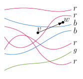
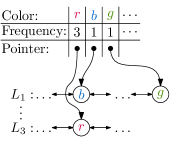
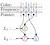
Figure 8: The data structure used during the alternative preprocessing algorithm. (left) Vertex $v$ has three red surfaces, one blue surface and one green surface below it. The algorithm moves from $v$ to $w$, crossing a red and blue surface. (middle) The status of the data structure at vertex $v$. (right) The status of the data structure at vertex $w$.

In addition, we add pointers from a surface in $S$ to its color. To keep track of the current highest frequency, we also keep the highest index $f^{*}$ for which $L_{f^{*}}$ is non-empty. This index will be used to quickly find a mode color, as every color stored in $L_{f^{*}}$ will have the highest frequency. Finally, we need a data structure that can report the surfaces in the conflict list of a simplex $\Delta\in\Xi$, which lie below a query point $q\in\Delta$. In the case where $S$ consists of planes, this data structure is that of Lemma 4.6. When $S$ consists of pyramids, this data structure is that of Lemma 4.13. Let $P(n)$ be the preprocessing time of this data structure, and let $Q(n,r)$ be its query time (both depending on the kind of surfaces that are in $S$).

During traversal of $G$, we insert and delete surfaces from the data structure. This leads to us incrementing and decrementing the frequencies of the different colors. To increment the frequency of color $c$, we first find its current frequency, which is $f_{c}$. We can then find color $c$ inside list $L_{f_{c}}$ in $O(1)$ time, by following the pointer that we stored. Removing the color from the linked list can be done in $O(1)$ time, now that we have the location of the color. Then we insert color $c$ into list $L_{f_{c}+1}$ and adjust the stored pointer to point to the new location of color $c$. This can also be done in $O(1)$ time. Finally, it might be the case that $c$ was a mode color, which would result in the frequency $f^{*}$ being incremented. To account for this, we set $f^{*}\leftarrow\max\{f^{*},f_{c}+1\}$. The whole incrementing procedure takes $O(1)$ time in total. Decrementing the frequency of a color works similarly, with the only real difference being how $f^{*}$ is updated. This is because $f^{*}$ must only be updated when $f^{*}=f_{c}$ and when $L_{f_{c}}$ is now empty. If this is the case, we simply set $f^{*}\leftarrow f_{c}-1$. As we can check whether a list is empty in $O(1)$ time, decrementing a frequency takes $O(1)$ time as well. We can therefore insert and delete surfaces from the data structure in $O(1)$ time.

The initial data structure can be built as follows. Initially, every color has frequency $0$. We therefore set every entry $f_{c}$ to $0$, add every color to list $L_{0}$, and set $f^{*}\leftarrow 0$. Say we now start the traversal at vertex $v$. Using a linear scan over $S$, we can find those surfaces that lie below $v$. Insert each of these surfaces into the data structure with the above procedure. This takes $O(n)$ time in total. The construction time of the data structure for reporting the right subsets of the conflict list of a simplex is $P(n)$, making the total initialization time $O(P(n)+n)$.

The algorithm.

We now present our algorithm. The algorithm is a depth-first search traversal through $G$, where we keep the data structure updated at every vertex. To this end, we update the data structure when traversing an edge $e=(v,w)$ by removing those surfaces that lie below $v$ and strictly above above $w$, and by inserting those surfaces that lie strictly above $v$ and below $w$. See Figure 8 for an illustration of how the data structure changes when traversing an edge. Note that all removed surfaces intersect the interior of some simplex $\Delta_{1}$, and that all inserted surfaces intersect the interior of some simplex $\Delta_{2}$, which both have $e$ as an edge. Therefore, we can report these surfaces in $O(Q(n,r))$ time. Note that we might report too many surfaces, but that the surfaces are all contained in the conflict lists of $\Delta_{1}$ and $\Delta_{2}$. For each of the reported surfaces, we can check in $O(1)$ time whether it has to be removed, inserted or ignored, after which we can update the data structure in $O(1)$ time. In total, we thus use $O(Q(n,r)+n/r)$ time to update the data structure.

When a vertex $v$ is encountered during the traversal, we assign colors to all its incident simplices, that do not have colors stored yet. If a simplex $\Delta$ does not have a color stored yet, we compute its color as follows. The current data structure contains all surfaces below $v$. By Observation 4.3, a surface below $v$ lies below $\Delta$ if and only if it does not intersect the interior of $\Delta$. Therefore, we report all surfaces that do intersect the interior of $\Delta$ (the conflict list of $\Delta$), and which lie below $v\in\Delta$, and remove these from the data structure. Finding and removing these surfaces takes $O(Q(n,r)+n/r)$ time. The result is a data structure containing precisely the surfaces below $\Delta$. Therefore, the frequency $f^{*}$ is the frequency of the color that we want to store in $\Delta$. Any color stored in list $L_{f^{*}}$ has this frequency, so we choose the head node of the list as the color to store in $\Delta$. For any vertex, we can thus compute the color to store in an incident simplex in $O(Q(n,r)+n/r)$ time in total. Afterwards, we need to undo the changes made to the data structure by reinserting the surfaces that we deleted, taking $O(Q(n,r)+n/r)$ additional time.

Combining all these components, we have a graph traversal algorithm for computing the colors stored in the simplices. The algorithm takes $O(Q(n,r)+n/r)$ time to traverse an edge. Traversing all edges therefore takes $O(Q(n,r)r^{3}+nr^{2})$ time. The total time spent computing the colors of incident vertices is $O(Q(n,r)r^{3}+nr^{2})$, as it only has to be done once per simplex. The total time spent in the vertices is therefore $O(Q(n,r)r^{3}+nr^{2})$. The result is an $O(P(n)+Q(n,r)r^{3}+nr^{2})$ time algorithm that computes the mode color among the surfaces of $S$ below a given simplex in $\Xi$, for every simplex in $\Xi$.

In the case where $S$ consists of planes, we have that $P(n)=O(n^{1+\delta})$ in expectation and $Q(n,r)=O(n^{1/2}\operatorname{polylog}n+n/r)$, by Lemma 4.6. This gives the following results.

Lemma 4.16.

Let $H$ be a set of $n$ colored planes in $\mathbb{R}^{3}$ and let $\Xi$ be a $\frac{1}{r}$-cutting of $\mathcal{A}(H)$, for some $r\in[1,n]$. We can compute the mode color among all planes in $H$ strictly below a given simplex in $\Xi$, for all simplices in $\Xi$, in $O(n^{1+\delta}+n^{1/2}r^{3}\operatorname{polylog}n+nr^{2})$ total expected time. The extra space used is $O(n)$.

Theorem 4.17.

Let $P$ be a set of $n$ colored points in $\mathbb{R}^{2}$ and $r\in[1,n]$ a parameter. In $O(n^{1+\delta}+n^{1/2}r^{3}\operatorname{polylog}n+nr^{2})$ expected time, we can build a data structure of $O(n+r^{3})$ size, that reports the mode color among the points in a query disk in $O(n^{2/3}+(n/r^{1/2})\operatorname{polylog}n)$ time.

In the case where $S$ consists of pyramids, we have that $P(n)=O(n\log n)$ and either that $Q(n,r)=O(n^{\delta}+n/r)$ (using $O(n)$ space) or $Q(n,r)=O(\log n+n/r)$ (using $O(n\log n)$ space), by Lemma 4.13. This gives the following results.

Lemma 4.18.

Let $\nabla$ be a set of $n$ colored pyramids in $\mathbb{R}^{3}$ and let $\Xi$ be a $\frac{1}{r}$-cutting of $\mathcal{A}(\nabla)$, for some $r\in[1,n]$. Let $\delta>0$ be an arbitrarily small constant. We can compute the mode color among all pyramids in $\nabla$ strictly below a given simplex in $\Xi$, for all simplices in $\Xi$, in $O(n\log n+n^{\delta}r^{3}+nr^{2})$ time total. The extra space used is $O(n)$. Alternatively, with $O(n\log n)$ extra space, the running time can be reduced to $O(n\log n+r^{3}\log n+nr^{2})$.

Theorem 4.19.

Let $P$ be a set of $n$ points in $\mathbb{R}^{2}$. Let $r\in[1,n]$ be a parameter and $\delta>0$ an arbitrarily small constant. In $O(n\log n+n^{\delta}r^{3}+nr^{2})$ time, we can build a data structure of $O(n+r^{3})$ size, that answers square range mode queries in $O(n^{1+\delta}/r)$ time. Alternatively, with $O(n\log n+r^{3})$ space, the preprocessing time can be decreased to $O(n\log n+r^{3}\log n+nr^{2})$, and the query time to $O((n/r)\log n)$.

Answering chromatic $k\text{-NN}$ queries.

In case of the $L_{2}$ distance, we use the data structure of Theorem 4.17, setting $r=n^{1/3}$ together with Theorem 3.10 to answer chromatic $k\text{-NN}$ queries. In case of the $L_{\infty}$ distance we use Theorem 4.19 with $r=n^{1/3}$ (for $O(n)$ space) or $r=(n\log n)^{1/3}$ (for $O(n\log n)$ space) together with the data structure from Theorem 3.4. We thus obtain the following results:

Theorem 4.20.

Let $P$ be a set of $n$ points in $\mathbb{R}^{2}$. There is a linear space data structure that answers chromatic $k$-NN queries on $P$ with respect to the $L_{2}$ metric. Building the data structure takes expected $O(n^{5/3})$ time, and queries take $O(n^{5/6}\operatorname{polylog}n)$ time.

Theorem 4.21.

Let $P$ be a set of $n$ points in $\mathbb{R}^{2}$. There is a linear space data structure that answers chromatic $k$-NN queries on $P$ with respect to the $L_{\infty}$ metric. Building the data structure takes $O(n^{5/3})$ worst-case time, and queries take $O(n^{2/3+\delta})$ time. We can decrease the query time to $O(n^{2/3}\log^{2/3}n)$ time using $O(n\log n)$ space and $O(n^{5/3}\log^{2/3}n)$ preprocessing time.

5 Lower bounds

We now discuss to what extent our results may be improved further. In particular, we relate the cost of chromatic $k\text{-NN}$ queries to those of range mode and range counting queries. This allows us to obtain lower bounds for chromatic $k\text{-NN}$ queries as well. We start with the following reduction.

Lemma 5.1.

Let $P$ be a set of $n$ points in $\mathbb{R}^{d}$. A range mode query with a query ball $\mathcal{D}_{m}$ (with respect to metric $m$) can be answered using a single range counting query with query range $\mathcal{D}_{m}$ and a single chromatic $k\text{-NN}$ query.

Proof 5.2.

We use the range counting query to find the number of points in the range $\mathcal{D}_{m}$. Let this be $k$, and let $q$ be the center point of the ball $\mathcal{D}_{m}$. Hence, $\mathcal{D}^{k}_{m}(q)=\mathcal{D}_{m}$, and thus the answer to the chromatic $k\text{-NN}$ query with center $q$ and value $k$ is the mode color of $\mathcal{D}_{m}$.

A conditional $\Omega(n^{1/2-\delta})$ lower bound.

We now use the above reduction to extend a conditional lower bound of Chan et al. [12] on range mode queries in arrays. They show that if in $T(n)$ time we can preprocess an array of length $n$ into a range mode data structure with query time $Q(n)$ then we can multiply two $\sqrt{n}\times\sqrt{n}$ boolean matrices in $O(T(n)+n+n\cdot Q(n))$ time. Boolean matrix multiplication of two square matrices has been researched extensively (see for example [45, 11, 23, 6]). The best combinatorial bounds merely shave off logarithmic factors from the trivial time bound, which is $O(n^{3/2})$ for two $\sqrt{n}\times\sqrt{n}$ matrices. Hence, this shows strong evidence that the query time for range mode queries must either have a worst-case preprocessing time that is $\omega(n^{3/2-\delta})$, or a worst-case query time that is $\omega(n^{1/2-\delta})$, assuming only combinatorial techniques may be used. As we argue next, the same holds for the query time of chromatic $k\text{-NN}$ queries of $n$ points in $\mathbb{R}^{1}$ in a $L_{m}$-metric.

Consider an array $A$. We map each entry $A[i]$ to the point $p_{i}=i$ in $\mathbb{R}^{1}$, and assign this point color $A[i]$. A query now asks for the mode element inside a subarray $A[\ell\mathrel{:}r]$. We answer this query using the approach in Lemma 5.1. That is, we take query range $\mathcal{D}=[p_{\ell},p_{r}]$, which is a disk in $\mathbb{R}^{1}$, and can be computed in constant time from the query pair $\ell,r$. Furthermore, since we know $\ell$ and $r$ we can answer the range counting query on $\mathcal{D}$ in constant time by simply reporting $k=r-\ell+1$. By Lemma 5.1 it thus follows that if answering the $k\text{-NN}$ query takes $O(Q(n))$ time and uses $S(n)$ space, so does answering the range mode query. This implies the following result (following Chan et al. [12]).

Theorem 5.3.

Assume that in $T(n)$ time, we can build a data structure that answers chromatic $k$-nearest neighbors queries on a set of $n$ points in $\mathbb{R}^{1}$ under any $L_{m}$ metric in $Q(n)$ time. We can then perform boolean matrix multiplication of two $\sqrt{n}\times\sqrt{n}$ matrices in $O(T(n)+n+n\cdot Q(n))$ time.

Theorem 5.3 thus shows strong evidence that using near-linear space and preprocessing time chromatic $k\text{-NN}$ queries require $\Omega(n^{1/2-\delta})$ time.

Relations to range counting queries.

Next, we relate the cost of range finding queries, i.e. the problem solved in our first step, to range counting queries. Given a data structure for range finding queries we can answer range counting queries using only logarithmic overhead:

Lemma 5.4.

Let $P$ be a set of $n$ points in $\mathbb{R}^{d}$. A range counting query on $P$ with a disk $\mathcal{D}_{m}$ under metric $m$ can be performed using $O(\log n)$ range finding queries.

Proof 5.5.

Let $q$ be the center of the query disk. We binary search over the integers $0,\dots,n$, using a range finding query to find a disk $\mathcal{D}^{k}_{m}(q)$ for each considered integer $k$. If the reported disk is smaller than $\mathcal{D}_{m}$, the number of points inside $\mathcal{D}_{m}$ is at least $k$. Otherwise, the number of points is smaller than $k$. It follows that with $O(\log n)$ range finding queries, we can count the number of points in $\mathcal{D}_{m}$.

It thus follows that range finding is roughly as difficult as range counting. In particular, a $Q(n)$ time lower bound for range counting queries using $S(n)$ space implies an $\tilde{\Omega}(Q(n))$ time lower bound for range finding queries with $S(n)$ space. For example, in the semigroup model there is an $\tilde{\Omega}(n/S(n)^{1/d})$ time lower bound for halfspace range counting [5]. Since every halfspace is a disk $\mathcal{D}_{2}$ (of radius $\infty$), this lower bound also holds for range counting with disks in the $L_{2}$ metric, and thus also for range finding.

The range mode queries from step 2 are also related to a form of range counting. A “type-2” range counting query with query range $Q$ asks for all the distinct colors appearing in $Q$ together with their frequencies, i.e. for each reported color $c$ we must also report the number of points in $P\cap Q$ that have color $c$ [13]. Clearly, answering “type-2” queries is more difficult than range counting (just assign all points the same color), so the above lower bounds also hold for “type-2” queries. Such “type-2” queries however also allow us to solve the range mode problem. When the number of colors is small (e.g. two), and we already know the number of points $k$ in the query range $\mathcal{D}^{k}(q)$ it seems that answering range mode queries is not much easier than answering (“type-2”) range counting queries. We therefore conjecture that answering range mode queries is roughly as difficult as answering range counting queries.

Conjecture 5.6.

If answering a range counting query with a query range $\mathcal{D}$ using $S(n)$ space requires $Q(n)$ time then answering a range mode query with query range $\mathcal{D}$ using $S(n)$ space requires $\tilde{\Omega}(Q(n))$ time.

Note that this conjecture together with Lemma 5.1 would imply that answering a $k\text{-NN}$ query is at least as hard as answering a range counting query. Furthermore, since we can answer a range counting query using $O(\log n)$ range finding queries (Lemma 5.4) that would then mean our two-step approach has negligible overhead with respect to an optimal solution to chromatic $k\text{-NN}$ queries.

6 The approximate problems

In this section we consider $\varepsilon$-approximate chromatic $k\text{-NN}$ queries. Our goal is to report a color $c$ that occurs at least $(1-\varepsilon)f^{*}$ times, where $f^{*}$ is the frequency of the mode color $c^{*}$ of $k\text{-NN}(q)$. We again use the two-step approach of finding the range $\mathcal{D}^{k}(q)$ (step (1)) and computing the mode of the range (step (2)). We use exact range finding data structures, and focus our attention on approximating step (2) for two reasons: first, the running times in our exact solutions are dominated by step (2), and second, it is unclear how to use approximate solutions to $k\text{-NN}$ queries (that is, approximate ranges) and still obtain guarantees on the approximation factor of our $\varepsilon$-approximate chromatic $k\text{-NN}$ queries.

For points in $\mathbb{R}^{1}$ we can again compute $\mathcal{D}^{k}(q)$ exactly using the Theorem 2.2 data structure, and then directly use the $O(n/\varepsilon)$ space data structure by Bose et al. [9] to answer the remaining $(1-\varepsilon)$-approximate range mode query. We thus get:

Theorem 6.1.

Let $P$ be a set of $n$ points in $\mathbb{R}$ and $\varepsilon\in(0,1)$ a parameter. In $O(n\log_{\frac{1}{1-\varepsilon}}n)$ time, we can build a data structure of $O(n/\varepsilon)$ size, that answers approximate chromatic $k\text{-NN}$ queries on $P$ under any $L_{m}$ metric, with $m\geq 1$, in $O(\log n+\log\log_{\frac{1}{1-\varepsilon}}n)$ time.

We now focus on the problem for points in $\mathbb{R}^{2}$. We can again use our data structures from Section 3 to efficiently find the range $\mathcal{D}^{k}(q)$ containing $k\text{-NN}(q)$. In Section 6.1 we now show that we can answer $\varepsilon$-approximate range queries with disks in roughly $\tilde{O}(n^{1/2}\varepsilon^{-3/2})$ time (ignoring polylogarithmic factors), while still using near linear space. In Section 6.2 we extend this approach to the $L_{\infty}$ metric.

6.1 Approximate chromatic $k\text{-NN}$ queries under the $L_{2}$ metric

We develop a data structure storing $P$ that can efficiently answer $\varepsilon$-approximate range mode queries with a query disk $Q$ of radius $r$. To this end, we again transform $P$ into a set of planes $H$ like in Section 4.1. The query disk now corresponds to a vertical halfline with top endpoint $h^{*}$, the point dual to the plane $h:z=2q_{x}x+2q_{y}y-q_{x}^{2}-q_{y}^{2}+r^{2}$. So, the mode color $c^{*}$ of $P\cap Q$ is the most frequently occurring color among the planes passing below $h^{*}$, and our aim is to report a color $c$ such that at least $(1-\varepsilon)f^{*}$ planes of that color pass below $h^{*}$.

The $k$-level of the arrangement $\mathcal{A}(H)$ of planes is the set of points that lie on a plane in $H$ and which have exactly $k$ planes passing strictly below them. An $\varepsilon$-approximate $k$-level of $\mathcal{A}(H)$ is a piecewise linear triangulated terrain, so every vertical line intersects it once, that lies in between the $k$-level and $(1+\varepsilon)k$-level of $\mathcal{A}(H)$. Har-Peled et al. [25] show that such an $\varepsilon$-approximate $k$-level exists, has complexity $O\left(\frac{n}{\varepsilon^{3}k}\right)$, and can be computed in $O(n(\frac{1}{\varepsilon^{3}}+\frac{1}{k\varepsilon^{6}}\log^{3}\frac{n}{k}+\log\frac{n}{k\varepsilon}))$ expected time.

The main idea to answer approximate range mode queries efficiently is to compute, for each color $c$, a series of $g(\varepsilon)$-approximate $k_{i}$-levels (for some function $g$) considering only the planes of color $c$. For each choice of $i$, we then consider the lower envelope $\mathcal{L}_{i}$ of all those $k_{i}$-levels among the various colors. See Figure 9 for an illustration. Now observe that if $h^{*}$ lies in between $\mathcal{L}_{i}$ and $\mathcal{L}_{i+1}$, the frequency $f^{*}$ of a mode color $c^{*}$ may only be a $g(\varepsilon)$ fraction larger than $k_{i+1}$, while the frequency of the color defining $\mathcal{L}_{i}$ directly below $h^{*}$ is at least $k_{i}$. So if $g(\varepsilon)$ and $k_{i}/k_{i+1}$ are sufficiently small this is a $(1-\varepsilon)$-approximation. One additional complication is that even though our $g(\varepsilon)$-approximate $k_{i}$-levels have fairly small complexity, their lower envelopes do not. So, we need to design a data structure that can test if $h^{*}$ lies above or below $\mathcal{L}_{i}$ without explicitly storing $\mathcal{L}_{i}$. We show that with near-linear space we can answer such queries in $O_{\varepsilon}(n^{1/2})$ time.

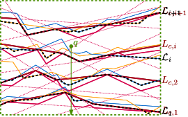
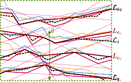
Figure 9: (left) An illustration of the idea in $\mathbb{R}^{2}$, the planes (here lines) of a single color, their $k_{i}=\left(\frac{1}{1-\alpha}\right)^{i}$-levels (bright red), and the $g(\varepsilon)$-approximate $k_{i}$-levels $L_{c,0},L_{c,1},\dots$ (in dark red). (right) For each $i$, the $\mathcal{L}_{i}$ forms the lower envelope of the $L_{c,i}$ surfaces over all colors $c$. We search for the largest $i$ for which $q$ lies above $\mathcal{L}_{i}$ (dashed).

Set $\alpha=1-\sqrt{1-\varepsilon}$, and let $H_{c}$ be the set of planes in $H$ with color $c$. For each set $H_{c}$, we consider the $\frac{\alpha}{1-\alpha}$-approximate $\left(\frac{1}{1-\alpha}\right)^{i}$-levels $L_{c,i}$ of $\mathcal{A}(H_{c})$, for $i=0,\dots,\log_{\frac{1}{1-\alpha}}|H_{c}|$, and we define $\mathcal{L}_{i}$ to be the lower envelope (the $0$-level) of the (arrangement of the) surfaces $\mathcal{L}_{c,i}$ over all colors $c$. Hence we have $k_{i}=\left(\frac{1}{1-\alpha}\right)^{i}$, and $g(\varepsilon)=\frac{1-\sqrt{1-\varepsilon}}{\sqrt{1-\varepsilon}}$. For any point $p$, let $\mathcal{L}_{i}(p)$ be the point of intersection between $\mathcal{L}_{i}$ and the vertical line through $p$. The following lemma now states that we can use these approximate levels to find an approximate mode color.

Lemma 6.2.

For any $\alpha>0$ and any positive integer $i$, the surface $\mathcal{L}_{i+1}$ lies above $\mathcal{L}_{i}$.

Proof 6.3.

For any color $c$, the surface $L_{c,i}$ lies below the

$$\left(1+\frac{\alpha}{1-\alpha}\right)\left(\frac{1}{1-\alpha}\right)^{i}=\left(\frac{1-\alpha}{1-\alpha}+\frac{\alpha}{1-\alpha}\right)\left(\frac{1}{1-\alpha}\right)^{i}=\frac{1}{1-\alpha}\left(\frac{1}{1-\alpha}\right)^{i}=\left(\frac{1}{1-\alpha}\right)^{i+1}$$

level of $\mathcal{A}(H_{c})$. Since $L_{c,i+1}$ is an approximate $\left(\frac{1}{1-\alpha}\right)^{i+1}$-level, it thus follows that $L_{c,i}$ lies below $L_{c,i+1}$. Since this holds for any color, it also holds for $\mathcal{L}_{i}$ and $\mathcal{L}_{i+1}$: for any point $p$ on $\mathcal{L}_{i+1}$, let $L_{c,i+1}$ be the surface realizing $\mathcal{L}_{i+1}$ at $p$. By the above argument it then follows that $L_{c,i}(p)$ lies below $\mathcal{L}_{i+1}(p)$, and hence $\mathcal{L}_{i}$ also lies below $\mathcal{L}_{i+1}(p)$.

Lemma 6.4.

Let $q\in\mathbb{R}^{3}$ be a point, let $f^{*}$ be the exact frequency of the mode color among the planes below $q$, and let $i$ be the largest integer for which $q$ lies above $\mathcal{L}_{i}$. Any color $c$ for which $q$ lies above $L_{c,i}$ occurs at least $(1-\varepsilon)f^{*}$ times among the planes below $q$.

Proof 6.5.

Because $i$ is the largest integer for which $q$ lies above $\mathcal{L}_{i}$ it follows that, for any color $c$, the point $q$ lies strictly below $L_{c,i+1}$ (otherwise it would also have been above $\mathcal{L}_{i+1}$). This holds in particular for the mode color $c^{*}$. Since $q$ lies below $L_{c^{*},i+1}$, it lies strictly below the $\left(\frac{1}{1-\alpha}\right)^{i+2}$-level of $\mathcal{A}(H_{c^{*}})$. We obtain $\displaystyle f^{*}<\left(\frac{1}{1-\alpha}\right)^{i+2}+1=\left(\frac{1}{1-\varepsilon}\right)^{i/2+1}+1$ and thus

$$(1-\varepsilon)f^{*}<\left(\frac{1}{1-\varepsilon}\right)^{i/2}+(1-\varepsilon).$$ (1)

For any color $c$ for which $q$ lies above $L_{c,i}$ we have that $q$ lies above the $\left(\frac{1}{1-\alpha}\right)^{i}$-level of $\mathcal{A}(H_{c})$. We thus get the following lower bound for the number of planes of color $c$ below $q$:

$$\left(\frac{1}{1-\alpha}\right)^{i}+1=\left(\frac{1}{1-\varepsilon}\right)^{i/2}+1\leq f_{c}.$$ (2)

Combining equations 1 and 2 we obtain that for a color $c$ for which $q$ lies above $L_{c,i}$ we have

$$(1-\varepsilon)f^{*}<\left(\frac{1}{1-\varepsilon}\right)^{i/2}+(1-\varepsilon)<\left(\frac{1}{1-\varepsilon}\right)^{i/2}+1\leq f_{c}.$$

Hence, $f_{c}\geq(1-\varepsilon)f^{*}$. Note that there is at least one color $c$ for which $q$ lies above $L_{c,i}$, and thus for which $f_{c}\geq(1-\varepsilon)f^{*}$, namely the color defining $\mathcal{L}_{i}$ at $\mathcal{L}_{i}(h^{*})$.

By Lemma 6.4 we can answer an $\varepsilon$-approximate range mode color query by finding the largest integer $i$ among $0,\dots,\log_{\frac{1}{1-\alpha}}n$ for which $h^{*}$ lies above $\mathcal{L}_{i}$. By Lemma 6.2, all $\mathcal{L}_{0}(h^{*}),\mathcal{L}_{1}(h^{*}),\dots$ are monotonically increasing. Hence, we can find $i$ using a binary search. Note that if $h^{*}$ lies below $\mathcal{L}_{0}$, every color will have a frequency of at most one. We can answer an exact chromatic $k\text{-NN}$ query in this case with range reporting, reporting the color of an arbitrary point in the range. This step does not affect the asymptotic complexities.

Now assume that $h^{*}$ lies above $\mathcal{L}_{0}$. To find the largest integer $i$ for which $h^{*}$ lies above $\mathcal{L}_{i}$, we need to be able to compute a points $\mathcal{L}_{j}(h^{*})$ (for some given $j$). We now argue that we can do this efficiently while using only near linear space.

Computing $\mathcal{L}_{j}(h^{*})$.

One solution would be to explicitly compute the lower envelope of (the triangles making up) the $L_{i,c}$ surfaces, over all colors $c$. However, this envelope may have quadratic size [20, 39]. We will therefore use a ray shooting based approach instead [2, 18].

Lemma 6.6.

Let $\mathcal{T}$ be a set of $m$, possibly intersecting, possibly unbounded, triangles in $\mathbb{R}^{3}$. In $O(m\log^{4}m)$ time, we can build a data structure of size $O(m\log^{2}m\log\log m)$ that can report the lowest triangle in $\mathcal{T}$ along a vertical line $\ell_{q}$ in $O(m^{1/2}\log^{2}m)$ expected time.

Proof 6.7.

The main idea is to project the triangles onto the horizontal plane $z=0$, and store this set $\bar{\mathcal{T}}$ of projected triangles in a data structure for stabbing queries. In particular, a data structure that can return the triangles stabbed by a query point $q$ as few ($O(m^{1/2}\log^{2}m)$) canonical subsets $\bar{\mathcal{T}^{\prime}}$, i.e. fixed subsets of triangles stored in the data structure. On the domain where the $q$ stabs all triangles in such a canonical subset $\bar{\mathcal{T}^{\prime}}$ we can treat their original triangles $\mathcal{T}^{\prime}$ as planes. Hence, using linear space we can store the lower envelope of these planes so that we can efficiently (i.e. in $O(\log|\bar{\mathcal{T}^{\prime}}|)$ time) report the lowest plane (and thus triangle) of $\bar{\mathcal{T}^{\prime}}$ intersected by $\ell_{q}$. We then report the lowest triangle intersected over all canonical subsets. Next, we describe the implementation of our data structure in more detail.

Every projected triangle $\bar{\Delta}$ is the intersection of (at most) three halfplanes $h_{1}$,$h_{2}$, and $h_{3}$. We dualize the lines bounding these halfplanes into three points $p_{1}(\bar{\Delta})$, $p_{2}(\bar{\Delta})$, and $p_{3}(\bar{\Delta})$, respectively, and the query point $q$ into a line $\rho$. The query point $q$ lies in $h_{1}$ if and only if $\rho$ passes $p_{1}(\bar{\Delta})$ on the side corresponding to $h_{1}$. It thus follows that $q$ lies in the triangle $\bar{\Delta}$ if and only if $\rho$ passes $p_{1}(\bar{\Delta})$, $p_{2}(\bar{\Delta})$, and $p_{3}(\bar{\Delta})$ on the appropriate sides. We build a three-level partition tree on these points [10]. In particular, the first level is a partition tree on the $p_{1}(\bar{\Delta})$ points over all over all triangles $\Delta\in T$. Each internal node $\nu$ corresponds to a subset of the points, and thus a subset $\mathcal{T}_{\nu}$ of triangles, (namely the points stored in the leaves of the subtree) and stores a partition tree on the $p_{2}(\bar{\Delta})$ points of a triangle $\Delta\in\mathcal{T}_{\nu}$. In turn, the internal nodes of this tree store one more partition tree on the $p_{3}$ points. Each node $\mu$ in a third level partition tree corresponds to some region $R_{\mu}$ of the (primal) plane (at $z=0$) that is contained in all of the (projections of the) triangles of its associated set $T_{\mu}$. Hence, $\mu$ stores the lower envelope of the supporting planes of the triangles in $\mathcal{T}_{\mu}$ preprocessed for $O(\log|\mathcal{T}_{\mu}|)$ time vertical ray shooting queries. Since this lower envelope has linear complexity, such a data structure (essentially a point location data structure) uses only linear space [41]. We apply Corollary 7.2(i) of Chan [10] for the trees in the first two levels, and then Corollary 7.2(ii) for the third level trees. It then follows that the total space used is $O(m\log^{2}m\log\log m)$, and that the data structure can be built in $O(m\log^{4}m)$ time. For a query $q$, we can select (in expectation) $O(m^{1/2}\log^{2}m)$ nodes $\mu$ of the third level trees whose canonical subsets $\mathcal{T}_{\mu}$ make up exactly the triangles stabbed by $q$ [10]. For each such a node $\mu$ we thus have $q\in R_{\mu}$, and hence we can find the lowest triangle vertically above $q$ by querying the lower envelope of the planes in $O(\log|\mathcal{T}_{\mu}|)$ time. As the canonical subsets can be selected in $O(m^{1/2}\log^{2}m)$ expected time, and have the property that $\sum_{\mu}\log\mathcal{T}_{\mu}=O(m^{1/2}\log^{2}m)$, it follows that the total expected query time is $O(m^{1/2}\log^{2}m)$.

Remark 6.8.

Chan remarks that the above bound can likely be made to hold w.h.p. (i.e. probability $1-\frac{1}{m^{c_{0}}}$, for an arbitrarily large constant $c_{0}$) [10]. If we require worst case query time, we can also use the partition tree by Matoušek [35]. This increases the preprocessing time to $O(m^{1+\delta})$, the space to $O(n\operatorname{polylog}n)$ and the query time to $O(m^{1/2}\operatorname{polylog}m)$, for some arbitrarily small $\delta>0$.

Analysis.

We now analyze the space usage and the preprocessing and query time.

Lemma 6.9.

The total complexity of the approximate levels is $O(n/\alpha^{4})$, and they can be computed in $O\left(n\left(\frac{\log_{\frac{1}{1-\alpha}}n}{\alpha^{3}}+\frac{\log^{3}n}{\alpha^{7}}+\log\left(\frac{n}{\alpha}\right)\log_{\frac{1}{1-\alpha}}n\right)\right)$ expected time.

Proof 6.10.

Let $A$ be a sufficiently large constant. The total complexity of the approximate levels is then

$$\sum_{c}\sum_{i=0}^{\log_{\frac{1}{1-\alpha}}|H_{c}|}\frac{A\cdot|H_{c}|}{\left(\frac{\alpha}{1-\alpha}\right)^{3}\cdot\left(\frac{1}{1-\alpha}\right)^{i}} =A\sum_{c}\sum_{i=0}^{\log_{\frac{1}{1-\alpha}}|H_{c}|}\frac{|H_{c}|}{\frac{\alpha^{3}}{(1-\alpha)^{3}}\cdot\left(\frac{1}{1-\alpha}\right)^{i}}$$

$$=A\sum_{c}\frac{|H_{c}|}{\alpha^{3}}\sum_{i=0}^{\log_{\frac{1}{1-\alpha}}|H_{c}|}\frac{1}{\frac{1}{(1-\alpha)^{3}}\cdot\frac{1}{(1-\alpha)^{i}}}$$

$$\leq A\frac{n}{\alpha^{3}}\sum_{i=0}^{\log_{\frac{1}{1-\alpha}}n}\frac{1}{\frac{1}{(1-\alpha)^{i+3}}}$$

$$=A\frac{n}{\alpha^{3}}\sum_{i=0}^{\log_{\frac{1}{1-\alpha}}n}(1-\alpha)^{i+3}.$$

Using that $\sum_{i=0}^{\infty}(1-\alpha)^{i}$ is a geometric series that converges to $1/(1-(1-\alpha))=1/\alpha$ it then follows that the total complexity of the approximate levels is $O(n/\alpha^{4})$.

Recall that an $\varepsilon$-approximate $k$-level can be computed in $O(n(\frac{1}{\varepsilon^{3}}+\frac{1}{k\varepsilon^{6}}\log^{3}\frac{n}{k}+\log\frac{n}{k\varepsilon}))=O(n(\frac{1}{\varepsilon^{3}}+\frac{1}{k\varepsilon^{6}}\log^{3}n+\log\frac{n}{\varepsilon}))$ expected time [25]. The total time to construct our approximate levels is then

$$\sum_{c}\sum_{i=0}^{\log_{\frac{1}{1-\alpha}}|H_{c}|}O\left(|H_{c}|\left(\frac{1}{\left(\frac{\alpha}{1-\alpha}\right)^{3}}+\frac{1}{\left(\frac{1}{1-\alpha}\right)^{i}\left(\frac{\alpha}{1-\alpha}\right)^{6}}\log^{3}|H_{c}|+\log\left(\frac{|H_{c}|}{\frac{\alpha}{1-\alpha}}\right)\right)\right)$$

$$=O\left(\sum_{c}|H_{c}|\sum_{i=0}^{\log_{\frac{1}{1-\alpha}}n}\left(\frac{1}{\frac{\alpha^{3}}{(1-\alpha)^{3}}}+\frac{1}{\frac{\alpha^{6}}{(1-\alpha)^{i+6}}}\log^{3}n+\log\left(\frac{n(1-\alpha)}{\alpha}\right)\right)\right)$$

$$=O\left(n\sum_{i=0}^{\log_{\frac{1}{1-\alpha}}n}\left(\frac{(1-\alpha)^{3}}{\alpha^{3}}+\frac{(1-\alpha)^{i+6}}{\alpha^{6}}\log^{3}n+\log\left(\frac{n}{\alpha}\right)\right)\right)$$

$$=O\left(n\left(\sum_{i=0}^{\log_{\frac{1}{1-\alpha}}n}\frac{(1-\alpha)^{3}}{\alpha^{3}}+\sum_{i=0}^{\log_{\frac{1}{1-\alpha}}n}\frac{(1-\alpha)^{i+6}}{\alpha^{6}}\log^{3}n+\sum_{i=0}^{\log_{\frac{1}{1-\alpha}}n}\log\left(\frac{n}{\alpha}\right)\right)\right)$$

$$=O\left(n\left(\frac{\log_{\frac{1}{1-\alpha}}n}{\alpha^{3}}+\frac{\log^{3}n}{\alpha^{7}}+\log\left(\frac{n}{\alpha}\right)\log_{\frac{1}{1-\alpha}}n\right)\right).$$

It now follows from Lemma 6.9 that the ray-shooting data structures from Lemma 6.6 have total size $O(\frac{n}{\alpha^{4}}\log^{2}\left(\frac{n}{\alpha^{4}}\right)\log\log\left(\frac{n}{\alpha^{4}}\right))$, and that they can be built in expected $O(\frac{n}{\alpha^{4}}\log^{4}\left(\frac{n}{\alpha^{4}}\right))$ time. The ray shooting data structure on $\mathcal{L}_{i}$ is built on at most

$$O\left(\sum_{c}\frac{|H_{c}|}{\left(\frac{\alpha}{1-\alpha}\right)^{3}k_{i}}\right)=O\left(\frac{n}{\left(\frac{\alpha}{1-\alpha}\right)^{3}}\right)=O(n/\alpha^{3})$$

triangles. It then follows that the expected time to answer a chromatic range mode query is $O\left(\frac{n^{1/2}}{\alpha^{3/2}}\log^{2}\frac{n}{\alpha}\log\log_{\frac{1}{1-\alpha}}n\right)$. Using that $\varepsilon/2\leq\alpha=1-\sqrt{1-\varepsilon}\leq\varepsilon$ we then also obtain the following result.

Theorem 6.11.

Let $P\subset\mathbb{R}^{2}$ be a set of $n$ points and let $\varepsilon\in(0,1)$. In expected

$$O\left(n\left(\frac{\log_{\frac{1}{1-\varepsilon}}n}{\varepsilon^{3}}+\frac{\log^{3}n}{\varepsilon^{7}}+\log\left(\frac{n}{\varepsilon}\right)\log_{\frac{1}{1-\varepsilon}}n+\frac{\log^{4}\frac{n}{\varepsilon}}{\varepsilon^{4}}\right)\right)\quad\mathit{time,}$$

we can build a $O\left(\frac{n}{\varepsilon^{4}}\log^{2}\frac{n}{\varepsilon}\log\log\frac{n}{\varepsilon}\right)$ size data structure that answers $\varepsilon$-approximate chromatic range mode queries disks in expected $O\left(\frac{n^{1/2}}{\varepsilon^{3/2}}\log^{2}\frac{n}{\varepsilon}\log\log_{\frac{1}{1-\varepsilon}}n\right)$ time.

Answering $\varepsilon$-approximate chromatic $k\text{-NN}$ queries.

Since we can find the smallest disk $\mathcal{D}^{k}(q)$ containing $k\text{-NN}(q)$, and thus the point dual to $\mathcal{D}^{k}(q)$, in $O(n^{1/2}\operatorname{polylog}n)$ time using Theorem 3.10, we can then also answer $\varepsilon$-approximate chromatic $k\text{-NN}$ queries:

Theorem 6.12.

Let $P\subset\mathbb{R}^{3}$ be a set of $n$ points and let $\varepsilon\in(0,1)$. In expected

$$O\left(n^{1+\delta}+n\left(\frac{\log_{\frac{1}{1-\varepsilon}}n}{\varepsilon^{3}}+\frac{\log^{3}n}{\varepsilon^{7}}+\log\left(\frac{n}{\varepsilon}\right)\log_{\frac{1}{1-\varepsilon}}n+\frac{\log^{4}\frac{n}{\varepsilon}}{\varepsilon^{4}}\right)\right)\quad\mathit{time,}$$

we can build a $O\left(\frac{n}{\varepsilon^{4}}\log^{2}\frac{n}{\varepsilon}\log\log\frac{n}{\varepsilon}\right)$ size data structure that answers $\varepsilon$-approximate chromatic $k\text{-NN}$ queries on $P$ under the $L_{2}$ metric in expected

$$O\left(n^{1/2}\operatorname{polylog}n+\frac{n^{1/2}}{\varepsilon^{3/2}}\log^{2}\frac{n}{\varepsilon}\log\log_{\frac{1}{1-\varepsilon}}n\right)\quad\mathit{time.}$$

6.2 Approximate chromatic $k\text{-NN}$ queries under the $L_{\infty}$ metric

In this section we show that the data structure from Section 6.1 can be adapted to answer $\varepsilon$-approximate range mode queries with axis aligned squares. Therefore, we can also efficiently answer $\varepsilon$-approximate chromatic $k\text{-NN}$ queries in the $L_{\infty}$ metric. The main idea remains the same as before: (i) we transform the points into surfaces in $\mathbb{R}^{3}$ and the query range $Q$ into a vertical downward half-line, (ii) we compute a series of $g(\varepsilon)$-approximate $k_{i}$-levels on the surfaces of each color, and (iii) for each $i$ we store the lower envelope $\mathcal{L}_{i}$ of those approximate levels over all colors. Via the same argument as before it then follows that if the top endpoint of the vertical half-line lies in between $\mathcal{L}_{i}$ and $\mathcal{L}_{i+1}$, the color realizing $\mathcal{L}_{i}$ is an answer to the $\varepsilon$-approximate range mode query.

Recall from Section 4.2 that (i) we can map each point $p\in P$ to the graph of $L_{\infty}(p,\cdot)$, which we refer to as a pyramid, and that (ii) an axis parallel query square $Q$ of radius $r$ then corresponds to the vertical halfline with topmost point $\hat{q}=(q_{x},q_{y},r)$. Let $\nabla$ denote the set of all such pyramids. As in the case for planes these pyramids define an arrangement $\mathcal{A}(\nabla)$, and an ($\varepsilon$-approximate) $k$-level in this arrangement. Since the $L_{\infty}$-Voronoi diagram on $P$ has linear complexity [31], so does the $0$-level of $\mathcal{A}(\nabla)$. Kaplan et al. [27] then show that an $\varepsilon$-approximate $k$-level has complexity $O(\frac{n}{\varepsilon^{5}k}\log^{2}n)$. Moreover, they show how to construct an $\frac{1}{2}$-approximate $k$-level in $O(n\lambda_{s}(\log n)\log^{2}n)$ time, where $\lambda_{s}(m)$ denotes the maximum length of a Davenport-Schinzel sequence of order $s$ on $m$ symbols. The value of $s$ depends on the type of surfaces under consideration (refer to Kaplan et al. [27] for details). In our case, we have $s=4$ (see [27, Section 9]), and hence $\lambda_{4}(m)$ is near linear in $m$. Next, we argue that we can also use the algorithm of Kaplan et al.to compute $\varepsilon$-approximate levels for different values $\varepsilon>0$.

Lemma 6.13.

Let $\nabla$ be a set of $n$ pyramids. Let $1\leq k\leq n$ and let $\varepsilon\in(0,1/2]$. In $O\left(\frac{n}{\varepsilon^{2}}\lambda_{4}\left(\frac{\log n}{\varepsilon^{2}}\right)\log^{3}n\right)$ expected time, we can build an $\varepsilon$-approximate $k$-level of $\mathcal{A}(\nabla)$ of complexity $O\left(\frac{n}{\varepsilon^{5}k}\log^{2}n\right)$.

Proof 6.14.

This mostly follows from Theorem 8.1 of Kaplan  et al. [27], which deals with constructing the approximate terrain. They present their construction for $\varepsilon=1/2$. For completeness, we repeat the argument, showing that it also works for $\varepsilon\in(0,1/2]$.

Let $\nabla_{k}\subseteq\nabla$ be a random sample of size $\min\left\{\frac{cn}{\varepsilon^{2}k}\log n,n\right\}$, where $c>0$ is a suitable constant. Pick $t$ uniformly at random from the range $\left[\left(1+\frac{\varepsilon}{3}\right)\tau,\left(1+\frac{\varepsilon}{2}\right)\tau\right]$, where $\tau=\frac{c}{\varepsilon^{2}}\log n$. Kaplan et al.prove that the $t$-level of $\mathcal{A}(\nabla_{k})$ is a terrain lying between the $k$-level and $(1+\varepsilon)k$-level of $\mathcal{A}(\nabla)$ with high probability. The expected complexity of this level is $O\left(\frac{n\log^{2}n}{\varepsilon^{5}k}\right)$, and it can be constructed in $O\left(nt\lambda_{4}(t)\log\left(\frac{n}{t}\right)\log n\right)=O\left(\frac{n\log^{3}n}{\varepsilon^{2}}\lambda_{4}\left(\frac{\log n}{\varepsilon^{2}}\right)\right)$ expected time using a randomized incremental construction approach.

Let $\overline{T}_{k}$ be the $t$-level of $\mathcal{A}(\nabla_{k})$. To check whether $\overline{T}_{k}$ is really a terrain between the $k$-level and $(1+\varepsilon)k$-level, we need to test if for each triangle $\Delta$ of $\overline{T}_{k}$, the number of pyramids from $\nabla$ that intersect the prism with top facet $\Delta$ (i.e. the region $\{(x,y,z)\mid(x,y,z^{\prime})\in\Delta\land z\leq z^{\prime}\}$) is at most $(1+\varepsilon)k$. This can be done in $O\left(\frac{n\log^{3}n}{\varepsilon^{5}}\right)$ time based on the conflict lists computed during the randomized incremental construction.

We stop, and repeat the procedure if $\overline{T}_{k}$ too high complexity, or does not lie in between the $k$-level and $(1+\varepsilon)k$-level of $\mathcal{A}(\nabla)$. In expectation this requires a constant number of restarts. The lemma follows.

As an $\beta$-approximate $k$-level is also an $\varepsilon$-approximate $k$-level for all $\varepsilon>\beta$, we can construct $\frac{1}{2}$-approximate $k$-levels instead of $\varepsilon$-approximate $k$-levels when $\varepsilon>\frac{1}{2}$. This results in the following corollary.

Corollary 6.15.

Let $\nabla$ be a set of $n$ pyramids. Let $1\leq k\leq n$ and $\varepsilon>0$ be parameters. Let $\beta=\min\{\varepsilon,1/2\}$. In $O\left(\frac{n}{\beta^{2}}\lambda_{4}\left(\frac{\log n}{\beta^{2}}\right)\log^{3}n\right)$ expected time, we can build an $\varepsilon$-approximate $k$-level of $\mathcal{A}(\nabla)$ of complexity $O\left(\frac{n}{\beta^{5}k}\log^{2}n\right)$.

The data structure.

Set $\alpha=1-\sqrt{1-\varepsilon}$, and let $\nabla_{c}$ be the set of pyramids in $\nabla$ that have color $c$. For each set $\nabla_{c}$, we build $\left(\frac{\alpha}{1-\alpha}\right)$-approximate $\left(\frac{1}{1-\alpha}\right)^{i}$-levels $L_{c,i}$ of $\mathcal{A}(\nabla_{c})$, for $i=0,\dots,\log_{\frac{1}{1-\alpha}}|\nabla_{c}|$, and define $\mathcal{L}_{i}$ as the $0$-level of all surfaces $L_{c,i}$ over all colors $c$. Using the exact same argument as in Lemma 6.4 it then follows that if $\hat{q}$ lies in between $\mathcal{L}_{i}$ and $\mathcal{L}_{i+1}$, the vertical ray with top endpoint $\hat{q}$ intersects with at least $(1-\varepsilon)f^{*}$ pyramids of the same color as the pyramid defining $\mathcal{L}_{i}$ directly below $\hat{q}$. Hence we can solve $\varepsilon$-approximate range mode queries by binary searching over $0,\dots,\log_{\frac{1}{1-\alpha}}n$. To test if $\hat{q}$ lies above or below $\mathcal{L}_{i}$ can again decompose each $L_{c,i}$ into triangles, and store them in the vertical ray shooting data structure of Lemma 6.6. We therefore obtain the following result:

Theorem 6.16.

Let $P$ be a set of $n$ points in $\mathbb{R}^{2}$ and $\varepsilon\in(0,1)$ a parameter. In expected $O\left(\frac{n}{\varepsilon^{2}}\log^{2}n\left(\lambda_{4}\left(\frac{\log n}{\varepsilon^{2}}\right)\log n\log_{\frac{1}{1-\varepsilon}}n+\frac{1}{\varepsilon^{4}}\log^{4}\frac{n}{\varepsilon}\right)\right)$ time, we can build a data structure of size $O\left(\frac{n}{\varepsilon^{6}}\log^{2}n\log^{2}\left(\frac{n}{\varepsilon}\right)\right)$, that can answer $\varepsilon$-approximate range mode queries with a square query region in $O\left(\frac{n^{1/2}}{\varepsilon^{5/2}}\log n\log^{3}\frac{n}{\varepsilon}\log\log_{\frac{1}{1-\varepsilon}}n\right)$ expected time.

Proof 6.17.

As argued above our data structure correctly answers queries, so all that remains is to analyze the space usage, and the preprocessing and query times.

Space usage and preprocessing time.

Let $\beta=\min\left\{\frac{\alpha}{1-\alpha},\frac{1}{2}\right\}$. By Corollary 6.15 the total complexity of the approximate levels is

$$O\left(\sum_{c}\sum_{i=0}^{\log_{\frac{1}{1-\alpha}}|\nabla_{c}|}\frac{|\nabla_{c}|\log^{2}|\nabla_{c}|}{\beta^{5}\cdot\left(\frac{1}{1-\alpha}\right)^{i}}\right) =O\left(\frac{n\log^{2}n}{\beta^{5}}\cdot\sum_{i=0}^{\log_{\frac{1}{1-\alpha}}n}\frac{1}{\left(\frac{1}{1-\alpha}\right)^{i}}\right)$$

$$=O\left(\frac{n\log^{2}n}{\beta^{5}}\cdot\sum_{i=0}^{\log_{\frac{1}{1-\alpha}}n}\left(1-\alpha\right)^{i}\right)=O\left(\frac{n\log^{2}n}{\alpha\cdot\beta^{5}}\right).$$

Where this last step again uses that $\sum_{i=0}^{\infty}(1-\alpha)^{i}$ is a geometric series converging to $1/\alpha$. Also as before, we have $\varepsilon/2\leq\alpha=1-\sqrt{1-\varepsilon}\leq\varepsilon$, and thus $\alpha=\Theta(\varepsilon)$. Furthermore, we have $\beta=\min\left\{\frac{\alpha}{1-\alpha},\frac{1}{2}\right\}\geq\min\{\alpha,1/2\}$, and thus $\beta=\Omega(\varepsilon)$. The total complexity of all approximate levels is thus $O\left(\frac{n}{\alpha\cdot\beta^{5}}\log^{2}n\right)=O\left(\frac{n}{\varepsilon^{6}}\log^{2}n\right)$. Since for any $k$ constructing an $(\frac{\alpha}{1-\alpha})$-approximate $k$-level of $m$ pyramids takes expected $O\left(\frac{m}{\beta^{2}}\lambda_{4}\left(\frac{\log m}{\beta^{2}}\right)\log^{3}m\right)$ time (Corollary 6.15), constructing all of them takes expected

$$O\left(\sum_{c}\sum_{i=0}^{\log_{\frac{1}{1-\alpha}}|\nabla_{c}|}\frac{|\nabla_{c}|}{\beta^{2}}\lambda_{4}\left(\frac{\log|\nabla_{c}|}{\beta^{2}}\right)\log^{3}|\nabla_{c}|\right) =O\left(\frac{n}{\beta^{2}}\lambda_{4}\left(\frac{\log n}{\beta^{2}}\right)\log^{3}n\log_{\frac{1}{1-\alpha}}n\right)$$

$$=O\left(\frac{n}{\varepsilon^{2}}\lambda_{4}\left(\frac{\log n}{\varepsilon^{2}}\right)\log^{3}n\log_{\frac{1}{1-\varepsilon}}n\right)$$

time in total.

By Lemma 6.6 the ray shooting data structures can be built in $O\left(\frac{n}{\varepsilon^{6}}\log^{2}n\log^{4}\left(\frac{n}{\varepsilon^{6}}\right)\right)$ time, and they use $O\left(\frac{n}{\varepsilon^{6}}\log^{2}n\log^{2}\left(\frac{n}{\varepsilon}\right)\log\log\left(\frac{n}{\varepsilon}\right)\right)$ space. It now follows that the the total expected construction time is $O\left(\frac{n}{\varepsilon^{2}}\lambda_{4}\left(\frac{\log n}{\varepsilon^{2}}\right)\log^{3}n\log_{\frac{1}{1-\varepsilon}}n+\frac{n}{\varepsilon^{6}}\log^{2}n\log^{4}\left(\frac{n}{\varepsilon}\right)\right)=O\left(\frac{n}{\varepsilon^{2}}\log^{2}n\left(\lambda_{4}\left(\frac{\log n}{\varepsilon^{2}}\right)\log n\log_{\frac{1}{1-\varepsilon}}n+\frac{1}{\varepsilon^{4}}\log^{4}\frac{n}{\varepsilon}\right)\right)$, and the total space used by our data structure is $O\left(\frac{n}{\varepsilon^{6}}\log^{2}n\log^{2}\left(\frac{n}{\varepsilon}\right)\log\log\left(\frac{n}{\varepsilon}\right)\right)$.

Query time.

The query algorithm binary searches over the range $0,\dots,\log_{\frac{1}{1-\alpha}}n$, and queries the ray shooting structure in every step. The maximum complexity of $\mathcal{L}_{i}$ for any $i$ is $O\left(\sum_{c}\frac{|\nabla_{c}|\log^{2}|\nabla_{c}|}{\beta^{5}\cdot\left(\frac{1}{1-\alpha}\right)^{i}}\right)=O(\frac{n}{\varepsilon^{5}}\log^{2}n)$. Thus by Lemma 6.6 a ray shooting query takes $O\left(\frac{n^{1/2}}{\varepsilon^{5/2}}\log n\log^{2}\frac{n}{\varepsilon}\right)$ expected time. Hence, the total expected query time is
$O\left(\frac{n^{1/2}}{\varepsilon^{5/2}}\log n\log^{2}\frac{n}{\varepsilon}\log\log_{\frac{1}{1-\varepsilon}}n\right)$.

Approximate chromatic $k\text{-NN}$ queries.

We use the the data structure from Theorem 3.1 to compute the smallest query range $\mathcal{D}^{k}(q)$ of radius $r$ that contains $k\text{-NN}(q)$, and then use the data structure from Theorem 6.16 to obtain the following result:

Theorem 6.18.

Let $P$ be a set of $n$ points in $\mathbb{R}^{2}$ and $\varepsilon\in(0,1)$ a parameter. In expected $O\left(\frac{n}{\varepsilon^{2}}\log^{2}n\left(\lambda_{4}\left(\frac{\log n}{\varepsilon^{2}}\right)\log n\log_{\frac{1}{1-\varepsilon}}n+\frac{1}{\varepsilon^{4}}\log^{4}\frac{n}{\varepsilon}\right)\right)$ time, we can build a data structure of size $O\left(\frac{n}{\varepsilon^{6}}\log^{2}n\log^{2}\left(\frac{n}{\varepsilon}\right)\right)$, that can answer $\varepsilon$-approximate chromatic $k\text{-NN}$ queries on $P$ in the $L_{\infty}$ metric in $O\left(\frac{n^{1/2}}{\varepsilon^{5/2}}\log n\log^{3}\frac{n}{\varepsilon}\log\log_{\frac{1}{1-\varepsilon}}n\right)$ expected time.

7 Extensions

In this section, we sketch how to generalize our data structures that answer queries exactly, i.e. the results of Sections 3 and 4, to work in higher dimensions (Section 7.1), i.e. $d\geq 2$, and under every $L_{m}$ metric where $m$ is a constant (Section 7.2). Unfortunately, the complexity of shallow cuttings and approximate levels in dimensions $d+1\geq 4$ is rather high. Therefore, our approach for answering approximate $k\text{-NN}$ queries does not easily generalize to higher dimensions.

7.1 Higher dimensions

Range finding queries.

For finding $\mathcal{D}^{k}_{\infty}(q)$ in $\mathbb{R}^{2}$, recall that the points in $P$ are stored in two balanced binary search trees, sorted once on $x$-coordinate and once on $y$-coordinate. Aside from this, we store $P$ in a data structure for two-dimesional orthogonal range counting queries. The $x$- and $y$-coordinates define radii $r$, on which we can binary search, combined with range counting, to find $\mathcal{D}^{k}_{\infty}(q)$. In $d$ dimensions, the data structure is similar. We store $P$ in $d$ balanced binary search trees $T_{i}$, with $T_{i}$ storing the ${x_{i}}^{th}$ coordinates of the points in $P$. We also store $P$ in a data structure for $d$-dimensional orthogonal range counting [7, 43]. The query algorithm can then easily be extended to work in this higher dimensional data structure, where we perform $O(d\log n)$ range counting queries. We thus obtain:

Theorem 7.1.

Let $P$ be a set of $n$ points in $\mathbb{R}^{d}$. In $O(n\log^{d-1}n)$ time, we can build a data structure of $O(n\log^{d-1}n)$ size, that can report $\mathcal{D}^{k}_{\infty}(q)$ in $O(\log^{d}n)$ time.

We can generalize the linear-space orthogonal range counting data structure from Section 3.1 to higher dimensions. This results in a linear-space data structure that answers queries in $O(n^{\delta})$ time. We get the following result:

Theorem 7.2.

Let $P$ be a set of $n$ points in $\mathbb{R}^{d}$, with $d\geq 2$. Let $\delta>0$ be an arbitrarily small constant. In $O(n\log n)$ time, we can build a data structure of $O(n)$ size, that can report $\mathcal{D}^{k}_{\infty}(q)$ in $O(n^{\delta})$ time.

To find $\mathcal{D}^{k}_{2}(q)$ in a higher dimensional setting, we can simply use the data structure from Section 3.2.2. The main part of the data structure, the partition tree of Agarwal et al. [3], can readily be built on higher dimensional data, and its structure remains the same; each node corresponds to a cell in $\mathbb{R}^{d}$, containing $O(n/r)$ points of $P$ each. (Recall that $r$ is a parameter for the data structure.) A node has $O(r)$ children, and a query range (ball) crosses at most $O(r^{1-1/d})$ cells of these children. This gives the following result for when $P$ is in $D_{0}$-general position. We lift this assumption using the technique from Section 3.2.2 for handling arbitrary data sets.

Theorem 7.3.

Let $P$ be a set of $n$ points in $\mathbb{R}^{d}$, with $d\geq 2$. Let $\delta>0$ be an arbitrarily small constant. In $O(n^{1+\delta})$ expected time, we can build a data structure of $O(n)$ size, that can report $\mathcal{D}^{k}_{2}(q)$ in $O(n^{1-1/d}\operatorname{polylog}n)$ time.

Range mode queries.

For range mode queries under both the $L_{2}$ and $L_{\infty}$ metric, we used cuttings in three-dimensional space, built on a set of planes (or in the case of the $L_{\infty}$ metric, pyramids, for which the cutting is constructed on planes first). We use the result of Chazelle [14] on constructing optimal $O(r^{d+1})$-size $\frac{1}{r}$-cuttings (in $\mathbb{R}^{d+1}$) in $O(nr^{d})$ time.

When using the $L_{2}$ metric, we use the result of Agarwal et al. [3] on semialgebraic range searching, for reporting the conflict list of a simplex and performing level queries. Note that like in Section 4.1, these queries can be performed in $\mathbb{R}^{d}$. Setting $r=n^{1/(d+1)}$, we can construct a linear-size data structure that answers queries though $O(n/r)$ semialgebraic range counting queries on disjoint subsets of $P$. The query time is thus $O(n/r^{1-1/d}\operatorname{polylog}n)=O(n^{1-(d-1)/(d^{2}+d)}\operatorname{polylog}n)$. For preprocessing, we generalize the algorithm of Section 4.3 to higher dimensions. Note that the graph traversal method used in the algorithm works regardless of dimension. We only need to use higher-dimensional range-searching data structures to update the color frequencies when traversing an edge. We need $O(n^{1-1/d}\operatorname{polylog}n+n/r)$ time per edge, totalling $O(n^{1-1/d}r^{d+1}\operatorname{polylog}n+nr^{d})=O(n^{2-1/d}\operatorname{polylog}n+n^{1+d/(d+1)})$ time for the whole cutting. Note that this dominates the expected preprocessing time for the range-searching data structure, and thus bounds the expected preprocessing time. We obtain:

Theorem 7.4.

Let $P$ be a set of $n$ colored points in $\mathbb{R}^{d}$, with $d\geq 2$. In expected $O(n^{2-1/d}\operatorname{polylog}n+n^{1+d/(d+1)})$ time, we can build a data structure of $O(n)$ size, that reports the mode color among the points in a query ball in $O(n^{1-(d-1)/(d^{2}+d)}\operatorname{polylog}n)$ time.

When using the $L_{\infty}$ metric, we use range trees [7, 43] for reporting the conflict list of a simplex and performing level queries. We now set $r=(n\log^{d-1}n)^{1/(d+1)}$, to match the size of the cutting with the $O(n\log^{d-1}n)$ space used by the range tree. Querying the range tree takes $O(\log^{d-1}n+k^{\prime})$ time, where $k^{\prime}$ is the output size. By again generalizing the faster preprocessing algorithm, we get a preprocessing time of $O(n\log^{d-1}n+r^{d+1}\log^{d-1}n+nr^{d})=O(n^{1+d/(d+1)}\log^{(d^{2}-d)/(d+1)}n)$. The query time is $O(n/r\cdot\log^{d-1}n)=O((n\log^{d-1}n)^{1-1/(d+1)})$. This gives the following result:

Theorem 7.5.

Let $P$ be a set of $n$ colored points in $\mathbb{R}^{d}$, with $d\geq 2$. In
$O(n^{1+d/(d+1)}\log^{(d^{2}-d)(d+1)}n)$ time, we can build a data structure of $O(n\log^{d-1}n)$ size, that reports the mode color among the points in a query hypercube in $O((n\log^{d-1}n)^{1-1/(d+1)})$ time.

We can create the range trees with $n^{\delta}$ fan-out, to get a linear-size data structure (see Section 3.1), that answers queries in $O(n^{\delta}+k^{\prime})$ time. We then set $r=n^{1/(d+1)}$ to obtain a linear-size cutting. The preprocessing time is $O(n\log n+n^{\delta}r^{d+1}+nr^{d})=O(n^{1+d/(d+1)})$, and the query time is $O(n/r\cdot n^{\delta})=O(n^{1-1/(d+1)+\delta})$. We summarize:

Theorem 7.6.

Let $P$ be a set of $n$ colored points in $\mathbb{R}^{d}$, with $d\geq 2$. Let $\delta>0$ be an arbitrarily small constant. In $O(n^{1+d/(d+1)})$ time, we can build a data structure of $O(n\log n)$ size, that reports the mode color among the points in a query hypercube in $O(n^{1-1/(d+1)+\delta})$ time.

Combined with the results on higher dimensional range finding queries, we obtain the following results:

Theorem 7.7.

Let $P$ be a set of $n$ points in $\mathbb{R}^{d}$, with $d\geq 2$. Let $\delta>0$ be an arbitrarily small constant. There is a linear space data structure that answers chromatic $k$-NN queries on $P$ with respect to the $L_{2}$ metric. Building the data structure takes expected $O(n^{2-1/d}\operatorname{polylog}n+n^{1+d/(d+1)})$ time, and queries take $O(n^{1-(d-1)/(d^{2}+d)}\operatorname{polylog}n)$ time.

Theorem 7.8.

Let $P$ be a set of $n$ points in $\mathbb{R}^{d}$, with $d\geq 2$. Let $\delta>0$ be an arbitrarily small constant. There is a linear space data structure that answers chromatic $k$-NN queries on $P$ with respect to the $L_{\infty}$ metric. Building the data structure takes $O(n^{1+d/(d+1)})$ worst-case time, and queries take $O(n^{1-1/(d+1)+\delta})$ time. We can decrease the query time to $O((n\log^{d-1}n)^{1-1/(d+1)})$ using $O(n\log^{d-1}n)$ space and $O(n^{1+d/(d+1)}\log^{(d^{2}-d)/(d+1)}n)$ preprocessing time.

7.2 General $L_{m}$ metrics

Our results, including the higher dimensional results sketched above, can be extended to work for general $L_{m}$ metrics as well, for $m$ a constant. For this, we use the range finding data structure for finding $\mathcal{D}^{k}_{2}(q)$, so the variant used under the $L_{2}$ metric, and for range mode queries, we augment the solution for the $L_{\infty}$ metric.

Range finding queries.

The data structure for finding $\mathcal{D}^{k}_{2}(q)$ is easily extended for finding $\mathcal{D}^{k}_{m}(q)$, if $m$ is a constant. All that is required is to build the partition tree for the family of ranges that have the shape of the unit ball under the $L_{m}$ metric. Because for constant $m$, this unit ball can described using a constant number of polynomials, each with degree $m=O(1)$, this can be done using the same result of Agarwal et al. [3] that is used for the $L_{2}$ metric. We get the following result:

Theorem 7.9.

Let $P$ be a set of $n$ points in $\mathbb{R}^{d}$, with $d\geq 2$. Let $\delta>0$ be an arbitrarily small constant. In $O(n^{1+\delta})$ expected time, we can build a data structure of $O(n)$ size, that can report $\mathcal{D}^{k}_{m}(q)$ in $O(n^{1-1/d}\operatorname{polylog}n)$ time.

Range mode queries.

To answer range mode queries under the $L_{m}$ metric, we follow the approach of Section 4.2. Let $B_{m}(q,r)=\{p\in\mathbb{R}^{d}\mid L_{m}(p,q)\leq r\}$ be the metric ball in $\mathbb{R}^{d}$, centered at $q$ and with radius $r$. Let $d^{\prime}=d+1$, and let $S_{m}=\{L_{m}(p,\cdot)\mid p\in P\}$ be the set of graphs in $\mathbb{R}^{d^{\prime}}$, of the distance functions from points in $P$. We then have that a point $q$ lies in a range $B_{m}(p,r)$ if and only if the point $\hat{q}=(q_{1},\dots,q_{d},r)$ lies vertically (with respect to the $x_{d+1}$ axis) above $L_{m}(p,\cdot)$. Thus, the $k$ nearest neighbors of $q$ correspond to those surfaces of $S_{m}$ below $\hat{q}$. We now need a $\frac{1}{r}$-cutting for the arrangement $\mathcal{A}(S_{m})$ of $S_{m}$. Here we use the generalized definition of a $\frac{1}{r}$-cutting of Agarwal and Matoušek [2]. They define a $\frac{1}{r}$-cutting as a set of elementary cells; closed regions with constant description complexity, that have disjoint interiors, such that the interior of each elementary cell intersects at most $n/r$ surfaces of $S_{m}$. They also prove that there is a $\frac{1}{r}$-cutting of size $O(T(r\log r))$, where $T(r)$ is the size of the elementary cell decomposition of a set of $r$ surfaces. Using the random sampling result of Clarkson [16, Corollary 4.2], we get the following result on constructing such a $\frac{1}{r}$-cutting:

Lemma 7.10.

Let $r\in[1,n]$ be a parameter and $R_{m}\subset S_{m}$ be a random subset of size $r$. Then with probability at least $1/2$, the vertical decomposition of $R_{m}$ will form an $O\left(\frac{\log r}{r}\right)$-cutting for $S_{m}$.

Note that slightly smaller cuttings are known to exists as well [19], however, since this does not impact our asymptotic bounds, we use the slightly simpler result from Clarkson instead. Using the results of Chazelle et al. [15] and Koltun [28], we obtain the following result on constructing cuttings and point location structures on them:

Lemma 7.11.

Let $r\in[1,n]$ be a parameter and $\delta>0$ be an arbitrarily small constant. We can construct a cutting $\Xi$ of $S_{m}$, and with probability at least $1/2$, $\Xi$ will be an $O\left(\frac{\log r}{r}\right)$-cutting of $S_{m}$. If $d^{\prime}=3$, then we can construct $\Xi$, together with a point location data structure on $\Xi$, in $O(r^{4+\delta})$ expected time. The space used is $O(r^{4+\delta})$, and point location queries can be answered in $O(\log r)$ time. If $d^{\prime}\geq 4$, then we can construct $\Xi$ and the point location data structure in $O(r^{2d^{\prime}-4+\delta})$ worst-case time. The space used is $O(r^{2d^{\prime}-4+\delta})$.

We now construct two of these cuttings $\Xi_{1}$ and $\Xi_{2}$ on $S_{m}$. The remainder of the data structure is the same as for that of Section 4.2, except that the orthogonal range searching data structures are replaced with the semialgebraic range searching data structures of Agarwal et al. [3]. The main idea behind the query algorithm remains unaltered as well. Given a query range $B(q,r)$, we locate the regions $\Omega_{1}$ and $\Omega_{2}$ containing $\hat{q}$ in $\Xi_{1}$ and $\Xi_{2}$, respectively. With range counting, we can determine which region has the smallest conflict list. In expectation, this conflict list will have size $O(n\log r/r)$. We then continue the query only with this region. The remainder of the query algorithm is the same as for the $L_{\infty}$ metric in $\mathbb{R}^{2}$. Setting $r=n^{1/(4+\delta)}$ if $d^{\prime}=3$, and $r=n^{1/(2d^{\prime}-4+\delta)}$ when $d^{\prime}>4$, we get a linear-size data structure with an expected query time of $O(n^{1-1/(12+3\delta)}\operatorname{polylog}n)$ when $d^{\prime}=3$, and $O(n^{1-1/(d^{\prime}(2d^{\prime}-4+\delta))}\operatorname{polylog}n)$ when $d^{\prime}\geq 4$. Note that we can use the same preprocessing algorithm as for when the $L_{2}$ metric is used (see Section 4.3), using semialgebraic range searching in combination with the graph traversal of the vertices of $\Xi_{1}$ and $\Xi_{2}$. After constructing the semialgebraic range searching data structure, we can then compute the colors stored in the cells of $\Xi_{1}$ and $\Xi_{2}$ in expected $O(n^{1-1/(d^{\prime}-1)}(|\Xi_{1}|+|\Xi_{2}|)\operatorname{polylog}n+nr^{d^{\prime}-1}\log^{d^{\prime}}r)$ time, where the expectation is taken with respect to the total size of the conflict lists. Note that because both cuttings have linear size, this preprocessing time dominates the expected preprocessing time of the range searching data structure, giving a total expected preprocessing time of $O(n^{\frac{2}{4+\delta}}\operatorname{polylog}n)$ when $d^{\prime}=3$, and $O((n^{2-1/(d^{\prime}-1)}+n^{1+(d^{\prime}-1)/(2d^{\prime}-4+\delta)})\operatorname{polylog}n)$ when $d^{\prime}\geq 4$. Now recall that $d^{\prime}=d+1$. We summarize:

Theorem 7.12.

Let $P$ be a set of $n$ colored points in $\mathbb{R}^{d}$, with $d\geq 2$. Let $\delta>0$ be an arbitrarily small constant. In expected $O(n^{2/(4+\delta)}\operatorname{polylog}n)$ time when $d=2$, and expected $O((n^{2-1/d}+n^{1+d/(2d-2+\delta)})\operatorname{polylog}n)$ time when $d\geq 3$, we can build a data structure of $O(n)$ size, that reports the mode color among the points in a query ball under metric $L_{m}$, for $m=O(1)$, in expected $O(n^{1-1/(12+3\delta)}\operatorname{polylog}n)$ time when $d=2$, and expected $O(n^{1-1/((d+1)(2d-2+\delta))}\operatorname{polylog}n)$ time when $d\geq 3$.

Combined with the result on finding $\mathcal{D}^{k}_{m}(q)$, we get the following result for chromatic $k\text{-NN}$ queries under the $L_{m}$ metrics:

Theorem 7.13.

Let $P$ be a set of $n$ points in $\mathbb{R}^{d}$, with $d\geq 2$. Let $\delta>0$ be an arbitrarily small constant. There is a linear space data structure that answers chromatic $k$-NN queries on $P$ with respect to the $L_{m}$ metric, for $m=O(1)$. Building the data structure takes expected $O(n^{2/(4+\delta)}\operatorname{polylog}n)$ time when $d=2$, and expected $O((n^{2-1/d}+n^{1+d/(2d-2+\delta)})\operatorname{polylog}n)$ time when $d\geq 3$. Queries take $O(n^{1-1/(12+3\delta)}\operatorname{polylog}n)$ time when $d=2$, and $O(n^{1-1/(d+1)(2d-2+\delta)}\operatorname{polylog}n)$ time when $d\geq 3$.

8 Concluding Remarks

We presented the first data structures for the chromatic $k\text{-NN}$ problem with query times that depend only on the number of stored points. Our two step approach essentially reduces the problem to efficiently answering range mode queries. The main open question is how to answer such queries efficiently. Since it is unlikely that we can answer such queries in $\Omega(n^{1/2})$ time (using only near-linear space), it is also particularly interesting to consider further improvements to the $\varepsilon$-approximate query data structures. For the Euclidean distance, finding the query range may now be the dominant factor (depending on the choice of $\varepsilon$). One option is to report a range that contains only approximately $k$ points. However, this further complicates the analysis. For the $L_{\infty}$ distance it may also be possible to reduce the space usage by using a different method for computing the approximate levels (e.g. using the results by Agarwal et al. [1] or the recent results of Liu [33]).

References

- [1] Pankaj K. Agarwal, Alon Efrat, and Micha Sharir. Vertical decomposition of shallow levels in 3-dimensional arrangements and its applications. SIAM Journal on Computing, 29:912–953, 1999. doi:10.1137/S0097539795295936.
- [2] Pankaj K. Agarwal and Jirí Matousek. On range searching with semialgebraic sets. Discrete & Computational Geometry, 11:393–418, 1994. doi:10.1007/BF02574015.
- [3] Pankaj K. Agarwal, Jirí Matousek, and Micha Sharir. On range searching with semialgebraic sets. II. SIAM Journal on Computing, 42(6):2039–2062, 2013. doi:10.1137/120890855.
- [4] Charu C. Aggarwal. Data classification: algorithms and applications. CRC press, 2014.
- [5] Sunil Arya, David M. Mount, and Jian Xia. Tight lower bounds for halfspace range searching. Discrete & Computational Geometry, 47(4):711–730, 2012. doi:10.1007/s00454-012-9412-x.
- [6] Nikhil Bansal and Ryan Williams. Regularity lemmas and combinatorial algorithms. In 50th Annual IEEE Symposium on Foundations of Computer Science, pages 745–754, 2009. doi:10.1109/FOCS.2009.76.
- [7] Jon Louis Bentley. Multidimensional divide-and-conquer. Communications of the ACM, 23(4):214–229, 1980. doi:10.1145/358841.358850.
- [8] Cecilia Bohler, Panagiotis Cheilaris, Rolf Klein, Chih-Hung Liu, Evanthia Papadopoulou, and Maksym Zavershynskyi. On the complexity of higher order abstract voronoi diagrams. Computational Geometry, 48(8):539–551, 2015. doi:10.1016/j.comgeo.2015.04.008.
- [9] Prosenjit Bose, Evangelos Kranakis, Pat Morin, and Yihui Tang. Approximate range mode and range median queries. In STACS, pages 377–388, 2005. doi:10.1007/978-3-540-31856-9\_31.
- [10] Timothy M. Chan. Optimal partition trees. Discrete & Computational Geometry, 47(4):661–690, 2012. doi:10.1007/s00454-012-9410-z.
- [11] Timothy M. Chan. Speeding up the four russians algorithm by about one more logarithmic factor. In Proceedings of the Twenty-Sixth Annual ACM-SIAM Symposium on Discrete Algorithms, pages 212–217, 2015. doi:10.5555/2722129.2722145.
- [12] Timothy M. Chan, Stephane Durocher, Kasper Green Larsen, Jason Morrison, and Bryan T. Wilkinson. Linear-space data structures for range mode query in arrays. Theory of Computing Systems, 55:719–741, 2014. doi:10.1007/s00224-013-9455-2.
- [13] Timothy M. Chan, Qizheng He, and Yakov Nekrich. Further Results on Colored Range Searching. In 36th International Symposium on Computational Geometry, pages 28:1–28:15, 2020. doi:10.4230/LIPIcs.SoCG.2020.28.
- [14] Bernard Chazelle. Cutting hyperplanes for divide-and-conquer. Discrete & Computational Geometry, 9:145–158, 1993. doi:10.1007/BF02189314.
- [15] Bernard Chazelle, Herbert Edelsbrunner, Leonidas J. Guibas, and Micha Sharir. A singly exponential stratification scheme for real semi-algebraic varieties and its applications. Theoretical Computer Science, 84(1):77–105, 1991. doi:10.1016/0304-3975(91)90261-Y.
- [16] Kenneth L. Clarkson. New applications of random sampling in computational geometry. Discrete & Computational Geometry, 2:195–222, 1987. doi:10.1007/BF02187879.
- [17] Thomas Cover and Peter Hart. Nearest neighbor pattern classification. IEEE transactions on information theory, 13(1):21–27, 1967. doi:10.1109/TIT.1967.1053964.
- [18] Mark de Berg. Ray Shooting, Depth Orders and Hidden Surface Removal, volume 703 of Lecture Notes in Computer Science. Springer, 1993. doi:10.1007/BFb0029813.
- [19] Mark de Berg and Otfried Schwarzkopf. Cuttings and applications. International Journal of Computational Geometry & Applications, 5(4):343–355, 1995. doi:10.1142/S0218195995000210.
- [20] Herbert Edelsbrunner. The upper envelope of piecewise linear functions: Tight bounds on the number of faces. Discrete & Computational Geometry, 4:337–343, 1989. doi:10.1007/BF02187734.
- [21] Herbert Edelsbrunner and Ernst P. Mücke. Simulation of simplicity: a technique to cope with degenerate cases in geometric algorithms. ACM Transactions on Graphics, 9:66–104, 1990. doi:10.1145/77635.77639.
- [22] Ioannis Z. Emiris and John F. Canny. A general approach to removing degeneracies. SIAM Journal on Computing, 24:650–664, 1995. doi:10.1137/S0097539792235918.
- [23] Michael J. Fischer and Albert R. Meyer. Boolean matrix multiplication and transitive closure. In 12th Annual Symposium on Switching and Automata Theory, pages 129–131, 1971. doi:10.1109/SWAT.1971.4.
- [24] Jerome H. Friedman, Jon Louis Bentley, and Raphael A. Finkel. An algorithm for finding best matches in logarithmic expected time. ACM Transactions on Mathematical Software, 3(3):209–226, 1977. doi:10.1145/355744.355745.
- [25] Sariel Har-Peled, Haim Kaplan, and Micha Sharir. Approximating the k-level in three-dimensional plane arrangements. In A Journey Through Discrete Mathematics: A Tribute to Jiří Matoušek, pages 467–503. 2017. doi:10.1007/978-3-319-44479-6_19.
- [26] W. E. Henley and D. J. Hand. A -nearest-neighbour classifier for assessing consumer credit risk. Journal of the Royal Statistical Society. Series D (The Statistician), 45(1):77–95, 1996. doi:10.2307/2348414.
- [27] Haim Kaplan, Wolfgang Mulzer, Liam Roditty, Paul Seiferth, and Micha Sharir. Dynamic planar voronoi diagrams for general distance functions and their algorithmic applications. Discrete & Computational Geometry, 64:838–904, 2020. doi:10.1007/s00454-020-00243-7.
- [28] Vladlen Koltun. Almost tight upper bounds for vertical decompositions in four dimensions. Journal of the ACM, 51(5):699–730, 2004. doi:10.1145/1017460.1017461.
- [29] Danny Krizanc, Pat Morin, and Michiel H. M. Smid. Range mode and range median queries on lists and trees. Nordic Journal of Computing, 12:1–17, 2005. doi:10.5555/1195881.1195882.
- [30] Yan-Nei Law and Carlo Zaniolo. An adaptive nearest neighbor classification algorithm for data streams. In Knowledge Discovery in Databases: PKDD 2005, pages 108–120. Springer Berlin Heidelberg, 2005.
- [31] D. T. Lee. Two-dimensional voronoi diagrams in the lp-metric. Journal of the ACM, 27(4):604–618, oct 1980. doi:10.1145/322217.322219.
- [32] D. T. Lee. On k-nearest neighbor voronoi diagrams in the plane. IEEE Transactions on Computing, 31:478–487, 1982. doi:10.1109/TC.1982.1676031.
- [33] Chih-Hung Liu. Nearly optimal planar k nearest neighbors queries under general distance functions. In Proceedings of the Thirty-First Annual ACM-SIAM Symposium on Discrete Algorithms, pages 2842–2859. SIAM, 2020.
- [34] Chih-Hung Liu, Evanthia Papadopoulou, and Der-Tsai Lee. The k-nearest-neighbor voronoi diagram revisited. Algorithmica, 71(2):429–449, 2015. doi:10.1007/s00453-013-9809-9.
- [35] Jiří Matoušek. Range searching with efficient hierarchical cuttings. Discrete & Computational Geometry, 10(2):157–182, 1993. doi:10.1145/142675.142732.
- [36] Nimrod Megiddo. Combinatorial optimization with rational objective functions. Mathematics of Operations Research, 4(4):414–424, 1979. doi:10.1287/moor.4.4.414.
- [37] Nimrod Megiddo. Applying parallel computation algorithms in the design of serial algorithms. Journal of the ACM, 30(4):852–865, 1983. doi:10.1145/2157.322410.
- [38] David M. Mount, Nathan S. Netanyahu, Ruth Silverman, and Angela Y. Wu. Chromatic nearest neighbor searching: A query sensitive approach. Computational Geometry, 17:97–119, 2000. doi:10.1016/S0925-7721(00)00021-3.
- [39] János Pach and Micha Sharir. The upper envelope of piecewise linear functions and the boundary of a region enclosed by convex plates: Combinatorial analysis. Discrete & Computational Geometry, 4:291–309, 1989. doi:10.1007/BF02187732.
- [40] Neil Sarnak and Robert E Tarjan. Planar point location using persistent search trees. Communications of the ACM, 29(7):669–679, 1986. doi:10.1145/6138.6151.
- [41] Jack Snoeyink. Point location. In Handbook of Discrete and Computational Geometry, Second Edition, pages 767–785. 2004. doi:10.1201/9781420035315.pt4.
- [42] Robert Endre Tarjan. Data structures and network algorithms. SIAM, 1983. doi:10.1137/1.9781611970265.
- [43] Dan E. Willard. New data structures for orthogonal range queries. SIAM Journal on Computing, 14(1):232–253, 1985. doi:10.1137/0214019.
- [44] Chee-Keng Yap. Geometric consistency theorem for a symbolic perturbation scheme. Journal of Computer and System Sciences, 40(1):2–18, 1990. doi:10.1016/0022-0000(90)90016-E.
- [45] Huacheng Yu. An improved combinatorial algorithm for boolean matrix multiplication. In Automata, Languages, and Programming, pages 1094–1105, 2015. doi:10.1007/978-3-662-47672-7_89.