The ion acoustic instability of the cylindrical inhomogeneous helicon discharge plasma with rotating electrons

Abstract

The kinetic theory of the microinstabilities of a cylindrical plasma, produced by the cylindrical azimuthally symmetric (azimuthal mode number $m_{0}=0$) helicon wave, is developed. This theory is based on the derived linear integral equation for the Fourier-Bessel transform of the electrostatic potential, which accounts for the plasma response on the macroscale radial inhomogeneity of the helicon wave, which is commensurable with radial scale of the plasma density inhomogeneity, and on the microscale, which is commensurable with the thermal Larmor radius of electrons. The developed theory reveals new macroscale effect of the azimuthal steady rotation of electrons with a radially inhomogeneous angular velocity, caused by the radial inhomogeneity of the helicon wave. The solution of the integral equation for the electrostatic potential, derived in the short-wavelength limit, is derived in the form of the the functional equation for the electrostatic potential, coupled with infinite number of its satellites at a frequency separation equal to the frequency of the helicon wave. It is the basic equation for the investigations of the dispersion properties of the parametric and current driven instabilities of the cylindrical plasma in the radially inhomogeneous helicon wave. The analytical solution of the derived dispersion equation is found for the high frequency kinetic ion acoustic instability of the cylindrical helicon plasma, driven by the coupled effect of the electron diamagnetic drift and of the steady azimuthal rotation of electrons relative to the ions with a radially inhomogeneous angular velocity.

I Introduction

The helicon plasma sources attract great interest in plasma community and have various applicationsShinohara ; Takahashi due to the remarkably strong absorption of helicon waves in plasmas and anomalously strong electron heatingBoswell . The helicon discharge makes use of the helicon wave which is inductively launched into the plasma column. The linear theory of the helicon wave, which is the whistler wave in a bounded plasma, predicts that this wave has phase velocity much above the electron thermal velocity and, therefore, the absorption of the helicon wave in the collisionless plasma by electrons due to the electron Landau damping is a negligibly weak. That is why the experimentally observed Boswell unusually high absorption rate of the helicon wave, that testified to strong interaction of the helicon wave with electrons, was unpredictable by the linear theory of the helicon wave propagation. Although a large number of studies have been carried out, the mystery of why helicon discharges are so efficient is still unresolved.

The anomalous absorption of helicons and plasma heating was observed a very long time ago in the first experimental studiesGrigor'eva ; Porkolab of the basic plasma physics processes. It was claimed in these papers that the anomalous absorption of a large amplitude whistler wave was caused by the development of the current driven ion acoustic instabilityGrigor'eva or by the development of the resonant decay instabilityPorkolab . The Boswell’s experiments gave impetus to the active theoretical investigations of the plasma instabilities driven by the helicon wave. It was found that the development of the parametric kineticAkhiezer ; Mikhailenko4 and decayAliev ; Lorenz ; Kramer ion acoustic instabilities, originated from the oscillatory motion of electrons relative to ions in the pumping helicon field, may be the cause of the anomalous absorption of the helicon wave and of the anomalous heating of electrons, resulted from the interaction of electrons with ion acoustic turbulence. Since then, the plasma turbulence in helicon plasma was investigated in several experiments Lorenz ; Altukhov ; Kramer in which the detected short scale fluctuations were identified as the ion acousticKaganskaya and Trivelpiece - GouldLorenz waves, and it was found that the level of these fluctuations increases with RF power.

The theory of the parametric instabilities of the helicon sources plasma is developed to date for a model of a slab plasmaAkhiezer ; Aliev ; Kramer in the field of spatially uniform electric field $\mathbf{E}\left(t\right)$ of the helicon pump wave. However, the helicon wave field in cylindrical helicon sources is as a rule spatially inhomogeneous with radial inhomogeneity length comparable with, or less than, the radius of plasma cylinder. The effect of the cylindrical geometry of the plasma and of the helicon wave field, and the effect of the spatial inhomogeneity of the helicon wave on the parametric microturbulence is usually ignored assuming that the model of the uniform electric field oscillated with the helicon wave frequency is sufficient for the proper description of the parametric instabilities the wavelengths of which are much less than the radial inhomogeneity scale length of the helicon wave in plasma cylinder. It was found in Refs. Mikhailenko ; Mikhailenko1 , however, that the electromagnetic field inhomogeneity in the inductive plasma sources may be the powerful source of the instabilities development. It was derivedMikhailenko ; Mikhailenko1 that the accelerated motion of electrons relative to ions under the action of the ponderomotive force, formed in the skin layer of the inductively coupled plasma, may be the much more stronger source of the instabilities development than the quiver motion of the electron in the electromagnetic field. The effects of the spatial inhomogeneity of the helicon wave field on the anomalous absorption of a helicon wave in the real helicon sources was not investigated yet. The spatial structure of the helicon wave in the helicon sources depends on the antenna design and on the distance from the antenna, on the input RF power and RF frequency, on the magnitude and radial profile of the electron density, etc.Chen ; Chen1 ; Aliev1 . The focus of this paper is the development of the kinetic theory of the microscale instabilities of the radially inhomogeneous cylindrical plasma, driven by the cylindrical azimuthally symmetric $(m=0)$ radially inhomogeneous helicon wave. In Sec. II, we present the basic equations of our Vlasov-Poisson theory of the stability of the cylindrical plasma in the field of the azimuthally symmetric radially inhomogeneous helicon wave.

The main result of Sec. III is the derived integral equation for the separate azimuthal mode of the Fourier-Bessel transform of the electrostatic potential. The solution to this equation is found for the microscale short-wavelength perturbations in the form of the functional equation for the electrostatic potential, coupled with infinite number of its satellites with a frequency separation equal to the harmonics of the helicon wave frequency. This equation governs the dispersion properties of the instabilities of the radially inhomogeneous cylindrical plasma driven by the azimuthally symmetric inhomogeneous helicon wave.

The developed theory is based on the two-scale approach to the analytical solution of the Vlasov equation in which the microscale and macroscale responds of the cylindrical radially inhomogeneous plasma on the azimuthally symmetric radially inhomogeneous helicon wave were accounted for. This approach reveals new macroscale effect of the azimuthal steady rotation of electrons with radially inhomogeneous angular velocity, caused by the radial inhomogeneity of the cylindrical helicon wave. This effect is absent in the model of the slab plasma in the spatially uniform helicon wave. The effect of the plasma rotation was observed experimentally in the helicon plasma source, that used azimuthally symmetric antenna, a long time agoTynan , but was not explained yet. The theory of the short scale high frequency kinetic ion acoustic instability, driven by the coupled effect of the electron diamagnetic drift and of the rotation of electrons relative to ions, is considered in Sec. IV as a particular case of the derived functional equation. The Conclusions are given in Sec. V.

II Basic equations

We consider an axially symmetric radially inhomogeneous plasma in a uniform axial magnetic field $\mathbf{B}_{0}$, directed along $z$ axes, and in the electric $\mathbf{E}_{1}\left(r,z,t\right)$ and magnetic $\mathbf{B}_{1}\left(r,z,t\right)$ fields of the azimuthally symmetric helicon wave (azimuthal mode number $m_{0}=0$), excited by the loop antenna located on the boundary $r=r_{0}$ of the cylindrical chamber. The particle density near the plasma boundary is assumed to be sufficiently small for the various effects connected with particle collisions with the chamber walls may be neglected. In this paper, we consider the effect of the electron motion in the helicon wave relative to ions on the development of the short scale electrostatic perturbations with a wavelength much less than the radial inhomogeneity scale lengths of the plasma density, electron temperature, and of the helicon wave field. Our theory is based on the Vlasov equation for the electron distribution function $F_{e}\left(\mathbf{v},\mathbf{r},t\right)$, which in the usual cylindrical coordinates $r,\varphi,z$ and with electron velocity components $v_{r},v_{\varphi},v_{z}$ directed along these coordinates has a form

$$\displaystyle\frac{\partial}{\partial t}F_{e}\left(v_{r},v_{\varphi},v_{z},r,\varphi,z,t\right)+v_{r}\frac{\partial F_{e}}{\partial r}+\frac{v_{\varphi}}{r}\frac{\partial F_{e}}{\partial\varphi}+v_{z}\frac{\partial F_{e}}{\partial z}$$

$$\displaystyle+\left[\frac{v^{2}_{\varphi}}{r}+\frac{e}{m_{e}}\left(E_{1r}+\tilde{E}_{r}+\frac{1}{c}\left(v_{\varphi}B_{1z}-v_{z}B_{1\varphi}\right)\right)+\omega_{ce}v_{\varphi}\right]\frac{\partial F_{e}}{\partial v_{r}}$$

$$\displaystyle-\left[\frac{v_{\varphi}v_{r}}{r}-\frac{e}{m_{e}}\left(E_{1\varphi}+\tilde{E}_{\varphi}+\frac{1}{c}\left(v_{z}B_{1r}-v_{r}B_{1z}\right)\right)+\omega_{ce}v_{r}\right]\frac{\partial F_{e}}{\partial v_{\varphi}}$$

$$\displaystyle+\frac{e}{m_{e}}\left(\tilde{E}_{z}+\frac{1}{c}\left(v_{r}B_{1\varphi}-v_{\varphi}B_{1r}\right)\right)\frac{\partial F_{e}}{\partial v_{z}}=0,$$ (1)

where $e<0$ is the electron charge, $\omega_{ce}=eB_{0}/m_{e}c$ is the electron cyclotron frequency. The electric field

$$\displaystyle\tilde{\mathbf{E}}=\tilde{E}_{r}\mathbf{e}_{r}+\tilde{E}_{\varphi}\mathbf{e}_{\varphi}+\tilde{E}\mathbf{e}_{z}=-\nabla\Phi\left(r,\varphi,z,t\right)$$ (2)

is the field of the electrostatic plasma response on the helicon wave. The potential $\Phi\left(r,\varphi,z,t\right)$ is determined by the Poisson equation,

$$\displaystyle-\bigtriangleup\Phi\left(r,\varphi,z,t\right)=4\pi\sum_{\alpha=i,e}e_{\alpha}\int f_{\alpha}\left(\mathbf{v},r,\varphi,z,t\right)d{\bf v},$$ (3)

in which $f_{\alpha}$ is the fluctuating part of the distribution function $F_{\alpha}$, $f_{\alpha}=F_{\alpha}-F_{0\alpha}$ and $F_{0\alpha}$ is the equilibrium distribution function.

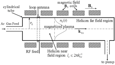
Figure 1: Schematic diagram of the helicon plasma source

In this paper, we consider the far-field region of the helicon wave, where the helicon wave is the travelling wave along the magnetic field direction. The electric, $\mathbf{E}_{1}\left(r,z,t\right)$, and magnetic, $\mathbf{B}_{1}\left(r,z,t\right)$, fields of the helicon wave are given in this region by the relations

$$\displaystyle E_{1r}\left(r,z,t\right)=E_{1r}\left(r\right)\sin\left(k_{0z}z-\omega_{0}t\right),$$

$$\displaystyle E_{1\varphi}\left(r,z,t\right)=E_{1\varphi}\left(r\right)\cos\left(k_{0z}z-\omega_{0}t\right),$$

$$\displaystyle E_{1z}\left(r,z,t\right)=0,$$ (4)

where $E_{1r}$ is the radial, $E_{1\varphi}$ is the azimuthal components of the electric field $\mathbf{E}_{1}\left(r,\varphi,z,t\right)$ of the helicon wave, $\omega_{0}$ is the frequency and $k_{0z}$ is the wavenumber component of the helicon wave directed along magnetic field $\mathbf{B}_{0}=B_{0}\mathbf{e}_{z}$ ;

$$\displaystyle B_{1r}\left(r,z,t\right)=B_{1r}\left(r\right)\cos\left(k_{0z}z-\omega_{0}t\right),$$

$$\displaystyle B_{1\varphi}\left(r,z,t\right)=B_{1\varphi}\left(r\right)\sin\left(k_{0z}z-\omega_{0}t\right),$$

$$\displaystyle B_{1z}\left(r,z,t\right)=B_{1z}\left(r\right)\sin\left(k_{0z}z-\omega_{0}t\right),$$ (5)

are the components of the magnetic field of the helicon wave. Note, that because magnetic field $\mathbf{B}_{1}$ satisfies the Gauss law $\nabla\cdot\mathbf{B}_{1}=0$, the relation

$$\displaystyle\frac{1}{r}\frac{\partial}{\partial r}\left(rB_{1r}\left(r\right)\right)+k_{0z}B_{1z}\left(r\right)=0$$ (6)

for ${B}_{1r}\left(r\right)$ and ${B}_{1z}\left(r\right)$ functions in Eq. (5) occurs.

The helicon wave field under the loop antenna and in its near-field, which is limited by the small distance $|l_{z}|\sim k^{-1}_{0z}$, has much more complicate spatial distribution along magnetic field and contains the propagating and the exponentially decaying modesGushchin . In this narrow near-field zone, where the helicon wave electric field has the maximum values of the magnitude and has maximum gradient along the magnetic field, the strong ponderomotive force along the magnetic fieldKarpman develops. This ponderomotive force determines the specific nonlinear processes of the helicon wave-plasma interactions, which are not investigated yet, that are different from the processes in the far-field region considered in this paper.

In the helicon wave field (4), (5), a plasma in equilibrium has an azimuthally symmetric radially inhomogeneous density profile. The radial profiles of the electric and magnetic fields depends on the plasma density profiles and differ from the profiles

$$\displaystyle E_{1r}\left(r\right)=E_{1r}J_{1}\left(k_{0\perp}r\right),$$

$$\displaystyle E_{1\varphi}\left(r\right)=E_{1\varphi}J_{1}\left(k_{0\perp}r\right),$$

$$\displaystyle B_{1r}\left(r\right)=B_{1r}J_{1}\left(k_{0\perp}r\right),$$

$$\displaystyle B_{1\varphi}\left(r\right)=B_{1\varphi}J_{1}\left(k_{0\perp}r\right),$$

$$\displaystyle B_{1z}\left(r\right)=B_{1z}J_{0}\left(k_{0\perp}r\right),$$ (7)

where $k_{0\perp}=\omega_{0}\omega_{pe}^{2}/\left(\omega_{ce}k_{0z}c^{2}\right)$, and $J_{0,1}\left(k_{0\perp}r\right)$ are the Bessel functions, known for the helicon plasmas with a uniform densityChen2 . The simple relations

$$\displaystyle B_{1\varphi}=\frac{ck_{0z}}{\omega_{0}}E_{1r},\quad B_{1r}=-\frac{ck_{0z}}{\omega_{0}}E_{1\varphi},$$ (8)

which stem from the Faradey’s law, reveal that the $B_{1r}$ and $B_{1\varphi}$ contained terms of the Lorentz force in Eq. (1),

$$\displaystyle\left|-\frac{v_{z}}{c}B_{1\varphi}\right|=\left|-\frac{v_{z}k_{0z}}{\omega_{0}}E_{1r}\right|\ll\left|E_{1r}\right|$$ (9)

and

$$\displaystyle\left|-\frac{v_{z}}{c}B_{1r}\right|=\left|-\frac{v_{z}k_{0z}}{\omega_{0}}E_{1\varphi}\right|\ll\left|E_{1\varphi}\right|$$ (10)

are much less than the helicon electric field force because $|\omega_{0}|\gg|k_{0z}v_{Te}|$ for the helicon wave, and may be neglected in the Vlasov equation (1). Without these terms, the simplified Vlasov equation with electron velocity $\mathbf{v}=\left(v_{\bot},\phi,v_{z}\right)$, determined in the polar coordinates by the relations (see Fig. 1)

$$\displaystyle v_{r}=v_{\bot}\cos\phi,\qquad v_{\varphi}=v_{\bot}\sin\phi,$$ (11)

where $v_{\bot}=\left(v_{r}^{2}+v_{\varphi}^{2}\right)^{1/2}$, and $\phi=\tan^{-1}\left(v_{\varphi}/v_{r}\right)$ is the gyroangle, has a form

$$\displaystyle\frac{\partial F_{e}}{\partial t}+v_{\perp}\cos\phi\frac{\partial F_{e}}{\partial r}+\frac{v_{\perp}}{r}\sin\phi\frac{\partial F_{e}}{\partial\varphi}+v_{z}\frac{\partial F_{e}}{\partial z}$$

$$\displaystyle+\frac{e}{m_{e}}\left(\sin\phi E_{\varphi}+\cos\phi E_{r}\right)\frac{\partial F_{e}}{\partial v_{\bot}}$$

$$\displaystyle-\left[\omega_{ce}+\frac{v_{\perp}}{r}\sin\phi+\frac{e}{m_{e}v_{\bot}}\left(\sin\phi E_{r}-\cos\phi E_{\varphi}\right)\right.$$

$$\displaystyle\left.+\frac{eB_{1z}\left(r,z,t\right)}{m_{e}c}\right]\frac{\partial F_{e}}{\partial\phi}+\frac{e}{m_{e}}E_{z}\frac{\partial F_{e}}{\partial v_{z}}=0.$$ (12)

The solution of the Vlasov equation (12) is presented in the next section.

III The theory of the micro-instabilities of the inhomogeneous cylindrical plasma in the field of the azimuthally symmetric radially inhomogeneous helicon wave

Helicon discharges contain two disparate spatial scales: the macroscale of the radial inhomogeneity of the helicon wave, which is commensurable with radial scale of the plasma density inhomogeneity, and the microscale, which is commensurable with the thermal Larmor radius of electrons, but is much less than the macroscale of the plasma and of the helicon wave inhomogeneities. In this section, we develop the two-scale approach to the analytical solution of the Vlasov equation (12), in which the respond on both spatial scales of the cylindrical radially inhomogeneous plasma on the azimuthally symmetric radially inhomogeneous helicon wave is accounted for. This two-scale approach is based on the employing of the cylindrical guiding center variables $R_{e},\psi$, and of the electron Larmor orbit variables $\rho_{e},\delta$, which are related to the original electron variables $r,\varphi,v_{\bot},\phi$ via Chibisov

$$\displaystyle R_{e}^{2}=\frac{1}{\omega_{ce}^{2}}\left(v^{2}_{\perp}+2v_{\perp}r\omega_{ce}\sin\phi+r^{2}\omega_{ce}^{2}\right),$$ (13)

$$\displaystyle\psi=\varphi-\alpha,$$ (14)

$$\displaystyle\rho^{2}_{e}=\frac{v_{\perp}^{2}}{\omega_{ce}^{2}},$$ (15)

$$\displaystyle\delta=\phi+\alpha,$$ (16)

$$\displaystyle\alpha=\arcsin\left[\frac{\cos\phi}{\left(1+v^{-2}_{\perp}\left(r^{2}\omega_{ce}^{2}+2v_{\perp}r\omega_{ce}\sin\phi\right)\right)^{1/2}}\right].$$

The geometric interpretation of the cylindrical guiding center coordinates for an electron is presented in Fig. 1. In coordinates $R_{e}$, $\psi$, $\rho_{e}$, $\delta$, $z$, $t$, Eq. (12) transforms to the following equation for $F_{e}\left(R_{e},\psi,\rho_{e},\delta,z,t\right)$:

$$\displaystyle\frac{\partial F_{e}}{\partial t}+v_{z}\frac{\partial F_{e}}{\partial z}-\omega_{ce}\frac{\partial F_{e}}{\partial\delta}$$

$$\displaystyle+\frac{c}{B_{0}}\frac{1}{\left(R^{2}_{e}-2\rho_{e}R_{e}\sin\delta+\rho^{2}_{e}\right)^{1/2}}$$

$$\displaystyle\times\left[\left(E_{1r}\rho_{e}\cos\delta+E_{1\varphi}\left(R_{e}-\rho_{e}\sin\delta\right)\right)\frac{\partial F_{e}}{\partial R_{e}}\right.$$

$$\displaystyle-\left.\left(\left(1-\frac{\rho_{e}}{R_{e}}\sin\delta\right)E_{1r}+\frac{\rho_{e}}{R_{e}}\cos\delta E_{1\varphi}\right)\frac{\partial F_{e}}{\partial\psi}\right.$$

$$\displaystyle\left.+\left(E_{1r}R_{e}\cos\delta+E_{1\varphi}\left(R_{e}\sin\delta-\rho_{e}\right)\right)\frac{\partial F_{e}}{\partial\rho_{e}}\right.$$

$$\displaystyle+\left(E_{1r}\left(2-\sin\delta\frac{\left(R^{2}_{e}+\rho^{2}_{e}\right)}{R_{e}\rho_{e}}\right)\left.+E_{1\varphi}\cos\delta\frac{\left(R^{2}_{e}+\rho^{2}_{e}\right)}{R_{e}\rho_{e}}\right)\frac{\partial F_{e}}{\partial\delta}\right]$$

$$\displaystyle-\frac{e}{m_{e}c}B_{1z}\left[\rho_{e}\cos\delta\frac{\partial F_{e}}{\partial R_{e}}+\frac{\partial F_{e}}{\partial\delta}-\sin\delta\frac{\rho_{e}}{R_{e}}\left(\frac{\partial F_{e}}{\partial\delta}-\frac{\partial F_{e}}{\partial\psi}\right)\right]$$

$$\displaystyle-\frac{c}{B_{0}R_{e}}\left(\frac{\partial\Phi}{\partial\psi}-\frac{\partial\Phi}{\partial\delta}\right)\frac{\partial F_{e}}{\partial R_{e}}+\frac{c}{B_{0}\rho_{e}}\frac{\partial\Phi}{\partial\delta}\frac{\partial F_{e}}{\partial\rho_{e}}-\frac{e}{m_{e}}\frac{\partial\Phi}{\partial z}\frac{\partial F_{e}}{\partial v_{ez}}=0.$$ (17)

In the helicon discharge, $\rho_{e}\ll R_{e}$, excluding small region $R_{e}\sim\rho_{e}$ of the discharge center. For example, for the magnetic field $B_{0}=50$ mT and electron temperature $T_{e}=4$ eV the thermal electron Larmor radius $\rho_{e}=10^{-1}$ cm, whereas the radial scales of the helicon wave and of a plasma inhomogeneities are typically a few centimetres. Equation (17), in which the terms on the order of $\rho_{e}/R_{e}\ll 1$ are omitted, becomes

$$\displaystyle\frac{\partial F_{e}}{\partial t}+v_{z}\frac{\partial F_{e}}{\partial z}+\frac{c}{B_{0}}E_{1\varphi}\frac{\partial F_{e}}{\partial R_{e}}-\frac{c}{B_{0}}E_{1r}\frac{\partial F_{e}}{R_{e}\partial\psi}$$

$$\displaystyle+\frac{c}{B_{0}}\left(E_{1r}\cos\delta+E_{1\varphi}\sin\delta\right)\frac{\partial F_{e}}{\partial\rho_{e}}$$

$$\displaystyle+\left(2\frac{c}{B_{0}R_{e}}E_{1r}-\omega_{ce}-\frac{c}{B_{0}\rho_{e}}\frac{1}{\rho_{e}}\left(E_{1r}\sin\delta-E_{1\varphi}\cos\delta\right)\right)\frac{\partial F_{e}}{\partial\delta}$$

$$\displaystyle-\frac{e}{m_{e}c}B_{1z}\frac{\partial F_{e}}{\rho_{e}\partial\delta}=\frac{c}{B_{0}R_{e}}\left(\frac{\partial\Phi}{\partial\psi}-\frac{\partial\Phi}{\partial\delta}\right)\frac{\partial F_{e}}{\partial R_{e}}$$

$$\displaystyle-\frac{c}{B_{0}\rho_{e}}\frac{\partial\Phi}{\partial\delta}\frac{\partial F_{e}}{\partial\rho_{e}}+\frac{e}{m_{e}}\frac{\partial\Phi}{\partial z}\frac{\partial F_{e}}{\partial v_{ez}}.$$ (18)

The Vlasov equation (18) with $\Phi=0$ is the equation for the equilibrium electron distribution function $F_{e0}$. Consider now the system of equations for the characteristics of equation for $F_{e0}$,

$$\displaystyle dt=\frac{dR_{e}}{\frac{c}{B_{0}}E_{1\varphi}}=\frac{d\psi}{-\frac{c}{B_{0}R_{e}}E_{1r}}=\frac{d\rho_{e}}{\frac{c}{B_{0}}\left(E_{1r}\cos\delta+E_{1\varphi}\sin\delta\right)}$$

$$\displaystyle=d\delta\left[-\omega_{ce}+2\frac{c}{B_{0}R_{e}}E_{1r}-\frac{eB_{1z}}{cm_{e}}\right.$$

$$\displaystyle\left.-\frac{c}{B_{0}\rho_{e}}\left(E_{1r}\sin\delta-E_{1\varphi}\cos\delta\right)\right]^{-1}=\frac{dz}{v_{z}}.$$ (19)

With approximations $E_{1r}\left(r\right)\approx E_{1r}\left(R_{e}\right)$ and $E_{1\varphi}\left(r\right)\approx E_{1\varphi}\left(R_{e}\right)$, which follows from the relation

$$\displaystyle r=\left(R^{2}_{e}-2\rho_{e}R_{e}\sin\delta+\rho^{2}_{e}\right)^{1/2}\approx R_{e}$$ (20)

in the limit $\rho_{e}\ll R_{e}$, the system of equations for the macroscale guiding center coordinates $R_{e}$, $\psi$

$$\displaystyle dt=\frac{dR_{e}}{\frac{c}{B_{0}}E_{1\varphi}\left(R_{e}\right)\cos\left(\omega_{0}t-k_{0z}\left(z_{1}+v_{z}t\right)\right)}$$

$$\displaystyle=\frac{d\psi}{-\frac{c}{B_{0}R_{e}}E_{1r}\left(R_{e}\right)\sin\left(\omega_{0}t-k_{0z}\left(z_{1}+v_{z}t\right)\right)},$$ (21)

where $z_{1}=z-v_{z}t$ is the integral of system (19), becomes separate from the system of equation for the microscale coordinates $\rho_{e}$ and $\delta$ of the Larmor motion. By direct integration of Eq. (21) for $R_{e}\left(t\right)$ and for $\psi\left(t\right)$ we derive the equations

$$\displaystyle R_{e1}=R_{e}\left(t\right)-\frac{c}{B_{0}}\int dt_{1}E_{1\varphi}\left(R_{e}\left(t_{1}\right)\right)\cos\left(\omega_{0}t_{1}-k_{0z}\left(z_{1}+v_{z}t_{1}\right)\right)$$ (22)

and

$$\displaystyle\psi_{1}=\psi\left(t\right)+\frac{c}{B_{0}}\int dt_{1}\frac{1}{R_{e}\left(t_{1}\right)}E_{1r}\left(R_{e}\left(t_{1}\right)\right)\sin\left(\omega_{0}t_{1}-k_{0z}\left(z_{1}+v_{z}t_{1}\right)\right),$$ (23)

where $R_{e1}$ and $\psi_{1}$ are the integrals of system (21). By employing the method of successive approximation we derive the approximate solution of Eq. (22) for $R_{e}\left(t\right)$ in the form

$$\displaystyle R_{e}\left(t\right)\approx R_{e1}+\frac{c}{B_{0}\omega_{0}}E_{1\varphi}\left(R_{e1}\right)\sin\left(\omega_{0}t-k_{0z}z_{1}\right)$$

$$\displaystyle-\frac{c^{2}}{B_{0}^{2}\omega_{0}^{2}}\frac{1}{4}\sin^{2}\left(\omega_{0}t-k_{0z}z_{1}\right)\frac{d}{dR_{e1}}E_{1\varphi}^{2}\left(R_{e1}\right),$$ (24)

which is the power series expansion in $\left|\xi/R_{e1}\right|\ll 1$, where $\xi=\frac{c}{B_{0}\omega_{0}}E_{1\varphi}\left(R_{e1}\right)$ is the amplitude of the displacement of an electron along the coordinate $R_{e}$ at $R_{e}=R_{e1}$. In this solution, the term $k_{0z}v_{z}t$ is omitted, because for the helicon wave $\omega_{0}\gg k_{0z}v_{Te}$, where $v_{Te}$ is the electron thermal velocity.

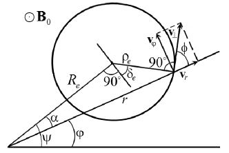
Figure 2: The geometric interpretation of the cylindrical guiding center coordinates for an electron.

The approximate solution to Eq. (23) for the angle $\psi$ in the form of the power series expansion in $\left|\xi/R_{e1}\right|\ll 1$ with accounting for the terms on the first and the second order of $\left|\xi/R_{e1}\right|^{2}$ has a form

$$\displaystyle\psi\approx\psi_{1}-\frac{c}{B_{0}R_{e1}\omega_{0}}E_{1r}\left(R_{e1}\right)\cos\left(\omega_{0}t-k_{z0}z_{1}\right)$$

$$\displaystyle-\frac{c^{2}E_{1\varphi}\left(R_{e1}\right)}{2B_{0}^{2}R_{e1}^{2}\omega_{0}}\left(E_{1r}\left(R_{e1}\right)-R_{e1}\frac{\partial E_{1r}\left(R_{e1}\right)}{\partial R_{e1}}\right)$$

$$\displaystyle\times\left[t-\frac{1}{2\omega_{0}}\sin 2\left(\omega_{0}t-k_{z0}z_{1}\right)\right].$$ (25)

It contains the terms oscillating on frequencies $\omega_{0}$ and $2\omega_{0}$, and the term corresponding to the rotation of the guiding center coordinate with stationary radially inhomogeneous angular velocity $\Omega_{e}\left(R_{e1}\right)$,

$$\displaystyle\Omega_{e}\left(R_{e1}\right)=\frac{c^{2}E_{1\varphi}\left(R_{e1}\right)}{2B_{0}^{2}R_{e1}^{2}\omega_{0}}\left[E_{1r}\left(R_{e1}\right)-R_{e1}\frac{\partial E_{1r}\left(R_{e1}\right)}{\partial R_{e1}}\right].$$ (26)

The discovered effect of the electron component rotation with angular velocity $\Omega_{e}\left(R_{e1}\right)$ in the cylindrical azimuthally symmetric $\left(m_{0}=0\right)$ helicon wave is the first result of our two-scales analysis of the Vlasov equation solution.This effect is missed in the slab model of plasma in the spatially uniform helicon wave field. The order on value estimate for $B_{0}=50$ mT, $\omega_{0}=10^{7}$ s^-1, $E_{1r}=E_{1\varphi}=5$ V/cm, and $R_{e1}=2.5$ cm gives $\Omega_{e}=8\cdot 10^{5}$ s^-1. In what follows, we use the approximation

$$\displaystyle\psi=\psi_{1}-a_{e}\left(R_{e1}\right)\cos\left(\omega_{0}t-k_{0z}z_{1}\right)-\Omega_{e}\left(R_{e1}\right)t,$$ (27)

where

$$\displaystyle a_{e}\left(R_{e1}\right)=\frac{cE_{1r}\left(R_{e1}\right)}{B_{0}R_{e1}\omega_{0}},$$ (28)

which is valid for a time $t\sim\Omega_{0}^{-1}\gg\omega_{0}^{-1}$.

Because $\omega_{ce}$ is much larger than any other term in the equation for $d\delta/dt$ of system (19), the solution for $\delta_{1}$ is determined with a great accuracy as

$$\displaystyle\delta=\delta_{1}-\omega_{ce}t.$$ (29)

The solution of the equation for the radius $\rho_{e}$ of the electron Larmor orbit,

$$\displaystyle\frac{d\rho_{e}}{dt}=\frac{c}{B_{0}}\Big{[}E_{1r}\left(R_{e}\right)\sin\left(k_{z0}z_{1}-\omega_{0}t\right)\cos\left(\delta_{1}-\omega_{ce}t\right)$$

$$\displaystyle+E_{1\varphi}\left(R_{e}\right)\cos\left(\omega_{0}t-k_{z0}z_{1}\right)\sin\left(\delta_{1}-\omega_{ce}t\right)\Big{]},$$ (30)

where $\delta_{1}$ is given by Eq. (29), is

$$\displaystyle\rho_{e}=\rho_{e1}-\frac{c}{B_{0}\omega_{ce}}\Big{[}E_{1r}\left(R_{e1}\right)\sin\left(\omega_{0}t-k_{z0}z_{1}\right)\sin\left(\omega_{ce}t-\delta_{1}\right)$$

$$\displaystyle-E_{1\varphi}\left(R_{e1}\right)\cos\left(\omega_{0}t-k_{z0}z_{1}\right)\cos\left(\omega_{ce}t-\delta_{1}\right)\Big{]}$$ (31)

with accuracy to terms of the order of $O\left(\frac{\omega_{0}}{\omega_{ce}}\ll 1\right)$.

It is easy to check that the Vlasov equation for the equilibrium electron distribution function $F_{e0}$ in variables $R_{e1},\psi_{1},\rho_{e1},\delta_{1},v_{z},z_{1}$ determined by the solutions (24), (25), (31) and (29), respectively, reduces to the equation

$$\displaystyle\frac{\partial F_{e0}}{\partial t}=0,$$

and, therefore, $F_{e0}=F_{e0}\left(R_{e1},\psi_{1},\rho_{e1},\delta_{1},v_{z},z_{1}\right)$, and does not depend on time variable. The equation for the perturbation $f_{e}\left(R_{e1},\psi_{1},\rho_{e1},\delta_{1},v_{z},z_{1},t\right)$ of the equilibrium distribution function $F_{e0}\left(R_{e1},\rho_{e1},v_{z}\right)$ of the azimuthally symmetric radially inhomogeneous plasma,

$$\displaystyle\frac{d}{dt}f_{e}\left(R_{e1},\psi_{1},\rho_{e1},\delta_{1},v_{z},z_{1},t\right)=\left(\frac{c}{B_{0}R_{e1}}\left(\frac{\partial\Phi}{\partial\psi_{1}}-\frac{\partial\Phi}{\partial\delta_{1}}\right)\frac{\partial}{\partial R_{e1}}\right.$$

$$\displaystyle\left.-\frac{c}{B_{0}}\frac{1}{\rho_{e1}}\frac{\partial\Phi}{\partial\delta_{1}}\frac{\partial}{\partial\rho_{e1}}+\frac{e}{m_{e}}\frac{\partial\Phi}{\partial z_{1}}\frac{\partial}{\partial v_{ez}}\right)F_{e0}\left(R_{e1},\rho_{e1},v_{z}\right).$$ (32)

follows from Eq. (18) in which variables $R_{e},\psi,\rho_{e},\delta,v_{z},z,t$ are transformed on
$R_{e1},\psi_{1},\rho_{e1},\delta_{1},v_{z},z_{1},t$, by employing the relations (24), (25), (27), (29), (31). In this equation, potential $\Phi\left(R_{e1},\psi_{1},\rho_{e1},\delta_{1},v_{z},z_{1},t\right)$ is presented in the form of the Fourier-Bessel transformation,

$$\displaystyle\Phi\left(R_{e1},\psi_{1},\rho_{e1},\delta_{1},v_{z},z_{1},t\right)=\frac{1}{\left(2\pi\right)^{4}}\sum\limits^{\infty}_{m=-\infty}\sum\limits^{\infty}_{n=-\infty}$$

$$\displaystyle\times\int dk_{\perp}k_{\perp}dk_{z}d\theta d\omega\Phi\left(k_{\perp},\theta,k_{z},\omega\right)J_{n}\left(k_{\perp}\rho_{e1}\right)J_{n+m}\left(k_{\perp}R_{e1}\right)$$

$$\displaystyle\times\exp\left[-in\left(\delta_{1}-\omega_{ce}t\right)-im\left(\theta-\psi_{1}+a_{e}\left(R_{e1}\right)\cos\left(\omega_{0}t-k_{0z}z_{1}\right)+\Omega_{e}\left(R_{e1}\right)t\right)\right.$$

$$\displaystyle\left.+i\left(m+n\right)\frac{\pi}{2}-i\left(\omega-k_{z}v_{z}\right)t+ik_{z}z_{1}\right].$$ (33)

It was derived from the Fourier-Bessel transform

$$\displaystyle\Phi\left(r,\varphi,z,t\right)=\frac{1}{\left(2\pi\right)^{4}}\int\Phi\left(\mathbf{k},\omega\right)e^{-i\omega t+ik_{\perp}r\cos\left(\theta-\varphi\right)+ik_{z}z}k_{\perp}dk_{\perp}d\theta dk_{z}d\omega,$$ (34)

in which the identity

$$\displaystyle k_{\perp}r\cos\left(\theta-\varphi\right)=k_{\perp}R_{e}\cos\left(\theta-\psi\right)+k_{\perp}\rho_{e}\sin\left(\theta-\psi-\delta\right)$$ (35)

and Eqs. (27) and (29) were employed. The solution for $f_{e}\left(R_{e1},\psi_{1},\rho_{e1},\delta_{1},v_{z},z_{1},t\right)$ of Eq. (32) with potential (33) is

$$\displaystyle f_{e}\left(R_{e1},\psi_{1},\rho_{e1},\delta_{1},v_{z},z_{1},t\right)=-\frac{1}{\left(2\pi\right)^{4}}\sum\limits_{m=-\infty}^{\infty}\sum\limits_{n=-\infty}^{\infty}\sum\limits_{p=-\infty}^{\infty}\int dk_{\bot}k_{\bot}d\theta dk_{z}d\omega\Phi\left(\mathbf{k},\omega\right)$$

$$\displaystyle\times\frac{J_{n}\left(k_{\bot}\rho_{e1}\right)J_{m+n}\left(k_{\bot}R_{e1}\right)J_{p}\left(ma_{e}\left(R_{e1}\right)\right)}{\omega-k_{z}v_{z}-n\omega_{ce}-p\omega_{0}+m\Omega_{e}\left(R_{e1}\right)}$$

$$\displaystyle\times\left[\frac{c}{B_{0}}\left(\left(m+n\right)\frac{1}{R_{e1}}\frac{\partial F_{e0}}{\partial R_{e1}}+n\frac{1}{\rho_{e1}}\frac{\partial F_{e0}}{\partial\rho_{e1}}\right)+\frac{e}{m_{e}}k_{z}\frac{\partial F_{e0}}{\partial v_{ez}}\right]$$

$$\displaystyle\times\exp\left(-i\left(\omega-k_{z}v_{z}-n\omega_{ce}-p\omega_{0}+m\Omega_{e}\left(R_{e1}\right)\right)t-in\delta_{1}-im\left(\theta-\psi_{1}\right)\right.$$

$$\displaystyle\left.+i\left(k_{z}-pk_{0z}\right)z_{1}+i\left(m+n-p\right)\frac{\pi}{2}\right).$$ (36)

The dynamics of ions in the helicon wave is different from the electron dynamics. The ion cyclotron frequency, $\omega_{ci}$, is much less than the frequency of the helicon wave $\omega_{0}$. (For the magnetic field $B_{0}=50$ mT and argon gas $\omega_{ci}=1.25\cdot 10^{4}$s^-1 $\ll\omega_{0}=10^{7}$s^-1 ). Therefore, the ions displacement in the helicon wave is as of the unmagnetized particle, and is estimated by $\delta r_{i}\sim e_{i}E_{1}/m_{i}\omega^{2}_{0}\sim 10^{-3}$cm for $E_{1}=5$ V/cm. This displacement is much less than the thermal argon ion Larmor radius $\rho_{i}$, which for $T_{i}=2.6\cdot 10$ ^-2 eV and $B_{0}=50$ mT is on the order of 2 cm. Therefore, the thermal motion of ions is practically unaffected by the helicon wave.

By using the solution (36) for $f_{e}$ in the Poisson equation (3), we derive the integral equation for the $m$-th harmonic $\Phi_{m}\left(k_{\bot},k_{z},\omega\right)$ of the Fourier-Bessel transformed potential determined by the relation

$$\displaystyle\Phi_{m}\left(k_{\bot},k_{z},\omega\right)=\frac{1}{2\pi}\int d\theta_{1}\Phi\left(k_{\bot},\theta_{1},k_{z},\omega\right)e^{-im\theta_{1}}.$$ (37)

This equation has a form

$$\displaystyle\Phi_{m}\left(k_{\bot},k_{z},\omega\right)\left(1-\frac{\omega^{2}_{pi}}{\omega^{2}}\right)$$

$$\displaystyle+8\pi^{2}\frac{e^{2}}{k^{2}m_{e}}\omega^{2}_{ce}\sum^{\infty}_{n=-\infty}\sum^{\infty}_{p=-\infty}\sum^{\infty}_{p_{1}=-\infty}\int\limits^{\infty}_{0}dR_{e1}R_{e1}\int\limits^{\infty}_{0}d\rho_{e1}\rho_{e1}\int\limits^{\infty}_{-\infty}dv_{z}$$

$$\displaystyle\times\int\limits_{0}^{\infty}dk_{1\bot}k_{1\bot}\Phi_{m}\left(k_{1\bot},k_{z}-\left(p-p_{1}\right)k_{0z},\omega-\left(p-p_{1}\right)\omega_{0}\right)e^{i\left(p-p_{1}\right)\frac{\pi}{2}}$$

$$\displaystyle\times\frac{J_{n}\left(k_{\bot}\rho_{e1}\right)J_{n}\left(k_{1\bot}\rho_{e1}\right)J_{n+m}\left(k_{\bot}R_{e1}\right)J_{n+m}\left(k_{1\bot}R_{e1}\right)J_{p}\left(ma_{e}\left(R_{e1}\right)\right)J_{p_{1}}\left(ma_{e}\left(R_{e1}\right)\right)}{\omega-n\omega_{ce}-p\omega_{0}-k_{z}v_{z}+m\Omega_{e}\left(R_{e1}\right)}$$

$$\displaystyle\times\left[\frac{\left(m+n\right)}{\omega_{ce}R_{e1}}\frac{\partial F_{e0}}{\partial R_{e1}}+\frac{n}{\omega_{ce}\rho_{e1}}\frac{\partial F_{e0}}{\partial\rho_{e1}}+k_{z}\frac{\partial F_{e0}}{\partial v_{z}}\right]=0.$$ (38)

In Eq. (38), the approximation of the unmagnetized ions was used, which is applicable for the treating of the instabilities with the growth rate $\gamma\left(\mathbf{k}\right)\gg\omega_{ci}/2\pi$ and $k_{\bot}\rho_{i}\gg 1$. The solution to Eq. (38) for $\Phi_{m}\left(k_{\bot},k_{z},\omega\right)$ is the cylindrical wave with a continuous spectrum characterized by the wave number $k_{\bot}$ and azimuthal number $m$. Here, we derive the solution to Eq. (38) in the short wavelength limit

$$\displaystyle k_{\bot}R_{e1}\sim m\gg 1,$$ (39)

employing the approach developed in Ref. Mikhailenko2 in the studies of the drift turbulence of the azimuthally symmetric radially nonuniform plasma and applied in Ref.Mikhailenko3 in the studies of the shear flow driven ion cyclotron and ion acoustic instabilities of the cylindrical inhomogeneous plasma. The integration over macroscale $R_{e1}$ and over microscale wave number $k_{1\bot}$, performed in Ref.Mikhailenko2 , reveal that the vicinity of the $R_{e1}=\frac{m}{k_{1\bot}}=R_{e0}$ values and the vicinity of the $k_{1\bot}=k_{\bot}$ values give the dominant input to the integrals over $R_{e1}$ and $k_{1\bot}$ in Eq. (38). It is important to note, that the region of $R_{e1}\approx R_{e0}$ corresponds approximately to the region of the first maximum of the $J_{m}\left(k_{\bot}R_{e1}\right)$ Bessel function, where the known cosine asymptotic, which is valid for $k_{\bot}R_{e1}\gg m$, is not applicable, and Eq. (38) can not be approximated by the plane geometry model. After the integration over $R_{e1}$ and $k_{1\bot}$, Eq. (38) becomes

$$\displaystyle\Phi_{m}\left(k_{\bot},k_{z},\omega\right)\left(1-\frac{\omega^{2}_{pi}}{\omega^{2}}\right)$$

$$\displaystyle+8\pi^{2}\frac{e^{2}}{k^{2}m_{e}}\omega^{2}_{ce}\sum^{\infty}_{n=-\infty}\sum^{\infty}_{p=-\infty}\sum^{\infty}_{p_{1}=-\infty}\int\limits^{\infty}_{0}d\rho_{e1}\rho_{e1}\int\limits^{\infty}_{-\infty}dv_{z}$$

$$\displaystyle\times\Phi_{m}\left(k_{\bot},k_{z}-\left(p-p_{1}\right)k_{0z},\omega-\left(p-p_{1}\right)\omega_{0}\right)e^{i\left(p-p_{1}\right)\frac{\pi}{2}}$$

$$\displaystyle\times\frac{J^{2}_{n}\left(k_{\bot}\rho_{e1}\right)J_{p}\left(ma_{e}\left(R_{e0}\right)\right)J_{p_{1}}\left(ma_{e}\left(R_{e0}\right)\right)}{\omega-n\omega_{ce}-p\omega_{0}-k_{z}v_{z}+m\Omega_{e}\left(R_{e0}\right)}$$

$$\displaystyle\times\left[\frac{\left(m+n\right)}{\omega_{ce}R_{e0}}\frac{\partial F_{e0}}{\partial R_{e0}}+\frac{n}{\omega_{ce}\rho_{e1}}\frac{\partial F_{e0}}{\partial\rho_{e1}}+k_{z}\frac{\partial F_{e0}}{\partial v_{z}}\right]=0.$$ (40)

The cylindrical plasma excited by the cylindrical azimuthally symmetric $\left(m_{0}=0\right)$ helicon wave has an azimuthally symmetric radially inhomogeneous density and temperature profiles. We will consider in what follows the equilibrium distribution function $F_{e0}\left(\rho_{e1},v_{z},R_{e0}\right)$ for Eq. (40) as a Maxwellian

$$\displaystyle F_{e0}\left(\rho_{e1},v_{z},R_{e0}\right)=\frac{n_{e0}\left(R_{e0}\right)}{\left(2\pi\right)^{3/2}v^{3}_{Te}}\exp\left[-\frac{\rho^{2}_{e1}}{2\rho^{2}_{Te}}-\frac{v^{2}_{z}}{v^{2}_{Te}}\right],$$ (41)

where $\rho_{Te}=v_{Te}\left(R_{e0}\right)/\omega_{ce}$, and $v^{2}_{Te}\left(R_{e0}\right)=T_{e}\left(R_{e0}\right)/m_{e}$. After integration of Eq. (40) over $\rho_{e1}$ and $v_{z}$ with Maxwellian distribution (41), we derive the basic equation for $\Phi_{m}\left(k_{\bot},k_{z},\omega\right)$,

$$\displaystyle\Phi_{m}\left(k_{\bot},k_{z},\omega\right)\left(1-\frac{\omega^{2}_{pi}}{\omega^{2}}\right)$$

$$\displaystyle+\sum^{\infty}_{p=-\infty}\sum^{\infty}_{p_{1}=-\infty}J_{p}\left(ma_{e}\left(R_{e0}\right)\right)J_{p_{1}}\left(ma_{e}\left(R_{e0}\right)\right)$$

$$\displaystyle\times\Phi_{m}\left(k_{\bot},k_{z}-\left(p-p_{1}\right)k_{0z},\omega-\left(p-p_{1}\right)\omega_{0}\right)e^{i\left(p-p_{1}\right)\frac{\pi}{2}}$$

$$\displaystyle\times\varepsilon_{m(e)}\left(k_{\bot},k_{z},\omega-p\omega_{0}\right)=0,$$ (42)

where

$$\displaystyle\varepsilon_{m(e)}\left(k_{\bot},k_{z},\omega-p\omega_{0}\right)$$

$$\displaystyle=\frac{1}{k^{2}\lambda^{2}_{De}}\left\{1+i\sqrt{\pi}\sum^{\infty}_{n=-\infty}\left(\omega+m\Omega_{e}\left(R_{e0}\right)-p\omega_{0}-\left(m+n\right)\omega_{de}\left(R_{e0}\right)\left(1-\frac{1}{2}\eta_{e}\right)\right)\right.$$

$$\displaystyle\left.\times\frac{1}{\sqrt{2}k_{z}v_{Te}}W\left(z_{en,p}\right)I_{n}\left(k_{\bot}^{2}\rho^{2}_{e}\right)e^{-k_{\bot}^{2}\rho^{2}_{e}}\right.$$

$$\displaystyle\left.-\eta_{e}\sum^{\infty}_{n=-\infty}\frac{\left(m+n\right)\omega_{de}\left(R_{e0}\right)}{\sqrt{2}k_{z}v_{Te}}e^{-k_{\bot}^{2}\rho^{2}_{e}}\left[z_{en,p}\left(1+i\sqrt{\pi}z_{en,p}W\left(z_{en,p}\right)\right)I_{n}\left(k_{\bot}^{2}\rho^{2}_{e}\right)\right.\right.$$

$$\displaystyle\left.\left.-i\sqrt{\pi}W\left(z_{en,p}\right)k_{\bot}^{2}\rho^{2}_{e}\left(I_{n}\left(k_{\bot}^{2}\rho^{2}_{e}\right)-I^{\prime}_{n}\left(k_{\bot}^{2}\rho^{2}_{e}\right)\right)\right]\right\}=0.$$ (43)

In Eq. (43), $\lambda_{De}$ is the electron Debye length, $W\left(z_{e}\right)=e^{-z_{e}^{2}}\left(1+\left(2i/\sqrt{\pi}\right)\int\limits_{0}^{z_{e}}e^{t^{2}}dt\right)$ is the Faddeeva functionFaddeyeva with argument $z_{e}$ equal to

$$\displaystyle z_{e}=\frac{\omega-p\omega_{0}+m\Omega_{e}\left(R_{e0}\right)-n\omega_{ce}}{\sqrt{2}k_{z}v_{Te}},$$ (44)

$I_{n}$ is the modified Bessel function of the first kind and order $n$, the prime in $I^{\prime}_{n}$ denotes the derivative with respect to the argument $k^{2}_{\bot}\rho^{2}_{Te}$ of the $I_{n}$ function, $\omega_{de}\left(R_{e0}\right)$ is the local electron diamagnetic drift frequency

$$\displaystyle\omega_{de}\left(R_{e0}\right)=\omega_{ce}\rho^{2}_{Te}\frac{\partial\ln n_{0e}\left(R_{e0}\right)}{R_{e0}\partial R_{e0}},$$ (45)

and $\eta_{e}=\partial\ln T_{e}/\partial\ln n_{e0}$.

Equation (42) is the basic equation, which determines in the short wavelength limit (39) the electrostatic respond of the cylindrical radially inhomogeneous plasma on the cylindrical helicon wave. Equation (42) is in fact the infinite system of equations for the potential $\Phi_{m}\left(k_{\bot},k_{z},\omega\right)$ and for the infinite number of satellites
$\Phi_{m}\left(k_{1\bot},k_{z}-\left(p-p_{1}\right)k_{0z},\omega-\left(p-p_{1}\right)\omega_{0}\right)$
of this potential, which are derived from Eq. (42) by changing in Eq. (42) $\omega$ on $\omega-\left(p-p_{1}\right)\omega_{0}$ and $k_{z}$ on $k_{z}-\left(p-p_{1}\right)k_{0z}$, where $p$ and $p_{1}$ are the integral numbers. The equality to zero of the determinant of this homogeneous system gives the general dispersion equation the solution of which determines the dispersive properties of the parametric instabilities.

It was found analytically for the slab plasma geometryAkhiezer ; Aliev , that the relative oscillating motion of electrons and ions under the action of the helicon wave with frequency $\omega_{0}$ is a source of the development of the instabilities of the parametric type. The motion of electrons in the field of the cylindrical radially inhomogeneous helicon wave is more complicate. It includes the oscillating of the electrons relative to ions and the rotating of the electron component relative to ions with radially inhomogeneous stationary angular velocity $\Omega\left(R_{e0}\right)$. Both these motions are included in Eq. (42), solution of which may be derived only numerically.

IV The ion acoustic instability of the cylindrical plasma in the field of the azimuthally symmetric helicon wave

For understanding the qualitative and the quantitative effect of the rotation of electrons with angular velocity $\Omega_{e}\left(R_{e0}\right)\ll\omega_{0}$ on the plasma stability we derive the simplest analytical solution to Eq. (42) in which terms with $p\neq p_{1}\neq 0$ are neglected. Equation (42) with $n=p=p_{1}=0$ in this case becomes

$$\displaystyle\Phi_{m}\left(k_{\bot},k_{z},\omega\right)\varepsilon_{m}\left(k_{\bot},k_{z},\omega\right)=0,$$ (46)

where

$$\displaystyle\varepsilon_{m}\left(k_{\bot},k_{z},\omega\right)=1-\frac{\omega^{2}_{pi}}{\omega^{2}}+J^{2}_{0}\left(ma_{e}\left(R_{e0}\right)\right)\frac{1}{k^{2}\lambda^{2}_{De}}\left\{1\right.$$

$$\displaystyle\left.+i\sqrt{\pi}\left(\omega+m\Omega_{e}\left(R_{e0}\right)-m\omega_{de}\left(1-\frac{1}{2}\eta_{e}\right)\right)\right.$$

$$\displaystyle\left.\times\frac{1}{\sqrt{2}k_{z}v_{Te}}W\left(z_{e0}\right)I_{0}\left(k_{\bot}^{2}\rho^{2}_{e}\right)e^{-k_{\bot}^{2}\rho^{2}_{e}}\right.$$

$$\displaystyle\left.-\eta_{e}\frac{m\omega_{de}}{\sqrt{2}k_{z}v_{Te}}e^{-k_{\bot}^{2}\rho^{2}_{e}}\left[z_{e0}\left(1+i\sqrt{\pi}z_{e0}W\left(z_{e0}\right)\right)I_{0}\left(k_{\bot}^{2}\rho^{2}_{e}\right)\right.\right.$$

$$\displaystyle\left.\left.-i\sqrt{\pi}W\left(z_{e0}\right)k_{\bot}^{2}\rho^{2}_{e}\left(I_{0}\left(k_{\bot}^{2}\rho^{2}_{e}\right)-I_{1}\left(k_{\bot}^{2}\rho^{2}_{e}\right)\right)\right]\right\},$$ (47)

in which

$$\displaystyle z_{e0}=\frac{\omega+m\Omega_{e}\left(R_{e0}\right)}{\sqrt{2}k_{z}v_{Te}}.$$ (48)

The solution to Eq. (46) is

$$\displaystyle\Phi_{m}\left(k_{\bot},k_{z},\omega\right)=\Phi_{m}\left(k_{\bot},k_{z},\omega_{m}\left(k_{\bot},k_{z}\right)\right)\delta\left(\omega-\omega_{m}\left(k_{\bot},k_{z}\right)\right)$$ (49)

for $\omega=\omega_{m}\left(k_{\bot},k_{z}\right)$ and $\Phi_{m}\left(k_{\bot},k_{z},\omega\right)=0$ for $\omega\neq\omega_{m}\left(k_{\bot},k_{z}\right)$, where $\omega_{m}\left(k_{\bot},k_{z}\right)$ is the solution to the equation

$$\displaystyle\varepsilon_{m}\left(k_{\bot},k_{z},\omega\right)=0.$$ (50)

The inverse Fourier-Bessel transform of solution (49)

$$\displaystyle\Phi_{m}\left(r,z,t\right)=\int dk_{z}dk_{\bot}\Phi_{m}\left(k_{\bot},k_{z},\omega\right)\delta\left(\omega-\omega_{m}\left(k_{\bot},k_{z}\right)\right)J_{m}\left(k_{\bot}r\right)e^{ik_{z}z-i\omega t}$$ (51)

for the separate Fourier-Bessel harmonic with wave numbers $\hat{k}_{\bot}$ and $\hat{k}_{z}$,

$$\displaystyle\Phi_{m}\left(k_{\bot},k_{z},\omega\right)=\Phi_{m}\left(\hat{k}_{\bot},\hat{k}_{z}\right)\delta\left(k_{\bot}-\hat{k}_{\bot}\right)\delta\left(k_{z}-\hat{k}_{z}\right)\delta\left(\omega-\omega_{m}\left(\hat{k}_{\bot},\hat{k}_{z}\right)\right),$$ (52)

of the $\Phi_{m}\left(k_{\bot},k_{z},\omega\right)$ spectrum gives

$$\displaystyle\Phi_{m}\left(r,z,\omega\right)=\Phi_{m}J_{m}\left(\hat{k}_{\bot}r\right)e^{i\hat{k}_{z}z-i\omega_{m}\left(\hat{k}_{\bot},\hat{k}_{z}\right)t}.$$ (53)

Thus, Eq. (50), derived under condition (39), determines the dispersive properties of the short scale radially inhomogeneous cylindrical waves with a radial profile determined by the Bessel function $J_{m}\left(k_{0\bot}r\right)$. Equation (50) accounts for the coupled effect of the electron diamagnetic drift caused by the plasma density and electron temperature inhomogeneity of the radially inhomogeneous plasma with a cylindrical geometry, and of the electrons rotation with angular velocity $\Omega_{e}\left(R_{e0}\right)$. The simple analytical solution to Eq. (50) may be derived for the case $\eta_{e}=0$ of a plasma with homogeneous electron temperature. For this case Eq. (50) becomes

$$\displaystyle\varepsilon_{m}\left(k_{\bot},k_{z},\omega\right)=1-\frac{\omega^{2}_{pi}}{\omega^{2}}$$

$$\displaystyle+J^{2}_{0}\left(ma_{e}\left(R_{e0}\right)\right)\frac{1}{k^{2}\lambda^{2}_{De}}\left[1+i\sqrt{\frac{\pi}{2}}\frac{\omega+m\hat{\Omega}_{e}\left(R_{e0}\right)}{k_{z}v_{Te}}W\left(z_{e}\right)A_{e0}\right]=0.$$ (54)

where $A_{e0}=I_{0}\left(k_{\bot}^{2}\rho^{2}_{e}\right)e^{-k_{\bot}^{2}\rho^{2}_{e}}$. The frequency $\hat{\Omega}_{e}\left(R_{e0}\right)$, is determined as

$$\displaystyle\hat{\Omega}_{e}\left(R_{e0}\right)=\Omega_{e}\left(R_{e0}\right)-\omega_{de}\left(R_{e0}\right).$$ (55)

The solution to Eq. (54) for the $\left(|z_{e}|\ll 1\right)$ is $\omega\left(\mathbf{k}\right)=\omega_{s}+\delta\omega\left(\mathbf{k}\right)$, where $\omega_{s}\left(\mathbf{k}\right)$ is the frequency of the ion acoustic wave,

$$\displaystyle\omega^{2}_{s}\left(\mathbf{k}\right)=k^{2}v^{2}_{s}\left(J^{2}_{0}\left(ma_{e}\left(R_{e0}\right)\right)+k^{2}\lambda^{2}_{De}\right)^{-1},$$ (56)

$v_{s}=\left(T_{e}/m_{i}\right)^{1/2}$ is the ion acoustic velocity, and $\delta\omega\left(\mathbf{k}\right)$ with an accuracy to terms on the order of $\left(\delta\omega\left(\mathbf{k}\right)/\omega_{s}\right)^{2}\ll 1$ is

$$\displaystyle\delta\omega\left(\mathbf{k}\right)=-\frac{i\sqrt{\pi}}{2}\omega_{s}\frac{z_{e0}J^{2}_{0}\left(ma_{e}\left(R_{e0}\right)\right)}{\left(J^{2}_{0}\left(ma_{e}\left(R_{e0}\right)\right)+k^{2}\lambda^{2}_{De}\right)}W\left(z_{e0}\right)A_{e0}$$ (57)

with $z_{e0}=\left(\omega_{s}\left(\mathbf{k}\right)+m\hat{\Omega}_{e}\left(R_{e0}\right)\right)/\sqrt{2}k_{z}v_{Te}$, where $|z_{e0}|<1$ when $k_{z}/k>\sqrt{m_{e}/m_{i}}$. The ion acoustic instability develops when $z_{e0}<0$, that occurs when

$$\displaystyle-m\hat{\Omega}_{e}\left(R_{e0}\right)>\omega_{s},$$ (58)

with the growth rate $\gamma_{s}\left(\mathbf{k}\right)=\text{Im}\,\delta\omega\left(\mathbf{k}\right)$ equal to

$$\displaystyle\gamma_{s}\left(\mathbf{k}\right)=\text{Im}\,\delta\omega\left(\mathbf{k}\right)\approx-\frac{\sqrt{\pi}}{2}\frac{\omega_{s}\left(\mathbf{k}\right)z_{e0}J^{2}_{0}\left(ma_{e}\left(R_{e0}\right)\right)}{\left(J^{2}_{0}\left(ma_{e}\left(R_{e0}\right)\right)+k^{2}\lambda^{2}_{De}\right)}e^{-z_{e0}^{2}}A_{e0}.$$ (59)

Note, that because $R_{e0}=m/k_{\bot}$, condition (58) may be presented in the form
$-R_{e0}\hat{\Omega}_{e}\left(R_{e0}\right)>v_{s}\left(J^{2}_{0}\left(ma_{e}\left(R_{e0}\right)\right)+k^{2}\lambda^{2}_{De}\right)^{-1/2}$, i. e. the ”azimuthal electron current velocity” should be larger than the ion acoustic velocity. Another presentation of these results may be given by the introduction, instead of ”generalized” angular velocity $\hat{\Omega}_{e}\left(R_{e0}\right)$, the ”generalized” drift frequency

$$\displaystyle\omega^{*}_{de}\left(R_{e0}\right)=\omega_{de}\left(R_{e0}\right)-\Omega_{e}\left(R_{e0}\right)=-\hat{\Omega}_{e}\left(R_{e0}\right),$$ (60)

which accounts for the total electron drift caused by radial inhomogeneity of the electron density and of the helicon wave. With drift frequency $\omega^{*}_{de}\left(R_{e0}\right)$,
$z_{e0}=\left(\omega_{s}\left(\mathbf{k}\right)-m\omega^{*}_{de}\left(R_{e0}\right)\right)/\sqrt{2}k_{z}v_{Te}$, and the condition (58) for the ion acoustic instability development becomes

$$\displaystyle m\omega^{*}_{de}\left(R_{e0}\right)>\omega_{s}.$$ (61)

This condition is the same as for the ion acoustic instability of the radially inhomogeneous plasmaKadomtsev without the helicon wave.

It is instructive to derive the numerical estimates for the frequency (56) and for the growth rate (59) of the considered ion acoustic instability. As a sample, we consider stability at $R_{e0}=2.5$cm of the cylindrical argon plasma with density $n_{e0}\left(R_{e0}\right)=10^{12}$ cm^-3, the electron temperature $T_{e}=4$ eV, the ion temperature $T_{i}=2.6\cdot 10^{-2}$ eV in the magnetic field $B_{0}=50$ mT and in the electric field $E_{1r}\sim E_{1\varphi}\sim 5$ V/cm of the helicon wave with frequency $\omega_{0}=10^{7}$ s^-1. For these plasma parameters $\rho_{i}\approx 2$ cm, $\rho_{e}\approx 0,1$ cm, $v_{Te}=8.4\cdot 10^{7}$ cm/s, $\lambda_{De}=1.5\cdot 10^{-3}$ cm, $v_{s}=3\cdot 10^{5}$cm$\cdot$ s^-1, $\omega_{de}=2.2\cdot 10^{6}$s^-1 for plasma density inhomogeneity length $l_{n}=\left(\partial\ln n_{0e}\left(R_{e0}\right)/R_{e0}\partial R_{e0}\right)^{-2}=2$ cm, $\Omega_{e}\left(R_{e0}\right)=8\cdot 10^{5}$ s^-1 and $\omega^{*}_{de}\left(R_{e0}\right)=3\cdot 10^{6}$ s^-1. We consider the perturbations with $k_{\bot}\rho_{e}=1$ for which $k_{\bot}=10$ cm^-1 and the azimuthal mode number $m=k_{\bot}R_{e0}=25$. The argument $ma_{e}\left(R_{e0}\right)$ of the Bessel function $J_{0}$ is equal to $10$ and $J_{0}\left(10\right)=-0,246$ (whereas $J_{1}\left(10\right)=0.0435\ll|J_{0}\left(10\right)|$), the ion acoustic frequency $\omega_{s}=6\cdot 10^{7}$s${}^{-1}>\omega_{0}$. Because $m\omega^{*}_{de}\left(R_{e0}\right)=7.5\cdot 10^{7}>\omega_{s}$, condition (61) reveals that the ion acoustic instability for the presented data develops. The magnitude of the instability growth rate depends on the value of the $k_{z}$ wave number. For $k_{z}=1.26$ cm^-1 ($\lambda_{z}=5$cm), $|z_{e}|=0,25$, we derive the estimate $\gamma\approx 10^{-1}\omega_{s}=6\cdot 10^{6}$s^-1.

In our theory we consider the model of the collisionless plasma. In the real experimental conditions, a plasma in helicon sources is partially ionized. The collisions of electrons with neutrals ionize neutral gas and through efficient ionization neutral gas density decreases by more than a factor of 1/10Gilland . For our numerical example, the density of the neutral argon gas may be estimated by the value $n_{argon}\lesssim 10^{11}$ cm^-3. The electron-argon collision frequency $\nu_{en}=n_{argon}\sigma v_{Te}$, where $\sigma\backsimeq 5\cdot 10^{-15}$ cm² is the cross section of the electron-neutral scattering, for our case is negligible small: $\nu_{en}\approx 4,2\cdot 10^{4}$  s^-1 $\ll\gamma\sim 6\cdot 10^{6}$ s^-1, that confirms the validity of the employed model of the collisionless plasma.

The maximum growth rate (59) attains for $z_{e0}=-1/\sqrt{2}$, and for $k_{\bot}\rho_{e}\gg 1$ it is equal to

$$\displaystyle\gamma_{max}\left(\mathbf{k}\right)\approx 0.054\frac{\left(\omega_{ce}\omega_{ci}\right)^{1/2}J^{2}_{0}\left(ma_{e}\left(R_{e0}\right)\right)}{\left(J^{2}_{0}\left(ma_{e}\left(R_{e0}\right)\right)+k^{2}\lambda^{2}_{De}\right)^{3/2}}.$$ (62)

It follows from Eqs. (45), (54), (56) that by the transformations

$$\displaystyle\frac{m}{R_{e0}}\rightarrow k_{y},\quad m\omega^{*}_{de}\rightarrow k_{y}v_{de},\quad m\hat{\Omega}\rightarrow k_{y}V_{0\bot},\,\,{\text{and}}\quad J^{2}_{0}\left(ma_{e}\left(R_{e0}\right)\right)\rightarrow 1$$ (63)

Eq. (54) and its solutions (56), (59) become equal to the dispersion equation for the slab model of the inhomogeneous plasma with electron current flowing perpendicularly to a magnetic field and to its solution for the ion acoustic current driven instability, respectivelyLashmore-Davies . By using this similarity of the considered microscale ion acoustic instability in the cylindrical and in the slab plasma geometries, we can employ the estimates for the energy density $W_{E}=\left(4\pi\right)^{-1}\int d\mathbf{k}k^{2}\Phi^{2}\left(\mathbf{k}\right)$ of the electric field

$$\displaystyle\frac{W_{E}}{n_{0e}T_{e}}\sim 5\cdot 10^{-4}\frac{\omega_{ce}}{\omega_{pe}}\frac{T_{e}}{T_{i}},\quad\left(k\lambda_{De}\sim 1,\gamma=\gamma_{max}\right)$$ (64)

at the saturation state of the instability, resulted from the induced scattering of the ion acoustic wave by the unmagnetized ionsBychenkov . The interaction of the magnetised electrons with ion acoustic turbulence under condition of the Cherenkov resonance results in the growth of the electron temperature $T_{e\parallel}$ along the magnetic field determined by the equation

$$\displaystyle n_{e}\frac{dT_{e\parallel}}{dt}\sim\frac{R_{e0}\hat{\Omega}\left(R_{e0}\right)}{v_{s}}\left(\omega_{ci}\omega_{ce}\right)^{1/2}W_{E}\sim\nu_{eff}\frac{k^{2}_{0}c^{2}}{\omega^{2}_{pe}}W_{0}\left(R_{e0}\right),$$ (65)

where $W_{E}$ is determined by Eq. (64), and $W_{0}\left(R_{e0}\right)$ is the energy density of the helicon wave at radius $R_{e0}$ and $\nu_{eff}$ is the effective collision frequency of the electrons with electric field of the ion acoustic turbulence.

V Conclusions

In this paper, we develop the theory of the microinstabilities of the cylindrical plasma excited by the cylindrically symmetric helicon wave with accounting for the cylindrical geometry and the radial inhomogeneities of the helicon wave and of a plasma. By employing the guiding center coordinates for the cylindrical geometry we obtain the linear integral equation (38) for the the $m$-th harmonic $\Phi_{m}\left(k_{\bot},k_{z},\omega\right)$ of the Fourier-Bessel transformed potential of the electrostatic perturbations of a helicon source plasma. The approximate solution (40) to Eq. (38) for the short scale perturbations (39) is derived. The explicit form (42) of this equation is derived for the Maxwellian electron distribution. Equation (42) is the basic equation for the investigations of the parametric and current driven instabilities of the cylindrical plasma in the radially inhomogeneous helicon wave.

The developed theory reveals new macroscale effect of the azimuthal steady rotation of electrons with a radially inhomogeneous angular velocity, caused by the radial inhomogeneity of the helicon wave. We found, that this effect is responsible for the development of the ion acoustic instability driven by the coupled effect of the azimuthal steady rotation of electrons and of the electron diamagnetic drift at radius $R_{e0}$ where condition (58) ( or (61)) holds.

DATA AVAILABILITY

The data that support the findings of this study are available from the corresponding author upon reasonable request.

References

• (1) S. Shinohara, ”Helicon high-density plasma sources: physics and applications”, Advances in Physics: X.3, 1420424 (2018).
• (2) K. Takahashi, ”Helicon - type radiofrequency plasma thrusters and magnetic plasma nozzles”, Reviews of Modern Plasma Physics 3(1), 3 (2019); https://doi.org/10.1007/s41614-019-0024-2.
• (3) R. W. Boswell, ”Very efficient plasma generation by whistler waves near the lower hybrid frequency”, Plasma Phys. Controll Fusion, 10, 1147 (1984).
• (4) L. I. Grigor’eva, V. I. Sizonenko, B. I. Smerdov, K. N. Stepanov, V. V. Chechkin, ”Study of the processes of turbulent heating of a plasma by a large amplitude whistler” Zh. Eksp.  Teor. Fiz. 60, 605 (1971); Sov. Phys. JEPT 33, 329 (1971).
• (5) M. Porkolab, V. Arunasalam, R. A. Ellis, Jr. ”Parametric instability and anomalous heating due to electromagnetic waves in plasma”, Phys. Rev. Lett. 29, 1438 (1972).
• (6) A. I. Akhiezer, V. S. Mikhailenko, K. N. Stepanov,”Ion-sound parametric turbulence and anomalous electron heating with application to helicon plasma sources”, Physics Letters A 245, 117 (1998).
• (7) V. S. Mikhailenko, K. N. Stepanov, E. E. Scime. ”Strong ion-sound parametric turbulence and anomalous anisotropic plasma heating in helicon plasma sources”, Phys. Plasmas 10, 2247 (2003).
• (8) Yu. M. Aliev, M. Kr$\ddot{a}$mer, ”Parametric instabilities in helicon-produced plasmas”, Phys. Plasmas 12, 072305 (2005).
• (9) B. Lorenz, M. Kr$\ddot{a}$mer, V. L. Selenin, Yu. M. Aliev. ”Excitation of short-scale fluctuations by parametric decay of helicon waves into ion–sound and Trivelpiece–Gould waves”, Plasma Sources Sci. Technol. 14, 623 (2005).
• (10) M. Kr$\ddot{a}$mer, Yu. M. Aliev, A. B. Altukhov, A. D. Gurchenko, E. Z. Gusakov, K. Niemi, ”Anomalous helicon wave absorption and parametric excitation of electrostatic fluctuations in a helicon-produced plasma”, Plasma Phys. Control. Fusion 49, A167 (2007).
• (11) A. B. Altukhov, E. Z. Gusakov, M. A. Irzak, M. Kr$\ddot{a}$mer, B. Lorenz, V. L. Selenin, ”Investigations of short-scale fluctuations in a helicon plasma by cross-correlation enhanced scattering”, Phys. Plasmas 12, 022310 (2005).
• (12) N. M. Kaganskaya, M. Kr$\ddot{a}$mer, V. L. Selenin, ”Enhanced-scattering experiments on a helicon discharge”, Phys. Plasmas 8, 4694 (200115).
• (13) V. V. Mikhailenko, V. S. Mikhailenko, Hae June Lee, ”The ion-acoustic instability of the inductively coupled plasma driven by the ponderomotive electron current formed in the skin layer”, Phys. Plasmas 27, 072102 (2020).
• (14) V. V. Mikhailenko, V. S. Mikhailenko, Hae June Lee, ”Ion-acoustic turbulence in the skin layer of the inductively coupled plasma”, Phys. Plasmas 28, 043503 (2021).
• (15) F. F. Chen, D. Arnush,”Generalized theory of helicon waves. I. Normal modes”, Phys. Plasmas 4, 3411 (1997).
• (16) F. F. Chen, D. Arnush,”Generalized theory of helicon waves. II. Excitation and absorption”, Phys. Plasmas 5, 1239 (1998).
• (17) Yu. M. Aliev, M.  Kr$\ddot{a}$mer, ”Propagation of guided modes in strongly non-uniform helicon-produced plasma”, Phys. Plasmas 21, 013508 (2014).
• (18) G. R. Tynan, M. J. Burin, C. Holland, G. Antar, P. H. Diamond, ”Radially sheared azimuthal flows and turbulent transport in a cylindrical helicon plasma device”, Plasma Phys. Control. Fusion 46, A373 (2004).
• (19) M. E. Gushchin, T. M. Zaboronkova, C. Kraft, S. V. Korobkov, A. V. Kostrov, ”Inductance and near fields of a loop antenna in a cold magnetoplasma in the whistler frequency band”, Phys. Plasmas 19, 093301 (2012).
• (20) V. I. Karpman, ”Near zone of an antenna in a magnetoactive plasma”, Sov. Phys. JETP 62, 40 (1985).
• (21) F. F. Chen, ”Plasma ionization by helicon waves”, Plasma Phys. Control. Fusion 33, 339 (1991).
• (22) D. V. Chibisov, V. S. Mikhailenko, K. N. Stepanov, ”Ion cyclotron turbulence theory of rotating plasmas”, Plasma Phys. Control. Fusion 34, 95 (1992).
• (23) V. S. Mikhailenko, K. N. Stepanov, D. V. Chibisov, ”Drift turbulence of an azimuthally symmetric radially nonuniform plasma”, Plasma Physics Reports 21, 141 (1995).
• (24) V. S. Mikhailenko, D.  V. Chibisov, ”Shear-flow-driven ion cyclotron and ion sound-drift instabilities of cylindrical inhomogeneous plasma”, Phys. Plasmas 14, 082109 (2007).
• (25) V. N. Faddeyeva and N. M. Terentev, Tables of the probability integral for complex argument, Pergamon Press, Oxford, 1961.
• (26) B. B. Kadomtsev, Plasma turbulence, (Academic Press, London, New York, 1965), p. 94.
• (27) , J. Gilland, R. Breun, and N. Hershkowitz,”Neutral pumping in a helicon discharge”, Plasma Sources Sci. Technol. 7, 416 (1998).
• (28) C. N. Lashmore-Davies, T. J. Martin, ”Electrostatic instabilities driven by an electric current perpendicular to a magnetic field”, Nuclear Fusion 13, 1939 (1973).
• (29) V. Yu. Bychenkov, V. P. Silin, ”Ion-acoustic plasma turbulence”, Sov. Phys. JETP 55, 1086 (1982).