Method of Quasidifferential Descent in the Problem of
Bringing a Nonsmooth System from One Point to Another

Abstract

The paper considers the problem of constructing program control for an object described by a system with nonsmooth (but only quasidifferentiable) right-hand side. The goal of control is to bring such a system from a given initial position to a given final state in certain finite time. The admissible controls are piecewise continuous and bounded vector-functions with values from some parallelepiped. The original problem is reduced to unconditional minimization of some penalty functional which takes into account constraints in the form of differential equations, constraints on the initial and the final positions of the object as well as constraints on controls. Moreover, it is known that this functional vanishes on the solution of the original problem and only on it. The quasidifferentiability of this functional is proved, necessary and sufficient conditions for its minimum are written out in terms of quasidifferential. Further, in order to solve the obtained minimization problem in the functional space the method of quasidifferential descent is applied. The algorithm developed is demonstrated by examples.

1 Introduction

Despite the rich arsenal of methods accumulated over the more than 60-year history of the development of optimal control theory, most of them deal with classical systems whose right-hand sides are continuously differentiable functions of their arguments. There are approaches that do not require these smoothness conditions on systems. However, they usually use direct discretization or some kind of “smoothing” process; both of these approaches lead to losing some of the information about “behavior” of the system as well as to finite-dimensional problems of huge dimensions. The paper presented is aimed at solving the problem of bringing a nonsmooth (but only quasidifferentiable) system from one point to another. The relevance of considering such systems is due to their ability to more accurately and more fully describe the “behavior” of an object in many cases.

In order to solve the problem of this paper, we will use a combination of reducing the original problem to the problem of minimizing a functional in some functional space as well as the apparatus of quasidifferential calculus. The concept of “quasidifferential” was introduced by V. F. Demyanov. A rich and constructive calculus has been developed for this nonsmooth optimization object (see Demyanov & Rubinov (1977)). In a finite-dimensional case quasidifferntiable functions are those whose directional derivative may be represented as a sum of the maximum of the scalar product of the direction and the vector from a convex compact set (called a subdifferential) and of the minimum of the scalar product of the direction and the vector from a convex compact (called a superdifferential). The pair of a subdifferential and a superdifferential is called a quasidifferential. (See the strict definition of quasidifferential applied to the right-hand sides of the system below). The class of quasidifferentiable functions is wide. In particular, it includes all the functions that can be represented as a superposition of the finite number of maxima and minima of continuously differentiable functions. The concept of quasidifferential was generalized onto functional spaces in the works of M. V. Dolgopolik (see, e. g. Demyanov & Dolgopolik (2013), Dolgopolik (2014)).

Let us make a brief review of some papers on nonsmooth control problems. Such works as Vinter & Cheng (1998), Vinter (2005), Frankowska (1984), Mordukhovich (1989), Ioffe (1984), Shvartsman (2007) are devoted to classical necessary optimality conditions in the form of the maximum principle for nonsmooth control problems in various formulations (including the case of the presence of phase constraints). In paper Ito & Kunisch (2011) the minimum conditions in the form of Karush—Kuhn—Tucker are obtained for nonsmooth problems of mathematical programming in a general problem statement with applications to nonsmooth problems of optimal control. In paper De Oliveira & Silva (2013) on the basis of “maximum principle invexity” some sufficient conditions are obtained for nonsmooth control problems. The author of the paper presented also constructed some theoretical results in the problem of program control in systems whose right hand-sides contain modules of linear functions; in this problem the necessary minimum conditions are obtained in terms of quasidifferentials (see Fominyh (2019)). For the first time, quasidifferential (in the finite-dimensional case) was used to study nonsmooth control problems in work Demyanov, Nikulina & Shablinskaya (1986). The works listed are mainly of theoretical nature; and it is difficult to apply rather complex minimum conditions obtained there to specific control problems with systems with nonsmooth right-hand sides. Let us mention some works devoted directly to the construction of numerical methods for solving a problem similar to that considered in this paper. The author of this paper used the methods of subdifferential and hypodifferential descents earlier to construct optimal control with a subdifferentiable cost functional and the system with a continuously differentiable right-hand side (Fominyh, Karelin & Polyakova (2018)) as well as to solve the problem of bringing a continuously differentiable system from one point to another (in paper Fominyh (2017)). In work Fominyh (2021) a finite-dimensional version of the quasidifferential descent method was applied to the optimal control problem in Mayer form with smooth right-hand side of a system and with a nondifferentiable objective functional. In work Outrata (1983) the optimal control problem is considered which assumes, roughly speaking, the subdifferentiability of an objective functional and continuous differentiability of right-hand sides of a system. The approach of this work is based on minimization of the discretized augmented cost functional via bundle methods. In papers Gorelik & Tarakanov (1992), Gorelik & Tarakanov (1989) the minimax control problem is considered; with the help of a specially constructed smooth penalty function it is reduced to a classical continuously differentiable problem. In work Morzhin (2009) a subdifferentiable penalty function is constructed in order to take the constraints on control into account; after that the subdifferential smoothing process is also used. In papers Mayne & Polak (1985), Mayne & Smith (1988) the exact penalty function constructed (in order to take phase constraints into account) is also subdifferentiable; an algorithm for minimizing the derivative of this function with respect to the direction is considered. After “transition” to continuously differentiable problems a widely developed arsenal for solving classical control problems can be used in order to solve them. In works Noori Skandari, Kamyad & Effati (2015), Noori Skandari, Kamyad & Effati (2013) more general problems are considered in which the nonsmoothness of right-hand sides of the system describing a controlled object is allowed. Here with the help of basis functions (Fourier series) the smoothing of system right-hand sides is also carried out, after which the Chebyshev pseudospectral method is used to solve the problem. In paper Ross & Fahroo (2004) the direct method for optimizing trajectories of nonsmooth optimal control problems is proposed based on the Legendre’s pseudospectral method.

The method considered in this paper belongs to the so called direct methods of the variational analysis (see Demyanov & Tamasyan (2011)). The method is also “continuous” unlike most methods in literature as it is not based on direct discretization of the original problem. Although similar methods have already been applied to some problems of variational calculus and optimal control, so far it was impossible to apply this method to nonsmooth control problems. The main difficulty was in a too complicated form of quasidifferentials and optimality conditions obtained. The new technical idea of the current paper is to consider phase trajectory and its derivative as independent variables (and to take the natural relation between these variables into account via penalty function of a special form). To the best of the author’s knowledge, this idea is used in literature for the first time. It allowed to simplify the quasidifferential structure of the functional under consideration and to solve the problem of finding the steepest descent direction of the minimized functional.

2 Basic Definitions and Notation

The paper is organized as follows. Section 2 contains the notation of the paper as well as definitions of the quasidifferentials of the functions (the functionals) required. In Section 3 the problem statement and the main assumptions are presented. In Section 4 the original problem is reduced to the unconstrained minimization one. The quasidifferentiability of the main functional is proved in Section 5; after that minimum conditions for the unconstrained problem are obtained. The quasidifferential descent method is described in Section 6. In this section we also discuss the methods for solving the auxiliary problems arising during the basic algorithm implementation. Justification of possibility of finding the steepest descent direction at discrete time moments is carried out in the section as well. Section 7 contains the numerical examples illustrating the method realization with a rather detailed analysis of the problems considered. In Section 8 advantages and disadvantages of the method are discussed. Section 9 summarizes the main results of the paper. Finally, Appendix contains some known quasidifferential rules description applied to the specific functional considered.

In the paper we will use the following notations. $C_{n}[0,T]$ is the space of continuous on $[0,T]$ $n$-dimensional vector-functions; $P_{n}[0,T]$ is the space of piecewise continuous and bounded on $[0,T]$ $n$-dimensional vector-functions. Denote $L_{p}^{n}[0,T]$, $1\leqslant p<\infty$, the space of measurable on $[0,T]$ $n$-dimensional vector-functions which are summable with the degree $p$, also denote $L_{\infty}^{n}[0,T]$ the space of measurable on $[0,T]$ and a. e. bounded $n$-dimensional vector-functions. If the function $p(t)$ is defined on the segment $[0,T]$ and $\overline{T}$ is some subset of this segment, then $p(t)|_{\overline{T}}$ denotes its restriction to this set. Denote $\mathrm{co}P$ a convex hull of the set $P\subset R^{n}$. The sum $E+F$ of the sets $E,F\subset R^{n}$ is their Minkowski sum, while $\lambda E$ with $\lambda\in R$ is the Minkowski product. Let $B_{r}(c)$ ($D_{r}(c)$) denote a closed (an open) ball of some space with the radius $r>0$ and with the center $c$ from this space; herewith, for some set $C$ (from the same space) $B_{r}(C)$ ($D_{r}(C)$) denotes the union of all closed (open) balls with the radius $r>0$ and the centers from the set $C$. Denote $\langle a,b\rangle$ the scalar product of the vectors $a$, $b$ $\in R^{d}$. Let $X$ be a normed space, then $||\cdot||_{X}$ denotes the norm in this space, and $X^{*}$ denotes the space, conjugate to the space $X$. Finally, for some number $\alpha$ let $o(\alpha)$ denote such a value that $o(\alpha)/\alpha\rightarrow 0\ \text{if}\ \alpha\rightarrow 0$.

In the paper we will use both quasidifferentials of functions in a finite-dimensional space and quasidifferentials of functionals in a functional space. Despite the fact that the second concept generalizes the first one, for convenience we separately introduce definitions for both of these cases and for those specific functions (functionals) and their variables and spaces which are considered in the paper.

Consider the space $R^{n}\times R^{m}$ with the standard norm. Let $g=[g_{1},g_{2}]\in R^{n}\times R^{m}$ be an arbitrary vector. Suppose that at every time moment $t\in[0,T]$ at the point $(x,u)$ there exist such convex compact sets $\underline{\partial}f_{i}(x,u,t)$, $\overline{\partial}f_{i}(x,u,t)$ $\subset R^{n}\times R^{m}$, $i=\overline{1,n}$, that

$$\frac{\partial f_{i}(x,u,t)}{\partial g}=\lim_{\alpha\downarrow 0}\frac{1}{\alpha}\big{(}f_{i}(x+\alpha g_{1},u+\alpha g_{2},t)-f_{i}(x,u,t)\big{)}=$$ (1)

$$=\max_{v\in\underline{\partial}f_{i}(x,u,t)}\langle v,g\rangle+\min_{w\in\overline{\partial}f_{i}(x,u,t)}\langle w,g\rangle,\quad i=\overline{1,n}.$$

In this case the function $f_{i}(x,u,t)$, $i=\overline{1,n}$, is called quasidifferentiable at the point $(x,u)$ and the pair $\mathcal{D}f_{i}(x,u)=\big{[}\underline{\partial}f_{i}(x,u,t),\overline{\partial}f_{i}(x,u,t)\big{]}$ is called a quasidifferential of the function $f_{i}(x,u,t)$ (herewith, the sets $\underline{\partial}f_{i}(x,u,t)$ and $\overline{\partial}f_{i}(x,u,t)$ are called a subdifferential and a superdifferential respectively of the function $f_{i}(x,u,t)$ at the point $(x,u)$).

From expression (1) one can see that at each $t\in[0,T]$ the following formula

$$f_{i}(x+\alpha g_{1},u+\alpha g_{2},t)=f_{i}(x,u,t)+\alpha\frac{\partial f_{i}(x,u,t)}{\partial g}+o_{i}(\alpha,x,u,g,t),$$ (2)

$$\quad\frac{o_{i}(\alpha,x,u,g,t)}{\alpha}\rightarrow 0,\ \alpha\downarrow 0,\quad i=\overline{1,n},$$

holds true.

If for each number $\varepsilon>0$ there exist such numbers $\delta>0$ and $\alpha_{0}>0$ that at $\overline{g}\in B_{\delta}(g)$ and at $\alpha\in(0,\alpha_{0})$ one has $|o_{i}(\alpha,x,u,\overline{g},t)|<\alpha\varepsilon$, $i=\overline{1,n}$, then the function $f_{i}(x,u,t)$, $i=\overline{1,n}$, is called uniformly quasidifferentiable at the point $(x,u)$. Note (Demyanov & Vasil’ev (1986)) that if at each $t\in[0,T]$ the function $f_{i}(x,u,t)$, $i=\overline{1,n}$, is quasidifferentiable at the point $(x,u)$ and is locally Lipschitz continuous in the vicinity of the point $(x,u)$, then it is uniformly quasidifferentiable at the point $(x,u)$. If for the uniformly quasidifferentiable function $f_{i}(x,u,t)$, $i=\overline{1,n}$, in expression (2) one has $\displaystyle{\frac{o_{i}(\alpha,x,u,g,t)}{\alpha}\rightarrow 0}$, $\alpha\downarrow 0$, $i=\overline{1,n}$, uniformly in $t\in[0,T]$, then such a function is called absolutely uniformly quasidifferentiable.

Consider the space $C_{n}[0,T]\times P_{n}[0,T]\times P_{m}[0,T]$ with the following norm: $L_{2}^{n}[0,T]\times L_{2}^{n}[0,T]\times L_{2}^{m}[0,T]$. Let $g=[g_{1},g_{2},g_{3}]\in C_{n}[0,T]\times P_{n}[0,T]\times P_{m}[0,T]$ be an arbitrary vector-function. Suppose that at the point $(x,z,u)$ there exist such convex weakly* compact sets $\underline{\partial}{I(x,z,u)},\overline{\partial}{I(x,z,u)}\subset\big{(}C_{n}[0,T]\times P_{n}[0,T]\times P_{m}[0,T],$ $||\cdot||_{L_{2}^{n}[0,T]\times L_{2}^{n}[0,T]\times L_{2}^{m}[0,T]}\big{)}^{*}$ that

$$\frac{\partial I(x,z,u)}{\partial g}=\lim_{\alpha\downarrow 0}\frac{1}{\alpha}\big{(}I(x+\alpha g_{1},z+\alpha g_{2},u+\alpha g_{3})-I(x,z,u)\big{)}=$$ (3)

$$=\max_{v\in\underline{\partial}I(x,z,u)}v(g)+\min_{w\in\overline{\partial}I(x,z,u)}w(g).$$

In this case the functional $I(x,z,u)$ is called quasidifferentiable at the point $(x,z,u)$ and the pair $\mathcal{D}I(x,z,u)=\big{[}\underline{\partial}{I(x,z,u)},\overline{\partial}{I(x,z,u)}\big{]}$ is called a quasidifferential of the functional $I(x,z,u)$ (herewith, the sets $\underline{\partial}{I(x,z,u)}$ and $\overline{\partial}{I(x,z,u)}$ are called a subdifferential and a superdifferential respectively of the functional $I(x,z,u)$ at the point $(x,z,u)$).

From expression (3) one can see that the following formula

$$I(x+\alpha g_{1},z+\alpha g_{2},u+\alpha g_{3})=I(x,z,u)+\alpha\frac{\partial I(x,z,u)}{\partial g}+o(\alpha,x,z,u,g),$$ (4)

$$\quad\frac{o(\alpha,x,z,u,g)}{\alpha}\rightarrow 0,\ \alpha\downarrow 0,$$

holds true.

3 Statement of the Problem

Consider the system of ordinary differential equations

$$\dot{x}(t)=f(x(t),u(t),t)$$ (5)

with the initial point

$$x(0)=x_{0}.$$ (6)

In formula (5) $f(x,u,t)$, $t~{}\in~{}[0,T]$, is a given $n$-dimensional vector-function; $T>0$ is a known finite time moment. In formula (6) $x_{0}\in R^{n}$ is a given vector.

Assumption 1. The $n$-dimensional vector-function $x(t)$ of phase coordinates is assumed to be continuous and continuously differentiable at every $t\in[0,T]$ with the exception of, possibly, only the finite number of points (herewith, we suppose that its derivative is bounded on its domain). The $m$-dimensional vector-function $u(t)$ of controls is supposed to be piecewise continuous and bounded on $[0,T]$. The vector-function $f(x,u,t)$ is supposed to be continuous; and each of its components $f_{i}(x,u,t)$, $i=\overline{1,n}$, — to be quasidifferentiable and locally Lipschitz continuous in the pair $(x,u)$ of variables at each fixed $t\in[0,T]$.

Under the assumptions made for system (5), (6), the classical solution existence and uniqueness theorems hold true, at least, in some neighborhood of the initial point.

As noted above, in the paper we assume that each trajectory $x(t)$ is a piecewise continuously differentiable vector-function with bounded on its domain derivative and $u(t)$ is a piecewise continuous and bounded vector-function. If $t_{0}\in[0,T)$ is a discontinuity point of the vector-function $u(t)$, then for definiteness we assume that $u(t_{0})=\lim\limits_{t\downarrow t_{0}}u(t)$. At the point $T$ put $u(T)=\lim\limits_{t\uparrow T}u(t)$. So we also assume that $\dot{x}(t_{0})$ is a right-hand derivative of the vector-function $x(t)$ at the point $t_{0}$ and that $\dot{x}(T)$ is a left-hand derivative of the vector-function $x(t)$ at the point $T$. With the assumptions and the notations made we can suppose that the vector-function $x(t)$ belongs to the space $C_{n}[0,T]$, the vector-function $\dot{x}(t)$ belongs to the space $P_{n}[0,T]$ and the vector-function $u(t)$ belongs to the space $P_{m}[0,T]$.

Introduce the set of admissible controls

$$U=\big{\{}u\in P_{m}[0,T]\ |\ \underline{u}_{i}\leq u_{i}(t)\leq\overline{u}_{i},\ i=\overline{1,m},\ t\in[0,T]\big{\}}.$$ (7)

Here $\underline{u}_{i},\overline{u}_{i}\in R,i=\overline{1,m}$, are given numbers.

It is required to find such a control $u^{*}\in U$ that brings the corresponding trajectory $x^{*}(t)$ from initial point (6) to the final state

$$x(T)=x_{T},$$ (8)

where $x_{T}\in R^{n}$ is a given vector.

Assumption 2. We suppose that there exists such a solution.

4 Reduction to an Unconstrained Minimization Problem

Construct the functional taking into account different constraints on the object and on control which are given in the statement of the problem. Let $z(t)=\dot{x}(t)$ (under the assumptions made, $z\in P_{n}[0,T]$), then according to (6) (where the initial state of the system is given) we have

$${x(t)=x_{0}+\int_{0}^{t}z(\tau)d\tau}.$$ (9)

Construct the following functional on the space $P_{n}[0,T]\times P_{m}[0,T]$:

$$\overline{I}(z,u)=\sum_{i=1}^{n}\int_{0}^{T}\Big{|}z_{i}(t)-f_{i}\Big{(}x_{0}+\int_{0}^{t}z(\tau)d\tau,u(t),t\Big{)}\Big{|}dt+\frac{1}{2}\Big{(}x_{0}+\int_{0}^{T}z(t)dt-x_{T}\Big{)}^{2}+$$

$$+\sum_{i=1}^{m}\int_{0}^{T}\max\big{\{}\underline{u}_{i}-u_{i}(t),0\big{\}}dt+\sum_{i=1}^{m}\int_{0}^{T}\max\big{\{}{u}_{i}(t)-\overline{u}_{i}(t),0\big{\}}dt.$$

In the functional $\overline{I}(z,u)$ the first summand (which is a sum) takes into account differential constraint (5), the second summand takes into account constraint (8) on the final state of the system, the third summand (consisting of two sums) takes into account constraint (7) on control. Note that this functional is nonnegative for any of its arguments and $\overline{I}(z^{*},u^{*})=0$ iff the pair $(x^{*},u^{*})\in C_{n}[0,T]\times P_{m}[0,T]$ is a solution of the original problem, i. e. the control $u^{*}$ belongs to the set $U$ of admissible controls and brings the corresponding trajectory $\displaystyle{x^{*}(t)=x_{0}+\int_{0}^{t}z^{*}(\tau)d\tau}$ from the given initial position $x_{0}$ to the given final state $x_{T}$ in the time $T$.

Transition to the “space of derivatives” $\left(z\in P_{n}[0,T]\right)$ has been used in many works of V. F. Demyanov and his students to study various variational and control problems. Under some natural additional assumptions one can prove the quasidifferentiability of the functional $\overline{I}(z,u)$ in the space $P_{n}[0,T]\times P_{m}[0,T]$ as a normed space with the norm $L_{2}^{n}[0,T]\times L_{2}^{m}[0,T]$. However, the quasidifferential of this functional has a rather complicated structure which makes it practically unsuitable for constructing numerical methods. Therefore, in this paper it is proposed to consider some modification of this functional, “forcibly” considering the points $z$ and $x$ to be “independent” variables. Since, in fact, there is relationship (9) between these variables (which naturally means that the vector-function $z(t)$ is a derivative of the vector-function $x(t)$), let us take it into account by adding the corresponding (last) term when constructing the new functional on the space $C_{n}[0,T]\times P_{n}[0,T]\times P_{m}[0,T]$:

$$I(x,z,u)=I_{1}(x,z,u)+I_{2}(z)+I_{3}(u)+I_{4}(x,z)=$$

$$=\sum_{i=1}^{n}\int_{0}^{T}\big{|}z_{i}(t)-f_{i}(x(t),u(t),t)\big{|}dt+\frac{1}{2}\Big{(}x_{0}+\int_{0}^{T}z(t)dt-x_{T}\Big{)}^{2}+$$ (10)

$$+\sum_{i=1}^{m}\int_{0}^{T}\max\{\underline{u}_{i}-u_{i}(t),0\}dt+\sum_{i=1}^{m}\int_{0}^{T}\max\{{u}_{i}(t)-\overline{u}_{i},0\}dt+$$

$$+\frac{1}{2}\int_{0}^{T}\Big{(}x(t)-x_{0}-\int_{0}^{t}z(\tau)d\tau\Big{)}^{2}dt.$$

Note that this functional is also nonnegative for any of its arguments and $I(x^{*},z^{*},u^{*})=0$ iff the pair $(x^{*},u^{*})\in C_{n}[0,T]\times P_{m}[0,T]$ is a solution of the original problem, i. e. the control $u^{*}$ belongs to the set $U$ of admissible controls and brings the corresponding trajectory $\displaystyle{x^{*}(t)=x_{0}+\int_{0}^{t}z^{*}(\tau)d\tau}$ from the given initial position $x_{0}$ to the given final state $x_{T}$ in the time $T$. It is obvious that if some of the right endpoint coordinates of an object are free, then we put the corresponding summands of the functional $I_{2}(z)$ equal to zero. It is also obvious that if some of the restrictions on controls are absent, one has to remove the corresponding summands from the functional $I_{3}(u)$. In both these cases we keep for the functional $I(x,z,u)$ its notation.

Despite the fact that the dimension of functional $I(x,z,u)$ arguments is $n$ more the dimension of functional $\overline{I}(z,u)$ arguments, the structure of its quasidifferential (in the space $C_{n}[0,T]\times P_{n}[0,T]\times P_{m}[0,T]$ as a normed space with the norm $L_{2}^{n}[0,T]\times\times L_{2}^{n}[0,T]\times L_{2}^{m}[0,T]$), as will be seen from what follows, is much simpler than the structure of the functional $\overline{I}(z,u)$ quasidifferential. This will allow us to construct a numerical method for solving the original problem.

Thus, the initial problem has been reduced to finding an unconstrained global minimum point of the functional $I(x,z,u)$ on the space

$$X=\Big{(}C_{n}[0,T]\times P_{n}[0,T]\times P_{m}[0,T],||\cdot||_{L_{2}^{n}[0,T]\times L_{2}^{n}[0,T]\times L_{2}^{m}[0,T]}\Big{)}.$$

Remark 1.

Note the following fact. Since, as is known, the space $\Big{(}C_{n}[0,T],||\cdot||_{L_{2}^{n}[0,T]}\Big{)}$ is everywhere dense in the space ${L_{2}^{n}[0,T]}$ and the space $\Big{(}P_{n}[0,T],||\cdot||_{L_{2}^{n}[0,T]}\Big{)}$ is also everywhere dense in the space ${L_{2}^{n}[0,T]}$, then the space $X^{*}$ conjugate to the space $X$ introduced in the previous paragraph is isometrically isomorphic to the space ${L_{2}^{n}[0,T]\times L_{2}^{n}[0,T]\times L_{2}^{m}[0,T]}$ (see Kolmogorov & Fomin (1999)).

5 Minimum Conditions of the Functional $I(x,z,u)$

Let us formulate a necessary and sufficient minimum condition for the functional $I(x,z,u)$ that follows from its construction.

Theorem 5.1.

Let Assumptions 1, 2 be satisfied. In order for the point $(x^{*},z^{*},u^{*})$ to minimize the functional $I(x,z,u)$, it is necessary and sufficient to have $I(x^{*},z^{*},u^{*})=~{}0$.

In order to obtain a more constructive (than that given in Theorem 5.1) minimum condition useful for constructing numerical methods for solving the problem posed, first, let us investigate the differential properties of the functional $I(x,z,u)$.

Using the classical variation one can directly prove the Gateaux differentiability of the functional $I_{2}(z)$; we have

$$\nabla I_{2}(z)=x_{0}+\int_{0}^{T}z(t)dt-x_{T}.$$

By quasidifferential calculus rules (Dolgopolik (2011), Example 3.1) one may put

$$\mathcal{D}\,I_{2}(z)=\big{[}\underline{\partial}I_{2}(z),\,\overline{\partial}I_{2}(z)\big{]}=\bigg{[}x_{0}+\int_{0}^{T}z(t)dt-x_{T},\ 0_{n}\bigg{]}.$$

Using the classical variation and integration by parts one can directly check (cf., e. g. Demyanov & Tamasyan (2011), Formula (14)) the Gateaux differentiability of the functional $I_{4}(x,z)$; we obtain

$$\nabla I_{4}(x,z,t)=\begin{pmatrix}\displaystyle{x(t)-x_{0}-\int_{0}^{t}z(\tau)d\tau}\\ \displaystyle{-\int_{t}^{T}\Big{(}x(\tau)-x_{0}-\int_{0}^{\tau}z(s)ds\Big{)}d\tau}\end{pmatrix}.$$

By quasidifferential calculus rules (Dolgopolik (2011), Example 3.1) one may put

$$\mathcal{D}\,I_{4}(x,z)=\big{[}\underline{\partial}I_{4}(x,z),\,\overline{\partial}I_{4}(x,z)\big{]}=\left[\begin{pmatrix}\displaystyle{x(t)-x_{0}-\int_{0}^{t}z(\tau)d\tau}\\ \displaystyle{-\int_{t}^{T}\Big{(}x(\tau)-x_{0}-\int_{0}^{\tau}z(s)ds\Big{)}d\tau}\end{pmatrix},\ 0_{2n}\right].$$

Study now the differential properties of the functionals $I_{1}(x,z,u)$ and $I_{3}(u)$. For this, we prove the following theorem for a functional of a more general form.

Theorem 5.2.

Let the functional

$$J(\xi)=\int_{0}^{T}\varphi(\xi(t),t)dt$$

be given where $\xi\in P_{l}[0,T]$, the function $\varphi(\xi,t)$ is continuous and is also absolutely uniformly quasidifferentiable, with the quasidifferential $[\underline{\partial}\varphi(\xi,t),\overline{\partial}\varphi(\xi,t)]$. Suppose also that the mappings $t\rightarrow\underline{\partial}\varphi(\xi(t),t)$ and $t\rightarrow\overline{\partial}\varphi(\xi(t),t)$ are upper semicontinuous.

Then the functional $J(\xi)$ is quasidifferentiable, i. e.

1) The derivative of the functional $J(\xi)$ in the direction $g$ exists and is of the form

$$\frac{\partial J(\xi)}{\partial g}=\lim_{\alpha\downarrow 0}\frac{1}{\alpha}\big{(}J(\xi+\alpha g)-J(\xi)\big{)}=$$ (11)

$$=\max_{v\in\underline{\partial}J(\xi)}\int_{0}^{T}\langle v(t),g(t)\rangle dt+\min_{w\in\overline{\partial}J(\xi)}\int_{0}^{T}\langle w(t),g(t)\rangle dt$$

where $g\in P_{l}[0,T]$, and the sets $\underline{\partial}J(\xi)$, $\overline{\partial}J(\xi)$ are of the form

$$\underline{\partial}J(\xi)=\Big{\{}v\in L^{l}_{\infty}[0,T]\ \big{|}\ v(t)\in\underline{\partial}\varphi(\xi(t),t)\ \forall t\in[0,T]\Big{\}},$$ (12)

$$\overline{\partial}J(\xi)=\Big{\{}w\in L^{l}_{\infty}[0,T]\ \big{|}\ w(t)\in\overline{\partial}\varphi(\xi(t),t)\ \forall t\in[0,T]\Big{\}}.$$ (13)

2) The sets $\underline{\partial}J(\xi)$, $\overline{\partial}J(\xi)$ are convex and weakly* compact subsets of the space $\big{(}P_{l}[0,T],||\cdot||_{L_{2}^{l}[0,T]}\big{)}^{*}$.

Proof.

Prove statement 1).

Insofar as the function $\varphi(\xi,t)$ is quasidifferentiable by assumption, then for every $g\in P_{l}[0,T]$ and for each $\alpha>0$ we have (see formula (2))

$$J(\xi+\alpha g)-J(\xi)=\int_{0}^{T}\max_{v\in\underline{\partial}\varphi(\xi,t)}\langle v(t),\alpha g(t)\rangle dt+\int_{0}^{T}\min_{w\in\overline{\partial}\varphi(\xi,t)}\langle w(t),\alpha g(t)\rangle dt+$$ (14)

$$+\int_{0}^{T}{o(\alpha,\xi(t),g(t),t)}dt,\quad\frac{o(\alpha,\xi(t),g(t),t)}{\alpha}\rightarrow 0,\ \alpha\downarrow 0.$$

At this point let us check that the integrals in the right-hand side of this formula are correctly defined.

Insofar as $\xi,g\in P_{l}[0,T]$ and the function $\varphi(\xi,t)$ is continuous, one has that for each $\alpha>0$ the functions $t\rightarrow\varphi(\xi(t),t)$ and $t\rightarrow\varphi(\xi(t)+\alpha g(t),t)$ belong to the space $L_{\infty}^{1}[0,T]$.

Under the assumption made, the mappings $t\rightarrow\underline{\partial}\varphi(\xi(t),t)$ and $t\rightarrow\overline{\partial}\varphi(\xi(t),t)$ are upper semicontinuous and then are also measurable (Blagodatskikh & Filippov (1986)). Then due to the piecewise continuity and the boundedness of the function $g(t)$ and due to continuity of the scalar product in its variables we obtain that for each $\alpha>0$ the mappings $t\rightarrow\max_{v(t)\in\underline{\partial}\varphi(\xi(t),t)}\langle v(t),\alpha g(t)\rangle$ and $t\rightarrow\min_{w(t)\in\overline{\partial}\varphi(\xi(t),t)}\langle w(t),\alpha g(t)\rangle$ are upper semicontinuous (Aubin & Frankowska (1990)) and then are also measurable (Blagodatskikh & Filippov (1986)). During the proof of statement 2) it will be shown that under the assumptions made, the sets $\underline{\partial}\varphi(\xi,t)$ and $\overline{\partial}\varphi(\xi,t)$ are bounded uniformly in $t\in[0,T]$, from here taking into account the fact that $g\in P_{l}[0,T]$, check that for each $\alpha>0$ the mappings $t\rightarrow\max_{v(t)\in\underline{\partial}\varphi(\xi(t),t)}\langle v(t),\alpha g(t)\rangle$ and $t\rightarrow\min_{w(t)\in\overline{\partial}\varphi(\xi(t),t)}\langle w(t),\alpha g(t)\rangle$ are also bounded uniformly in $t\in[0,T]$. Indeed, fix some $g\in P_{l}[0,T]$ and $\alpha>0$ and for each $t\in[0,T]$ take such a vector $\overline{v}(t)\in\underline{\partial}\varphi(\xi(t),t)$ that $\langle\overline{v}(t),\alpha g(t)\rangle=\max_{v(t)\in\underline{\partial}\varphi(\xi(t),t)}\langle v(t),\alpha g(t)\rangle$ (the vector $\overline{v}(t)$ exists since for each $t\in[0,T]$ the set $\underline{\partial}\varphi(\xi(t),t)$ is a convex compact). Then by Cauchy–Schwarz inequality $\langle\overline{v}(t),\alpha g(t)\rangle\leq\alpha||\overline{v}(t)||_{R^{l}}||g(t)||_{R^{l}}$, and the value on the right-hand side is bounded (uniformly in $t\in[0,T]$) since $g\in P_{l}[0,T]$ and since the set $\underline{\partial}\varphi(\xi(t),t)$ is bounded uniformly in $t\in[0,T]$. (The justification regarding the mapping $t\rightarrow\min_{w(t)\in\overline{\partial}\varphi(\xi(t),t)}\langle w(t),\alpha g(t)\rangle$ is carried out in a completely analogous fashion.) So we finally have that for each $\alpha>0$ the mappings $t\rightarrow\max_{v(t)\in\underline{\partial}\varphi(\xi(t),t)}\langle v(t),\alpha g(t)\rangle$ and $t\rightarrow\min_{w(t)\in\overline{\partial}\varphi(\xi(t),t)}\langle w(t),\alpha g(t)\rangle$ belong to the space $L_{\infty}^{1}[0,T]$.

Then for every $\alpha>0$ one has $t\rightarrow{o(\alpha,\xi(t),g(t),t)}\in L_{\infty}^{1}[0,T]$ and due to the absolutely uniformly quasidifferentiability of the function $\varphi(\xi,t)$ we have

$$\frac{o(\alpha,\xi(t),g(t),t)}{\alpha}=:\frac{o(\alpha)}{\alpha}\rightarrow 0,\ \alpha\downarrow 0.$$ (15)

Now our aim is to “bring the operations of taking maximum and minimum out of the integral”, i. e. to obtain the expression in the right-hand side of formula (11).

Consider the functional $\displaystyle{\int_{0}^{T}\max_{v\in\underline{\partial}\varphi(\xi,t)}\langle v(t),\alpha g(t)\rangle dt}$ in detail. For each $\alpha>0$ and for each $t\in[0,T]$ we have the obvious inequality

$$\max_{v\in\underline{\partial}\varphi(\xi,t)}\langle v(t),\alpha g(t)\rangle\geqslant\langle v(t),\alpha g(t)\rangle$$

where $v(t)$ is a measurable selector of the mapping $t\rightarrow\underline{\partial}\varphi(\xi(t),t)$ (due to the noted boundedness property of the set $\underline{\partial}\varphi(\xi,t)$ uniformly in $t\in[0,T]$ we have $v\in L_{\infty}^{l}[0,T]$) and by virtue of formula (12) form for every $\alpha>0$ one has the inequality

$$\int_{0}^{T}\max_{v\in\underline{\partial}\varphi(\xi,t)}\langle v(t),\alpha g(t)\rangle dt\geqslant\max_{v\in\underline{\partial}J(\xi)}\int_{0}^{T}\langle v(t),\alpha g(t)\rangle dt.$$

Insofar as for each $\alpha>0$ and for each $t\in[0,T]$ we have

$$\max_{v\in\underline{\partial}\varphi(\xi,t)}\langle v(t),\alpha g(t)\rangle\in\Big{\{}\langle v(t),\alpha g(t)\rangle\ \big{|}\ v(t)\in\underline{\partial}\varphi(\xi(t),t)\Big{\}}$$

and the set $\underline{\partial}\varphi(\xi,t)$ is closed and bounded at each fixed $t$ by the definition of subdifferential and the mapping $t\rightarrow\underline{\partial}\varphi(\xi(t),t)$ is upper semicontinuous by assumption and also because the scalar product is continuous in its arguments and $g\in P_{l}[0,T]$, then due to Filippov lemma (see Filippov (1959)) there exists such a measurable selector $\overline{v}(t)$ of the mapping $t\rightarrow\underline{\partial}\varphi(\xi(t),t)$ that for each $\alpha>0$ and for each $t\in[0,T]$ we have

$$\max_{v\in\underline{\partial}\varphi(\xi,t)}\langle v(t),\alpha g(t)\rangle=\langle\overline{v}(t),\alpha g(t)\rangle,$$

so we have found the element $\overline{v}$ from the set $\underline{\partial}J(\xi)$ which brings the equality in the previous inequality. Thus, finally we obtain

$$\int_{0}^{T}\max_{v\in\underline{\partial}\varphi(\xi,t)}\langle v(t),\alpha g(t)\rangle dt=\max_{v\in\underline{\partial}J(\xi)}\int_{0}^{T}\langle v(t),\alpha g(t)\rangle dt.$$ (16)

Consideration of the functional $\displaystyle{\int_{0}^{T}\min_{w\in\overline{\partial}\varphi(\xi,t)}\langle w(t),\alpha g(t)\rangle dt}$ is carried out in a completely analogous fashion. Taking formula (13) form into account we have

$$\int_{0}^{T}\min_{w\in\overline{\partial}\varphi(\xi,t)}\langle w(t),\alpha g(t)\rangle dt=\min_{w\in\overline{\partial}J(\xi)}\int_{0}^{T}\langle w(t),\alpha g(t)\rangle dt.$$ (17)

From expressions (14), (15), (16), (17) follows formula (11) (see expression (4)).

Prove statement 2).

The convexity of the sets $\underline{\partial}J(\xi)$ and $\overline{\partial}J(\xi)$ immediately follows from the convexity at each fixed $t\in[0,T]$ of the sets $\underline{\partial}\varphi(\xi,t)$ and $\overline{\partial}\varphi(\xi,t)$ respectively.

Prove the boundedness of the set $\underline{\partial}\varphi(\xi,t)$ uniformly in $t\in[0,T]$. Due to the upper semicontinuity of the mapping $t\rightarrow\underline{\partial}\varphi(\xi(t),t)$ at each $t\in[0,T]$ there exists such a number $\delta(t)$ that under the condition $|\overline{t}-t|<\delta(t)$ the inclusion $\underline{\partial}\varphi(\xi(\overline{t}),\overline{t})\subset B_{r}(\underline{\partial}\varphi(\xi({t}),{t}))$ holds true at $\overline{t}\in[0,T]$ where $r$ is some fixed finite positive number. The intervals $D_{\delta(t)}(t)$, $t\in[0,T]$, form open cover of the segment $[0,T]$, so by Heine-Borel lemma one can take a finite subcover from this cover. Hence, there exists such a number $\delta>0$ that for every $t\in[0,T]$ the inclusion $\underline{\partial}\varphi(\xi(\overline{t}),\overline{t})\subset B_{r}(\underline{\partial}\varphi(\xi({t}),{t}))$ holds true once $|\overline{t}-t|<\delta$ and $\overline{t}\in[0,T]$. This means that for the segment $[0,T]$ there exists a finite partition $t_{1}=0,t_{2},\dots,t_{N-1},t_{N}=T$ with the diameter $\delta$ such that $\underline{\partial}\varphi(\xi,{t})\subset\bigcup\limits_{i=1}^{N}B_{r}(\underline{\partial}\varphi(\xi({t_{i}}),{t_{i}}))$ for all $t\in[0,T]$. It remains to notice that the set $\bigcup\limits_{i=1}^{N}B_{r}(\underline{\partial}\varphi(\xi({t_{i}}),{t_{i}}))$ is bounded due to the compactness of the set $\underline{\partial}\varphi(\xi,{t})$ at each fixed $t\in[0,T]$. The boundedness of the set $\overline{\partial}\varphi(\xi,t)$ uniformly in $t\in[0,T]$ may be proved similarly.

Prove that the set $\underline{\partial}J(\xi)$ is weakly closed. As shown in statement 1) proof and at the beginning of statement 2) proof, the set $\underline{\partial}J(\xi)$ is convex and its elements $v$ belong to the space $L_{\infty}^{l}[0,T]$. Then all the more the set $\underline{\partial}J(\xi)$ is a convex subset of the space $L_{2}^{l}[0,T]$. Let us prove that the set $\underline{\partial}J(\xi)$ is closed in the weak topology of the space $L_{2}^{l}[0,T]$. Let $\{v_{n}\}_{n=1}^{\infty}$ be the sequence of functions from the set $\underline{\partial}J(\xi)$ converging to the function $v^{*}$ in the strong topology of the space $L_{2}^{l}[0,T]$. It is known (Munroe (1953)) that this sequence has the subsequence $\{v_{n_{k}}\}_{n_{k}=1}^{\infty}$ converging pointwise to $v^{*}$ almost everywhere on $[0,T]$, i. e. there exists such a subset $T^{\prime}\subset[0,T]$ having the measure $T$ that for every point $t\in T^{\prime}$ we have $v_{n_{k}}(t)\in\underline{\partial}\varphi(\xi(t),t)$ and $v_{n_{k}}(t)$ converges to $v^{*}(t)$, $n_{k}=1,2,\dots$. But the set $\underline{\partial}\varphi(\xi(t),t)$ is closed at each $t\in[0,T]$ by the definition of subdifferential, hence for every $t\in T^{\prime}$ we have $v^{*}(t)\in\underline{\partial}\varphi(\xi(t),t)$. So the set $\underline{\partial}J(\xi)$ is closed in the strong topology of the space $L_{2}^{l}[0,T]$ but it is also convex, so it is also closed in the weak topology of the space $L_{2}^{l}[0,T]$ (Dunford & Schwartz (1958)). One can prove that the set $\overline{\partial}J(\xi)$ is weakly closed (in $L_{2}^{l}[0,T]$) in a similar way.

Recall that by virtue of Remark 1 it is sufficient to consider the space $L_{2}^{l}[0,T]$. The weak* compactness of the sets $\underline{\partial}J(\xi)$, $\overline{\partial}J(\xi)$ in the space $L_{2}^{l}[0,T]$ follows from their weak compactness (in $L_{2}^{l}[0,T]$) by virtue of these topologies definitions (see Kolmogorov & Fomin (1999)). The space $L_{2}^{l}[0,T]$ is reflexive (Dunford & Schwartz (1958)), so the set there is weakly compact if and only if it is bounded in norm and weakly closed (Dunford & Schwartz (1958)) in this space. These required properties have been proved in the previous two paragraphs.

The theorem is proved. ∎

Thus, as one can see from Theorem 5.2, the quasidifferentials of the functionals $I_{1}(x,z,u)$ and $I_{3}(u)$ are completely defined by the quasidifferentials of their integrands (at each time moment $t\in[0,T]$). The Appendix contains the detailed description of calculating the quasidifferentials required as well as the main quasidifferential rules.

We have the following final formula for calculating the quasidifferential of the functional $I(x,z,u)$ at the point $(x,z,u)$

$$\mathcal{D}\,I(x,z,u)=\big{[}\underline{\partial}I(x,z,u),\,\overline{\partial}I(x,z,u)\big{]}=\left[\sum_{k=1}^{4}\underline{\partial}I_{k}(x,z,u),\ \sum_{k=1}^{4}\overline{\partial}I_{k}(x,z,u)\right]$$ (18)

where formally $I_{2}(x,z,u):=I_{2}(z)$, $I_{3}(x,z,u):=I_{3}(u)$, $I_{4}(x,z,u):=I_{4}(x,z)$.

Remark 2.

The assumption of the absolute uniform quasidifferentiability has been made in order to simplify the presentation. Via a special form of the mean value theorem (Dolgopolik (2018), Pr. 2) for quasidifferentials one can show that this assumption is actually redundant.

Using the known minimum condition (of the functional $I(x,z,u)$ at the point $(x^{*},z^{*},u^{*})$ in this case) in terms of quasidifferential, we conclude that the following theorem is true.

Theorem 5.3.

(Demyanov & Dolgopolik (2013), Th. 1)

Let Assumptions 1, 2 be satisfied. In order for the control $u^{*}\in U$ to bring system (5) from initial point (6) to final state (8) in the time $T$, it is necessary to have

$$-\overline{\partial}I(x^{*},z^{*},u^{*})\subset\underline{\partial}I(x^{*},z^{*},u^{*})$$ (19)

at each $t\in[0,T]$ where the expressions for the subdifferential $\underline{\partial}I(x,z,u)$ and for the superdifferential $\overline{\partial}I(x,z,u)$ are given by formula (18). If one has $I(x^{*},z^{*},u^{*})=0$, then condition (19) is also sufficient.

Theorem 5.3 already contains a constructive minimum condition since on its basis it is possible to construct the quasidifferential descent method; and for solving each of the subproblems arising during realization of this method (for a wide class of functions) there are known efficient algorithms for solving them.

6 The Quasidifferential Descent Method

Let us describe the following quasidifferentiable descent method for finding stationary points of the functional $I(x,z,u)$.

Fix an arbitrary initial point $(x_{(1)},z_{(1)},u_{(1)})\in C_{n}[0,T]\times P_{n}[0,T]\times P_{m}[0,T]$. Let the point $(x_{(k)},z_{(k)},u_{(k)})\in C_{n}[0,T]\times P_{n}[0,T]\times P_{m}[0,T]$ be already constructed. If for each $t\in[0,T]$ minimum condition (19) is satisfied (in practice, with some fixed accuracy $\overline{\varepsilon}$), then $(x_{(k)},z_{(k)},u_{(k)})$ is a stationary point of the functional $I(x,z,u)$ and the process terminates. Otherwise, put

$$(x_{(k+1)},z_{(k+1)},u_{(k+1)})=(x_{(k)},z_{(k)},u_{(k)})+\gamma_{(k)}G(x_{(k)},z_{(k)},u_{(k)})$$

where the vector-function $G(x_{(k)},z_{(k)},u_{(k)})$ is the quasidifferential descent direction of the functional $I(x,z,u)$ at the point $(x_{(k)},z_{(k)},u_{(k)})$ and the value $\gamma_{(k)}$ is a solution of the following one-dimensional problem

$$\min_{\gamma\geqslant 0}I\Big{(}(x_{(k)},z_{(k)},u_{(k)})+\gamma G(x_{(k)},z_{(k)},u_{(k)})\Big{)}=I\Big{(}(x_{(k)},z_{(k)},u_{(k)})+\gamma_{(k)}G(x_{(k)},z_{(k)},u_{(k)})\Big{)}.$$ (20)

Then $I(x_{(k+1)},z_{(k+1)},u_{(k+1)})\leqslant I(x_{(k)},z_{(k)},u_{(k)})$.

As seen from the algorithm described, in order to realize the $k$-th iteration, one has to solve three subproblems. The first subproblem is to calculate the quasidifferential of the functional $I(x,z,u)$ at the point $(x_{(k)},z_{(k)},u_{(k)})$. With the help of quasidifferential calculus rules the solution of this subproblem is obtained in formula (18). The second subproblem is to find the quasidifferential descent direction $G(x_{(k)},z_{(k)},u_{(k)})$; the following two paragraphs are devoted to solving this subproblem. Finally, the third subproblem is one-dimensional minimization (20); there are many effective methods (Vasil’ev (2002)) for solving this subproblem.

In order to obtain the vector-function $G(x_{(k)},z_{(k)},u_{(k)})$, consider the problem

$$\max_{w\in\overline{\partial}I(x_{(k)},z_{(k)},u_{(k)})}\min_{v\in\underline{\partial}I(x_{(k)},z_{(k)},u_{(k)})}\int_{0}^{T}\big{(}v(t)+w(t)\big{)}^{2}dt.$$ (21)

Denote $\overline{v}(t)$, $\overline{w}(t)$ its solution. (The vector-functions $\overline{v}(t)$, $\overline{w}(t)$, of course, depend on the point $(x_{(k)},z_{(k)},u_{(k)})$ but we omit this dependence in the notation for brevity.) Then the vector-function $G(x_{(k)},z_{(k)},u_{(k)})=-\big{(}\overline{v}(t)+\overline{w}(t)\big{)}$ is a quasidifferential descent direction of the functional $I(x,z,u)$ at the point $(x_{(k)},z_{(k)},u_{(k)})$. Note that the functional $I(x,z,u)$ quasidifferential at each time moment $t\in[0,T]$ is calculated independently (i. e. the functional $I(x,z,u)$ quasidifferential, calculated at one time moment, does not depend on the functional $I(x,z,u)$ quasidifferential, calculated at some other time moment).

Now let us check that in order to solve problem (21) in this case, one has to solve the problem

$$\max_{w\in\overline{\partial}I(x_{(k)},z_{(k)},u_{(k)})}\min_{v\in\underline{\partial}I(x_{(k)},z_{(k)},u_{(k)})}\big{(}v(t)+w(t)\big{)}^{2}$$ (22)

for each $t\in[0,T]$.

Indeed, let $\overline{v}$, $\overline{w}\in C_{n}[0,T]\times P_{n}[0,T]\times P_{m}[0,T]$ be such that for each $t\in[0,T]$ we have

$$\big{(}\overline{v}(t)+\overline{w}(t)\big{)}^{2}=\max_{w\in\overline{\partial}I(x_{(k)},z_{(k)},u_{(k)})}\min_{v\in\underline{\partial}I(x_{(k)},z_{(k)},u_{(k)})}\big{(}v(t)+w(t)\big{)}^{2}.$$

Then we obtain

$$\int_{0}^{T}\big{(}\overline{v}(t)+\overline{w}(t)\big{)}^{2}dt=\int_{0}^{T}\max_{w\in\overline{\partial}I(x_{(k)},z_{(k)},u_{(k)})}\min_{v\in\underline{\partial}I(x_{(k)},z_{(k)},u_{(k)})}\big{(}v(t)+w(t)\big{)}^{2}dt=$$

$$=\int_{0}^{T}\min_{v\in\underline{\partial}I(x_{(k)},z_{(k)},u_{(k)})}\big{(}v(t)+\overline{w}(t)\big{)}^{2}dt=\min_{v\in\underline{\partial}I(x_{(k)},z_{(k)},u_{(k)})}\int_{0}^{T}\big{(}v(t)+\overline{w}(t)\big{)}^{2}dt$$

where the last equality holds due to Filippov lemma (cf. formula (17)). Hence the following inequality holds true:

$$\max_{w\in\overline{\partial}I(x_{(k)},z_{(k)},u_{(k)})}\min_{v\in\underline{\partial}I(x_{(k)},z_{(k)},u_{(k)})}\int_{0}^{T}\big{(}v(t)+w(t)\big{)}^{2}dt\geq$$

$$\geq\int_{0}^{T}\max_{w\in\overline{\partial}I(x_{(k)},z_{(k)},u_{(k)})}\min_{v\in\underline{\partial}I(x_{(k)},z_{(k)},u_{(k)})}\big{(}v(t)+w(t)\big{)}^{2}dt.$$ (23)

Now fix some $\overline{\overline{w}}\in C_{n}[0,T]\times P_{n}[0,T]\times P_{m}[0,T]$. Again, by Filippov lemma we get

$$\min_{v\in\underline{\partial}I(x_{(k)},z_{(k)},u_{(k)})}\int_{0}^{T}\big{(}v(t)+\overline{\overline{w}}(t)\big{)}^{2}dt=\int_{0}^{T}\min_{v\in\underline{\partial}I(x_{(k)},z_{(k)},u_{(k)})}\big{(}v(t)+\overline{\overline{w}}(t)\big{)}^{2}dt\leq$$

$$\leq\int_{0}^{T}\max_{w\in\overline{\partial}I(x_{(k)},z_{(k)},u_{(k)})}\min_{v\in\underline{\partial}I(x_{(k)},z_{(k)},u_{(k)})}\big{(}v(t)+w(t)\big{)}^{2}dt.$$

Since the vector function $\overline{\overline{w}}(t)$ was chosen arbitrarily, we obtain the inequality

$$\max_{w\in\overline{\partial}I(x_{(k)},z_{(k)},u_{(k)})}\min_{v\in\underline{\partial}I(x_{(k)},z_{(k)},u_{(k)})}\int_{0}^{T}\big{(}v(t)+w(t)\big{)}^{2}dt\leq$$

$$\leq\int_{0}^{T}\max_{w\in\overline{\partial}I(x_{(k)},z_{(k)},u_{(k)})}\min_{v\in\underline{\partial}I(x_{(k)},z_{(k)},u_{(k)})}\big{(}v(t)+w(t)\big{)}^{2}dt.$$ (24)

From inequalities (23) and (24) we finally get the equality

$$\max_{w\in\overline{\partial}I(x_{(k)},z_{(k)},u_{(k)})}\min_{v\in\underline{\partial}I(x_{(k)},z_{(k)},u_{(k)})}\int_{0}^{T}\big{(}v(t)+w(t)\big{)}^{2}dt=$$

$$=\int_{0}^{T}\max_{w\in\overline{\partial}I(x_{(k)},z_{(k)},u_{(k)})}\min_{v\in\underline{\partial}I(x_{(k)},z_{(k)},u_{(k)})}\big{(}v(t)+w(t)\big{)}^{2}dt.$$ (25)

The equality (25) justifies that in order to solve problem (21) it is sufficient to solve problem (22) for each time moment $t\in[0,T]$. Once again we emphasize that this statement holds true due to the special structure of the quasidifferential which in turn takes place due to the separation implemented of the vector functions $x(t)$ and $\dot{x}(t)$ into “independent” variables.

Problem (22) at each fixed $t\in[0,T]$ is a finite-dimensional problem of finding the Hausdorff deviation of one convex compact set (a minus superdifferential) from another convex compact set (a subdifferential). This problem may be effectively solved for a rich class of functions; its solution is described in the next paragraph. In practice, one makes a (uniform) partition of the interval $[0,T]$ and this problem is being solved for each point of the partition, i. e. one calculates $G(t_{i},(x_{(k)},z_{(k)},u_{(k)}))$ where $t_{i}\in[0,T]$, $i=\overline{1,N}$, are discretization points (see notation of Lemmas 6.1, 6.2 below). Under additional natural assumption Lemma 6.1 below guarantees that the vector-function obtained via piecewise-linear interpolation of the quasidifferential descent directions calculated at each point of such a partition of the interval $[0,T]$ converges in the space $L_{2}^{2n+m}[0,T]$ (as the discretization rank $N$ tends to infinity) to the vector-function $G(x_{(k)},z_{(k)},u_{(k)})$ sought.

As noted in the previous paragraph, during the algorithm realization it is required to find the Hausdorff deviation of the minus superdifferential from the subdifferential of the functional $I(x(t),z(t),u(t))$ at each time moment of a (uniform) partition of the interval $[0,T]$. In this paragraph we describe in detail a solution (for a rich class of functions) of this subproblem for some fixed value $t\in[0,T]$. It is known (Demyanov & Rubinov (1977)) that in many practical cases the subdifferential $\underline{\partial}I(x(t),z(t),u(t))$ is a convex polyhedron $A(t)\subset R^{2n+m}$ and analogously the superdifferential $\overline{\partial}I(x(t),z(t),u(t))$ is a convex polyhedron $B(t)\subset R^{2n+m}$. For example, if some function is a superposition of the finite number of maxima and minima of continuously differentiable functions, then its subdifferential and its superdifferential are convex polyhedra. Herewith, of course, the sets $A(t)$ and $B(t)$ depend on the point $(x,z,u)$. For simplicity, we omit this dependence in this paragraph notation. Find the Hausdorff deviation of the set $-B(t)$ from the set $A(t)$. It is clear that in this case it is sufficient to go over all the vertices $b_{j}(t)$, $j=\overline{1,s}$ (here $s$ is a number of vertices of the polyhedron $-B(t)$): find the Euclidean distance from every of these vertices to the polyhedron $A(t)$ and then among all the distances obtained choose the largest one. Let the Euclidean distance sought, corresponding to the vertex $b_{j}(t)$, $j=\overline{1,s}$, is achieved at the point $a_{j}(t)\in A(t)$ (which is the only one since $A(t)$ is a convex compact). Then the deviation sought is the value $||b_{\overline{j}}(t)-a_{\overline{j}}(t)||_{R^{2n+m}}$, $\overline{j}\in\{1,\dots,s\}$. (Herewith, this deviation may be achieved at several vertices of the polyhedron $-B(t)$; in this case $b_{\overline{j}}(t)$ denotes any of them.) Note that the arising here problem of finding the Euclidean distance from a point to a convex polyhedron can be effectively solved by various methods (see, e. g. Demyanov & Vasil’ev (1986), Wolfe (1959)).

In Lemmas 6.1, 6.2 we will write $L_{2}[0,T]$ and $L_{\infty}[0,T]$ instead of $L_{2}^{1}[0,T]$ and $L_{\infty}^{1}[0,T]$ respectively for the convenience of notation.

First, give a lemma with a rather simple condition which, on the one hand, is quite natural for applications and, on the other hand, guarantees that the function $L(t)$ obtained via piecewise-linear interpolation of the sought function $p\in L_{\infty}[0,T]$ converges to this function in the space $L_{2}[0,T]$.

Lemma 6.1.

Let the function $p\in L_{\infty}[0,T]$ satisfy the following condition: for every $\overline{\delta}>0$ the function $p(t)$ is piecewise continuous on the set $[0,T]$ with the exception of only the finite number of the intervals $\big{(}\overline{t}_{1}(\overline{\delta}),\overline{t}_{2}(\overline{\delta})\big{)},\dots,\big{(}\overline{t}_{r}(\overline{\delta}),\overline{t}_{r+1}(\overline{\delta})\big{)}$ whose union length does not exceed the number $\overline{\delta}$.

Choose a (uniform) finite splitting $t_{1}=0,t_{2},\dots,t_{N-1},t_{N}=T$ of the interval $[0,T]$ and calculate the values $p(t_{i})$, $i=\overline{1,N}$, at these points. Let $L(t)$ be the function obtained with the help of piecewise linear interpolation with the nodes $(t_{i},p(t_{i}))$, $i=\overline{1,N}$. Then for each $\varepsilon>0$ there exists such a number $\overline{N}(\varepsilon)$ that for every $N>\overline{N}(\varepsilon)$ one has $||L-p||^{2}_{L_{2}[0,T]}\leqslant\varepsilon$.

Proof.

Denote $M(\overline{\delta}):=\bigcup\limits_{k=1}^{r}\big{(}\overline{t}_{k}(\overline{\delta}),\overline{t}_{k+1}(\overline{\delta})\big{)}$. We have

$$||L-p||^{2}_{L_{2}[0,T]}=\int_{M(\overline{\delta})}\big{(}L(t)-p(t)\big{)}^{2}dt+\int_{[0,T]\setminus M(\overline{\delta})}\big{(}L(t)-p(t)\big{)}^{2}dt.$$

Fix the arbitrary number $\varepsilon>0$. By lemma condition the function $p(t)$ is bounded, the function $L(t)$ is also bounded by construction for all (uniform) finite partitions of the interval $[0,T]$. Hence, there exists such $\overline{\delta}(\varepsilon)$ that the first summand does not exceed the value ${\varepsilon}/{2}$ for all (uniform) finite partitions of the interval $[0,T]$. As assumed, the function $p(t)$ is piecewise continuous and bounded on the set $[0,T]\setminus M(\overline{\delta}(\varepsilon))$, then there exists (Ryaben’kii (2008)) such a number $\overline{N}(\varepsilon)$ that for every (uniform) finite partition of the interval $[0,T]$ of the rank $N>\overline{N}(\varepsilon)$ the second summand (with such $\overline{\delta}(\varepsilon))$ does not exceed the value ${\varepsilon}/{2}$. This implies the proof of the lemma. ∎

Now give a lemma with a more general but less clear (compared to the previous lemma) condition which also guarantees that the function $L(t)$ obtained via piecewise-linear interpolation of the sought function $p\in L_{\infty}[0,T]$ converges to this function in the space $L_{2}[0,T]$.

Lemma 6.2.

Let the function $p\in L_{\infty}[0,T]$ satisfy the following conditions: 1) for every $\overline{\varepsilon}>0$ there exists such a closed set $T(\overline{\varepsilon})\subset[0,T]$ that the function $p(t)|_{T(\overline{\varepsilon})}$ is continuous and $|T^{\prime}(\overline{\varepsilon})|<\overline{\varepsilon}$ where $T^{\prime}(\overline{\varepsilon}):=[0,T]\setminus T(\overline{\varepsilon})$; 2) for every $\delta>0$ there exists such a number $\overline{\overline{N}}(\delta)$ that for each $N>\overline{\overline{N}}(\delta)$ we have $|M(\delta)|<\delta$ where $M(\delta):=\bigcup\limits_{k=2}^{N}[t_{k-1},t_{k}]$; here we take the union of only such intervals $[t_{k-1},t_{k}]$, $k\in\{2,\dots,N\}$, in each of which at least one of the points $t_{k-1}$, $t_{k}$, $k\in\{2,\dots,N\}$, belongs to the set $T^{\prime}(\overline{\varepsilon})$.

Choose a (uniform) finite splitting $t_{1}=0,t_{2},\dots,t_{N-1},t_{N}=T$ of the interval $[0,T]$ and calculate the values $p(t_{i})$, $i=\overline{1,N}$, at these points. Let $L(t)$ be the function obtained with the help of piecewise linear interpolation with the nodes $(t_{i},p(t_{i}))$, $i=\overline{1,N}$. Then for each $\varepsilon>0$ there exists such a number $\overline{N}(\varepsilon)$ that for every $N>\overline{N}(\varepsilon)$ one has $||L-p||^{2}_{L_{2}[0,T]}<\varepsilon$.

Proof.

Note that the first assumption of the lemma is always satisfied since it is nothing but formulation of Lusin’s theorem (Kolmogorov & Fomin (1999)). However, it is given in the lemma formulation since the set $T^{\prime}(\varepsilon)$ introduced there is used in the second assumption of the lemma.

Fix some number $\varepsilon>0$.

Let $q(t)$ be a “polygonal extension” of the function $p(t)|_{T(\overline{\varepsilon})}$ onto the whole interval $[0,T]$ which may be constructed (Cullum (1969), Lemma 4.1) due to the fact that the set $T(\overline{\varepsilon})$ is closed (see assumption 1) of the lemma). Then the function $q(t)$ is continuous on $[0,T]$ and $q(t)=p(t)$ at $t\in T(\overline{\varepsilon})$. Herewith, one can check (see Cullum (1969), Lemma 4.1) that one may choose $\overline{\varepsilon}$ in such a way that

$${\int_{0}^{T}(q(t)-p(t))^{2}dt<\varepsilon/3}.$$ (26)

Consider the expression

$${\int_{0}^{T}\big{(}L(t)-q(t)\big{)}^{2}dt}=\int_{M(\delta)}\big{(}L(t)-q(t)\big{)}^{2}dt+\int_{[0,T]\setminus M(\delta)}\big{(}L(t)-q(t)\big{)}^{2}dt.$$ (27)

Consider the first summand in the right-hand side of equality (27). By construction the function $q(t)$ is bounded, the function $L(t)$ is also bounded by construction for all (uniform) finite partitions of the interval $[0,T]$. Then from assumption 2) of the lemma it follows that for $\varepsilon>0$ there exists such $\delta(\varepsilon)$ that for every (uniform) partition of the interval $[0,T]$ of the rank $N>\overline{\overline{N}}(\delta(\varepsilon))$ one has

$$\int_{M(\delta)}\big{(}L(t)-q(t)\big{)}^{2}dt<\varepsilon/3.$$ (28)

Consider the second summand in the right-hand side of equality (27). Let $\overline{L}(t)$ be a function obtained via piecewise-linear interpolation with the nodes $(t_{i},q(t_{i}))$, $i=\overline{1,N}$. Insofar as the function $q(t)$ is continuous on $[0,T]$, then there exists (Ryaben’kii (2008)) such a number $\overline{\overline{\overline{N}}}(\varepsilon)$ that for every (uniform) partition of the interval $[0,T]$ of the rank $N>\overline{\overline{\overline{N}}}(\varepsilon)$ one has $\displaystyle{\int_{0}^{T}\big{(}\overline{L}(t)-q(t)\big{)}^{2}dt<\varepsilon/3}$. But at $t\in[0,T]\setminus M(\delta)$ we have $L(t)=\overline{L}(t)$ by construction (with the same rank of partitions involved in these functions construction), insofar as if $t_{i}\in[0,T]\setminus M(\delta)$, $i\in\{1,\dots,N\}$, then $t_{i}\in T(\varepsilon)$, and for such $t_{i}$ we have $q(t_{i})=p(t_{i})$. For every (uniform) partition of the interval $[0,T]$ of the rank $N>\overline{\overline{\overline{N}}}(\varepsilon)$ we then have

$$\int_{[0,T]\setminus M(\delta)}\big{(}L(t)-q(t)\big{)}^{2}dt=\int_{[0,T]\setminus M(\delta)}\big{(}\overline{L}(t)-q(t)\big{)}^{2}dt\leqslant\int_{0}^{T}\big{(}\overline{L}(t)-q(t)\big{)}^{2}dt<\varepsilon/3.$$ (29)

Take $\overline{N}(\varepsilon)=\max\Big{\{}\overline{\overline{N}}(\delta(\varepsilon)),\overline{\overline{\overline{N}}}(\varepsilon)\Big{\}}$. For every (uniform) partition of the interval $[0,T]$ of the rank $N>\overline{N}(\varepsilon)$ from (26), (28), (29) we finally have

$$||L-p||^{2}_{L_{2}[0,T]}\leqslant\int_{0}^{T}\big{(}L(t)-q(t)\big{)}^{2}dt+\int_{0}^{T}\big{(}q(t)-p(t)\big{)}^{2}dt<\varepsilon/3+\varepsilon/3+\varepsilon/3=\varepsilon.$$

The lemma is proved. ∎

Remark 3.

The meaning of assumption 2) of Lemma 6.2 is the requirement that $p(t)$ does not have “too many” discontinuity points on the segment $[0,T]$. It may be directly verified that if the condition of Lemma 6.1 on the function $p(t)$ is fulfilled, then the condition required is satisfied. In the picture a simple example is given of a measurable bounded function with an infinite number of discontinuity points for which one may construct the function $q(t)$ in such a way that the set $M(\delta)$ measure is arbitrarily small for a sufficiently large splitting rank. It is an example of an “appropriate” in the sense of Lemma 6.2 assumption function.

Let us give an example of the function for which this condition is violated. Let $p(t)$ be the Dirichlet function on the segment $[0,1]$, i. e. taking the value $1$ at rational points and taking the value $0$ at irrational points of this interval. If we take the function $q(t)=0$ $\forall t\in[0,1]$ as a continuous one and as satisfying Lusin’s theorem applied to the function $p(t)$, then condition 2) of Lemma 6.2 will be violated with every rank of (uniform) splitting of the interval $[0,1]$, insofar as with such a splitting all the splitting points will be rational, i. e. will belong to the set $T^{\prime}(\overline{\varepsilon})$ $\forall\overline{\varepsilon}>0$, hence $|M(\delta)|=1$ $\forall\delta>0$ in this case. It is seen that in this example one has $||L-p||^{2}_{L_{2}[0,1]}=1$ for each function $L(t)$ obtained via piecewise-linear interpolation of the function $p(t)$ with a uniform splitting of the segment $[0,1]$, insofar as with such a splitting we always have $L(t)=1$ $\forall t\in[0,1]$. The Dirichlet function $p(t)$ does not satisfy condition 2) of Lemma 6.2, insofar as this function has “too many” discontinuity points on the interval $[0,1]$.

Remark 4.

The problem of a rigorous proof of the above method convergence is rather complicated and remains open; it is beyond the scope of this paper. The convergence of some modifications of the subdifferential descent method, as a special case of the quasidifferntial descent method described, was studied in the finite-dimensional case in papers Demyanov & Vasil’ev (1986), Demyanov & Malozemov (1990). It is an interesting problem for future investigations to attempt to spread the ideas of these studies to explore convergence in the more general problem considered in this paper (the case of a quasidifferentiable functional in a functional space). Strictly speaking, in the paper presented only the problem of finding the direction of the steepest (quasidifferential) descent in the problem posed is completely solved. The examples below show the adequacy of the method used; nevertheless, as just noted, its convergence (in whatever sense) requires additional rigorous justification.

Remark 5.

One of the possible problems for the future research is application of the main concepts of this paper to some more difficult control problems. For example, consider the problem of minimizing the functional

$$J(x,u)=\int^{T}_{0}f_{0}(x(t),\dot{x}(t),u(t),t)dt$$

under restrictions (5), (6), (8) and $u\in U$ (see (7)). We don’t give here the assumptions regarding the integrand of the functional $J(x,u)$ as in this Remark only the essence of the problem is discussed. For simplicity consider now only restriction (5) and construct the functional

$$J(x,z,u)+\lambda\sum_{i=1}^{n}\int_{0}^{T}\big{|}z_{i}(t)-f_{i}(x(t),u(t),t)\big{|}dt.$$

The hypothesis (based on the previous research made in Dolgopolik & Fominyh (2019)) is that under some natural assumptions this functional is an exact penalty one. This means that there exists such a value $\lambda^{*}<\infty$ that $\forall\lambda>\lambda^{*}$ the problem of minimizing the functional constructed is equivalent to the stated problem of minimizing the functional $J(x,u)$ under restriction (5). We omit the details here. Note only that the functional constructed may be treated via the method of the paper presented so it is interesting to try such an approach.

7 Numerical Examples

Let us first explain the operation of the quasidifferential descent method using an illustrative example in which the iterations are given in detail. For simplicity of presentation this example is not chosen as a control problem but is a nonsmooth problem of the calculus of variations; however, according to the minimized functional structure, it fits the formulation of the problem considered in the paper.

Example 7.1.

Consider the functional

$$I(x,z)=\int_{0}^{1}|z(t)+|x(t)||dt+\int_{0}^{1}|z(t)|dt+\int_{0}^{T}\Big{(}x(t)-x_{0}-\int_{0}^{t}z(\tau)d\tau\Big{)}^{2}dt$$

with the initial point $x_{0}=0$ and with the obvious solution $x^{*}(t)=0$, $z^{*}(t)=0$ for all $t\in[0,1]$. Note that the third summand here means that $z(t)$ must be the derivative of $x(t)$ (see the functional $I_{4}(x,z)$ in formula (10) and formula (9)).

Take the functions $x_{(1)}(t)=t-0.5$, $z_{(1)}(t)=0$ as an initial approximation and discretize the segment $[0,1]$ with a splitting rank, equal to $2$ (i. e. consider the points $0$, $0.5$, $1$ for further interpolation of the quasidifferential descent direction). According to the algorithm, calculate the descent direction separately at these points. At the point $t=0$ we have

$$\underline{\partial}I(x_{(1)},z_{(1)})=\mathrm{co}\left\{\left(\begin{array}[]{c}0\\ -2\end{array}\right),\left(\begin{array}[]{c}2\\ -2\end{array}\right)\right\},$$

$$\overline{\partial}I(x_{(1)},z_{(1)})=\left(\begin{array}[]{c}0\\ 0\end{array}\right).$$

Find the deviation of the set $-\overline{\partial}I(x_{(1)},z_{(1)})$ from the set $\underline{\partial}I(x_{(1)},z_{(1)})$ at the point $t=0$ and obtain the quasidifferential descent direction $G(0,(x_{(1)},z_{(1)}))=(0,2)^{\prime}$. At the point $t=0.5$ we have

$$\underline{\partial}I(x_{(1)},z_{(1)})=\mathrm{co}\bigg{\{}\left(\begin{array}[]{c}-0.25\\ -2\end{array}\right),\left(\begin{array}[]{c}1.75\\ -2\end{array}\right),\left(\begin{array}[]{c}-0.25\\ 2\end{array}\right),$$

$$\left(\begin{array}[]{c}1.75\\ 2\end{array}\right),\left(\begin{array}[]{c}-2.25\\ 0\end{array}\right),\left(\begin{array}[]{c}-0.25\\ 0\end{array}\right)\bigg{\}},$$

$$\overline{\partial}I(x_{(1)},z_{(1)})=\mathrm{co}\left\{\left(\begin{array}[]{c}0\\ -1\end{array}\right),\left(\begin{array}[]{c}0\\ 1\end{array}\right)\right\},$$

hence, one has $G(0.5,(x_{(1)},z_{(1)}))=(0,0)^{\prime}$. At the point $t=1$ we have

$$\underline{\partial}I(x_{(1)},z_{(1)})=\mathrm{co}\left\{\left(\begin{array}[]{c}0\\ 2\end{array}\right),\left(\begin{array}[]{c}2\\ 2\end{array}\right)\right\},$$

$$\overline{\partial}I(x_{(1)},z_{(1)})=\left(\begin{array}[]{c}0\\ 0\end{array}\right),$$

so one has $G(1,(x_{(1)},z_{(1)}))=(0,-2)^{\prime}$. By making the appropriate interpolation we obtain the quasidifferential descent direction of the functional $I(x,z)$ at the point $(x_{(1)},z_{(1)})$, namely $G(x_{(1)},z_{(1)})=(0,-4t+2)^{\prime}$. Construct the next point $(x_{(2)}(t),z_{(2)}(t))=(0+\gamma_{(1)}\,0,t-0.5+\gamma_{(1)}(-4t+2))^{\prime}$; having solved the one-dimensional minimization problem $\min_{\gamma\geqslant 0}I(x_{(2)},z_{(2)})$, we have $\gamma_{(1)}=0.25$, hence, $x_{(2)}(t)=0$, $z_{(2)}(t)=0$ for all $t\in[0,1]$, i. e. in this case the quasidifferential descent method leads to the exact solution in one step.

Of course, the initial approximation and discretization rank are chosen artificially here in order to demonstrate the essence of the method developed. If we take different initial approximation and discretization rank, then in a general case it will no longer be possible to obtain an exact solution in the finite number of steps.

Consider now some examples of nonsmooth control problems. In all examples presented the iterations were carried out till the error on the right endpoint did not exceed the value $5\times 10^{-3}$ (of the trajectories resulting from numerical integration of the system (from the initial left endpoint given) with the control substituted which was obtained via the method of the paper). Such a choice of accuracy is due to a compromise between the permissible for practice accuracy of the required value of the considered functional and a not very large number of iterations. The magnitude $||G{(x,z,u)}||$ (the norm is considered in the corresponding space) on the solution is also presented and did not exceed the value $5\times 10^{-3}$ — $8\times 10^{-3}$ (see inclusion (19) and problem (21)).

The calculations were performed in the package Maple 12.0 Serial Number: 2011-11-11 on a computer with the Intel(R) Core(TM) i5-6200U CPU @ 2.30 GHz and 8 GB of RAM. The choice of package is justified by the fact that symbolic computations are natural for some stages of the algorithm presented; it also made the iterations more demonstrative. On the other hand, a significant part of the computational time was spent operating with symbolic expressions.

Example 7.2.

Consider the system

$$\dot{x}_{1}(t)=-|x_{1}(t)|,$$

$$\dot{x}_{2}(t)=u(t).$$

It is required to find such a control $u^{*}\in U$ which brings this system from the initial point $x(0)=(0,0)^{\prime}$ to the final state $x(1)=(0,0)^{\prime}$ at the moment $T=1$. Herewith, put $\underline{u}=-1$, $\overline{u}=1$, i. e. we suppose that $-1\leq u(t)\leq 1$ $\forall t\in[0,1]$.

The problem given is reduced to an unconstrained minimization of the functional

$$I(x,z,u)=\int_{0}^{1}\big{|}z_{1}(t)+|x_{1}(t)|\big{|}dt+\int_{0}^{1}\big{|}z_{2}(t)-u(t)\big{|}dt+$$

$$+\frac{1}{2}\Big{(}\int_{0}^{1}z_{1}(t)dt\Big{)}^{2}+\frac{1}{2}\Big{(}\int_{0}^{1}z_{2}(t)dt\Big{)}^{2}+$$

$$+\int_{0}^{1}\max\{-1-u(t),0\}dt+\int_{0}^{1}\max\{{u}(t)-1,0\}dt+$$

$$+\frac{1}{2}\int_{0}^{1}\Big{(}x_{1}(t)-\int_{0}^{t}z_{1}(\tau)d\tau\Big{)}^{2}dt+\frac{1}{2}\int_{0}^{1}\Big{(}x_{2}(t)-\int_{0}^{t}z_{2}(\tau)d\tau\Big{)}^{2}dt.$$

Take $(x_{(1)},z_{(1)},u_{(1)})=(1,1,1,1,1)^{\prime}$ as an initial point, then $I(x_{(1)},z_{(1)},u_{(1)})\approx$ $\approx 3.33333$. As the iteration number increased, the discretization rank gradually increased during the solution of the auxiliary problem of finding the direction of the quasidifferential descent described in the algorithm and, in the end, the discretization step was equal to $10^{-1}$. At the $17$-th iteration the control $u_{(17)}$ was constructed:

$$u\approx 0.56234-1.61222t-0.04788t^{3}+0.78478t^{2},$$

with the value of the functional $I(x_{(17)},z_{(17)},u_{(17)})\approx 0.00462$, herewith $x_{1}(T)\approx 0.00357$, $x_{2}(T)\approx 0.00538$. For the convenience of presentation, the Lagrange interpolation polynomial has been given which quite accurately approximates (that is, the interpolation error does not affect the value of the functional and the boundary values) the resulting control.

Take $u_{(17)}$ as an approximation to the control $u^{*}$ sought. In order to verify the result obtained and to find the “true” trajectory, we substitute this control into the system given and integrate it via one of the known numerical methods (here, the Runge-Kutta 4-5-th order method was used). As a result, we have the corresponding trajectory (which is an approximation to the one $x^{*}$ sought) with the values $x_{1}(T)=0$, $x_{2}(T)=0.00585$, so we see that the error does not exceed the value $5\times 10^{-3}$. Herewith, $||G(x,z,u)||_{L^{2}_{2}[0,T]\times L^{2}_{2}[0,T]\times L^{1}_{2}[0,T]}=0.00585$.

The computational time was 2 min 48 sec. The pictures illustrate the control and trajectories dynamics during the algorithm realization.

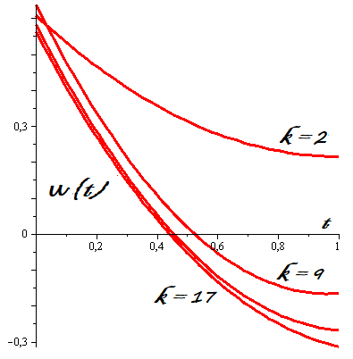
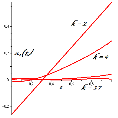
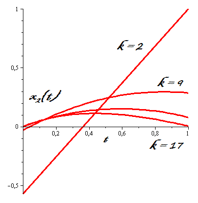
Figure 1: Example 2, control and trajectories on iterations: 2, 9, 13, 17

Example 7.3.

It is required to bring the system

$$\dot{x}_{1}(t)=x_{2}(t)x_{3}(t)+u_{1}(t),$$

$$\dot{x}_{2}(t)=x_{1}(t)x_{3}(t)+u_{2}(t),$$

$$\dot{x}_{3}(t)=x_{1}(t)x_{2}(t)+u_{3}(t)$$

from the initial point $x(0)=(1,0,0)^{\prime}$ to the final state $x(1)=(0,0,0)^{\prime}$ at the moment $T=1$. Herewith, we suppose that the total control consumption is subject to the constraint

$$\int_{0}^{1}|u_{1}(t)|+|u_{2}(t)|+|u_{3}(t)|dt=1.$$

This problem has a practical application to the optimal satellite stabilization and was considered in work Krylov (1968). With the help of the new variable $x_{4}(t)=\displaystyle{\int_{0}^{t}|u_{1}(\tau)|+|u_{2}(\tau)|+|u_{3}(\tau)|d\tau}$ reduce the problem given to problem (5), (6), (8) which is considered in the paper.

Then we have the system

$$\dot{x}_{1}(t)=x_{2}(t)x_{3}(t)+u_{1}(t),$$

$$\dot{x}_{2}(t)=x_{1}(t)x_{3}(t)+u_{2}(t),$$

$$\dot{x}_{3}(t)=x_{1}(t)x_{2}(t)+u_{3}(t),$$

$$\dot{x}_{4}(t)=|u_{1}(t)|+|u_{2}(t)|+|u_{3}(t)|,$$

with no restrictions on the control $u^{*}\in P_{3}[0,T]$ which is aimed at bringing the object from the initial point $x(0)=(1,0,0,0)^{\prime}$ to the final state $x(1)=(0,0,0,1)^{\prime}$ at the moment $T=1$.

The problem given is reduced to an unconstrained minimization of the functional

$$I(x,z,u)=\int_{0}^{1}\big{|}z_{1}(t)-x_{2}(t)x_{3}(t)-u_{1}(t)|dt+\int_{0}^{1}\big{|}z_{2}(t)-x_{1}(t)x_{3}(t)-u_{2}(t)|dt+$$

$$+\int_{0}^{1}\big{|}z_{3}(t)-x_{1}(t)x_{2}(t)-u_{3}(t)|dt+\int_{0}^{1}\big{|}z_{4}(t)-|u_{1}(t)|-|u_{2}(t)|-|u_{3}(t)||dt+$$

$$+\frac{1}{2}\Big{(}1+\int_{0}^{1}z_{1}(t)dt\Big{)}^{2}+\frac{1}{2}\Big{(}\int_{0}^{1}z_{2}(t)dt\Big{)}^{2}+\frac{1}{2}\Big{(}\int_{0}^{1}z_{3}(t)dt\Big{)}^{2}+\frac{1}{2}\Big{(}\int_{0}^{1}z_{4}(t)dt-1\Big{)}^{2}+$$

$$+\frac{1}{2}\sum_{i=1}^{4}\left(x_{i}(t)-x_{i}(0)-\int_{0}^{t}z_{i}(\tau)d\tau\right)^{2}dt.$$

Take $(x_{(1)},z_{(1)},u_{(1)})=(1+t,t,t,t,1,1,1,1,0,0,0)^{\prime}$ as an initial point, then $I(x_{(1)},z_{(1)},u_{(1)})\approx 5.72678$. As the iteration number increased, the discretization rank gradually increased during the solution of the auxiliary problem of finding the direction of quasidifferential descent described in the algorithm and, in the end, the discretization step was equal to $10^{-1}$. At the $58$-th iteration the control $u_{(58)}$ was constructed:

$$u_{1}\approx-2.88657t^{5}+8.96619t^{4}-9.30386t^{3}+2.99867t^{2}+0.10679t-1.03399,$$

$$u_{2}\approx-0.83764t^{5}+0.85068t^{4}+0.43135t^{3}-0.54058t^{2}+0.06933t+0.00945,$$

$$u_{3}\approx 0.13344t-0.01334,\ t\in[0,0.1),\quad 0.03928t^{3}-0.01848t^{2}-0.00194t,\ t\in[0.1,0.6),$$

$$-0.94481t^{3}+2.12646t^{2}-1.55331t+0.36987,\ t\in[0.6,1],$$

with the value of the functional $I(x_{(58)},z_{(58)},u_{(58)})\approx 0.00551$, herewith, $x_{1}(T)\approx 0.01251$, $x_{2}(T)\approx 0.00431$, $x_{3}(T)\approx 0.00431$, $x_{4}(T)\approx 1.0069$. For the convenience of presentation, the Lagrange interpolation polynomial has been given which quite accurately approximates (that is, the interpolation error does not affect the value of the functional and the boundary values) the resulting control.

Take $u_{(58)}$ as an approximation to the control $u^{*}$ sought. In order to verify the result obtained and to find the “true” trajectory, we substitute this control into the system given and integrate it via one of the known numerical methods (here, the Runge-Kutta 4-5-th order method was used). As a result, we have the corresponding trajectory (which is an approximation to the one $x^{*}$ sought) with the values $x_{1}(T)=0.00514$, $x_{2}(T)=0.00204$, $x_{3}(T)=0.00051$, $x_{4}(T)=1.00514$, so we see that the error does not exceed the value $5\times 10^{-3}$. Herewith, $||G(x,z,u)||_{L^{4}_{2}[0,T]\times L^{4}_{2}[0,T]\times L^{3}_{2}[0,T]}=0.00757$.

The computational time was 15 min 32 sec. The pictures illustrate the control and trajectories dynamics during the algorithm realization.

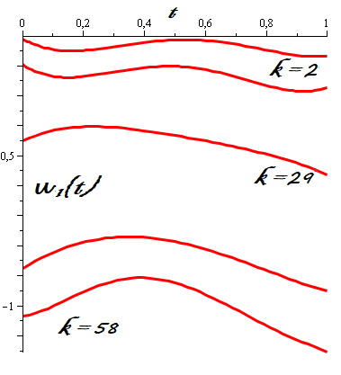
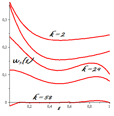
Figure 2: Example 3, control on iterations: 2, 13, 29, 45, 58

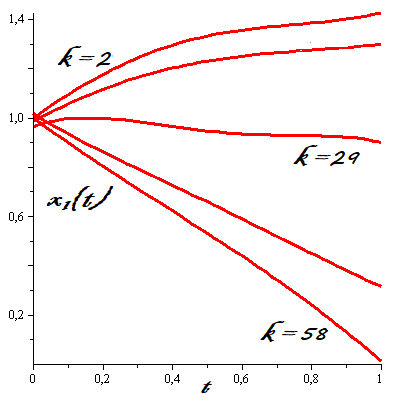
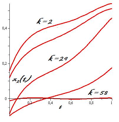
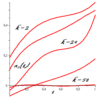
Figure 3: Example 3, trajectories on iterations: 2, 13, 29, 45, 58

Example 7.4.

Consider the system

$$\dot{x}_{1}(t)=x_{2}(t)$$

$$\dot{x}_{2}(t)=u(t)-Px_{2}(t)|x_{2}(t)|-Qx_{2}(t).$$

It is required to find such a control $u^{*}\in U$ which brings this system from the initial point $x(0)=(0,0)^{\prime}$ to the final state $x(48)=(200,0)^{\prime}$ at the moment $T=48$. Herewith, put $\underline{u}=-2/3$, $\overline{u}=2/3$, i. e. we suppose that $-2/3\leq u(t)\leq 2/3$   $\forall t\in[0,48]$. The parameters of the problem are $P=0.78\times 10^{-4}$ and $Q=0.28\times 10^{-3}$. This problem has a practical application to the optimal train motion and was considered in work Outrata (1983). Not that the right-hand side of the system contains a nondifferentiable term. On the other hand, essential assumption of the paper is that only continuous differentiable functions in the right-hand side of the system are allowed (see Outrata (1983), Par. 2, Assumption. (ii)). So the paper Outrata (1983) method presumably can not be implemented on those iterations when the nondifferentiability in the system right-hand side occurs (as for example, on the first iteration in our case since the initial approximation point $z_{(1)}=(0,0,0)^{\prime}$ is taken (see the next paragraph)). (However, the paper Outrata (1983) method eventually succeeded in this example, since $x_{2}^{*}(t)>0$ for all $t\in(0,48)$.)

In fact, in paper Outrata (1983) a more complicated (if we “ignore” the fact that the right-hand side of the system is formally nondifferentiable) problem is considered with some phase constraints and the functional

$$\int_{0}^{48}x_{2}(t)\max\{u(t),0\}dt$$

to be minimized. The paper gives neither the optimal control nor the resulting cost value obtained; the rough estimate of the “characteristic” segments (where $u(t)>0$) given in Fig. 1, Par. 5.1 of Outrata (1983) (we duplicate this picture as well) shows that the functional optimal value exceeds the magnitude $13.3$.

We consider a simplified problem; however, let us try to obtain this value of the functional via the new variable $x_{3}(t)=\displaystyle{\int_{0}^{t}x_{2}(\tau)\max\{u(\tau),0\}d\tau}$ and explore the system with the additional equation

$$\dot{x}_{3}(t)=x_{2}(t)\max\{u(t),0\}$$

and with the boundary conditions $x(0)=(0,0,0)^{\prime}$ and $x(48)=(200,0,13.3)^{\prime}$ (and without any phase constraints).

The problem given is reduced to an unconstrained minimization of the functional

$$I(z,u)=\int_{0}^{48}\big{|}z_{2}(t)-u(t)+Pz_{1}(t)|z_{1}(t)|+Qz_{1}(t)\big{|}dt+\int_{0}^{48}\big{|}z_{3}(t)-z_{1}(t)\max\{u(t),0\}\big{|}dt$$

$$+\frac{1}{2}\Big{(}\int_{0}^{48}z_{1}(t)dt-200\Big{)}^{2}+\frac{1}{2}\Big{(}\int_{0}^{48}z_{2}(t)dt\Big{)}^{2}+\frac{1}{2}\Big{(}\int_{0}^{48}z_{3}(t)dt-13.3\Big{)}^{2}$$

$$+\int_{0}^{48}\max\{-2/3-u(t),0\}dt+\int_{0}^{48}\max\{{u}(t)-2/3,0\}dt+$$

$$+\frac{1}{2}\int_{0}^{48}\Big{(}z_{1}(t)-\int_{0}^{t}z_{2}(\tau)d\tau\Big{)}^{2}dt.$$

The functional is slightly simplified beforehand using the fact that $x_{2}(t)=z_{1}(t)$, also put $\displaystyle{x_{1}(t)=\int_{0}^{t}z_{1}(\tau)d\tau}$, $\displaystyle{x_{3}(t)=\int_{0}^{t}z_{3}(\tau)d\tau}$, $t\in[0,48]$, throughout iterations.

Take $(z_{(1)},u_{(1)})=(0,0,0,0)^{\prime}$ as an initial point, then $I(z_{(1)},u_{(1)})=2\times 10^{4}$. As the iteration number increased, the discretization rank gradually increased during the solution of the auxiliary problem of finding the direction of the quasidifferential descent described in the algorithm and, in the end, the discretization step was equal to $2\times 10^{-1}$ on the intervals $[0,9]$ and $[40,48]$ and equal to $3.875$ on the interval $[9,40]$ (it was reasonable to use a nonuniform (and such a rough in the middle interval) splitting here due to the qualitative different “behavior” of the trajectories on these intervals). At the $216$-th iteration the control $u_{(216)}$ was constructed:

$$u\approx 0.666667,\ t\in[0,4.383),$$

$$0.09896701901t-0.01727775583t^{2}+0.5648118155,\ t\in[4.383,9),$$

$$-3.398320586\times 10^{-10}\,t^{6}+6.378460924\times 10^{-8}\,t^{5}-0.000003933576898t^{4}+$$

$$+0.00010132955t^{3}-0.00075674151t^{2}-0.01180182196t+0.1719284027,\ t\in[9,40),$$

$$-0.03302426450t^{3}+4.273406929t^{2}-184.2002092t+2644.154001,\ t\in[40,42),$$

$$-0.666667,\ t\in[42,48],$$

with the value of the functional $I(z_{(216)},u_{(216)})\approx 0.00124$, herewith $x_{1}(T)\approx 200.001$, $x_{2}(T)\approx 0.00521$, $x_{3}(T)\approx 13.30413$. For the convenience of presentation, the Lagrange interpolation polynomial has been given which quite accurately approximates (that is, the interpolation error does not affect the value of the functional and the boundary values) the resulting control.

Note that during the method implementation the control was obtained bringing the trajectory from an initial position given to the final point satisfying the right endpoint constraint with the satisfactory accuracy (and delivering a rather small value to the functional minimized as well); however, this control itself violated its own restrictions by the value $2\times 10^{-2}$ — $4\times 10^{-2}$ at the beginning and the end of the time interval (see the control dynamics in the picture). Since the exact satisfaction of the restrictions on control is important for applications, on several last iterations it was decided to improve the accuracy via multiplying the $6$-th and the $7$-th summands of the functional by a large factor (of order $10^{2}$) and minimizing this modified functional during the last iterations.

Take $u_{(216)}$ as an approximation to the control $u^{*}$ sought. In order to verify the result obtained and to find the “true” trajectory, we substitute this control into the system given and integrate it via one of the known numerical methods (here, the Runge-Kutta 4-5-th order method was used). As a result, we have the corresponding trajectory (which is an approximation to the one $x^{*}$ sought) with the values $x_{1}(T)\approx 200.00214$, $x_{2}(T)\approx 0.00297$, $x_{3}(T)\approx 13.3054$, so we see that the error does not exceed the value $5\times 10^{-3}$. Herewith, $||G(z,u)||_{L^{3}_{2}[0,T]\times L^{1}_{2}[0,T]}=0.00299$.

The computational time was 102 min 43 sec. The pictures illustrate the control and trajectories dynamics during the algorithm realization. For convenience also the resulting control and trajectories are depicted.

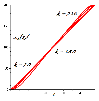
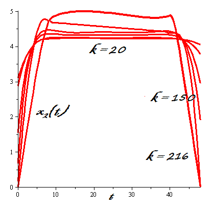
Figure 4: Example 4, control and trajectories on iterations: 20, 50, 100, 150, 175, 200, 216

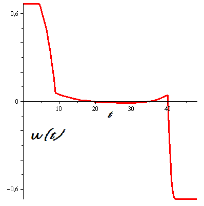
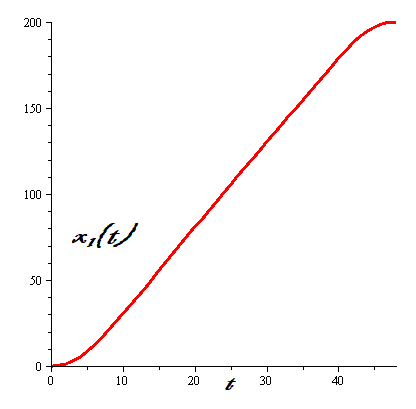
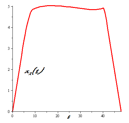
Figure 5: Example 4, the resulting control and trajectories

8 Discussion

As already noted, the main advantage of the method proposed is of theoretical nature: it is original as it is qualitatively different from existing methods based on the direct discretization of the initial problem. Besides, the method preserves attractive geometrical interpretation of quasidifferentials (see Example 7.1 and Ch. V, Par. 3 in book Demyanov & Rubinov (1977) for more examples with geometrical illustration in the finite-dimensional case).

It also has some practical advantages. The following four paragraphs give examples of some specific problems demonstrating these advantages. In order to simplify the presentation and just to get essence we give examples of some problems of calculus of variations and an example of one simplest control problem only in a smooth case.

Consider the problem of minimizing the functional

$$J(x,z)=\int_{0}^{1}z^{4}(t)/48+z^{2}(t)+x^{2}(t)-6x(t)\,dt$$

under the constraints

$$x(0)=1,\quad x(1)=0,\quad\int_{0}^{1}x(t)\,dt=2/3.$$

In this example the steepest descent method appeared to be very effective. On the contrary: in order to construct approximations by the Ritz-Galerkin method, a lot of calculations are required and it is also necessary to solve essentially non-linear systems with parameters.

In a problem of minimizing the the functional

$$J(z)=\int_{0}^{10}z^{2}(t)-x^{2}(t)\,dt$$

under the constraints

$$x(0)=0,\quad x(10)=0$$

both the Euler equation and the Ritz-Galerkin method give a trajectory delivering neither a strong nor a weak minimum. The steepest descent method “points” to the fact that there is no solution in this problem: the one-dimensional minimization problem has no bounded solution.

Minimize the functional

$$J(z)=\int_{0}^{2}z^{3}(t)\,dt$$

under the constraints

$$x(0)=0,\quad x(2)=4.$$

This example illustrates that the steepest descent method “points” to the fact that, on a solution obtained, the functional reaches a weak minimum rather than a strong one, while both the Euler equation and the Ritz-Galerkin method give only a trajectory delivering a weak minimum.

All the details have been omitted for brevity. One can find a detailed description of these problems and more interesting examples as well as justification of the statements posed in the original papers Demyanov & Tamasyan (2011), Demyanov & Tamasyan (2010). Note also that a method used in these papers is slightly different from the one presented but it preserves its many properties, so the comparative analysis is correct.

Consider the system

$$\dot{x}(t)=-x(t)+u(t)$$

on the time interval $[0,2]$. It is required to find a control $u^{*}\in P_{1}[0,T]$ such that the corresponding trajectory satisfies the boundary conditions

$$x(0)=x(2)=0.$$

Apply direct discretization to this system via the formula

$$x(i+1)-x(i)=\frac{1}{N}(-x(i)+u(i))$$

where $i=\overline{0,19}$ and the discretization rank $N=20$. If we use the initial condition $x_{0}=x(0)=0$ and calculate $x_{20}=x(2)$ as an explicit function of the variables $u_{i}$, $i=\overline{0,19}$, we will obtain

$$x_{20}(u)\approx 0.01886768013\,u_{0}+0.01986071592\,u_{1}+0.02090601676\,u_{2}+\,0.0220063334\,u_{3}+$$

$$+0.02316456151\,u_{4}+0.02438374896\,u_{5}+0.02566710416\,u_{6}+0.02701800438\,u_{7}+$$

$$+0.02844000461\,u_{8}+0.02993684696\,u_{9}+0.03151247049\,u_{10}+0.03317102156\,u_{11}+$$

$$+0.03491686480\,u_{12}+0.03675459453\,u_{13}+0.03868904688\,u_{14}+0.04072531250\,u_{15}+$$

$$+0.04286875000\,u_{16}+0.045125\,u_{17}+0.0475\,u_{18}+0.05\,u_{19}.$$

So in order to get the required finite position, one has to solve the equation $x_{20}(u)=0$ with respect to the variables $u_{i}$, $i=\overline{0,19}$. In other words, it is required to minimize the functional $|x_{20}(u)|$. Take the initial point $u_{(0)}$ with the following coordinates: $u_{2i}=10$, $i=\overline{0,9}$, $u_{2i+1}=-10$, $i=\overline{0,8}$, $u_{19}\approx-6.7101842175$ (see the picture). Note that $x_{20}(u_{(0)})=0$, so the point $u_{(0)}$ delivers a global minimum to the functional $|x_{20}(u)|$ (i. e. the point $u_{(0)}$ solves the discretized problem). However, if we substitute this control $u_{(0)}$ into the original system, we will get the corresponding trajectory $x_{(0)}(t)$ with the finite value $x(2)\approx-0.1189349683$.

Now try to solve this problem via the method of the paper, i. e. minimize the functional

$$I(x,z,u)=\frac{1}{2}\int_{0}^{2}\left(z(t)+x(t)-u(t)\right)^{2}dt+\frac{1}{2}\int_{0}^{2}\left(x(t)-\int_{0}^{t}z(\tau)d\tau\right)^{2}dt+\frac{1}{2}\left(\int_{0}^{2}z(t)dt\right)^{2}$$

(for simplicity of presentation we have taken a square-function instead of the abs-function as the integrand in the first summand). Take the same point $(x_{(0)},z_{(0)},u_{(0)})^{\prime}$ (where $z_{(0)}=\dot{x}_{(0)}$) as an initial approximation. One can check that on the first iteration we will get such a control that the corresponding trajectory takes the finite value $|x(2)|<0.11894$ (i. e. “better” than that one obtained via discretization method).

In fact, applying the method to this example one can get a solution with any given accuracy. This is due the fact that the Gateaux gradient in this case is as follows:

$$\nabla I(x,z,u,t)=\begin{pmatrix}\big{(}z(t)+x(t)-u(t)\big{)}+\displaystyle{\left(x(t)-\int_{0}^{t}z(\tau)d\tau\right)}\\ \big{(}z(t)+x(t)-u(t)\big{)}-\displaystyle{\left(\int_{t}^{2}\Big{(}x(\tau)-\int_{0}^{\tau}z(s)ds\Big{)}d\tau\right)}+\int_{0}^{2}z(t)\,dt\\ -\big{(}z(t)+x(t)-u(t)\big{)}\end{pmatrix}.$$

Hence, the stopping criteria (that is $||\nabla I(x^{*},z^{*},u^{*})||_{L_{2}^{1}[0,2]\times L_{2}^{1}[0,2]\times L_{2}^{1}[0,2]}=0$ in this case) may be only fulfilled (with some accuracy) when the third component of the gradient vanishes. This fact implies that the second summand in the first component vanishes. This fact finally implies that the third summand in the second component vanishes. Thus, we see that there are no local minima of the functional considered, so the method of the paper will lead to the desired solution (with any given accuracy). Roughly speaking, the method proposed “analyzes” the “behavior” of the whole trajectory, rather than only its points considered at some discrete moments of time.

Although in this example the initial control is chosen in a special way, one can easily check that there is a “huge” number of other controls with the same properties (i. e. delivering a global minimum to the functional $|x_{T}(u)|$ but giving an error to the right endpoint value). Both increasing the time moment $T$ and adding some kind of nonsmoothness in the right-hand side of the system given (for example taking the function $-|x(t)|$ instead of $-x(t)$ now) will only increase this “huge” number. Of course, while increasing discretization rank, one can decrease the error on the right endpoint. On the other hand, even the discretization rank taken seems to be not very high for control problems solved via discretization or a “control parametrization” technique (see, e. g. Teo & Goh & Wong (1991)). Besides, for any discretization rank taken the initial control may be chosen in such a way that it will deliver the global minimum to the functional minimized (i. e. $x_{T}(u_{(0)})=0$) but give an arbitrary large error to the right endpoint value.

As noted, only the smooth case in the examples given is considered for simplicity. A nonsmooth case may lead to even more difficulties: for example, in the control problem presented any kind of nondifferentiability in the right-hand side will significantly increase the number of “local” minima with direct discretization used.

List also some secondary advantages of the method proposed:

1) although large discretization rank gives a good approximation to the original problem, the choice of the appropriate discretization rank is not straightforward;

2) in many cases the quasidifferential descent method rapidly demonstrates the structure of the desired solution, although then the convergence to this solution may be very slow;

3) any integral restriction (for example, $||u(t)||^{2}_{L_{2}^{m}[0,T]}\leq C$, $C\in R$ given) will generate a complicated constraint with a large number of variables (equal to the discretization rank) after direct discretization is applied to the problem; on the contrary: the integral restriction is very natural for the variational statement of the problem solved and it is easy to add a corresponding summand to the functional $I(x,z,u)$ in order to take this restriction into account.

The main disadvantage of the method presented in this paper reduces to the computational effort: the number of iterations may be very large and the accuracy obtained is often not very high (although mostly appropriate for applications). Despite the comparative disadvantages listed, in many problems direct discretization is more preferable than the method proposed, both in terms of the number of iterations implemented and of the accuracy achieved. The current and future research work is devoted to implementing some modifications and simplicities aimed at increasing the method computational efficiency.

9 Conclusion

The paper is devoted to developing a direct “continuous” method for a nonsmooth control problem. The problem of bringing a system with a nondifferentiable (but only quasidifferentiable) right-hand side from one point to another is considered. The admissible controls are those from the space of piecewise continuous vector-functions which belong to some parallelepiped at each moment of time. The problem of finding the steepest (the quasidifferential) descent direction was solved and the quasidifferential descent method was applied to some illustrative examples. The method is original and is qualitatively different from the existing methods as most of them are based on direct discretization of the original problem. The main and new idea implemented is to consider phase trajectory and its derivative as independent variables and to take the natural relation between these variables into account via penalty function of a special form. This idea gives possibility to calculate the quasidifferential of the minimized functional and eventually to obtain the steepest descent direction. As computational effort of the method proposed is rather high, the goal of the future research is to improve computational efficiency. Another goal is to applicate the main ideas presented to other control problems.

Appendix

With the help of quasidifferential calculus rules (Demyanov & Rubinov (1977), Ch. III, Par. 2) at each $i\in\{1,\dots,n\}$, $j\in\{1,\dots,m\}$ and at each $t\in[0,T]$ calculate the quasidifferentials below.

$$\mathcal{D}\,\big{|}z_{i}(t)-f_{i}(x(t),u(t),t)\big{|}=\left[\left(\begin{array}[]{c}0\\ \vdots\\ 0\\ 1\\ 0\\ \vdots\\ 0\end{array}\right)-\overline{\partial}f_{i}(x,u,t),\ -\underline{\partial}f_{i}(x,u,t)\right],$$

if $z_{i}-f_{i}(x,u,t)>0$. Here $1$ is on the $(n+i)$-th place.

$$\mathcal{D}\,\big{|}z_{i}(t)-f_{i}(x(t),u(t),t)\big{|}=\left[\left(\begin{array}[]{c}0\\ \vdots\\ 0\\ -1\\ 0\\ \vdots\\ 0\end{array}\right)+\underline{\partial}f_{i}(x,u,t),\ \overline{\partial}f_{i}(x,u,t)\right],$$

if $z_{i}-f_{i}(x,u,t)<0$. Here $-1$ is on the $(n+i)$-th place.

$$\mathcal{D}\,\big{|}z_{i}(t)-f_{i}(x(t),u(t),t)\big{|}=$$

$$=\left[\mathrm{co}\left\{\left(\begin{array}[]{c}0\\ \vdots\\ 0\\ 1\\ 0\\ \vdots\\ 0\end{array}\right)-2\,\overline{\partial}f_{i}(x,u,t),\,\left(\begin{array}[]{c}0\\ \vdots\\ 0\\ -1\\ 0\\ \vdots\\ 0\end{array}\right)+2\,\underline{\partial}f_{i}(x,u,t)\right\},\ -\underline{\partial}f_{i}(x,u,t)+\overline{\partial}f_{i}(x,u,t)\right],$$

if $z_{i}-f_{i}(x,u,t)=0$. Here $1$ and $-1$ are on the $(n+i)$-th place.

$$\mathcal{D}\max\big{\{}u_{j}(t)-\overline{u}_{j},0\big{\}}=\left[\left(\begin{array}[]{c}0\\ \vdots\\ 0\\ 1\\ 0\\ \vdots\\ 0\end{array}\right),\ 0_{m}\right],$$

if $u_{j}-\overline{u}_{j}>0$. Here $1$ is on the $j$-th place.

$$\mathcal{D}\max\big{\{}u_{j}(t)-\overline{u}_{j},0\big{\}}=\left[0_{m},\ 0_{m}\right],$$

if $u_{j}-\overline{u}_{j}<0$.

$$\mathcal{D}\max\big{\{}u_{j}(t)-\overline{u}_{j},0\big{\}}=\left[\mathrm{co}\left\{\left(\begin{array}[]{c}0\\ \vdots\\ 0\\ 1\\ 0\\ \vdots\\ 0\end{array}\right),\,0_{m}\right\},\ 0_{m}\right],$$

if $u_{j}-\overline{u}_{j}=0$. Here $1$ is on the $j$-th place.

$$\mathcal{D}\max\big{\{}\underline{u}_{j}-u_{j}(t),0\big{\}}=\left[\left(\begin{array}[]{c}0\\ \vdots\\ 0\\ -1\\ 0\\ \vdots\\ 0\end{array}\right),\ 0_{m}\right],$$

if $\underline{u}_{j}-{u}_{j}(t)>0$. Here $-1$ is on the $j$-th place.

$$\mathcal{D}\max\big{\{}\underline{u}_{j}-u_{j}(t),0\big{\}}=\left[0_{m},\ 0_{m}\right],$$

if $\underline{u}_{j}-{u}_{j}(t)<0$.

$$\mathcal{D}\max\big{\{}\underline{u}_{j}-u_{j}(t),0\big{\}}=\left[\mathrm{co}\left\{\left(\begin{array}[]{c}0\\ \vdots\\ 0\\ -1\\ 0\\ \vdots\\ 0\end{array}\right),\,0_{m}\right\},\ 0_{m}\right],$$

if $\underline{u}_{j}-{u}_{j}(t)=0$. Here $-1$ is on the $j$-th place.

In the previous paragraph formulas the subdifferentials $\underline{\partial}f_{i}(x,u,t)$ and the superdifferentials $\overline{\partial}f_{i}(x,u,t)$, $i=\overline{1,n}$, are calculated via quasidifferential calculus apparatus as well. Book Demyanov & Rubinov (1977) (see Ch. III, Par. 2 there) contains a detailed description of these rules for a rich class of functions. Let us give just some of these rules which were used in the formulas of the previous paragraph. Let $\xi\in R^{l}$. If the function $\varphi(\xi)$ is quasidifferentiable at the point $\xi_{0}\in R^{l}$ and $\lambda$ is some number, then we have

$$\lambda\,\mathcal{D}\varphi(\xi_{0})=[\lambda\,\underline{\partial}\varphi(\xi_{0}),\lambda\,\overline{\partial}\varphi(\xi_{0})],\quad\text{if}\ \lambda\geqslant 0,$$

$$\lambda\,\mathcal{D}\varphi(\xi_{0})=[\lambda\,\overline{\partial}\varphi(\xi_{0}),\lambda\,\underline{\partial}\varphi(\xi_{0})],\quad\text{if}\ \lambda<0.$$

If the functions $\varphi_{k}(\xi)$, $k=\overline{1,r}$, are quasidifferentiable at the point $\xi_{0}\in R^{l}$, then the quasidifferntial of the function $\varphi(\xi)=\max_{k=\overline{1,r}}\varphi_{k}(\xi)$ at this point is calculated by the formula

$$\mathcal{D}\varphi(\xi_{0})=[\underline{\partial}\varphi(\xi_{0}),\overline{\partial}\varphi(\xi_{0})],$$

$$\underline{\partial}\varphi(\xi_{0})=\mathrm{co}\Big{\{}\underline{\partial}\varphi_{k}(\xi_{0})-\sum_{i\in P(\xi_{0}),\ i\neq k}\overline{\partial}\varphi_{i}(\xi_{0}),\ k\in P(\xi_{0})\Big{\}},$$

$$\overline{\partial}\varphi(\xi_{0})=\sum_{i\in P(\xi_{0})}\overline{\partial}\varphi_{i}(\xi_{0}),$$

$$P(\xi_{0})=\{k\in\{1,\dots,r\}\ |\ \varphi_{k}(\xi_{0})=\varphi(\xi_{0})\}.$$

If the functions $\varphi_{k}(\xi)$, $k=\overline{1,r}$, are quasidifferentiable at the point $\xi_{0}\in R^{l}$, then the quasidifferntial of the function $\varphi(\xi)=\min_{k=\overline{1,r}}\varphi_{k}(\xi)$ at this point is calculated by the following formula

$$\mathcal{D}\varphi(\xi_{0})=[\underline{\partial}\varphi(\xi_{0}),\overline{\partial}\varphi(\xi_{0})],$$

$$\underline{\partial}\varphi(\xi_{0})=\sum_{j\in Q(\xi_{0})}\underline{\partial}\varphi_{j}(\xi_{0}),$$

$$\overline{\partial}\varphi(\xi_{0})=\mathrm{co}\Big{\{}\overline{\partial}\varphi_{k}(\xi_{0})-\sum_{j\in Q(\xi_{0}),\ j\neq k}\underline{\partial}\varphi_{j}(\xi_{0}),\ k\in Q(\xi_{0})\Big{\}},$$

$$Q(\xi_{0})=\{k\in\{1,\dots,r\}\ |\ \varphi_{k}(\xi_{0})=\varphi(\xi_{0})\}.$$

Note also that if the function $\varphi(\xi)$ is subdifferentiable at the point $\xi_{0}\in R^{l}$, then its quasidifferential at this point may be represented in the form

$$\mathcal{D}\varphi(\xi_{0})=[\underline{\partial}\varphi(\xi_{0}),0_{l}],$$

and if the function $\varphi(\xi)$ is superdifferentiable at the point $\xi_{0}\in R^{l}$, then its quasidifferential at this point may be represented in the form

$$\mathcal{D}\varphi(\xi_{0})=[0_{l},\overline{\partial}\varphi(\xi_{0})].$$

These two formulas can be taken as definitions of a subdifferentiable and a superdifferentiable function respectively. If the function $\varphi(\xi)$ is differentiable at the point $\xi_{0}\in R^{l}$, then its quasidifferential may be represented in the forms

$$\mathcal{D}\varphi(\xi_{0})=[\varphi^{\prime}(\xi_{0}),0_{l}]\ \mathrm{or}\ \mathcal{D}\varphi(\xi_{0})=[0_{l},\varphi^{\prime}(\xi_{0})],$$

where $\varphi^{\prime}(\xi_{0})$ is a gradient of the function $\varphi(\xi)$ at the point $\xi_{0}$. The latter fact indicates that there is not the only way to construct quasidifferential. We also note that the subdifferential (the superdifferential) of the finite sum of quasidifferentiable functions is a sum of subdifferentials (superdifferentials) of the summands, i. e. if the functions $\varphi_{k}(\xi)$, $k=\overline{1,r}$, are quasidifferentiable at the point $\xi_{0}\in R^{l}$, then the quasidifferential of the function $\varphi(\xi)=\sum_{k=1}^{r}\varphi_{k}(\xi)$ at this point is calculated by the formula

$$\mathcal{D}\varphi(\xi_{0})=\left[\sum_{k=1}^{r}\underline{\partial}\varphi_{k}(\xi_{0}),\sum_{k=1}^{r}\overline{\partial}\varphi_{k}(\xi_{0})\right].$$

Via the rules given and formulas (12) and (13) we find the quasidifferentials $\mathcal{D}I_{1}(x,z,u)$ and $\mathcal{D}I_{3}(u)$.

References

- Demyanov & Rubinov (1977) Demyanov V. F., Rubinov A. M. Basics of nonsmooth analysis and quasidifferential calculus. 1990. Moscow: Nauka. (in Russian)