DefakeHop++: An Enhanced Lightweight Deepfake Detector

Hong-Shuo Chen Shuowen Hu Suya You C.-C. Jay Kuo University of Southern California, Los Angeles, California, USA Army Research Laboratory, Adelphi, Maryland, USA

Abstract

On the basis of DefakeHop, an enhanced lightweight Deepfake detector called DefakeHop++ is proposed in this work. The improvements lie in two areas. First, DefakeHop examines three facial regions (i.e., two eyes and mouth) while DefakeHop++ includes eight more landmarks for broader coverage. Second, for discriminant features selection, DefakeHop uses an unsupervised approach while DefakeHop++ adopts a more effective approach with supervision, called the Discriminant Feature Test (DFT). In DefakeHop++, rich spatial and spectral features are first derived from facial regions and landmarks automatically. Then, DFT is used to select a subset of discriminant features for classifier training. As compared with MobileNet v3 (a lightweight CNN model of 1.5M parameters targeting at mobile applications), DefakeHop++ has a model of 238K parameters, which is 16% of MobileNet v3. Furthermore, DefakeHop++ outperforms MobileNet v3 in Deepfake image detection performance in a weakly-supervised setting.

keywords:

Deepfake detection, green learning, green AI, weakly-supervised learning.

\articledatabox

ISSN 2161-1823; DOI 10.1561/103.00000003
© Hong-Shuo Chen

1 Introduction

It is common to see fake videos appearing in social media platforms nowadays due to the popularity of Deepfake techniques. Several mobile apps can help people create fake contents without any special editing skill. Generally speaking, deepfake programs can change the identity of one person in real videos to another realistically and easily. The number of Deepfake videos surges rapidly in recent years. Fake videos may result in serious damages to our society since people can be fooled by them delivered by the Internet and some misinformation may make the public panic and anxious. To address this emerging threat, it is essential to develop lightweight Deepfake detectors that can be deployed in mobile phones.

With the fast growing Generative Adversarial Network (GAN) technology, image forgery techniques keep evolving in recent years. They are effective in reducing manipulation traces detectable by human eyes. It becomes very challenging to distinguish Deepfake images from real ones with human eyes against new generations of Deepfake technologies. Furthermore, adding different kinds of perturbation (e.g., blur, noise and compression) can hurt the detection performance of Deepfake detectors since manipulation traces are mixed with perturbations. A robust Deepfake detector should be able to tell the differernces between real images and fake images generated by the GAN techniques although both of them experience such modifications.

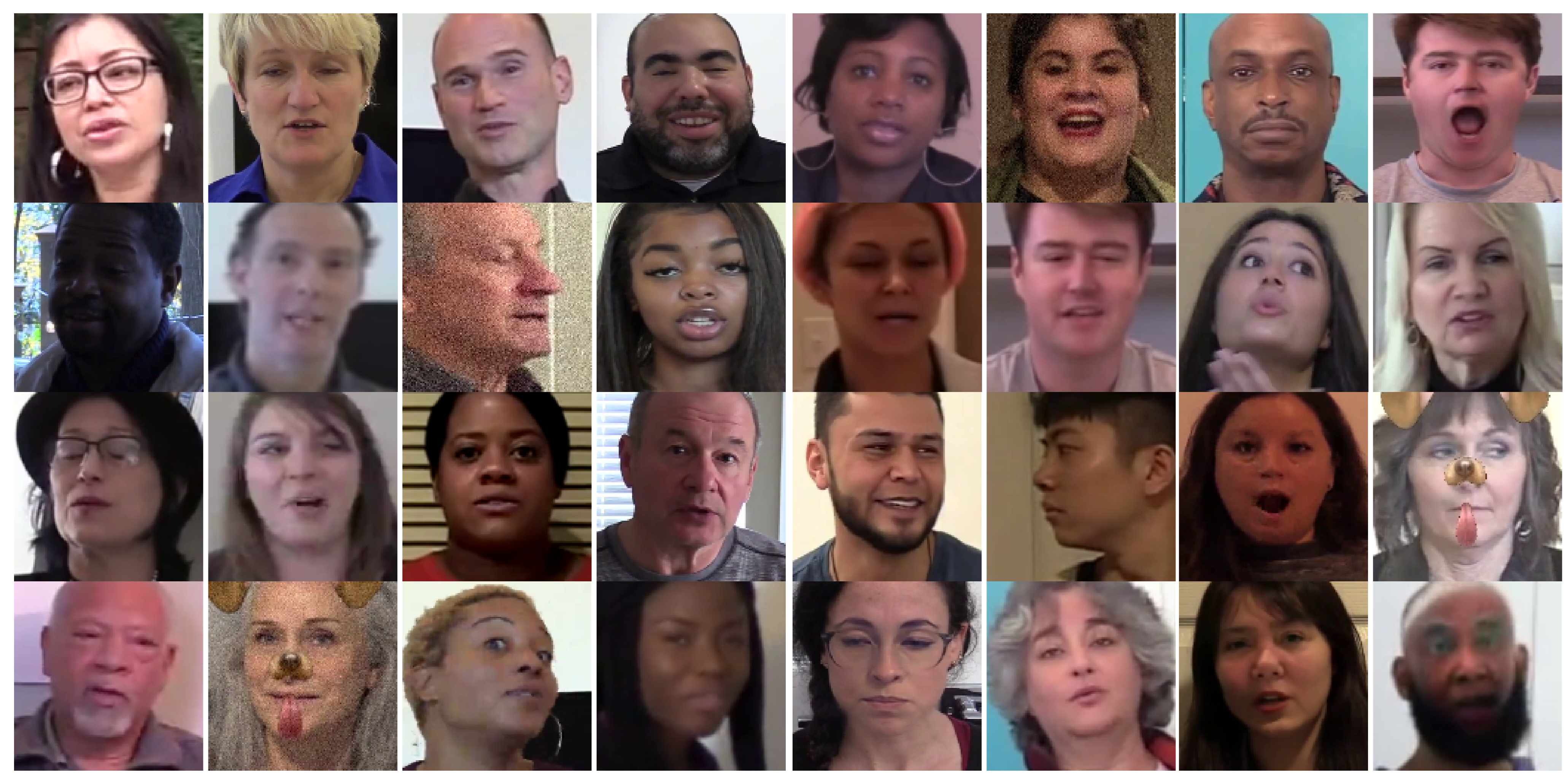
There have been three generations of fake video datasets created for the research and development purpose. They demonstrate the evolution of Deepfake techniques. The UADFV dataset (li2018exposing) belongs to the first generate. It has only 50 video clips generated by one Deepfake method. Its real and fake videos can be easily detected by humans. FaceForensics++ (rossler2019faceforensics++) and Celeb-DF-v2 (li2020celeb) are examples of the second generation. They contain more video clips with more identities. It is difficult for humans to distinguish real and fake faces for them. DFDC (dolhansky2020deepfake) is the third generation dataset. It contains more than 100K fake videos which are generated by 8 Deepfake techniques and perturbed by 19 kinds of distortions. The size of the third generation dataset is very large. It is designed to test the performance of various Deepfake detectors in an environment close to real world applications.

Refer to caption — Figure 1: Visualization of real and fake faces extracted from the third generation DFDC dataset (dolhansky2020deepfake). The left and right four columns depict real and fake faces, respectively. Eight Deepfake techniques are used to generate fake videos. Furthermore, 19 perturbations are added to real and fake videos. Exemplary perturbations include compression, additive noise, blur, change of brightness, contrast and resolution, and overlay with flower and dog patterns, random faces and images. A good Deepfake detector should be able to distinguish real and fake videos with or without perturbation.

State-of-the-art Deepfake detectors usually use the deep neural networks (DNNs) to solve the Deepfake detection problem. Although they offer high detection performance, their model sizes are so large that they cannot be deployed on mobile phones. For example, the winning team of the DFDC contest (seferbekov2020dfdc) used seven pre-trained EfficientNets that contain 432 million parameters. In this research, our goal is to develop a lightweight model with its size less than 256K. For a machine learning model with size less than 256K, it can be run in any terminal device with a limited amount of memory such as Raspberry Pi.

A lightweight Deepfake detector called DefakeHop was developed in (chen2021defakehop). An enhanced version of DefakeHop, called DefakeHop++, is proposed in this work. The improvements lie in two areas. First, DefakeHop examines three facial regions (i.e., two eyes and mouth) only. DefakeHop++ includes eight more landmark regions to offer more information of human faces. Second, DefakeHop uses an unsupervised energy criterion to select discriminant features. It does not exploit the correlation between features and labels. DefakeHop++ adopts a supervised tool, called the Discriminant Feature Test (DFT), in feature selection. The latter is more effective than the former due to supervision. In DefakeHop++, spatial and spectral features from multiple facial regions and landmarks are generated automatically and, then, DFT is used to select a subset of discriminant features to train a classifier. As compared with MobileNet v3, which a lightweight CNN model of 1.5M parameters targeting at mobile applications, DefakeHop++ has an even smaller model size of 238K parameters (i.e., 16% of MibileNet v3). In terms of Deepfake image detection performance, DefakeHop++ outperforms MobileNet v3 without data augmentation and leverage of pre-trained models.

The rest of the paper is organized as follows. Related work is reviewed in Sec. 2. DefakeHop++ is described in detail in Sec. 3. Experimental results are shown in Sec. 4. Finally, concluding remarks are given in Sec. 5.

2 Review of Related Work

Deepfake Detection. Most state-of-the-art Deepfake detection methods use DNNs to extract features from faces. Their models are trained with heavy augmentation (e.g., deleting part of faces) to increase the performance. Despite the high performance of these models, their model sizes are usually very large. They have to be pre-trained by other datasets in order to converge. Several examples are given below. The model of the winning team of the DFDC Kaggle challenges (seferbekov2020dfdc) has 432M parameters. Heo et al. (heo2021deepfake) improved this model by concatenating it with a Vision Transformer(VIT), which has 86M parameters. Zhao et al. (zhao2021multi) proposed a model that exploits multiple spatial attention heads to learn various local parts of a face and the textural enhancement block to learn subtle facial artifacts. To reduce the model size and improve the efficiency, Sun et al. (sun2021improving) proposed a robust method based on the change of landmark positions in a video. These landmarks are calibrated by the neighbor frames. Afterwards, a two-stream RNN is trained to learn the temporal information of the landmark position. Since they did not consider the image information and only consider the position information, the model size is 0.18M which is relatively small. Tran et al. (tran2021high) applied MobileNet to different facial regions and InceptionV3 to the entire faces. Although this model is smaller, it still demands 26M parameters.

DefakeHop. To address the challenge of the need of huge model sizes and training data, a new machine learning paradigm called green learning has been developed in the last six years (kuo2016understanding; kuo2019interpretable; chen2019pixelhop; chen2020pixelhop++). Its main goal is to reduce the model size and training time while keep high performance. Green learning has been applied to different applications, e.g., (liu2021voxelhop; monajatipoor2021berthop; zhang2021anomalyhop; rouhsedaghat2021low; rouhsedaghat2021facehop; zhang2020unsupervised; kadam2021r; zhang2020pointhop; zhang2020pointhop++). Based on green learning, DefakeHop was developed in (chen2021defakehop) for the Deepfake detection task. It first extracts a large number of features from three facial regions using PixelHop++ (chen2019pixelhop) and then refines them using feature distillation modules. Finally, it feeds distilled features to the XGBboost classifier (chen2016xgboost). The DefakeHop model has only 42.8K parameters, yet it outperforms many DNN solutions in detection accuracy against the first and second generataion Deepfake datasets. Recently, DefakeHop has been used to detect fake satellite images in (chen2021geo).

3 DefakeHop++

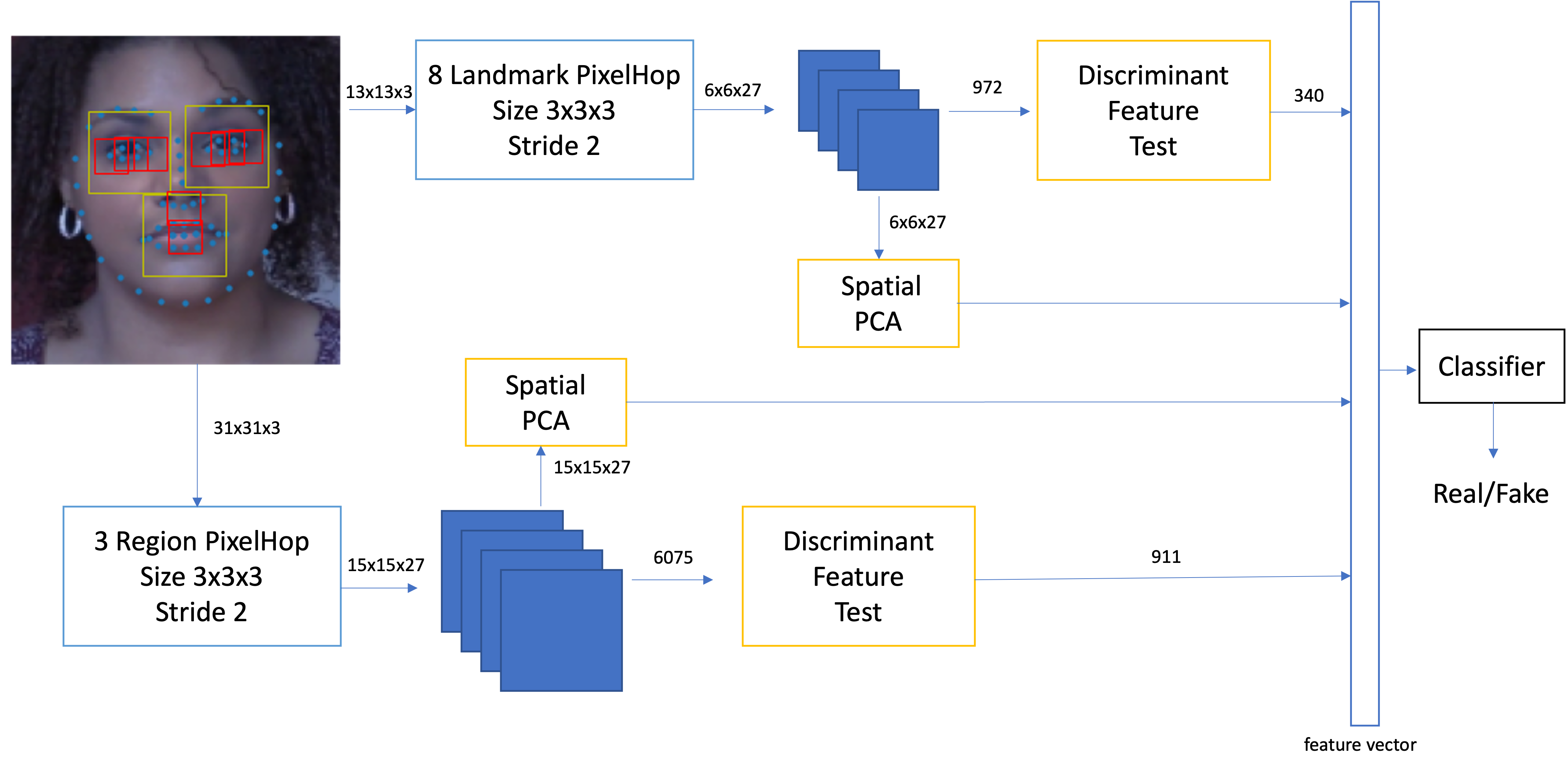
DefakeHop++ is an improved version of DefakeHop. An overview of the DefakeHop++ system is shown in Fig. 2. Facial blocks of two sizes are first extracted from frames in a video sequence in the pre-processing step. These blocks are then passed to DefakeHop++ for processing. DefakeHop++ consists of four modules: 1) one-stage PixelHop, 2) spatial PCA, 3) discriminant feature test (DFT), and 4) Classifier. The pre-processing step and the four modules are elaborated below.

3.1 Pre-processing Step

Frames are extracted from video sequences. For training videos, we extract three frames per second. Since the video length is typically around 10 seconds, we obtain around 30 frames per video. On the other hand, the length and the frame number per second (FPS) are not fixed in test videos. We uniformly sample 100 frames from each test video.

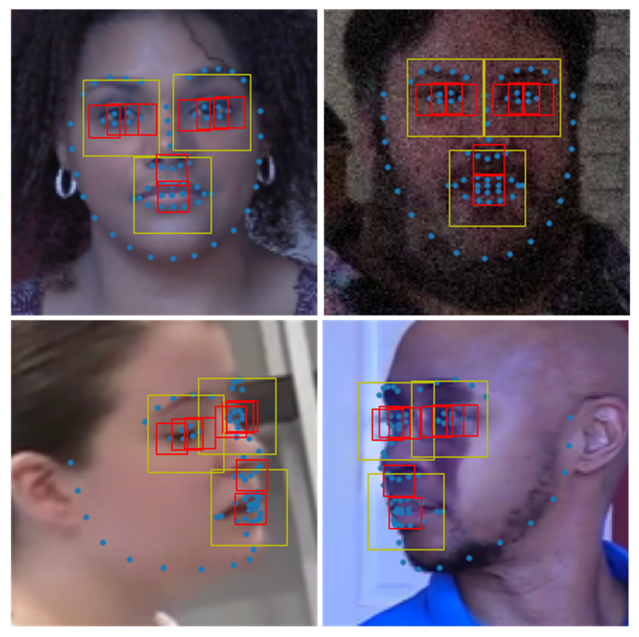
Facial landmarks are obtained by OpenFace2. With 68 facial landmarks, we crop faces with 30% of margin and resize them to $128\times 128$ with zero padding (if needed). We do not align the face since face alignment may distort the original face image and the side face is difficult to align. We conduct experiments on the discriminant power of each landmark and find that two eyes and the mouth are most discriminant regions. Thus, we crop out 8 smaller blocks that cover 6 representative landmarks from two eyes, one from the nose and one from the mouth. Furthermore, we crop out three larger blocks to cover the left eye, right eye and mouth. We make the block size a hyper-parameter for user to choose. For the experiments reported in Sec. 4, we adopt smaller blocks of size $13\times 13$ centered at landmarks and larger blocks of size $31\times 31$ for three facial regions (i.e., two eyes and the mouth) since they give the best results. The extracted small and large blocks are illustrated in Fig. 3.

3.2 Module 1: One-Stage PixelHop

A PixelHop unit (chen2019pixelhop; chen2020pixelhop++) contains a set of filters used to extract features from training blocks. While the filter weights of traditional filter banks (e.g., the Gabor or Laws filters) are fixed, those of the PixelHop are data dependent. Its filter banks are defined by the Saab transform, which decomposes a local neighborhood (i.e., a patch) into one DC (direct current) and multiple AC (alternated current) components. The DC component is the mean of each patch. The AC components are obtained through the principal component analysis (PCA) of patch residuals.

To give an example, we set the patch size to $3\times 3$ in the experiment. For the color face image input, each patch contains $(3\times 3)\times 3$ degrees of freedom, including nine spatial pixel locations and three spectral components. By collecting a large number of patches, we can conduct PCA to obtain AC filters. The eigenvectos and the eigenvalues of the covariance matrix correspond to AC filters and their mean energy values, respectively. Since most natural images are smooth, the leading AC filters extract low-frequency features of higher energy. When the frequency index goes higher, the energy of higher frequency components bdecays quickly. The Saab filter bank decouples the 27 correlated input dimensions into 27 decorrelated output dimensions. Besides decorrelating input components, the Saab transform allows to discard some high frequency channels due to their very small variances (or energy values).

The horizontal output size of a block can be calculated as

\frac{\mbox{horizontal block size}-\mbox{horizontal filter size}}{s}+1,

(1)

where $s$ is the stride parameter along the horizontal direction. For example, if the horizontal block size is 13, the horizontal filter size is 3 and the horizontal stride is 2, then the horizontal output size is equal to 6. The same computation applies to the vertical output size.

3.3 Module 2: Spatial PCA

The output of the same frequency component may still have correlations in the spatial domain. This is especially true for the DC component and low AC components. The correlation can be removed by spatial PCA. The idea of spatial PCA is inspired by the eigenface method in (turk1991eigenfaces). For each channel, we train a spatial PCA and keep the leading components that have cumulative energy up to 80% of the total energy. This helps reduce the output feature dimension.

Modules 1 and 2 describe the feature generation procedure for DefakeHop++. It is worthwhile to point out the differences in feature generation of DefakeHop and DefakeHop++.

•

DefakeHop only focuses on two eyes and mouth three regions. Besides these three regions, DefakeHop++ zooms into the neighborhood of 8 landmarks called a block to gain more detailed information. The justification of these 8 landmarks is given in the last paragraph of Sec. 4.1
•

DefakeHop conducts three-stage PixelHop units and applies spatial PCA to the response output of all three stages. The pipeline is simplfied to a one-stage PixelHop in DefakeHop++. Yet, the simplification does not hurt the performance since the spatial PCA applied to each block (or region) still offer the global information of the corresponding block (or region). Note that such simplification is needed as DefakeHop++ covers more spatial patches and regions.

3.4 Module 3: Discriminant Feature Test

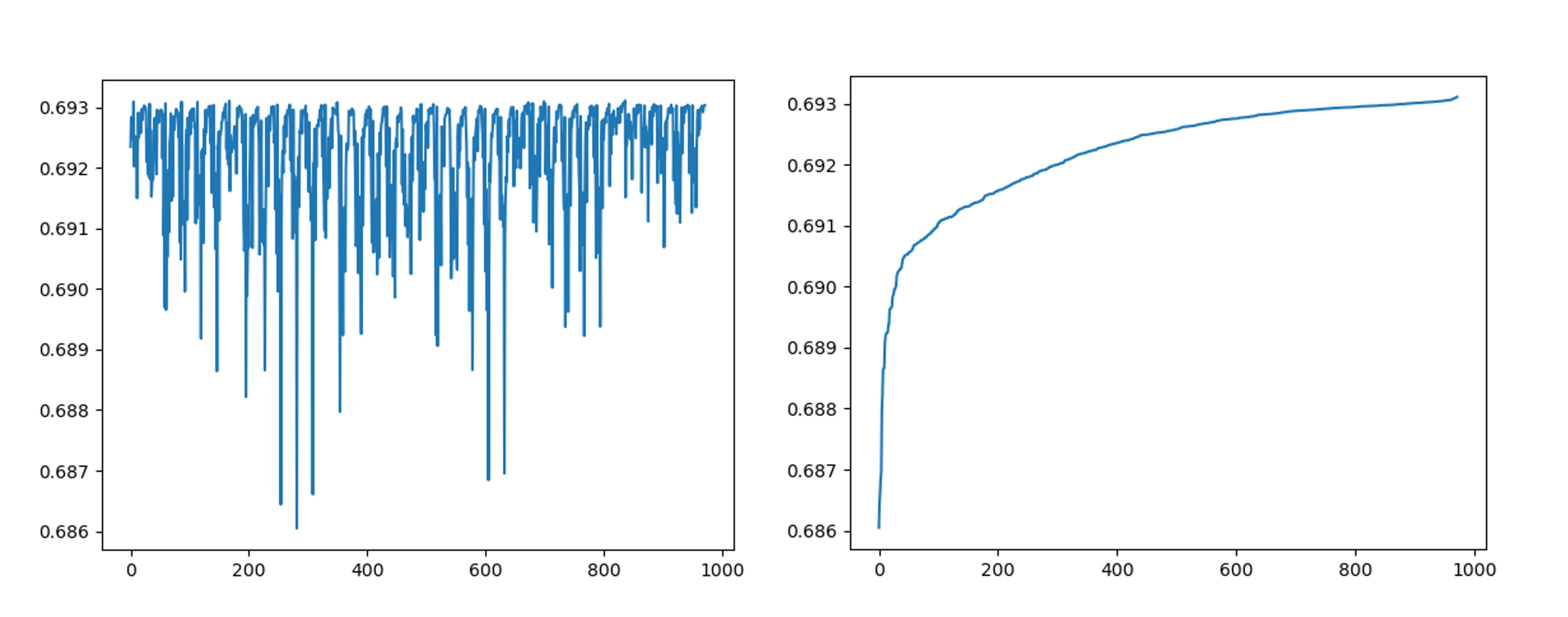
DefakeHop selects responses from channels of larger energy as features into a classifier under the assumption that features of higher variance are more discriminant. This is an unsupervised feature selection method. Recently, a supervised feature selection method called the discriminant feature test (DFT) was proposed in (yang2022supervised). DFT provides a powerful method in selecting discriminant features using training labels. The DFT process can be simply stated below. For each feature dimension, we define an interval using its minimum and maximum values across all training samples. Then, we partition the interval into two sub-intervals at all possible split positions which are equally spaced in the interval. For example, if we may select 31 split positions uniformly distributed over the interval. For each partitioning, we can use the maximum likelihood principle to assign a predicted label to each training sample and compute the cross entropy of all training samples accordingly. The split position that gives the lowest cross entropy is chosen to be the optimal split of the feature and the associated cross entropy is used as the cost function of this feature. The lower the cross entropy, the most discriminant the feature dimension. We refer to (yang2022supervised) for more details.

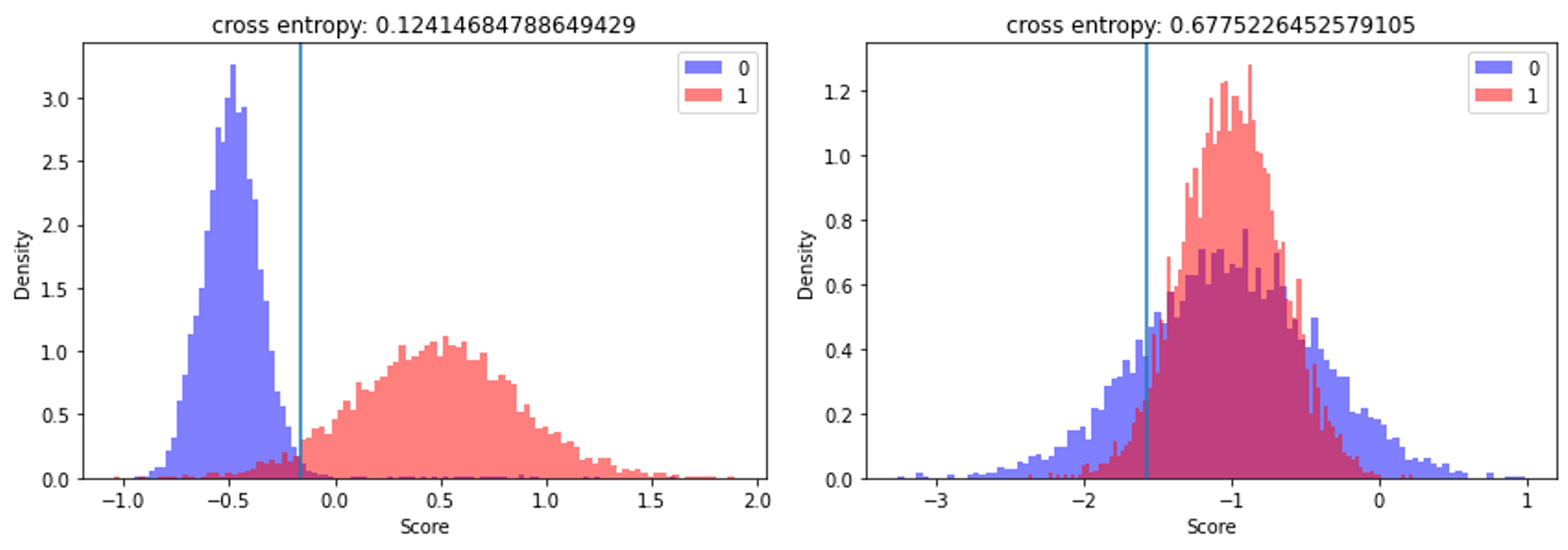
We use Figs. 4 and 5 to explain the DFT idea. Two features are compared in Fig. 4. The feature in the left subfigure has a lower cross entropy value than the one in the right subfigure. The left one is more discriminant than the right one, which is intuitive. Fig. 5 is used to describe the feature selection process for a given landmark block. The feature dimension of one landmark block is 972. We perform DFT on each feature and obtain 972 cross entropy values. The y-axis in both subfigures is the cross entropy value while the x-axis is the channel index. In the left subfigure, a smaller channel index indicates a lower frequency channel. We see that discriminant channels of lower cross entropy actually spread out in both low and high frequency channels. In the right plot, we sort channels based on their cross entropy values, which have an elbow point at 350. As a result, we can reduce the feature number from 972 to 350 (35%) by selecting 350 features with the lowest cross entropy.

3.5 Module 4: Classification

In DefakeHop, soft decisions from different regions are used to train several XGBoost classifiers. Then, another ensemble XGBoost classifier is trained to make the final decision. This is a two-stage decision process. We find that a lot of detailed information is lost in the first-stage soft decisions and, as a result, the ensemble classification idea is not effective. To address this issue, we simply collect all feature vectors from different regions and landmarks, apply DFT for discriminant feature selection and train a LightGBM classifier in the last stage in DefakeHop++. LightGBM and XGBoost play a similar role. The main difference between DefakeHop and DefakeHop++ is that the former is a two-stage decision process while the latter is a one-stage decision process. The one-stage decision process can consider the complicated relations of features in landmarks and regions across all frequency bands. Once all frame-level predictions for a video are obtained, we simply use their mean as the final prediction for the video.

Table 1: Comparison of detection performance of several methods on the first genreation datasets with AUC as the performance metric. The AUC results of DefakeHop++ in both frame-level and video-level are given. The best and the second-best results are shown in boldface and underbared, respectively. The AUC results of benchmarking methods are taken from li2020celeb and the number of parameters are from https://keras.io/api/applications. Also, we use ^a to denote deep learning methods and ^b to denote non-deep-learning methods.

		1st Generation
Method	Model	UADFV	FF++	#param
Two-stream (zhou2017two)	InceptionV3^a(szegedy2016rethinking)	85.1%	70.1%	23.9M
Meso4 (afchar2018mesonet)	Designed CNN^a	84.3%	84.7%	28.0K
MesoInception4 (afchar2018mesonet)	Designed CNN^a	82.1%	83.0%	28.6K
HeadPose (yang2019exposing)	SVM^b	89.0%	47.3%	-
FWA (li2018exposing)	ResNet-50^a(he2016deep)	97.4%	80.1%	25.6M
VA-MLP (matern2019exploiting)	Designed CNN^a	70.2%	66.4%	-
VA-LogReg (matern2019exploiting)	Logistic Regression^b	54.0%	78.0%	-
Xception-raw (rossler2019faceforensics++)	XceptionNet^a(chollet2017xception)	80.4%	99.7%	22.9M
Xception-c23 (rossler2019faceforensics++)	XceptionNet^a(chollet2017xception)	91.2%	99.7%	22.9M
Xception-c40 (rossler2019faceforensics++)	XceptionNet^a(chollet2017xception)	83.6%	95.5%	22.9M
Multi-task (nguyen2019multi)	Designed CNN^a	65.8%	76.3%	-
Capsule (nguyen2019use)	CapsuleNet^a(sabour2017dynamic)	61.3%	96.6%	3.9M
DSP-FWA (li2019exposing)	SPPNet^a(he2015spatial)	97.7%	93.0%	-
Multi-attentional (zhao2021multi)	Efficient-B4^a(tan2019efficientnet)	-	99.8%	19.5M
DefakeHop (chen2021defakehop)	DefakeHop^b	100%	96.0%	42.8K
Ours (Frame Level)	DefakeHop++^b	100%	98.4%	238K
Ours (Video Level)	DefakeHop++^b	100%	99.3%	238K

Table 2: Comparison of detection performance of several Deepfake detectors on the second genreation datasets under cross-domain training and with AUC as the performance metric. The AUC results of DefakeHop anad DefakeHop++ in both frame-level and video-level are given. The best and the second-best results are shown in boldface and underbared, respectively. Furthermore, we include results of DefakeHop and DefakeHop++ under the same-domain training in the last 4 rows. The AUC results of benchmarking methods are taken from li2020celeb and the number of parameters are from https://keras.io/api/applications. Also, we use ^a to denote deep learning methods and ^b to denote non-deep-learning methods.

		2nd Generation
Method	Model	Celeb-DF v1	Celeb-DF v2	#param
Two-stream (zhou2017two)	InceptionV3^a	55.7%	53.8%	23.9M
Meso4 (afchar2018mesonet)	Designed CNN^a	53.6%	54.8%	28.0K
MesoInception4 (afchar2018mesonet)	Designed CNN^a	49.6%	53.6%	28.6K
HeadPose (yang2019exposing)	SVM^b	54.8%	54.6%	-
FWA (li2018exposing)	ResNet-50^a	53.8%	56.9%	25.6M
VA-MLP (matern2019exploiting)	Designed CNN^a	48.8%	55.0%	-
VA-LogReg (matern2019exploiting)	Logistic Regression^b	46.9%	55.1%	-
Xception-raw (rossler2019faceforensics++)	XceptionNet^a	38.7%	48.2%	22.9M
Xception-c23 (rossler2019faceforensics++)	XceptionNet^a	-	65.3%	22.9M
Xception-c40 (rossler2019faceforensics++)	XceptionNet^a	-	65.5%	22.9M
Multi-task (nguyen2019multi)	Designed CNN^a	36.5%	54.3%	-
Capsule (nguyen2019use)	CapsuleNet^a	-	57.5%	3.9M
DSP-FWA (li2019exposing)	SPPNet^a	-	64.6%	-
Multi-attentional (zhao2021multi)	Efficient-B4^a	-	67.4%	19.5M
Ours (Frame Level)	DefakeHop++^b	56.30%	60.5%	238K
Ours (Video Level)	DefakeHop++^b	58.15%	62.4%	238K
Ours (Trained on Celeb-DF, Frame Level)	DefakeHop^b	93.1%	87.7%	42.8K
Ours (Trained on Celeb-DF, Video Level)	DefakeHop^b	95.0%	90.6%	42.8K
Ours (Trained on Celeb-DF, Frame Level)	DefakeHop++^b	95.4%	94.3%	238K
Ours (Trained on Celeb-DF, Video Level)	DefakeHop++^b	97.5%	96.7%	238K

4 Experiments

We compare the detection performance of DefakeHop++, state-of-the-art deep learning and non-deep learning methods on several datasets as well as their model sizes and training time in this section to demonstrate the effectiveness of DefakeHop++.

4.1 Experimental Setup

Datasets. Deepfake video datasets can be categorized into three generations based on the dataset size and Deepfake methods used for fake image generation. The first-generation datasets includes UADFV and FF++. The second-generation datasets include Celeb-DF version 1 and version 2. The third-generation dataset is the DFDC dataset. The datasets of later generations have more identities of different races, utilize more deepfake algorithms to generate fake videos, and add more perturbation types to test videos. Apparently, the later generation is more challenging than the earlier generation. The datasets used in our experiments are described below.

•

UADFV (li2018exposing)
UADFV is the first Deepfake detection dataset. It consists of 49 real videos and 49 fake videos. Real videos are collected from YouTube while fake ones are generated by the FakeApp mobile App (Fakeapp).
•

FaceForensics++ (FF++) (rossler2019faceforensics++)
It contains 1000 real videos collected from YouTube. Two popular methods, FaceSwap (Kowalski2016) and Deepfakes (Deepfakes2018), are used in fake video generation. Each of them generated 1000 fake videos of different quality levels, e.g., RAW, HQ (high quality) and LQ (low quality). In the experiment, we focus on HQ compressed videos since they are more challenging to detect by Deepfake detection algorithms.
•

Celeb-DF (li2020celeb)
Celeb-DF has two versions. Celeb-DF v1 contains 408 real videos from YouTube and 795 fake videos. Celeb-DF v2 consists of 890 real and 5639 fake videos. Fake videos are created by an advanced version of DeepFake. These videos contain subjects of different ages, ethnicities and sex. Celeb-DF v2 is a superset of Celeb-DF v1. Celeb-DF v1 and v2 have been widely tested on many Deepfake detection methods.
•

DFDC (dolhansky2020deepfake)
DFDC is the third generation dataset. It contains more than 100K videos generated by 8 different Deepfake algorithms. The test videos are perturbed by 19 distractors and augmenters such as change of brightness/contrast, logo overlay, dog filter, dots overlay, faces overlay, flower crown filter, grayscale, horizontal flip, noise, images overlay, shapes overlay, change of coding quality level, rotation, text overlay, etc. The dataset was generated to mimic the real-world application scenario. It is the most challenging one among the four benchmark datasets.

Evaluation Metrics. Each Deepfake detector assigns a probability score of being a fake one to all test images. Then, these scores can be used to plot the Receiver Operating Characteristic (ROC) curve. Then, the area under curve (AUC) score can be used to compare the performance of different detectors. We report the AUC scores at the frame level as well as the video level.

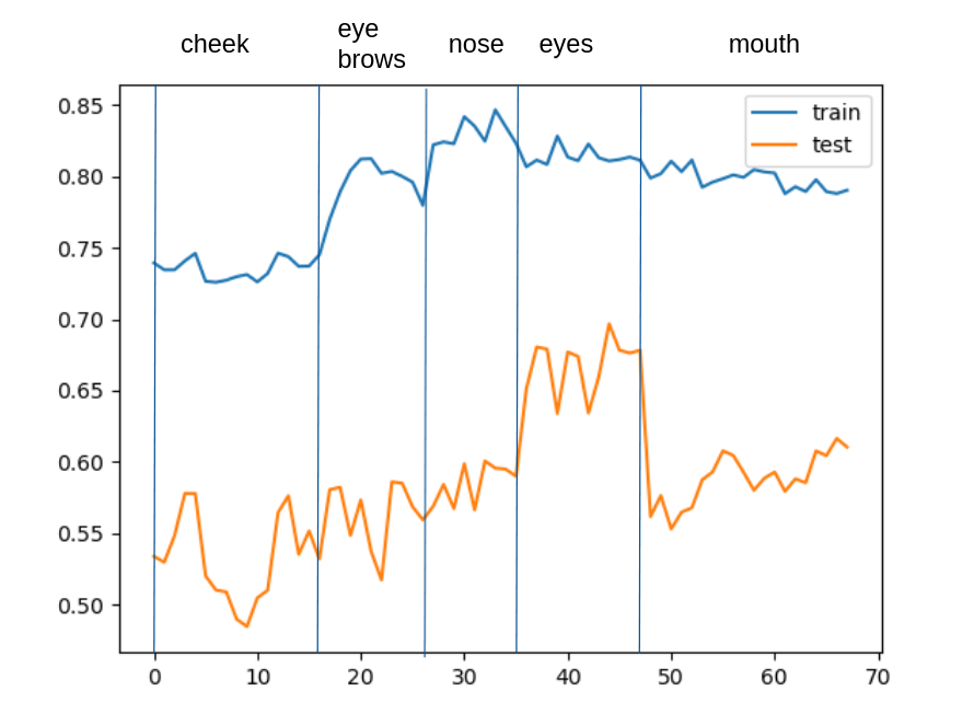
Discriminability Analysis of Landmarks. As mentioned in Sec. 3.1, there are 68 landmarks. We use the AUC scores to analyze the discriminability of the 68 landmark regions in Fig. 6. We see from the figure that the performance of different landmarks varies a lot. Landmarks in two eye regions are most discriminant. This is attributed to the fact that eyes have rich details and complex movement and, as a result, they cannot be well synthesized by any Deepfake algorithms. The mouth region is the next discriminant one because it is difficult to synthesize lip motion and teeth. The cheek and nose regions are less discriminant since they are relatively smooth in space and stable in time. This justifies our choice of six landmarks from eyes, one landmark from the nose and one landmark from the mouth as described in Sec. 3.1.

4.2 Detection Performance Comparison

First Generation Datasets. The performance of a few Deepfake detectors on two first generation datasets, UADFV and FF++, is compared in Table 1. Both DefakeHop and DefakeHop++ achieve a perfect AUC score of 100% against UADFV. DSP-FWA and FWA are two closer ones with AUC scores of 97.7% and 97.4%, respectively. Actually, UADFV is an easy dataset where the visual artifacts are visible to human eyes. It is interesting to see that the extremely large models do not reach perfect detection results. This could be explained by the small size of UADFV (i.e., 49 real videos and 49 fake videos). The model sizes of DefakeHop and DefakeHop++ can be sufficiently trained by a small dataset size. For FF++, Multi-attentional achieves the best AUC score (i.e., 99.8%) while Xception-raw and Xception-c23 achieves the second best (i.e., 99.7%). DefakeHop++ with its AUC computation at the videl level has the next highest AUC score (i.e., 99.3%). The performance gap among them is small. Furthermore, the performance of Xception-raw and Xception-c23 is boosted by a larger dataset size of FF++, which has 1000 real videos of different quality levels.

Second Generation Datasets with Cross-Domain Training. The performance of several Deepfake detectors, which are trained on the FF++ dataset, against two second generation datasets is compared in Table 2. We see that video-level DefakeHop++ gives the best AUC score while frame-level DefakeHop++ gives the second best AUC score for Celeb-DF-v1. As to Celeb-DF-v2, Multi-attentional yield the best AUC score while Xception-raw and Xception-c23 offer the second best scores. DefakeHop++ is slightly inferior to them. Furthermore, we show the performance of DefakeHop and DefakeHop++ under the same domain training in the last four rows of Table 2. Their performance has improved significantly. Video-level DefakeHop++ outperforms video-level DefakeHop by 2.5% in Celeb-DF v1 and 6.1% in Celeb-DF v2.

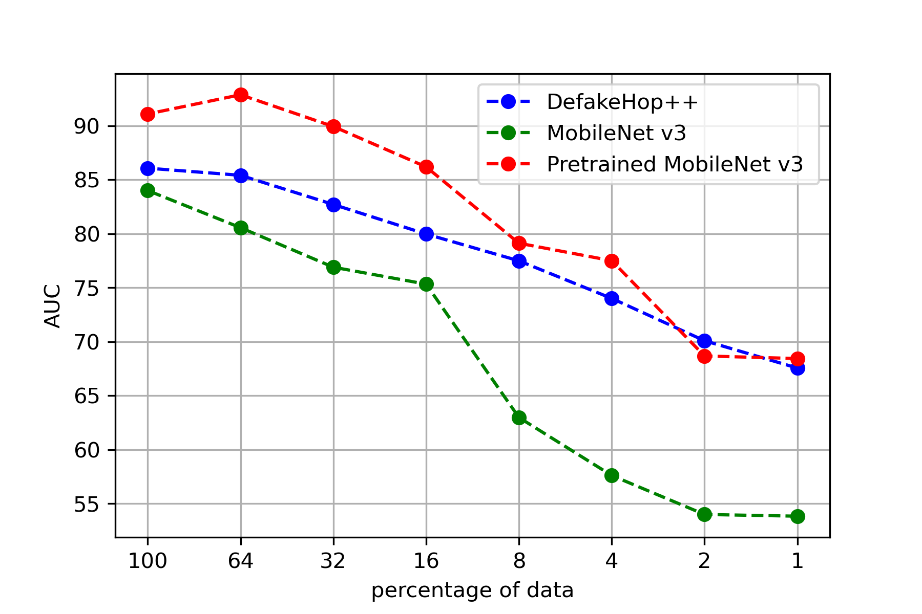
Third Generation Dataset. The size of the third generation dataset, DFDC, is huge. It demands a lot of computational resources (including training hardware, time and large models) to achieve high performance. Since our main interest is on lightweight detection algorithms, we focus on the comparison of DefakeHop++ and MobileNet v3, which has 1.5M parameters and targets at mobile applications. We train both models with parts and/or all of DFDC training data and report the detection performance on the test dataset in Fig. 7. We have the following three observations from the figure. First, pre-trained MobileNet v3 gives the best result, DefakeHop++ the second, and MobileNet v3 without pre-training the worst. It shows that, if there are sufficient training data in training, the detection performance of a larger model can be boosted. For the same reason, the detection performance of all three models decreases as the training data of DFDC becomes less. Second, with 1-8% of DFDC training data, the performance of DefakeHop++ and pre-trained MobileNet v3 is actually very close. The performance gap between DefakeHop++ and MobileNet v3 without pre-training is significant in all training data ranges. For example, with only 1% of the DFDC training data, the AUC score of DefakeHop++ reaches 68% while that of MobileNet V3 can only reach 54%. Third, with 100% of the DFDC training data but without any data augmentation, DefakeHop++ still can achieve an AUC score of 86%, which is 5% lower than pre-trained MobileNet v3.

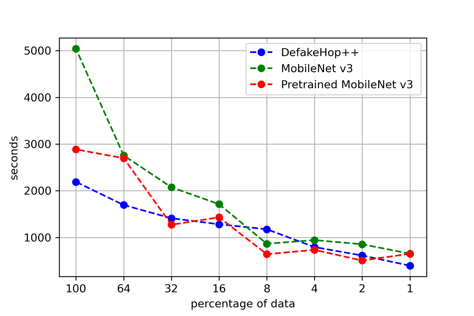
Furthermore, we compare the training time on the three models as a function of the training data percentage in Fig. 8. The model is trained on AMD Ryzen 9 5950X with Nvidia GPU 3090 24G. If a CNN is not pre-trained, it generally needs more time to converge. The training time of DefakeHop++ is lowest for 64% and 100% of the total training data. Its training time is about the same as the pre-trained MobileNet v3 for the cases of 1-32% training data.

4.3 Model Size of DefakeHop++

DefakeHop++ consists of one-stage PixelHop, Spatial PCA, DFT and Classifier modules. The size of each component can be computed as follows.

PixelHop. The parameters are the filter weights. Each filter has a size of $(3\times 3)\times 3=27$ . Since there are 27 filters, the total number of parameters of PixelHop is $27\times 27=729$ parmaeters.

Spatial PCA. For each channel, we flatten 2D spatial responses to a 1D vector and train a PCA. We conduct spatial PCA on channels of higher energy (i.e. those with cumulative energy up to 80% total energy). Furthermore, we set an upper limit of 10 channels to avoid a large number of filters for a particular channel. Based on this design guideline, the averaged channel numbers for a landmark and a spatial region are 35 and 40, respectively.

DFT. DFT is used to select a subset of discriminant features. Its parameters are indices of selected channels. For 8 landmark blocks, we keep features in top 35%. For 3 spatial regions, we keep features in top 15%. Then, the number of parameters of DFT is $(8\times 340)+(3\times 911)=5,453$ as shown in Table 3.

Classifier. We use LightGBM (ke2017lightgbm) as the classifier and set the maximum number of leaves to 64. As a result, the maximum intermediate node number of a tree is bounded by 63. We store two parameters (i.e., the selected dimension and its threshold) at each intermediate node and one parameter (i.e., the predicted soft decision score) at each leaf node. The number of parameters for one tree is bounded by 190. Furthermore, we set the maximum number of tree to 1000. Thus, the number of parameters for LightGBM is bounded by 190K.

Table 3: The number of parameters for various parts.

	Subsystem	Number	Parameters	Total
Pixelhop	Landmarks	8	3x3x3=729	5832
Pixelhop	Regions	3	3x3x3=729	2187
Spatial PCA	Landmarks	8	6x6x35=1,260	10,080
Spatial PCA	Regions	3	15x15x40=9,000	27,000
DFT	Landmarks	8	6x6x27x0.35=340	2720
DFT	Regions	3	15x15x27x0.15=911	2733
LightGBM	-	1	190,000	190,000
Total				237,832

5 Conclusion and Future Work

A lightweight Deepfake detection method, called DefakeHop++, was proposed in this work. It is an enhanced version of our previous solution called DefakeHop. Its model size is significantly smaller than that of state-of-the-art DNN-based solutions, including MobileNet v3, while keeping reasonably high detection performance. It is most suitable for Deepfake detection in mobile/edge devices.

Fake image/video detection is an important topic. The faked content is not restricted to talking head videos. There are many other application scenarios. Examples include faked satellite images, image splicing, image forgery in publications, etc. Heavyweight fake image detection solutions are not practical. Furthermore, fakes images can appear in many forms. On one hand, it is unrealistic to include all possible perturbations in the training dataset under the setting of heavy supervision. On the other hand, the performance could be quite poor with little supervision. It is essential to find a midground and look for a lightweight weakly-supervised solution with reasonable performance. This paper shows our research effort along this direction. We will continue to explore and generalize the mothodology to other challenging Deepfake problems.

\printbibliography