A universal robust limit theorem for nonlinear Lévy processes under sublinear expectation

Abstract. This article establishes a universal robust limit theorem under a sublinear expectation framework. Under moment and consistency conditions, we show that, for $\alpha\in(1,2)$, the i.i.d. sequence

$$\left\{\left(\frac{1}{\sqrt{n}}\sum_{i=1}^{n}X_{i},\frac{1}{n}\sum_{i=1}^{n}Y_{i},\frac{1}{\sqrt[\alpha]{n}}\sum_{i=1}^{n}Z_{i}\right)\right\}_{n=1}^{\infty}$$

converges in distribution to $\tilde{L}_{1}$, where $\tilde{L}_{t}=(\tilde{\xi}_{t},\tilde{\eta}_{t},\tilde{\zeta}_{t})$, $t\in[0,1]$, is a multidimensional nonlinear Lévy process with an uncertainty set $\Theta$ as a set of Lévy triplets. This nonlinear Lévy process is characterized by a fully nonlinear and possibly degenerate partial integro-differential equation (PIDE)

$$\left\{\begin{array}[c]{l}\displaystyle\partial_{t}u(t,x,y,z)-\sup\limits_{(F_{\mu},q,Q)\in\Theta}\left\{\int_{\mathbb{R}^{d}}\delta_{\lambda}u(t,x,y,z)F_{\mu}(d\lambda)\right.\\ \displaystyle\text{\ \ \ \ \ \ \ \ \ \ \ \ \ \ \ \ }\left.+\langle D_{y}u(t,x,y,z),q\rangle+\frac{1}{2}tr[D_{x}^{2}u(t,x,y,z)Q]\right\}=0,\\ \displaystyle u(0,x,y,z)=\phi(x,y,z),\ \ \forall(t,x,y,z)\in[0,1]\times\mathbb{R}^{3d},\end{array}\right.$$

with $\delta_{\lambda}u(t,x,y,z):=u(t,x,y,z+\lambda)-u(t,x,y,z)-\langle D_{z}u(t,x,y,z),\lambda\rangle$. To construct the limit process $(\tilde{L}_{t})_{t\in[0,1]}$, we develop a novel weak convergence approach based on the notions of tightness and weak compactness on a sublinear expectation space. We further prove a new type of Lévy-Khintchine representation formula to characterize $(\tilde{L}_{t})_{t\in[0,1]}$. As a byproduct, we also provide a probabilistic approach to prove the existence of the above fully nonlinear degenerate PIDE.

Key words. Universal robust limit theorem, Partial integro-differential equation, Nonlinear Lévy process, $\alpha$-stable distribution, Sublinear expectation

MSC-classification. 60F05, 60G51, 60G52, 60G65, 45K05

1 Introduction

Motivated by measuring risks under model uncertainty, Peng [25, 26, 27, 31] introduced the notion of sublinear expectation space, called $G$-expectation space. The $G$-expectation theory has been widely used to evaluate random outcomes, not using a single probability measure, but using the supremum over a family of possibly mutually singular probability measures.

One of the fundamental results in the theory is Peng’s robust central limit theorem introduced in [28, 30, 31]. Let $\{(X_{i},Y_{i})\}_{i=1}^{\infty}$ be an i.i.d. sequence of random variables on a sublinear expectation space $(\Omega,\mathcal{H},\mathbb{\hat{E}})$. Under certain moment conditions, Peng proved that there exists a $G$-distributed random variable $(\xi,\eta)$ such that

$$\lim_{n\rightarrow\infty}\mathbb{\hat{E}}\bigg{[}\phi\bigg{(}\frac{1}{\sqrt{n}}\sum_{i=1}^{n}{X_{i}},\frac{1}{n}\sum_{i=1}^{n}Y_{i}\bigg{)}\bigg{]}=\mathbb{\tilde{E}}[\phi(\xi,\eta)],$$

for any test function $\phi$. The $G$-distributed random variables $(\xi,\eta)$ describes volatility and mean uncertainty, and can be characterized via a fully nonlinear parabolic PDE, i.e., the function $u(t,x,y):=\mathbb{\tilde{E}}[\phi(x+\sqrt{t}\xi,y+t\eta)]$ solves

$$\left\{\begin{array}[c]{l}\partial_{t}u(t,x,y)-G(D_{y}u,D_{x}^{2}u)=0,\\ u(0,x,y)=\phi(x,y),\end{array}\right.$$ (1.1)

where the sublinear function

$$G\left(p,A\right):=\mathbb{\hat{E}}\left[\frac{1}{2}\left\langle AX_{1},X_{1}\right\rangle+\left\langle p,Y_{1}\right\rangle\right],\ (p,A)\in\mathbb{R}^{d}\times\mathbb{S(}d\mathbb{)}.$$

This limit theorem was established by Peng around 2008 (see [28]) using the regularity theory of fully nonlinear PDEs from [6, 18, 36]. The corresponding convergence rate was established by Fang et al [11] and Song [35] using Stein’s method and later by Krylov [19] using stochastic control method under different model assumptions. More recently, Huang and Liang [16] studied the convergence rate of a more general central limit theorem via a monotone approximation scheme.

To further describe jump uncertainty, Hu and Peng [14, 15] introduced a class of nonlinear Lévy processes with finite activity jumps, called $G$-Lévy processes in the setting of sublinear expectation, and built a type of Lévy-Khintchine representation for $G$-Lévy processes by relating to a class of fully nonlinear partial integro-differential equations (PIDEs). For given characteristics, more general nonlinear Lévy processes with infinite activity jumps have been studied by Neufeld and Nutz [24] (see also [8, 20, 23]). An important class of nonlinear Lévy processes is the $\alpha$-stable process $(\zeta_{t})_{t\geq 0}$ for $\alpha\in(1,2)$, whose characteristic is described by an uncertainty set $\Theta_{0}=\{(F_{k_{\pm}},0,0):k_{\pm}\in K_{\pm}\}$, where $K_{\pm}\subset(\lambda_{1},\lambda_{2})$ for some $\lambda_{1},\lambda_{2}>0$, $(0,0)$ means that $(\zeta_{t})_{t\geq 0}$ is a pure jump Lévy process without diffusion and drift, and $F_{k_{\pm}}(dz)$ is the $\alpha$-stable Lévy measure

$$F_{k_{\pm}}(dz)=\frac{k_{-}}{|z|^{\alpha+1}}\mathbf{1}_{(-\infty,0)}(z)dz+\frac{k_{+}}{|z|^{\alpha+1}}\mathbf{1}_{(0,\infty)}(z)dz.$$

The nonlinear $\alpha$-stable process $(\zeta_{t})_{t\geq 0}$ on a sublinear expectation space $(\Omega,\mathcal{H},\mathbb{\tilde{E}})$ can be characterized via a fully nonlinear PIDE, i.e., the function $u(t,x):=\mathbb{\tilde{E}}[\phi(x+\zeta_{t})]$ solves

$$\left\{\begin{array}[c]{l}\displaystyle\partial_{t}u(t,x)-\sup\limits_{k_{\pm}\in K_{\pm}}\left\{\int_{\mathbb{R}}\delta_{\lambda}u(t,x)F_{k_{\pm}}(d\lambda)\right\}=0,\\ \displaystyle u(0,x)=\phi(x),\end{array}\right.$$ (1.2)

where $\delta_{\lambda}u(t,x):=u(t,x+\lambda)-u(t,x)-D_{x}u(t,x)\lambda$.

The corresponding limit theorem for $\alpha$-stable processes under sublinear expectation was established by Bayraktar and Munk [5]. Let $\{Z_{i}\}_{i=1}^{\infty}$ be an i.i.d. sequence of real-valued random variables on a sublinear expectation space $(\Omega,\mathcal{H},\mathbb{\hat{E})}$ satisfying certain moment and consistency conditions, they proved that there exists a nonlinear $\alpha$-stable process $(\zeta_{t})_{t\geq 0}$ such that

$$\lim_{n\rightarrow\infty}\mathbb{\hat{E}}\bigg{[}\phi\bigg{(}\frac{1}{\sqrt[\alpha]{n}}\sum_{i=1}^{n}Z_{i}\bigg{)}\bigg{]}=\mathbb{\tilde{E}}[\phi(\zeta_{1})],$$

for any test function $\phi$. Their proof relies on the interior regularity results of fully nonlinear PIDEs from [6, 21, 22]. More recently, Hu et al [13] established the corresponding convergence rate via a monotone approximation scheme.

The aim of this article is to study the robust limit theorem for a multidimensional nonlinear Lévy process under a sublinear expectation framework. To be more specific, let $\{(X_{i},Y_{i},Z_{i})\}_{i=1}^{\infty}$ be an i.i.d. sequence of $\mathbb{R}^{3d}$-valued random variables on a sublinear expectation space $(\Omega,\mathcal{H},\mathbb{\hat{E})}$ and $\alpha\in(1,2)$. Then, the first question is under what conditions does the following i.i.d. sequence

$$\left\{\left(\frac{1}{\sqrt{n}}\sum_{i=1}^{n}X_{i},\frac{1}{n}\sum_{i=1}^{n}Y_{i},\frac{1}{\sqrt[\alpha]{n}}\sum_{i=1}^{n}Z_{i}\right)\right\}_{n=1}^{\infty}$$

converge? If so, then the second question is how to characterize the limit? We provide affirmative answers for both questions in Theorem 3.4, which is dubbed as a universal robust limit theorem under sublinear expectation. The result covers all the existing robust limit theorems in the literature, namely, Peng’s robust central limit theorem for $G$-distribution (see [28]) and Bayraktar-Munk’s robust limit theorem for $\alpha$-stable distribution (see [5]). One remarkable feature of the result is that $(X_{1},Y_{1},Z_{1})$ may depend on each other, so one cannot simply combine the robust limit theorems in [5] and [28]. Moreover, the conditions that we propose are mild. In fact, they are weaker than the characterization condition proposed in linear setting (see Remark 3.3) and the consistency condition in nonlinear setting (see Remark 3.2).

On the other hand, the existing methods for the robust limit theorems do not work, because [5, 28] reply on the regularity estimates of the fully nonlinear PDE (1.1) and PIDE (1.2). However, the required regularity for the general equation (3.3) in Theorem 3.4 is unknown to date. Moreover, it seems that most of the existing methods are analytical and heavily rely on the regularity theory. It is natural to ask whether one can establish a probabilistic proof as in the classical linear expectation case. As expected, weak convergence plays a pivotal role. Peng [29] firstly introduced the notions of tightness and weak compactness on a sublinear expectation space and provided an alternative proof for his robust central limit theorem. In Theorem 4.1, we further develop this weak convergence approach to establish a Donsker-type result showing that the limit indeed exists and is a nonlinear Lévy process $\tilde{L}_{t}:=(\tilde{\xi}_{t},\tilde{\eta}_{t},\tilde{\zeta}_{t})$ at $t=1$ with $(\tilde{\xi}_{1},\tilde{\eta}_{1})$ following $G$-distribution.

A more challenging task is to characterize the third component $\tilde{\zeta}_{t}$ and also $\tilde{L}_{t}$ as a whole. This will in turn link the nonlinear Lévy process $(\tilde{L}_{t})_{t\in[0,1]}$ with the fully nonlinear PIDE (3.3). However, the proofs for the classical linear expectation cases (e.g. CLT and $\alpha$-stable limit theorem) are to a considerable extent based on characteristic function techniques, which do not exist in the sublinear framework. A new type of Lévy-Khintichine formula is therefore needed. Note that the proof of this representation formula is also an important open question left in the literature (see Remark 23 in [15] and Page 71 in [24]). We overcome this difficulty by deriving a new estimate for the $\alpha$-stable Lévy measure (see Theorem 4.5), which in turn enables us to prove a new type of Lévy-Khintichine representation formula for the nonlinear Lévy process (see Theorem 4.7). Thanks to the connection with the fully nonlinear PIDE (3.3), we also obtain the existence of its viscosity solution as a byproduct.

The article is organized as follows. In Section 2, we review some necessary results about sublinear expectation. Section 3 details our main result: the universal robust limit theorem in Theorem 3.4. The proofs of the main theorem is given in Section 4. Finally, an example highlighting the applications of our main result is given in Section 5.

2 Preliminaries

This section briefly introduces notions and preliminaries in the sublinear expectation framework. For more details, we refer the reader to [26, 27, 29, 31] and the references therein.

2.1 Sublinear expectation

Let $\Omega$ be a given set and let $\mathcal{H}$ be a linear space of real valued functions defined on $\Omega$ such that $1\in\mathcal{H}$ and $|X|\in\mathcal{H}$ if $X\in\mathcal{H}$. Then, a sublinear expectation is defined as follows.

Definition 2.1

A functional $\mathbb{\hat{E}}$: $\mathcal{H}\rightarrow\mathbb{R}$ is called a sublinear expectation if, for all $X,Y\in\mathcal{H}$, it satisfies the following properties.

(i)

(Monotonicity) $\mathbb{\hat{E}}[X]\geq\mathbb{\hat{E}}[Y]$, if $X\geq Y$;

(ii)

(Constant preservation) $\mathbb{\hat{E}}[c]=c$, for $c\in\mathbb{R}$;

(iii)

(Sub-additivity) $\mathbb{\hat{E}}[X+Y]\leq\mathbb{\hat{E}}[X]+\mathbb{\hat{E}}[Y];$

(iv)

(Positive homogeneity) $\mathbb{\hat{E}}[\lambda X]=\lambda\mathbb{\hat{E}}[X]$, for $\lambda>0$.

The triplet $(\Omega,\mathcal{H},\mathbb{\hat{E})}$ is called a sublinear expectation space. From the definition of the sublinear expectation $\mathbb{\hat{E}}$, the following results can be easily obtained.

Proposition 2.2

For $X,Y$ $\in\mathcal{H}$, we have

(i)

if $\mathbb{\hat{E}}[X]=-\mathbb{\hat{E}}[-X]$, then $\mathbb{\hat{E}}[X+Y]=\mathbb{\hat{E}}[X]+\mathbb{\hat{E}}[Y];$

(ii)

$|\mathbb{\hat{E}}[X]-\mathbb{\hat{E}}[Y]|\leq\mathbb{\hat{E}}[|X-Y|]$, i.e., $|\mathbb{\hat{E}}[X]-\mathbb{\hat{E}}[Y]|\leq\mathbb{\hat{E}}[X-Y]\vee\mathbb{\hat{E}}[Y-X];$

(iii)

$\mathbb{\hat{E}}[|XY|]\leq(\mathbb{\hat{E}}[|X|^{p}])^{1/p}(\mathbb{\hat{E}}[|Y|^{q}])^{1/q},$ for $1\leq p,q<\infty$ with $\frac{1}{p}+\frac{1}{q}=1.$

Definition 2.3

We say $X_{1}$ on a sublinear expectation space $(\Omega_{1},\mathcal{H}_{1},\hat{E}_{1})$ and $X_{2}$ on another sublinear expectation space $(\Omega_{2},\mathcal{H}_{2},\mathbb{\hat{E}}_{2})$ identically distributed, if $\mathbb{\hat{E}}_{1}[\varphi(X_{1})]=\mathbb{\hat{E}}_{2}[\varphi(X_{2})]$, for all $\varphi\in{C_{b,Lip}}(\mathbb{R}^{n})$, the space of bounded Lipschitz continuous functions on $\mathbb{R}^{n}$.

The concept of independence plays a pivotal role in sublinear expectation. Notably, $Y$ is independent from $X$ does not necessarily imply that $X$ is independent from $Y$.

Definition 2.4

Let $(\Omega,\mathcal{H},\mathbb{\hat{E})}$ be a sublinear expectation space. An $n$-dimensional random variable $Y$ is said to be independent from another $m$-dimensional random variable $X$ under $\mathbb{\hat{E}}[\cdot]$, denoted by $Y\perp\!\!\!\perp X$, if for every test function $\varphi\in C_{b,Lip}(\mathbb{R}^{m}\times\mathbb{R}^{n})$ we have

$$\mathbb{\hat{E}}\left[\varphi(X,Y)\right]=\mathbb{\hat{E}}\left[\mathbb{\hat{E}}\left[\varphi(x,Y)\right]_{x=X}\right].$$

$\bar{X}$ is said to be an independent copy of $X$ if $\bar{X}\overset{d}{=}X$ and $\bar{X}\perp\!\!\!\perp X$.

The independence assumption implies the additivity of $\mathbb{\hat{E}}$ as shown in the following proposition.

Proposition 2.5

For $X,Y\in\mathcal{H}$, if $Y\perp\!\!\!\perp X$, then

$$\mathbb{\hat{E}}[X+Y]=\mathbb{\hat{E}}[X]+\mathbb{\hat{E}}[Y].$$

2.2 Tightness, weak compactness, and convergence in distribution

Weak convergence plays an important role in establishing the universal robust limit theorem. The following definitions of tightness and weak compactness are adapted from Peng [29, Definitions 7 and 8].

Definition 2.6

A sublinear expectation $\mathbb{\hat{E}}$ on $(\mathbb{R}^{n},C_{b,Lip}(\mathbb{R}^{n}))$ is said to be tight if for each $\varepsilon>0$, there exist an $N>0$ and $\varphi\in$ $C_{b,Lip}(\mathbb{R}^{n})$ with $\mathbbm{1}_{\{|x|\geq N\}}\leq\varphi$ such that $\mathbb{\hat{E}}[\varphi]<\varepsilon$.

Definition 2.7

A family of sublinear expectations $\{\mathbb{\hat{E}}_{\alpha}\}_{\alpha\in\mathcal{A}}$ on $(\mathbb{R}^{n},C_{b,Lip}(\mathbb{R}^{n}))$ is said to be tight if there exists a tight sublinear expectation $\mathbb{\hat{E}}$ on $(\mathbb{R}^{n},C_{b,Lip}(\mathbb{R}^{n}))$ such that

$$\mathbb{\hat{E}}_{\alpha}[\varphi]-\mathbb{\hat{E}}_{\alpha}[\varphi^{\prime}]\leq\mathbb{\hat{E}}[\varphi-\varphi^{\prime}],\text{ for each }\varphi,\varphi^{\prime}\in C_{b,Lip}(\mathbb{R}^{n}).$$

Definition 2.8

Let $\{\mathbb{\hat{E}}_{n}\}_{n=1}^{\infty}$ be a sequence of sublinear expectations defined on $(\mathbb{R}^{n},C_{b,Lip}(\mathbb{R}^{n}))$. They are said to be weakly convergent if, for each $\varphi\in C_{b,Lip}(\mathbb{R}^{n})$, $\{\mathbb{\hat{E}}_{n}[\varphi]\}_{n=1}^{\infty}$ is a Cauchy sequence. A family of sublinear expectations $\{\mathbb{\hat{E}}_{\alpha}\}_{\alpha\in\mathcal{A}}$ defined on $(\mathbb{R}^{n},C_{b,Lip}(\mathbb{R}^{n}))$ is said to be weakly compact if for each sequence $\{\mathbb{\hat{E}}_{\alpha_{i}}\}_{i=1}^{\infty}$ there exists a weakly convergent subsequence.

The following result is a generalization of the celebrated Prokhorov’s theorem to the sublinear expectation case, first proved in Peng [29, Theorem 9]. For the reader’s convenience, we give the proof of Theorem 2.9 in Appendix under the tightness condition introduced in Definition 2.6.

Theorem 2.9 ([29])

Let $\{\mathbb{\hat{E}}_{\alpha}\}_{\alpha\in\mathcal{A}}$ be a family of tight sublinear expectations on $(\mathbb{R}^{n},C_{b,Lip}(\mathbb{R}^{n}))$. Then $\{\mathbb{\hat{E}}_{\alpha}\}_{\alpha\in\mathcal{A}}$ is weakly compact, namely, for each sequence $\{\mathbb{\hat{E}}_{\alpha_{n}}\}_{n=1}^{\infty}$, there exists a subsequence $\{\mathbb{\hat{E}}_{\alpha_{n_{i}}}\}_{i=1}^{\infty}$ such that, for each $\varphi\in C_{b,Lip}(\mathbb{R}^{n})$, $\{\mathbb{\hat{E}}_{\alpha_{n_{i}}}[\varphi]\}_{i=1}^{\infty}$ is a Cauchy sequence.

Given the weak convergence of sublinear expectations, the convergence of random variables can be defined accordingly as follows.

Definition 2.10

A sequence of $n$-dimensional random variables $\{X_{i}\}_{i=1}^{\infty}$ defined on a sublinear expectation space $(\Omega,\mathcal{H},\mathbb{\hat{E}})$ is said to converge in distribution (or converge in law) under $\mathbb{\hat{E}}$ if for each $\varphi\in C_{b,Lip}(\mathbb{R}^{n})$, the sequence $\{\mathbb{\hat{E}}[\varphi(X_{i})]\}_{i=1}^{\infty}$ converges. For each random variable $X_{i}$, the mapping $\mathbb{F}_{X_{i}}[\cdot]:C_{b,Lip}(\mathbb{R}^{n})\rightarrow\mathbb{R}$ defined by

$$\mathbb{F}_{X_{i}}[\varphi]:=\mathbb{\hat{E}}[\varphi(X_{i})],\text{ for }\varphi\in C_{b,Lip}(\mathbb{R}^{n})$$

is a sublinear expectation defined on $(\mathbb{R}^{n},C_{b,Lip}(\mathbb{R}^{n}))$.

An immediate corollary of Theorem 2.9 and Definition 2.10 is the following result.

Corollary 2.11

Let $\{X_{i}\}_{i=1}^{\infty}$ be a sequence of $n$-dimensional random variables defined on a sublinear expectation space $(\Omega,\mathcal{H},\mathbb{\hat{E}})$. If $\{\mathbb{F}_{X_{i}}\}_{i=1}^{\infty}$ is tight, then there exists a subsequence $\{X_{i_{j}}\}_{j=1}^{\infty}\subset\{X_{i}\}_{i=1}^{\infty}$ which converges in distribution.

One can then easily obtain the following result concerning the convergence in distribution of random variables.

Proposition 2.12

Let $\{X_{i}\}_{i=1}^{\infty}$ be a sequence of $n$-dimensional random variables defined on sublinear expectation spaces $(\Omega,\mathcal{H},\mathbb{\hat{E}})$ and $\bar{X}_{i}$ be an independent copy of $X_{i}$ for $i\in\mathbb{N}$. If $\{X_{i}\}_{i=1}^{\infty}$ converges in law to $X$ in $(\Omega,\mathcal{H},\mathbb{\tilde{E}})$, i.e.,

$$\lim_{i\rightarrow\infty}\mathbb{\hat{E}}[\varphi(X_{i})]=\mathbb{\tilde{E}}[\varphi(X)],\text{ for }\varphi\in C_{b,Lip}(\mathbb{R}^{n}),$$

which we denote by $X_{i}\overset{\mathcal{D}}{\rightarrow}X$. Then,

$$\bar{X}_{i}\overset{\mathcal{D}}{\rightarrow}\bar{X}\text{\ and \ }X_{i}+\bar{X}_{i}\overset{\mathcal{D}}{\rightarrow}X+\bar{X},$$

where $\bar{X}$ is an independent copy of $X$.

Remark 2.13

The above results can be generalized to multiple summations. For each $i$ and $m\in\mathbb{N}$, let $\{X_{i}^{n}\}_{n=1}^{m}$ be an independent copy sequence of $X_{i}$ in the sense that $X_{i}^{1}\overset{d}{=}X_{i}$, $X_{i}^{n+1}\overset{d}{=}X_{i}^{n}$ and $X_{i}^{n+1}\perp\!\!\!\perp(X_{i}^{1},X_{i}^{2},\ldots,X_{i}^{n})$ for $n=1,\ldots,m-1$, and let $\{X^{n}\}_{n=1}^{m}$ be an independent copy sequence of $X$ in the sense that $X^{1}\overset{d}{=}X$, $X^{n+1}\overset{d}{=}X^{n}$ and $X^{n+1}\perp\!\!\!\perp(X^{1},X^{2},\ldots,X^{n})$ for $n=1,\ldots,m-1$. If $X_{i}\overset{\mathcal{D}}{\rightarrow}X$, then

$$\sum_{n=1}^{m}X_{i}^{n}\overset{\mathcal{D}}{\rightarrow}\sum_{n=1}^{m}X^{n}.$$

2.3 The robust central limit theorem for $G$-distribution

One of the most important class of distributions in the sublinear expectation framework is $G$-distribution, which characterizes volatility and mean uncertainty via $(\xi,\eta)$ below.

Definition 2.14

The pair of $d$-dimensional random variables $(\xi,\eta)$ on a sublinear expectation space $(\Omega,\mathcal{H},\mathbb{\hat{E})}$ is called $G$-distributed if for each $a,b\geq 0$ we have

$$\left(a\xi+b\bar{\xi},a^{2}\eta+b^{2}\bar{\eta}\right)\overset{d}{=}\left(\sqrt{a^{2}+b^{2}}\xi,(a^{2}+b^{2})\eta\right),$$ (2.1)

where $(\bar{\xi},\bar{\eta})$ is an independent copy of $(\xi,\eta)$, and $G:\mathbb{R}^{d}\times\mathbb{S}(d)\rightarrow\mathbb{R}$ denotes the binary function

$$G\left(p,A\right):=\mathbb{\hat{E}}\left[\frac{1}{2}\left\langle A\xi,\xi\right\rangle+\left\langle p,\eta\right\rangle\right],\ (p,A)\in\mathbb{R}^{d}\times\mathbb{S}(d),$$ (2.2)

where $\mathbb{S}(d)$ denotes the collection of all $\mathbb{R}^{d\times d}$ symmetric matrices.

Remark 2.15

In fact, if the pair $(\xi,\eta)$ satisfies (2.1), then

$$a\xi+b\bar{\xi}\overset{d}{=}\sqrt{a^{2}+b^{2}}\xi,\text{ \ }a\eta+b\bar{\eta}\overset{d}{=}(a+b)\eta,\text{ \ for }a,b\geq 0.$$

This implies that $\xi$ is $G$-normally distributed and $\eta$ is maximally distributed (cf. Peng [31]).

Remark 2.16

For the latter use, we recall from Proposition 4.1 in Peng [28] that there exists a bounded and closed subset $\Gamma\subset\mathbb{R}^{d}\times\mathbb{S}_{+}(d)$ such that for $(p,A)\in\mathbb{R}^{d}\times\mathbb{S}(d)$,

$$G(p,A)=\sup_{(q,Q)\in\Gamma}\left[\langle p,q\rangle+\frac{1}{2}tr[AQ]\right],$$

where $\mathbb{S}_{+}(d)$ denotes the collection of nonnegative definite elements in $\mathbb{S}(d)$.

The robust central limit theorem for $G$-distribution was established by Peng around 2008 using the regularity theory of fully nonlinear PDEs in [28]. A probabilistic proof using the weak convergence argument was subsequently established in [29]. We recall this major theorem in its general form as in [31, Theorem 2.4.7] (see also [7, 12, 37] for more related research).

Theorem 2.17 ([31])

Let $\{(X_{i},Y_{i})\}_{i=1}^{\infty}$ be a sequence of $\mathbb{R}^{2d}$-valued random variables on a sublinear expectation space $(\Omega,\mathcal{H},\mathbb{\hat{E}})$. We assume that $(X_{i+1},Y_{i+1})\overset{d}{=}(X_{i},Y_{i})$ and $(X_{i+1},Y_{i+1})$ is independent from $\{(X_{1},Y_{1}),\ldots,(X_{i},Y_{i})\}$ for each $i=1,2,\cdots$. We further assume that $\mathbb{\hat{E}}[X_{1}]=\mathbb{\hat{E}}[-X_{1}]=0$ and

$$\lim\limits_{\gamma\rightarrow+\infty}\mathbb{\hat{E}}[(|X_{1}|^{2}-\gamma)^{+}]=0,\text{ \ }\lim\limits_{\gamma\rightarrow+\infty}\mathbb{\hat{E}}[(|Y_{1}|-\gamma)^{+}]=0.$$

Then for each function $\varphi\in C(\mathbb{R}^{2d})$ satisfying linear growth condition, we have

$$\lim_{n\rightarrow\infty}\mathbb{\hat{E}}\bigg{[}\varphi\bigg{(}\sum_{i=1}^{n}\frac{X_{i}}{\sqrt{n}},\sum_{i=1}^{n}\frac{Y_{i}}{n}\bigg{)}\bigg{]}=\mathbb{\hat{E}}\big{[}\varphi(\xi,\eta)\big{]},$$

where the pair $(\xi,\eta)$ is $G$-distributed and the corresponding sublinear function $G:$ $\mathbb{R}^{d}\times\mathbb{S}(d)$ $\rightarrow\mathbb{R}$ is defined by

$$G\left(p,A\right):=\mathbb{\hat{E}}\left[\frac{1}{2}\left\langle AX_{1},X_{1}\right\rangle+\left\langle p,Y_{1}\right\rangle\right],\ (p,A)\in\mathbb{R}^{d}\times\mathbb{S}(d).$$

2.4 The $\alpha$-stable limit theorem for $\alpha$-stable distribution

Let us first recall the classical $\alpha$-stable limit theorem in the linear case. let $\{Z_{i}\}_{i=1}^{\infty}$ be a sequence of i.i.d. random variables on a classical probability space. While the central limit theorem states that the distribution of $n^{-1/2}\sum_{i=1}^{n}Z_{i}$ will converge to a normal distribution when $Z_{1}$ has finite variance, the $\alpha$-stable limit theorem states that the distribution of $n^{-1/\alpha}\sum_{i=1}^{n}Z_{i}$ with will converge to a classical $\alpha$-stable distribution for $\alpha\in(0,2)$ when $Z_{1}$ has power-law tails decreasing as ${|x|^{-\alpha-1}}$ (see (2.3)).

Definition 2.18

The common distribution $F_{Z}$ of an i.i.d. sequence $\{Z_{i}\}_{i=1}^{\infty}$ is said in the domain of normal attraction of an $\alpha$-stable distribution $F$ with $\alpha\in(0,2)$, if there exist nonnegative constants $a_{n}$ and $b_{n}=bn^{\frac{1}{\alpha}}$ for $n=1,2,\cdots$, such that the distribution of

$$\frac{1}{b_{n}}\bigg{(}\sum_{i=1}^{n}Z_{i}-a_{n}\bigg{)}$$

weakly converges to $F$ as $n\rightarrow\infty$.

The following theorem characterizes the domain of normal attraction of an $\alpha$-stable distribution via a characterization condition (see (2.3) below). It can be found in Ibragimov and Linnik [17, Theorem 2.6.7].

Theorem 2.19 ([17])

The distribution $F_{Z}$ belongs to the domain of normal attraction of an $\alpha$-stable distribution $F$ for $\alpha\in(0,2)$ if and only if

$$F_{Z}(z)=\left\{\begin{array}[c]{ll}\displaystyle[c_{1}b^{\alpha}+\beta_{1}(z)]\frac{1}{|z|^{\alpha}},&z<0,\\ \displaystyle 1-[c_{2}b^{\alpha}+\beta_{2}(z)]\frac{1}{z^{\alpha}},&z>0,\end{array}\right.$$ (2.3)

where $c_{1}$ and $c_{2}$ are constants with $c_{1},c_{2}\geq 0$, $c_{1}+c_{2}>0$ related to the $\alpha$-stable distribution, and some functions $\beta_{1}$ and $\beta_{2}$ satisfying

$$\lim_{z\rightarrow-\infty}\beta_{1}(z)=\lim_{z\rightarrow\infty}\beta_{2}(z)=0.$$

In the following, we will present the nonlinear version of the $\alpha$-stable limit theorem. Let us start by recalling the definition of $\alpha$-stable distribution under sublinear expectations.

Definition 2.20

Let $\alpha\in(1,2)$. A random variable $\zeta$ on a sublinear expectation space $(\Omega,\mathcal{H},\mathbb{\hat{E})}$ is said to be (strictly) $\alpha$-stable if for all $a,b\geq 0$,

$$a\zeta+b\bar{\zeta}\overset{d}{=}(a^{\alpha}+b^{\alpha})^{1/\alpha}\zeta,$$

where $\bar{\zeta}$ is an independent copy of $\zeta$.

By analogy with the classical case, a nonlinear $\alpha$-stable random variable $\zeta$ can be characterized by a set of Lévy triplets (see, for example, Neufeld and Nutz [24]). For $\alpha\in(1,2)$, we consider $\zeta$ on the sublinear expectation space $(\Omega,\mathcal{H},\mathbb{\tilde{E}})$ whose characteristics are described by a set of Lévy triplets $\Theta_{0}=\{(F_{k_{\pm}},0,0):k_{\pm}\in K_{\pm}\}$, where $K_{\pm}\subset(\lambda_{1},\lambda_{2})$ for some $\lambda_{1},\lambda_{2}>0$ and $F_{k_{\pm}}(dz)$ is the $\alpha$-stable Lévy measure

$$F_{k_{\pm}}(dz)=\frac{k_{-}}{|z|^{\alpha+1}}\mathbf{1}_{(-\infty,0)}(z)dz+\frac{k_{+}}{|z|^{\alpha+1}}\mathbf{1}_{(0,\infty)}(z)dz.$$

The corresponding nonlinear $\alpha$-stable limit theorem was first established by Bayraktar and Munk [5, Theorem 3.1]. Since cumulative distribution functions do not exist in the sublinear framework, they further replace the characterization condition (2.3) by a consistency condition (see (ii) below).

Theorem 2.21 ([5])

Let $\{Z_{i}\}_{i=1}^{\infty}$ be an i.i.d. sequence of real-valued random variables on a sublinear expectation space $(\Omega,\mathcal{H},\mathbb{\hat{E})}$ in the sense that $Z_{i+1}\overset{d}{=}Z_{i}$ and $Z_{i+1}\perp\!\!\!\perp(Z_{1},Z_{2},\ldots,Z_{i})$ for each $i\in\mathbb{N}$, and $b_{n}=bn^{\frac{1}{\alpha}}$, for some $b>0$. Suppose that

(i)

$\mathbb{\hat{E}}[Z_{1}]=\mathbb{\hat{E}}[-Z_{1}]=0$ and $\mathbb{\hat{E}}[|Z_{1}|]<\infty$;

(ii)

for any $0<h<1$ and $\varphi\in C_{b,Lip}(\mathbb{R})$,

$$n\bigg{|}\mathbb{\hat{E}}\big{[}\delta_{b_{n}^{-1}Z_{1}}v(t,x)\big{]}-\frac{1}{n}\sup\limits_{k_{\pm}\in K_{\pm}}\bigg{\{}\int_{\mathbb{R}}\delta_{z}v(t,x)F_{k_{\pm}}(dz)\bigg{\}}\bigg{|}\rightarrow 0,\ \ n\rightarrow\infty,$$

uniformly on $[0,1]\times\mathbb{R}$, where $v$ is the unique viscosity solution of

$$\left\{\begin{array}[c]{ll}\displaystyle\partial_{t}v(t,x)+\sup\limits_{k_{\pm}\in K_{\pm}}\left\{\int_{\mathbb{R}}\delta_{z}v(t,x)F_{k_{\pm}}(dz)\right\}=0,&(-h,1+h)\times\mathbb{R},\\ \displaystyle v(1+h,x)=\varphi(x),\text{ \ }x\in\mathbb{R},&\end{array}\right.$$ (2.4)

with $\delta_{z}v(t,x):=v(t,x+z)-v(t,x)-D_{x}v(t,x)z$.

Then

$$\frac{1}{b_{n}}\sum_{i=1}^{n}Z_{i}\overset{\mathcal{D}}{\rightarrow}\zeta,\ \ \ \ \text{as}\ n\rightarrow\infty.$$

Remark 2.22

When the above sublinear framework is constrained to the classical linear case, by means of the solution regularity of PIDE (2.4), it can be verified that condition (ii) holds as long as $\beta_{i}$, $i=1,2$, in (2.3) are continuously differentiable on their respective closed half-lines, see [5] or Remark 3.3.

3 Main results

We first recall the definition of nonlinear Lévy process under sublinear expectations as introduced in [15] and [24].

Definition 3.1

A $d$-dimensional càdlàg process $(X_{t})_{t\geq 0}$ defined on a sublinear expectation space $(\Omega,\mathcal{H},\mathbb{\hat{E})}$ is called a nonlinear Lévy process if the following properties hold.

(i)

$X_{0}=0$;

(ii)

$(X_{t})_{t\geq 0}$ has stationary increments, that is, $X_{t}-X_{s}$ and $X_{t-s}$ are identically distributed for all $0\leq s\leq t;$

(iii)

$(X_{t})_{t\geq 0}$ has independent increments, that is, $X_{t}-X_{s}$ is independent from $(X_{t_{1}},\ldots,X_{t_{n}})$ for each $n\in\mathbb{N}$ and $0\leq t_{1}\leq\cdots\leq t_{n}\leq s\leq t$.

A nonlinear Lévy process is characterized via a set of Lévy triplets $(F_{\mu},q,Q)$, where the first component $F_{\mu}$ is a Lévy measure describing the jump uncertainty, and the second and third components $(q,Q)\in\mathbb{R}^{d}\times\mathbb{S}_{+}(d)$ describe the mean and volatility uncertainty. We call such a set an uncertainty set throughout the paper. Hu and Peng [14, 15] first proved that a nonlinear Lévy process (with finite activity jumps) must admit an uncertainty set in the spirit of Lévy-Khintchine representation. However, a Lévy-Khintchine representation formula for a nonlinear Lévy process (with infinite activity jumps) is still lacking as commented on Remark 23 in [15] and Page 71 in [24]. It turns out such a representation is crucial for the universal robust limit theorem.

We now introduce the universal robust limit theorem for a nonlinear Lévy process. Let $\alpha\in(1,2)$, $(\underline{\Lambda},\overline{\Lambda})$ for some $\underline{\Lambda},\overline{\Lambda}>0$, and $F_{\mu}$ be the $\alpha$-stable Lévy measure on $(\mathbb{R}^{d},\mathcal{B}(\mathbb{R}^{d}))$,

$$F_{\mu}(B)=\int_{S}\mu(dz)\int_{0}^{\infty}\mathbbm{1}_{B}(rz)\frac{dr}{r^{1+\alpha}},\text{ \ for }B\in\mathcal{B}(\mathbb{R}^{d}),$$ (3.1)

where $\mu$ is a finite measure on the unit sphere $S=\{z\in\mathbb{R}^{d}:|z|=1\}$. Set

$$\mathcal{L}_{0}=\left\{F_{\mu}\ \text{measure on }\mathbb{R}^{d}:\mu(S)\in(\underline{\Lambda},\overline{\Lambda})\right\},$$ (3.2)

and $\mathcal{L\subset L}_{0}$ as a nonempty compact convex set. Let $\{(X_{i},Y_{i},Z_{i})\}_{i=1}^{\infty}$ be an i.i.d. sequence of $\mathbb{R}^{3d}$-valued random variables on a sublinear expectation space $(\Omega,\mathcal{H},\mathbb{\hat{E}})$ in the sense that $(X_{i+1},Y_{i+1},Z_{i+1})$ $\overset{d}{=}(X_{i},Y_{i},Z_{i})$ and $(X_{i+1},Y_{i+1},Z_{i+1})$ is independent from $(X_{1},Y_{1},Z_{1}),\ldots,(X_{i},Y_{i},Z_{i})$ for each $i\in\mathbb{N}$. Set

$$\begin{array}[c]{rrr}S_{n}^{1}:=\sum\limits_{i=1}^{n}X_{i},\text{ }&S_{n}^{2}:=\sum\limits_{i=1}^{n}Y_{i},\text{ }&S_{n}^{3}:=\sum\limits_{i=1}^{n}Z_{i}.\end{array}$$

We impose the following assumptions throughout the paper. The first two are moment conditions on $(X_{1},Y_{1},Z_{1})$ and the last one is a consistency condition on $Z_{1}$.

(A1)

$\mathbb{\hat{E}}[X_{1}]=\mathbb{\hat{E}}[-X_{1}]=0$, $\lim\limits_{\gamma\rightarrow\infty}\mathbb{\hat{E}}[(|X_{1}|^{2}-\gamma)^{+}]=0$, and $\lim\limits_{\gamma\rightarrow\infty}\mathbb{\hat{E}}[(|Y_{1}|-\gamma)^{+}]=0.$

(A2)

$\mathbb{\hat{E}}[Z_{1}]=\mathbb{\hat{E}}[-Z_{1}]=0$ and $M_{z}:=\sup\limits_{n}\mathbb{\hat{E}}[n^{-\frac{1}{\alpha}}|S_{n}^{3}|]<\infty$.

(A3)

For each $\varphi\in C_{b}^{3}(\mathbb{R}^{d})$, the space of functions on $\mathbb{R}^{d}$ with uniformly bounded derivatives up to the order $3$, satisfies

$$\frac{1}{s}\bigg{|}\mathbb{\hat{E}}\big{[}\varphi(z+s^{\frac{1}{\alpha}}Z_{1})-\varphi(z)\big{]}-s\sup\limits_{F_{\mu}\in\mathcal{L}}\int_{\mathbb{R}^{d}}\delta_{\lambda}\varphi(z)F_{\mu}(d\lambda)\bigg{|}\leq l(s)\rightarrow 0$$

uniformly on $z\in\mathbb{R}^{d}$ as $s\rightarrow 0$, where $l$ is a function on $[0,1]$ and $\delta_{\lambda}\varphi(z):=\varphi(z+\lambda)-\varphi(z)-\langle D\varphi(z),\lambda\rangle$.

Remark 3.2

The assumption (A3) is essentially a consistency condition for the distribution of the multidimensional $Z$, which has been exploited successfully in the numerical analysis literature on the monotone approximation schemes for nonlinear PDEs [1, 2, 3, 4]. In the one-dimensional case, the assumption (A3) is closely related to the consistency condition proposed in Bayraktar and Munk [5] (see (ii) in Theorem 2.21). However, they require that the solution $v(t,x)$ of PIDE (2.4) in prior satisfies the consistency condition, whereas we only require the consistency condition (A3) holds without involving the solution $v(t,x)$.

Remark 3.3

Although the assumption (A3) looks obscure, let us show that when our attention is confined to the classical case, it turns out to be mild and is more general than the characterization condition (2.3). We consider the two-dimensional case in the following. The one-dimensional case can be found in [5].

Let $\zeta=(\zeta^{1},\zeta^{2})$ be a classical $\alpha$-stable random variable with $\zeta^{1}\perp\!\!\!\perp\zeta^{2}$ and Lévy triplet $(F_{\mu},0,0)$. From Samorodnitsky and Taqqu [32, Example 2.3.5], the finite measure $\mu$ in $F_{\mu}$ is discrete and concentrated on the points $(1,0),(-1,0),(0,1)$, and $(0,-1)$. Denote

$$\begin{array}[c]{llll}k_{1}^{1}=\mu((-1,0)),&k_{2}^{1}=\mu((1,0)),&k_{1}^{2}=\mu((0,-1)),&k_{2}^{2}=\mu((0,1)).\end{array}$$

For $i\geq 1$, let $Z_{i}=(Z_{i}^{1},Z_{i}^{2})$ be a zero mean classical random variable with $Z_{i}^{1}\perp\!\!\!\perp Z_{i}^{2}$. Theorem 2.19 indicates that the i.i.d. sequence $\{Z_{i}\}_{i=1}^{\infty}$ is in the domain of normal attraction of an $\alpha$-stable distribution $\zeta$ if and only if for $m=1,2$, $F_{Z_{1}^{m}}$ has the cumulative distribution function

$$F_{Z_{1}^{m}}(z)=\left\{\begin{array}[c]{ll}\displaystyle\left[k_{1}^{m}/\alpha+\beta_{1}^{m}(z)\right]\frac{1}{|z|^{\alpha}},&z<0,\\ \displaystyle 1-\left[k_{2}^{m}/\alpha+\beta_{2}^{m}(z)\right]\frac{1}{z^{\alpha}},&z>0,\end{array}\right.$$

where $\beta_{1}^{m}:$ $(-\infty,0]$ $\rightarrow\mathbb{R}$ and $\beta_{2}^{m}:[0,\infty)\rightarrow\mathbb{R}$ are functions satisfying

$$\lim_{z\rightarrow-\infty}\beta_{1}^{m}(z)=\lim_{z\rightarrow\infty}\beta_{2}^{m}(z)=0.$$

We further assume that $\beta_{1}^{m}$ and $\beta_{2}^{m}$, $m=1,2$, are continuously differentiable functions defined on $(-\infty,0]$ and $[0,\infty)$, respectively. It can be verified that $E[|Z_{1}^{m}|]<\infty$, $m=1,2$. Moreover, for $\varphi\in C_{b}^{3}(\mathbb{R}^{2})$, we note that

$$E\big{[}\varphi(z+s^{\frac{1}{\alpha}}Z_{1})-\varphi(z)\big{]} =E\big{[}\varphi(z_{1}+s^{\frac{1}{\alpha}}Z_{1}^{1},z_{2}+s^{\frac{1}{\alpha}}Z_{1}^{2})-\varphi(z_{1},z_{2}+s^{\frac{1}{\alpha}}Z_{1}^{2})\big{]}$$

$$\text{ \ \ }+E\big{[}\varphi(z_{1},z_{2}+s^{\frac{1}{\alpha}}Z_{1}^{2})-\varphi(z_{1},z_{2})\big{]}$$

$$=E\big{[}\delta_{s^{1/\alpha}Z_{1}^{1}}^{1}\varphi(z_{1},z_{2}+s^{\frac{1}{\alpha}}Z_{1}^{2})\big{]}+E\big{[}\delta_{s^{1/\alpha}Z_{1}^{2}}^{2}\varphi(z_{1},z_{2})\big{]},$$

and

$$\int_{\mathbb{R}^{2}}\delta_{\lambda}\varphi(z)F_{\mu}(d\lambda)=\int_{\mathbb{R}}\delta_{\lambda_{1}}^{1}\varphi(z_{1},z_{2})F_{\mu}^{1}(d\lambda_{1})+\int_{\mathbb{R}}\delta_{\lambda_{2}}^{2}\varphi(z_{1},z_{2})F_{\mu}^{2}(d\lambda_{2}),$$

where

$$\delta_{\gamma}^{1}\varphi(x_{1},x_{2}) :=\varphi(x_{1}+\gamma,x_{2})-\varphi(x_{1},x_{2})-D_{1}\varphi(x_{1},x_{2})\gamma,$$

$$\delta_{\gamma}^{2}\varphi(x_{1},x_{2}) :=\varphi(x_{1},x_{2}+\gamma)-\varphi(x_{1},x_{2})-D_{2}\varphi(x_{1},x_{2})\gamma,$$

and

$$F_{\mu}^{m}(d\lambda_{m}):=\frac{k_{1}^{m}}{|\lambda_{m}|^{\alpha+1}}\mathbbm{1}_{(-\infty,0)}(\lambda_{m})d\lambda_{m}+\frac{k_{2}^{m}}{|\lambda_{m}|^{\alpha+1}}\mathbbm{1}_{(0,\infty)}(\lambda_{m})d\lambda_{m},\text{ \ }m=1,2.$$

Then, it follows that

$$\frac{1}{s}\bigg{|}E\big{[}\varphi(z+s^{\frac{1}{\alpha}}Z_{1})-\varphi(z)\big{]}-s\int_{\mathbb{R}^{2}}\delta_{\lambda}\varphi(z)F_{\mu}(d\lambda)\bigg{|}$$

$$\leq\frac{1}{s}\bigg{|}E\big{[}\delta_{s^{1/\alpha}Z_{1}^{1}}^{1}\varphi(z_{1},z_{2}+s^{\frac{1}{\alpha}}Z_{1}^{2})\big{]}-s\int_{\mathbb{R}}\delta_{\lambda_{1}}^{1}\varphi(z_{1},z_{2})F_{\mu}^{1}(d\lambda_{1})\bigg{|}$$

$$\text{ \ \ }+\frac{1}{s}\bigg{|}E\big{[}\delta_{s^{1/\alpha}Z_{1}^{2}}^{2}\varphi(z_{1},z_{2})\big{]}-s\int_{\mathbb{R}}\delta_{\lambda_{2}}^{2}\varphi(z_{1},z_{2})F_{\mu}^{2}(d\lambda_{2})\bigg{|}$$

$$:=I+II.$$

In view of Lemma 4.4, we get

$$I =\frac{1}{s}\bigg{|}E\bigg{[}\bigg{(}E\big{[}\delta_{s^{1/\alpha}Z_{1}^{1}}^{1}\varphi(z_{1},z_{2}+x_{2})\big{]}-s\int_{\mathbb{R}}\delta_{\lambda_{1}}^{1}\varphi(z_{1},z_{2}+x_{2})F_{\mu}^{1}(d\lambda_{1})$$

$$\text{ \ \ }+s\int_{\mathbb{R}}\left(\delta_{\lambda_{1}}^{1}\varphi(z_{1},z_{2}+x_{2})-\delta_{\lambda_{1}}^{1}\varphi(z_{1},x_{2})\right)F_{\mu}^{1}(d\lambda_{1})\bigg{)}_{x_{2}=s^{1/\alpha}Z_{1}^{2}}\bigg{]}\bigg{|}$$

$$\leq Cs^{\frac{1}{\alpha}}E[|Z_{1}^{2}|]$$

$$\ \ \ +\frac{1}{s}E\bigg{[}\bigg{|}E\big{[}\delta_{s^{1/\alpha}Z_{1}^{1}}^{1}\varphi(z_{1},z_{2}+x_{2})\big{]}-s\int_{\mathbb{R}}\delta_{\lambda_{1}}^{1}\varphi(z_{1},z_{2}+x_{2})F_{\mu}^{1}(d\lambda_{1})\bigg{|}_{x_{2}=s^{1/\alpha}Z_{1}^{2}}\bigg{]}.$$

Following along similar arguments as in (3.4)-(3.8) in [5], we obtain that

$$\frac{1}{s}\bigg{|}E\big{[}\delta_{s^{1/\alpha}Z_{1}^{1}}^{1}\varphi(z_{1},z_{2}+x_{2})\big{]}-s\int_{\mathbb{R}}\delta_{\lambda_{1}}^{1}\varphi(z_{1},z_{2}+x_{2})F_{\mu}^{1}(d\lambda_{1})\bigg{|}\rightarrow 0$$

uniformly on $(z_{1},z_{2}+x_{2})\in\mathbb{R}^{2}$ as $s\rightarrow 0$, and similarly, the part $II\$converges to 0 uniformly in $(z_{1},z_{2})\in\mathbb{R}^{2}\$as $s\rightarrow 0$. Thus, the assumption (A3) holds.

We are ready to state our main result of this paper, which is dubbed as a universal robust limit theorem under sublinear expectation. It covers all the existing robust limit theorems in the literature, namely, Peng’s robust central limit theorem for $G$-distribution (Theorem 2.17) and Bayraktar-Munk’s robust limit theorem for $\alpha$-stable distribution (see [5]).

Theorem 3.4

Suppose that assumptions (A1)-(A3) hold. Then, there exists a nonlinear Lévy process $\tilde{L}_{t}=(\tilde{\xi}_{t},\tilde{\eta}_{t},\tilde{\zeta}_{t})$, $t\in[0,1]$, associated with an uncertainty set $\Theta\subset\mathcal{L}\times\mathbb{R}^{d}\times\mathbb{S}_{+}(d)$ satisfying

$$\sup_{(F_{\mu},q,Q)\in\Theta}\left\{\int_{\mathbb{R}^{d}}|z|\wedge|z|^{2}F_{\mu}(dz)+|q|+|Q|\right\}<\infty,$$

such that for any $\phi\in C_{b,Lip}(\mathbb{R}^{3d})$,

$$\lim_{n\rightarrow\infty}\mathbb{\hat{E}}\left[\phi\left(\frac{S_{n}^{1}}{\sqrt{n}},\frac{S_{n}^{2}}{n},\frac{S_{n}^{3}}{\sqrt[\alpha]{n}}\right)\right]=\mathbb{\tilde{E}}[\phi(\tilde{\xi}_{1},\tilde{\eta}_{1},\tilde{\zeta}_{1})]=u^{\phi}(1,0,0,0),$$

where $u^{\phi}$ is the unique viscosity solution of the following fully nonlinear PIDE

$$\left\{\begin{array}[c]{l}\displaystyle\partial_{t}u(t,x,y,z)-\sup\limits_{(F_{\mu},q,Q)\in\Theta}\left\{\int_{\mathbb{R}^{d}}\delta_{\lambda}u(t,x,y,z)F_{\mu}(d\lambda)\right.\\ \displaystyle\text{\ \ \ \ \ \ \ \ \ \ \ \ \ \ \ }\left.+\langle D_{y}u(t,x,y,z),q\rangle+\frac{1}{2}tr[D_{x}^{2}u(t,x,y,z)Q]\right\}=0,\\ \displaystyle u(0,x,y,z)=\phi(x,y,z),\text{ \ }\forall(t,x,y,z)\in[0,1]\times\mathbb{R}^{3d},\end{array}\right.$$ (3.3)

with $\delta_{\lambda}u(t,x,y,z)=u(t,x,y,z+\lambda)-u(t,x,y,z)-\langle D_{z}u(t,x,y,z),\lambda\rangle$.

Proof. We outline the main steps below, with the detailed proof provided in Section 4.

(i) By using the notions of tightness and weak compactness, we first construct a nonlinear Lévy process $\tilde{L}_{t}:=(\tilde{\xi}_{t},\tilde{\eta}_{t},\tilde{\zeta}_{t})$, $t\in[0,1]$, on some sublinear expectation space $(\tilde{\Omega},Lip(\tilde{\Omega}),\mathbb{\tilde{E}})$ in Section 4.1, which is generated by the weak convergence limit of the sequences $\big{\{}\big{(}(t/n)^{1/2}S_{n}^{1},(t/n)S_{n}^{2},(t/n)^{1/\alpha}S_{n}^{3}\big{)}\big{\}}_{n=1}^{\infty}$ for $t\in[0,1]$.

(ii) To link the nonlinear Lévy process $(\tilde{L}_{t})_{t\in[0,1]}$ with the fully nonlinear PIDE (3.3), a key step is to give the characterization of

$$\lim\limits_{\delta\rightarrow 0}\mathbb{\tilde{E}}[\varphi(\tilde{\zeta}_{\delta})+\langle p,\tilde{\eta}_{\delta}\rangle+\frac{1}{2}\langle A\tilde{\xi}_{\delta},\tilde{\xi}_{\delta}\rangle]\delta^{-1}$$

for $\varphi\in C_{b}^{3}(\mathbb{R}^{d})$ with $\varphi(0)=0$ and $(p,A)\in\mathbb{R}^{d}\times\mathbb{S}(d)$. It follows from a new estimate for the $\alpha$-stable Lévy measure and a new Lévy-Khintchine representation formula for the nonlinear Lévy process in Sections 4.2 and 4.3, respectively.

(iii) Once the representation of the nonlinear Lévy process is established, with the help of nonlinear stochastic analysis techniques and viscosity solution methods, Theorem 3.4 is a consequence of the dynamic programming principle in Section 4.4 by defining $u(t,x,y,z)=\mathbb{\tilde{E}}[\phi(x+\tilde{\xi}_{t},y+\tilde{\eta}_{t},z+\tilde{\zeta}_{t})]$, for $(t,x,y,z)\in[0,1]\times\mathbb{R}^{3d}$.    

The following corollary can be readily obtained from Theorem 3.4.

Corollary 3.5

Suppose that assumptions in Theorem 3.4 hold. Then, for any $\phi\in C_{b,Lip}(\mathbb{R}^{d})$,

$$\lim_{n\rightarrow\infty}\mathbb{\hat{E}}\left[\phi\left(\frac{S_{n}^{1}}{\sqrt{n}}+\frac{S_{n}^{2}}{n}+\frac{S_{n}^{3}}{\sqrt[\alpha]{n}}\right)\right]=u^{\phi}(1,0),$$

where $u^{\phi}$ is the unique viscosity solution of the following fully nonlinear PIDE

$$\left\{\begin{array}[c]{l}\displaystyle\partial_{t}u(t,x)-\sup\limits_{(F_{\mu},q,Q)\in\Theta}\left\{\int_{\mathbb{R}^{d}}\delta_{\lambda}u(t,x)F_{\mu}(d\lambda)+\langle D_{x}u(t,x),q\rangle+\frac{1}{2}tr[D_{x}^{2}u(t,x)Q]\right\}=0,\\ \displaystyle u(0,x)=\phi(x),\text{ \ }\forall(t,x)\in[0,1]\times\mathbb{R}^{d},\end{array}\right.$$

where $\delta_{\lambda}u(t,x)=u(t,x+\lambda)-u(t,x)-\langle D_{x}u(t,x),\lambda\rangle$ and the uncertainty set $\Theta$ defined in Theorem 3.4.

Proof. For any $\phi\in C_{b,Lip}(\mathbb{R}^{d})$, define $\tilde{\phi}(x,y,z):=\phi(x+y+z)\in C_{b,Lip}(\mathbb{R}^{3d})$, for $(x,y,z)\in\mathbb{R}^{3d}$. From Theorem 3.4 we know that $v(t,x,y,z):=\mathbb{\tilde{E}}[\tilde{\phi}(x+\tilde{\xi}_{t},y+\tilde{\eta}_{t},z+\tilde{\zeta}_{t})]$ is the unique viscosity solution of the PIDE (3.3). Set $u(t,x):=\mathbb{\tilde{E}}[\phi(x+\tilde{\xi}_{t}+\tilde{\eta}_{t}+\tilde{\zeta}_{t})]$, for $(t,x)\in[0,1]\times\mathbb{R}^{d}$. Noting that $u(t,x+y+z)=v(t,x,y,z)$, $\partial_{t}u=\partial_{t}v$, $D_{x}u=D_{y}v=D_{z}v$, and $D_{x}^{2}u=D_{x}^{2}v$, we conclude the result.    

The following corollary extends the $\alpha$-stable limit theorem for $\alpha$-stable distribution under sublinear expectation in Bayraktar and Munk [5, Theorem 3.1] from one-dimensional to multidimensional case under a weaker consistency condition.

Corollary 3.6

Suppose that assumptions (A2)-(A3) hold. Then, there exists a nonlinear Lévy process $(\tilde{\zeta}_{t})_{t\in[0,1]}$ associated with an uncertainty set $\Theta=\{(F_{\mu},0,0):F_{\mu}\in\mathcal{L}\}$, such that for any $\phi\in C_{b,Lip}(\mathbb{R}^{d})$,

$$\lim_{n\rightarrow\infty}\mathbb{\hat{E}}\left[\phi\left(\frac{S_{n}^{3}}{\sqrt[\alpha]{n}}\right)\right]=\mathbb{\tilde{E}}[\phi(\tilde{\zeta}_{1})]=u^{\phi}(1,0),$$

where $u^{\phi}$ is the unique viscosity solution of the following fully nonlinear PIDE

$$\left\{\begin{array}[c]{l}\displaystyle\partial_{t}u(t,x)-\sup\limits_{F_{\mu}\in\mathcal{L}}\left\{\int_{\mathbb{R}^{d}}\delta_{\lambda}u(t,x)F_{\mu}(d\lambda)\right\}=0,\\ \displaystyle u(0,x)=\phi(x),\text{ \ }\forall(t,x)\in[0,1]\times\mathbb{R}^{d},\end{array}\right.$$ (3.4)

where $\delta_{\lambda}u(t,x)=u(t,x+\lambda)-u(t,x)-\langle D_{x}u(t,x),\lambda\rangle$. In fact, $\tilde{\zeta}$ is a nonlinear $\alpha$-stable process satisfying a scaling property, that is, $\tilde{\zeta}_{\beta t}$ and $\beta^{1/\alpha}\tilde{\zeta}_{t}$ are identically distributed, for any $0<\beta<1$ and $0\leq t\leq 1$.

Proof. In light of Theorem 3.4, it remains to show that $\tilde{\zeta}$ satisfies the scaling property. For any given $\phi\in C_{b,Lip}(\mathbb{R}^{d})$, Theorem 4.9 implies that $u(\beta t,0)=\mathbb{\tilde{E}}[\phi(\tilde{\zeta}_{\beta t})]$, where $u$ is the unique viscosity solution of the PIDE (3.4) with initial condition $\phi$. Note that for every $\beta>0$,

$$F_{\mu}(B)=\beta F_{\mu}(\beta^{1/\alpha}B),\text{ \ for }B\in\mathcal{B}(\mathbb{R}^{d}).$$

For any given $0<\beta<1$ and $0\leq t\leq 1$, define $v(t,x):=u(\beta t,\beta^{1/\alpha}x)$. It follows from

$$\beta\int_{\mathbb{R}^{d}}\delta_{\lambda}u(\beta t,\beta^{1/\alpha}x)F_{\mu}(d\lambda)=\int_{\mathbb{R}^{d}}\delta_{\lambda}v(t,x)F_{\mu}(d\lambda)$$

that $v$ is the unique viscosity solution of the PIDE (3.4) with initial condition $\tilde{\phi}(x):=\phi(\beta^{1/\alpha}x)$. From Theorem 4.9, we derive that $v(t,0)=\mathbb{\tilde{E}}[\tilde{\phi}(\tilde{\zeta}_{t})]$. Therefore,

$$\mathbb{\tilde{E}}[\phi(\tilde{\zeta}_{\beta t})]=u(\beta t,0)=v(t,0)=\mathbb{\tilde{E}}[\tilde{\phi}(\tilde{\zeta}_{t})]=\mathbb{\tilde{E}}[\phi(\beta^{1/\alpha}\tilde{\zeta}_{t})],$$

and the proof is complete.    

4 Proof of Theorem 3.4

4.1 The construction of nonlinear Lévy process

Let $\tilde{\Omega}=C_{0}^{d}[0,1]\times C_{0}^{d}[0,1]\times D_{0}^{d}[0,1]$ be the space of all $\mathbb{R}^{d}\times\mathbb{R}^{d}\times\mathbb{R}^{d}$-valued paths $(\omega_{t})_{t\in[0,1]}$ with $\omega_{0}=0$, equipped with the Skorohod topology, where $C_{0}^{d}[0,1]$ is the space of $\mathbb{R}^{d}$-valued continuous paths and $D_{0}^{d}[0,1]$ is the space of $\mathbb{R}^{d}$-valued càdlàg paths. Consider the canonical process $(\tilde{\xi}_{t},\tilde{\eta}_{t},\tilde{\zeta}_{t})(\omega)=(\omega_{t}^{1},\omega_{t}^{2},\omega_{t}^{3})$, $t\in[0,1]$, for $\omega=(\omega^{1},\omega^{2},\omega^{3})\in\tilde{\Omega}$. Set $\tilde{L}_{t}:=(\tilde{\xi}_{t},\tilde{\eta}_{t},\tilde{\zeta}_{t})$ and

$$Lip(\tilde{\Omega})=\left\{\varphi(\tilde{L}_{t_{1}},\ldots,\tilde{L}_{t_{n}}-\tilde{L}_{t_{n-1}}):\forall 0\leq t_{1}<t_{2}<\cdots<t_{n}\leq 1,\varphi\in C_{b,Lip}(\mathbb{R}^{n\times 3d})\right\}.$$

Theorem 4.1

Assume that (A1)-(A2) hold. Then, there exists a sublinear expectation $\mathbb{\tilde{E}}$ on $(\tilde{\Omega},Lip(\tilde{\Omega}))$ such that the sequence $\{(n^{-1/2}S_{n}^{1},n^{-1}S_{n}^{2},n^{-1/\alpha}S_{n}^{3})\}_{n=1}^{\infty}$ converges in distribution to $\tilde{L}_{1}$, where $(\tilde{L}_{t})_{t\in[0,1]}$ is a nonlinear Lévy process on $(\tilde{\Omega},Lip(\tilde{\Omega}),\mathbb{\tilde{E}})$.

Remark 4.2

Theorem 4.1 can be regarded as a Donsker theorem for the nonlinear Lévy process $(\tilde{L}_{t})_{t\in[0,1]}$.

The proof of the above theorem depends on the following lemma.

Lemma 4.3

Assume that (A1)-(A2) hold. For $\phi\in C_{b,Lip}(\mathbb{R}^{3d})$, let

$$\mathbb{\hat{F}}[\phi]:=\sup_{n}\mathbb{\hat{E}}\left[\phi\left(\frac{S_{n}^{1}}{\sqrt{n}},\frac{S_{n}^{2}}{n},\frac{S_{n}^{3}}{\sqrt[\alpha]{n}}\right)\right].$$

Then, the sublinear expectation $\mathbb{\hat{F}}$ on $(\mathbb{R}^{3d},C_{b,Lip}(\mathbb{R}^{3d}))$ is tight.

Proof. It is clear that $\mathbb{\hat{F}}$ is a sublinear expectation on $(\mathbb{R}^{3d},C_{b,Lip}(\mathbb{R}^{3d}))$. Now we show that $\mathbb{\hat{F}}$ is tight. For any $N>0$, we define

$$\varphi_{N}(x)=\left\{\begin{array}[c]{ll}1,&|x|>N,\\ |x|-N+1,&N-1\leq|x|\leq N,\\ 0,&|x|<N-1.\end{array}\right.$$

One can easily check that $\varphi_{N}\in C_{b,Lip}(\mathbb{R})$ and $\mathbbm{1}_{\{|x|>N\}}\leq\varphi_{N}(x)\leq\mathbbm{1}_{\{|x|>N-1\}}$. Denote $\tilde{\varphi}_{N}(x,y)=\varphi_{N}(x)+\varphi_{N}(y)$. Under the assumption (A1), from Theorem 2.17, we get

$$\lim_{n\rightarrow\infty}\mathbb{\hat{E}}\left[\tilde{\varphi}_{N}\left(\frac{S_{n}^{1}}{\sqrt{n}},\frac{S_{n}^{2}}{n}\right)\right]=\mathbb{\hat{E}}_{1}\big{[}\tilde{\varphi}_{N}(\xi_{1},\eta_{1})\big{]},$$

where $(\xi_{1},\eta_{1})$ is $G$-distributed under another sublinear expectation $\mathbb{\hat{E}}_{1}$ (possibly different from $\mathbb{\hat{E}}$). Noting that $\tilde{\varphi}_{N}\downarrow 0$ as $N\rightarrow\infty$, by Lemma 1.3.4 in Peng [31], we obtain that $\mathbb{\hat{E}}_{1}\big{[}\tilde{\varphi}_{N}(\xi_{1},\eta_{1})\big{]}\downarrow 0$ as $N\rightarrow\infty$. So for each $\varepsilon>0$, there exists large $N_{0}$, such that $\mathbb{\hat{E}}_{1}\big{[}\tilde{\varphi}_{N_{0}}(\xi_{1},\eta_{1})\big{]}<\varepsilon/4$. Then, we find some large $n_{0}>1$ such that for $n\geq n_{0}$, $\mathbb{\hat{E}}\big{[}\tilde{\varphi}_{N_{0}}(n^{-1/2}S_{n}^{1},n^{-1}S_{n}^{2})\big{]}<\varepsilon/2$. Since $0<\tilde{\varphi}_{N}\leq\tilde{\varphi}_{N_{0}}$ for any $N>N_{0}$, it follows that $\mathbb{\hat{E}}\big{[}\tilde{\varphi}_{N}(n^{-1/2}S_{n}^{1},n^{-1}S_{n}^{2})\big{]}<\varepsilon/2$, for any $N>N_{0}$ and $n\geq n_{0}$. In addition, note that $\tilde{\varphi}_{N}(x,y)\leq\frac{1}{N-1}(|x|+|y|)$, which yields that for $n<n_{0}$,

$$\mathbb{\hat{E}}\left[\tilde{\varphi}_{N}\left(\frac{S_{n}^{1}}{\sqrt{n}},\frac{S_{n}^{2}}{n}\right)\right]\leq\frac{\sqrt{n_{0}}}{N-1}(M_{x}+M_{y}).$$

where $M_{x}:=\mathbb{\hat{E}}[|X_{1}|]$ and $M_{y}:=\mathbb{\hat{E}}[|Y_{1}|]$. Thus, by choosing

$$N>\max\big{\{}N_{0},2\sqrt{n_{0}}\varepsilon^{-1}(M_{x}+M_{y})+1\big{\}},$$

we have $\mathbb{\hat{F}}\big{[}\tilde{\varphi}_{N}\big{]}<\varepsilon/2$. On the other hand, under the assumption (A2), for $N>2\varepsilon^{-1}M_{z}+1$, it follows that

$$\mathbb{\hat{F}}[\varphi_{N}(z)]=\sup_{n}\mathbb{\hat{E}}\left[\varphi_{N}\left(\frac{S_{n}^{3}}{\sqrt[\alpha]{n}}\right)\right]\leq\frac{1}{N-1}M_{z}<\varepsilon/2.$$

Observe that for any $N>0$,

$$\mathbbm{1}_{\{\left|(x,y,z)\right|\geq N\}}\leq\mathbbm{1}_{\{\left|x\right|\geq N/\sqrt{3}\}}+\mathbbm{1}_{\{\left|y\right|\geq N/\sqrt{3}\}}+\mathbbm{1}_{\{\left|z\right|\geq N/\sqrt{3}\}}\leq\phi_{N/\sqrt{3}}(x,y,z),$$

where $\phi_{N}(x,y,z):=\varphi_{N}(x)+\varphi_{N}(y)+\varphi_{N}(z)$. Therefore, for each $\varepsilon>0$, we choose $N^{\prime}>\sqrt{3}\max\big{\{}N_{0}$, $2\sqrt{n_{0}}\varepsilon^{-1}(M_{x}+M_{y})+1$, $2\varepsilon^{-1}M_{z}+1\big{\}}$ and $\phi_{N^{\prime}/\sqrt{3}}(x,y,z)\in C_{b,Lip}(\mathbb{R}^{3d})$ with $\mathbbm{1}_{\{\left|(x,y,z)\right|\geq N^{\prime}\}}\leq\phi_{N^{\prime}/\sqrt{3}}(x,y,z)$ such that $\mathbb{\hat{F}}\big{[}\phi_{N^{\prime}/\sqrt{3}}\big{]}<\varepsilon$. This proves the desired result.    

Proof of Theorem 4.1. We denote $\bar{S}_{n}=(n^{-1/2}S_{n}^{1},n^{-1}S_{n}^{2},n^{-1/\alpha}S_{n}^{3})$. Seeing that $\mathbb{\hat{F}}$ is tight and

$$\mathbb{\hat{E}}[\phi(\bar{S}_{n})]-\mathbb{\hat{E}}[\phi^{\prime}(\bar{S}_{n})]\leq\mathbb{\hat{F}}[\phi-\phi^{\prime}],\text{ for }\phi,\phi^{\prime}\in C_{b,Lip}(\mathbb{R}^{3d}),$$

by Corollary 2.11, there exists a subsequence $\{\bar{S}_{n_{i}}\}_{i=1}^{\infty}\subset\{\bar{S}_{n}\}_{n=1}^{\infty}$ which converges in law to some $(\xi_{1},\eta_{1},\zeta_{1})$ in $(\Omega,\mathcal{H},\mathbb{\hat{E}}_{1})$. By Theorem 2.17, we further know that the marginal distribution $(\xi_{1},\eta_{1})$ is $G$-distributed. For the above convergent subsequence $\{\bar{S}_{n_{i}}\}_{i=1}^{\infty}$, it is clear that for an arbitrarily increasing integers of $\{\tilde{n}_{i}\}_{i=1}^{\infty}$ such that $|\tilde{n}_{i}-n_{i}|\leq 1$, both $\{\bar{S}_{n_{i}}\}_{i=1}^{\infty}$ and $\{\bar{S}_{\tilde{n}_{i}}\}_{i=1}^{\infty}$ converges in law to the same limit. Thus, without loss of generality, we assume that $n_{i}$, $i=1,2,\ldots$, are all even numbers and decompose into two parts:

$$\bar{S}_{n_{i}}=\left(\frac{1}{\sqrt{2}}(n_{i}/2)^{-\frac{1}{2}}S_{n_{i}/2}^{1},\frac{1}{2}(n_{i}/2)^{-1}S_{n_{i}/2}^{2},\frac{1}{\sqrt[\alpha]{2}}(n_{i}/2)^{-\frac{1}{\alpha}}S_{n_{i}/2}^{3}\right)$$

$$+\left(\frac{1}{\sqrt{2}}(n_{i}/2)^{-\frac{1}{2}}(S_{n_{i}}^{1}-S_{n_{i}/2}^{1}),\frac{1}{2}(n_{i}/2)^{-1}(S_{n_{i}}^{2}-S_{n_{i}/2}^{2}),\frac{1}{\sqrt[\alpha]{2}}(n_{i}/2)^{-\frac{1}{\alpha}}(S_{n_{i}}^{3}-S_{n_{i}/2}^{3})\right)$$

$$\text{\ \ \ }:=\ \bar{S}_{n_{i}/2}^{1/2}+(\bar{S}_{n_{i}}-\bar{S}_{n_{i}/2}^{1/2}),$$

where $\bar{S}_{n}^{t}:=\big{(}(t/n)^{1/2}S_{n}^{1},(t/n)S_{n}^{2},(t/n)^{1/\alpha}S_{n}^{3}\big{)}$ for $t\in[0,1)$. For the first part, applying the same argument again, we prove that there exists a subsequence $\big{\{}\bar{S}_{n_{i}^{1}/2}^{1/2}\big{\}}_{i=1}^{\infty}$ $\subset\big{\{}\bar{S}_{n_{i}/2}^{1/2}\big{\}}_{i=1}^{\infty}\$such that $\big{\{}\bar{S}_{n_{i}^{1}/2}^{1/2}\big{\}}_{i=1}^{\infty}$ converging in law to $(\xi_{1/2},\eta_{1/2},\zeta_{1/2})$. Also, from Theorem 2.17, we have $(\xi_{1/2},\eta_{1/2})\overset{d}{=}(\sqrt{1/2}\xi_{1},(1/2)\eta_{1})$. Since $\bar{S}_{n_{i}^{1}}-\bar{S}_{n_{i}^{1}/2}^{1/2}$ is an independent copy of $\bar{S}_{n_{i}^{1}/2}^{1/2}$, by Proposition 2.12, we know that

$$\bar{S}_{n_{i}^{1}}-\bar{S}_{n_{i}^{1}/2}^{1/2}\overset{\mathcal{D}}{\rightarrow}(\bar{\xi}_{1/2},\bar{\eta}_{1/2},\bar{\zeta}_{1/2})\text{ \ and \ }\bar{S}_{n_{i}^{1}}\overset{\mathcal{D}}{\rightarrow}(\xi_{1/2}+\bar{\xi}_{1/2},\eta_{1/2}+\bar{\eta}_{1/2},\zeta_{1/2}+\bar{\zeta}_{1/2}),$$

where $(\bar{\xi}_{1/2},\bar{\eta}_{1/2},\bar{\zeta}_{1/2})$ is an independent copy of $(\xi_{1/2},\eta_{1/2},\zeta_{1/2})$. In addition, $\bar{S}_{n_{i}^{1}}\overset{\mathcal{D}}{\rightarrow}(\xi_{1},\eta_{1},\zeta_{1})$. Thus

$$(\xi_{1},\eta_{1},\zeta_{1})\overset{d}{=}(\xi_{1/2}+\bar{\xi}_{1/2},\eta_{1/2}+\bar{\eta}_{1/2},\zeta_{1/2}+\bar{\zeta}_{1/2}).$$

Repeating the previous procedure for $\bar{S}_{n_{i}^{1}/2}^{1/2}$, we can define random variable $L_{1/4}:=(\xi_{1/4},\eta_{1/4},\zeta_{1/4})$. Proceeding in this way, one can obtain $L_{1/2^{m}}:=(\xi_{1/2^{m}},\eta_{1/2^{m}},\zeta_{1/2^{m}})$ in $(\Omega,\mathcal{H},\mathbb{\hat{E}}_{1})$, $m\in\mathbb{N}$, such that for each $L_{1/2^{m}}$ there exists a convergent sequence $\{\bar{S}_{n_{i}^{m}/2^{m}}^{1/2^{m}}\}_{i=1}^{\infty}$ converging in law to it. Finally, using the random variables $L_{1/2^{m}}(m\in\mathbb{N)}$, we may construct a sublinear expectation $\mathbb{\tilde{E}}$ on $(\tilde{\Omega},Lip(\tilde{\Omega}))$ such that the canonical process $(\tilde{L}_{t})_{t\in[0,1]}$ is a nonlinear Lévy process (see Appendix for details), and $(\tilde{\xi}_{t},\tilde{\eta}_{t})\overset{d}{=}(\sqrt{t}\tilde{\xi}_{1},t\tilde{\eta}_{1})$ is a generalized $G$-Brownian motion (see Peng [31, Chapter 3]).

In the following Theorem 4.9, we will prove that the distribution of $\tilde{L}_{1}$ is uniquely determined by $u(1,0,0,0)$, where $u$ is the unique viscosity solution of the fully nonlinear PIDE (4.13). Thus we can infer that for any $\phi\in C_{b,Lip}(\mathbb{R}^{3d})$, $\mathbb{\hat{E}}[\phi(\bar{S}_{n})]\rightarrow u(1,0,0,0)$, as $n\rightarrow\infty$. The proof is completed.    

4.2 Estimate for $\alpha$-stable Lévy measure

Recall that $F_{\mu}$ is the $\alpha$-stable Lévy measure given in (3.1), $\mathcal{L}_{0}$ is the set of $\alpha$-stable Lévy measure on $\mathbb{R}^{d}$ satisfying (3.2), and $\mathcal{L\subset L}_{0}$ is a nonempty compact convex set. It can be verified by the Sato-type result (see [33, Remark 14.4]) that

$$\mathcal{K}:=\sup\limits_{F_{\mu}\in\mathcal{L}}\int_{\mathbb{R}^{d}}|z|\wedge|z|^{2}F_{\mu}(dz)<\infty,$$ (4.1)

and

$$\lim_{\varepsilon\rightarrow 0}\mathcal{K}_{\varepsilon}=0\text{ \ for \ }\mathcal{K}_{\varepsilon}:=\sup\limits_{F_{\mu}\in\mathcal{L}}\int_{|z|\leq\varepsilon}|z|^{2}F_{\mu}(dz).$$ (4.2)

Lemma 4.4

For each $\varphi\in C_{b}^{3}(\mathbb{R}^{d})$, we have for $z,z^{\prime}\in\mathbb{R}^{d}$,

$$\sup\limits_{F_{\mu}\in\mathcal{L}}\int_{\mathbb{R}^{d}}\left|\delta_{\lambda}\varphi(z^{\prime})-\delta_{\lambda}\varphi\left(z\right)\right|F_{\mu}(d\lambda)\leq C|z^{\prime}-z|,$$

where $C\$is a constant depending on the bounds of $D^{2}\varphi$, $D^{3}\varphi$, and $\mathcal{K}$.

Proof. Note that for $z\in\mathbb{R}^{d}$,

$$\delta_{\lambda}\varphi\left(z\right)=\int_{0}^{1}\langle D\varphi(z+\theta\lambda)-D\varphi(z),\lambda\rangle d\theta=\int_{0}^{1}\int_{0}^{1}\langle D^{2}\varphi(z+\tau\theta\lambda)\lambda,\lambda\rangle\theta d\tau d\theta.$$

Then, it follows that

$$\int_{|\lambda|\leq 1}\left|\delta_{\lambda}\varphi(z^{\prime})-\delta_{\lambda}\varphi\left(z\right)\right|F_{\mu}(d\lambda)$$

$$=\int_{|\lambda|\leq 1}\left|\int_{0}^{1}\int_{0}^{1}\langle(D^{2}\varphi(z^{\prime}+\tau\theta\lambda)-D^{2}\varphi(z+\tau\theta\lambda))\lambda,\lambda\rangle\theta d\tau d\theta\right|F_{\mu}(d\lambda)$$

$$\leq|D^{3}\varphi|_{0}\int_{|\lambda|\leq 1}|\lambda|^{2}F_{\mu}(d\lambda)|z^{\prime}-z|,$$

and

$$\int_{|\lambda|>1}\left|\delta_{\lambda}\varphi(z^{\prime})-\delta_{\lambda}\varphi\left(z\right)\right|F_{\mu}(d\lambda)$$

$$=\int_{|\lambda|>1}\left|\int_{0}^{1}\langle D\varphi(z^{\prime}+\theta\lambda)-D\varphi(z+\theta\lambda),\lambda\rangle d\theta-\int_{0}^{1}\langle D\varphi(z^{\prime})-D\varphi(z),\lambda\rangle d\theta\right|F_{\mu}(d\lambda)$$

$$\leq 2\left|D^{2}\varphi\right|_{0}\int_{|\lambda|>1}|\lambda|F_{\mu}(d\lambda)|z^{\prime}-z|,$$

for $z,z^{\prime}\in\mathbb{R}^{d}$, where $|D^{2}\varphi|_{0}:=\sup_{z\in\mathbb{R}^{d}}|D^{2}\varphi(z)|$ and $|D^{3}\varphi|_{0}:=\sup_{z\in\mathbb{R}^{d}}|D^{3}\varphi(z)|$. Consequently,

$$\sup\limits_{F_{\mu}\in\mathcal{L}}\int_{\mathbb{R}^{d}}\left|\delta_{\lambda}\varphi(z^{\prime})-\delta_{\lambda}\varphi\left(z\right)\right|F_{\mu}(d\lambda)\leq C_{\varphi,\mathcal{K}}|z^{\prime}-z|,$$

with $C_{\varphi,\mathcal{K}}=(|D^{3}\varphi|_{0}+2\left|D^{2}\varphi\right|_{0})\mathcal{K}$. The proof is completed.    

The following estimate is crucial to our main result.

Theorem 4.5

Assume that (A2)-(A3) hold. Then, for $\varphi\in C_{b}^{3}(\mathbb{R}^{d})$ and $s\in[0,1]$,

$$\lim_{n\rightarrow\infty}\bigg{|}\mathbb{\hat{E}}\bigg{[}\varphi\left(z+(s/n)^{\frac{1}{\alpha}}S_{n}^{3}\right)-\varphi(z)\bigg{]}-s\sup\limits_{F_{\mu}\in\mathcal{L}}\int_{\mathbb{R}^{d}}\delta_{\lambda}\varphi(z)F_{\mu}(d\lambda)\bigg{|}=o(s),$$

uniformly on $z\in\mathbb{R}^{d}$, where $o(s)/s\rightarrow 0$ as $s\rightarrow 0$.

Proof. Because $Z_{n}$ is independent from $Z_{1},\dots,Z_{n-1}$, we have

$$\mathbb{\hat{E}}\bigg{[}\varphi\left(z+(s/n)^{\frac{1}{\alpha}}S_{n}^{3}\right)\bigg{]}-\varphi(z)-s\epsilon(z)$$

$$=\mathbb{\hat{E}}\bigg{[}\left.\mathbb{\hat{E}}\bigg{[}\varphi\left(z+(s/n)^{\frac{1}{\alpha}}(\omega_{n-1}+Z_{n})\right)\bigg{]}\right|_{\begin{subarray}{c}z_{1}=Z_{1}\\ \cdots\\ z_{n-1}=Z_{n-1}\end{subarray}}\bigg{]}-s\epsilon(z)-\varphi(z),$$

where

$$\omega_{n}:=\sum\limits_{k=1}^{n}z_{k}\ \ \ \text{and}\ \ \ \epsilon(z):=\sup\limits_{F_{\mu}\in\mathcal{L}}\int_{\mathbb{R}^{d}}\delta_{\lambda}\varphi(z)F_{\mu}(d\lambda).$$

Thanks to the assumptions (A2)-(A3) and Lemma 4.4, we deduce that

$$\mathbb{\hat{E}}\bigg{[}\varphi\left(z+(s/n)^{\frac{1}{\alpha}}(\omega_{n-1}+Z_{n})\right)\bigg{]}$$

$$=\mathbb{\hat{E}}\bigg{[}\varphi\left(z+(s/n)^{\frac{1}{\alpha}}(\omega_{n-1}+Z_{n})\right)-\varphi\left(z+(s/n)^{\frac{1}{\alpha}}\omega_{n-1}\right)$$

$$\text{ \ \ }-\frac{s}{n}\sup\limits_{F_{\mu}\in\mathcal{L}}\int_{\mathbb{R}^{d}}\delta_{\lambda}\varphi\left(z+(s/n)^{\frac{1}{\alpha}}\omega_{n-1}\right)F_{\mu}(d\lambda)\bigg{]}$$

$$\text{ \ \ }+\frac{s}{n}\sup\limits_{F_{\mu}\in\mathcal{L}}\int_{\mathbb{R}^{d}}\delta_{\lambda}\varphi\left(z+(s/n)^{\frac{1}{\alpha}}\omega_{n-1}\right)F_{\mu}(d\lambda)$$

$$\text{ \ \ }-\frac{s}{n}\sup\limits_{F_{\mu}\in\mathcal{L}}\int_{\mathbb{R}^{d}}\delta_{\lambda}\varphi\left(z\right)F_{\mu}(d\lambda)+\varphi\left(z+(s/n)^{\frac{1}{\alpha}}\omega_{n-1}\right)+\frac{s}{n}\epsilon(z)$$

$$\leq\varphi\left(z+(s/n)^{\frac{1}{\alpha}}\omega_{n-1}\right)+\frac{s}{n}\epsilon(z)+\frac{s}{n}l\left(\frac{s}{n}\right)+C\left(\frac{s}{n}\right)^{1+\frac{1}{\alpha}}\left|\omega_{n-1}\right|,$$

which implies the following one-step estimate

$$\mathbb{\hat{E}}\left[\varphi\left(z+(s/n)^{\frac{1}{\alpha}}S_{n}^{3}\right)\right]$$

$$\leq\mathbb{\hat{E}}\left[\varphi\left(z+(s/n)^{\frac{1}{\alpha}}S_{n-1}^{3}\right)\right]+\frac{s}{n}\epsilon(z)+\frac{s}{n}l\left(\frac{s}{n}\right)+CM_{z}s^{1+\frac{1}{\alpha}}\frac{1}{n}\left(\frac{n-1}{n}\right)^{\frac{1}{\alpha}}.$$

Repeating the above process recursively, we obtain that

$$\mathbb{\hat{E}}\left[\varphi\left(z+(s/n)^{\frac{1}{\alpha}}S_{n}^{3}\right)\right]\leq\varphi\left(z\right)+s\epsilon(z)+sl\left(\frac{s}{n}\right)+CM_{z}s^{1+\frac{1}{\alpha}}\frac{1}{n}\sum\limits_{k=1}^{n-1}\left(\frac{k}{n}\right)^{\frac{1}{\alpha}}.$$

Analogously, we have

$$\mathbb{\hat{E}}\left[\varphi\left(z+(s/n)^{\frac{1}{\alpha}}S_{n}^{3}\right)\right]\geq\varphi\left(z\right)+s\epsilon(z)-sl\left(\frac{s}{n}\right)-CM_{z}s^{1+\frac{1}{\alpha}}\frac{1}{n}\sum\limits_{k=1}^{n-1}\left(\frac{k}{n}\right)^{\frac{1}{\alpha}}.$$

Thus,

$$\lim_{n\rightarrow\infty}\left|\mathbb{\hat{E}}\left[\varphi\left(z+(s/n)^{\frac{1}{\alpha}}S_{n}^{3}\right)\right]-\varphi(z)-s\epsilon(z)\right|\leq CM_{z}s^{1+\frac{1}{\alpha}}\frac{\alpha}{1+\alpha},$$

where we have used the fact that

$$\lim_{n\rightarrow\infty}\frac{1}{n}\sum\limits_{k=1}^{n-1}\left(\frac{k}{n}\right)^{\frac{1}{\alpha}}=\frac{\alpha}{1+\alpha}.$$

This implies the desired result.    

4.3 Lévy-Khintchine representation of nonlinear Lévy process

In this section, we shall present the characterization of $\lim\limits_{\delta\rightarrow 0}\mathbb{\tilde{E}}[\varphi(\tilde{\zeta}_{\delta})+\langle p,\tilde{\eta}_{\delta}\rangle+\frac{1}{2}\langle A\tilde{\xi}_{\delta},\tilde{\xi}_{\delta}\rangle]\delta^{-1}$ for $\varphi\in C_{b}^{3}(\mathbb{R}^{d})$ with $\varphi(0)=0$ and $(p,A)\in\mathbb{R}^{d}\times\mathbb{S}(d)$, which can be regarded as a new type of Lévy-Khintchine representation for the nonlinear Lévy process $(\tilde{L}_{t})_{t\in[0,1]}$. It will play an important role in establishing the related PIDE in Section 4.4 (see (4.17)).

For each $N>0$ and $s\in[0,1]$, under the assumptions (A1)-(A2), Theorem 4.1 shows that there exists a sequence $\{s_{k}\}_{k=1}^{\infty}\subset\mathcal{D}_{\infty}[0,1]$ satisfying $s_{k}\downarrow s$ as $k\rightarrow\infty$ and a convergent sequence $\big{\{}(s_{k}/n_{i}^{\ast})^{\frac{1}{\alpha}}S_{n_{i}^{\ast}}^{3}\big{\}}_{i=1}^{\infty}$ for each $s_{k}$, such that

$$\mathbb{\tilde{E}}[|\tilde{\zeta}_{s}|\wedge N]=\lim_{k\rightarrow\infty}\lim_{i\rightarrow\infty}\mathbb{\hat{E}}\big{[}|(s_{k}/n_{i}^{\ast})^{\frac{1}{\alpha}}S_{n_{i}^{\ast}}^{3}|\wedge N\big{]}\leq s^{\frac{1}{\alpha}}\sup\limits_{n}\mathbb{\hat{E}}\big{[}|n^{-\frac{1}{\alpha}}S_{n}^{3}|\big{]}.$$

Define

$$\mathbb{\tilde{E}}[|\tilde{\zeta}_{s}|]:=\lim_{N\rightarrow\infty}\mathbb{\ \tilde{E}}[|\tilde{\zeta}_{s}|\wedge N]\leq s^{\frac{1}{\alpha}}M_{z}.$$ (4.3)

Also, for any $\varphi\in C_{b}^{3}(\mathbb{R}^{d})$ and $(s,z)\in[0,1]\times\mathbb{R}^{d}$, we have

$$\mathbb{\tilde{E}}[\varphi(z+\tilde{\zeta}_{s})]=\lim_{k\rightarrow\infty}\lim_{i\rightarrow\infty}\mathbb{\hat{E}}\big{[}\varphi(z+(s_{k}/n_{i}^{\ast})^{\frac{1}{\alpha}}S_{n_{i}^{\ast}}^{3})\big{]}.$$

Furthermore, under the assumption (A3), it follows from Theorem 4.5 that

$$\bigg{|}\mathbb{\tilde{E}}[\varphi(z+\tilde{\zeta}_{s})]-\varphi(z)-s\sup\limits_{F_{\mu}\in\mathcal{L}}\int_{\mathbb{R}^{d}}\delta_{\lambda}\varphi(z)F_{\mu}(d\lambda)\bigg{|}$$ (4.4)

$$\leq\lim_{k\rightarrow\infty}\bigg{|}\lim_{i\rightarrow\infty}\mathbb{\hat{E}}\big{[}\varphi(z+(s_{k}/n_{i}^{\ast})^{\frac{1}{\alpha}}S_{n_{i}^{\ast}}^{3})\big{]}-\varphi(z)-s_{k}\sup\limits_{F_{\mu}\in\mathcal{L}}\int_{\mathbb{R}^{d}}\delta_{\lambda}\varphi(z)F_{\mu}(d\lambda)\bigg{|}=o(s),$$

uniformly on $z\in\mathbb{R}^{d}$.

Consider

$$\mathfrak{F}_{0}=\left\{\varphi\in C_{b}^{3}(\mathbb{R}^{d}):\varphi(0)=0\right\}$$

and

$$\mathfrak{F}=\left\{(\varphi,p,A):\varphi\in\mathfrak{F}_{0}\text{ and }(p,A)\in\mathbb{R}^{d}\times\mathbb{S}(d)\right\}.$$

Obviously, $\mathfrak{F}$ and $\mathfrak{F}_{0}$ are both linear spaces.

Lemma 4.6

Assume that (A1)-(A3) hold. Then, for each $(\varphi,p,A)\in\mathfrak{F}$, $\lim\limits_{\delta\rightarrow 0}\mathbb{\tilde{E}}\big{[}\varphi(\tilde{\zeta}_{\delta})+\langle p,\tilde{\eta}_{\delta}\rangle+\frac{1}{2}\langle A\tilde{\xi}_{\delta},\tilde{\xi}_{\delta}\rangle\big{]}\delta^{-1}$ exists.

Proof. For given $(\varphi,p,A)\in\mathfrak{F}$, define

$$f(s):=\mathbb{\tilde{E}}\big{[}\varphi(\tilde{\zeta}_{s})+\langle p,\tilde{\eta}_{s}\rangle+\frac{1}{2}\langle A\tilde{\xi}_{s},\tilde{\xi}_{s}\rangle\big{]},\text{ \ }s\in[0,1].$$

Clearly, $f(0)=0$. We first claim that $f$ is a Lipschitz function. In fact, for each $s,\delta\in[0,1]$, it follows from Proposition 2.2 that

$$|f(s+\delta)-f(s)|\leq\mathbb{\tilde{E}}[R]\vee\mathbb{\tilde{E}}[-R],$$

where

$$R :=\varphi(\tilde{\zeta}_{s}+\tilde{\zeta}_{s+\delta}-\tilde{\zeta}_{s})-\varphi(\tilde{\zeta}_{s})+\frac{1}{2}\langle A(\tilde{\xi}_{s+\delta}-\tilde{\xi}_{s}),\tilde{\xi}_{s+\delta}-\tilde{\xi}_{s}\rangle$$

$$\text{ \ \ }+\langle A\tilde{\xi}_{s},\tilde{\xi}_{s+\delta}-\tilde{\xi}_{s}\rangle+\langle p,\tilde{\eta}_{s+\delta}-\tilde{\eta}_{s}\rangle.$$

By using the independent stationary increments property of $(\tilde{L}_{t})_{t\in[0,1]}$ and $\mathbb{\tilde{E}}[\tilde{\xi}_{t}]=\mathbb{\tilde{E}}[-\tilde{\xi}_{t}]=0$, we obtain

$$\mathbb{\tilde{E}}[R]=\mathbb{\tilde{E}}\big{[}\mathbb{\tilde{E}}[\varphi(z+\tilde{\zeta}_{\delta})-\varphi(z)+\langle p,\tilde{\eta}_{\delta}\rangle+\frac{1}{2}\langle A\tilde{\xi}_{\delta},\tilde{\xi}_{\delta}\rangle]|_{z=\tilde{\zeta}_{s}}\big{]}.$$

In view of the estimate (4.4) and Lemma 4.4, we derive

$$\mathbb{\tilde{E}}[R]\leq\mathbb{\tilde{E}}\big{[}|\langle p,\tilde{\eta}_{\delta}\rangle+\frac{1}{2}\langle A\tilde{\xi}_{\delta},\tilde{\xi}_{\delta}\rangle|\big{]}+\delta\mathbb{\tilde{E}}\Big{[}\sup\limits_{F_{\mu}\in\mathcal{L}}\int_{\mathbb{R}^{d}}|\delta_{\lambda}\varphi(\tilde{\zeta}_{s})|F_{\mu}(d\lambda)\Big{]}+o(\delta)\leq C\delta,$$

where $C>0$ is a constant. Similarly, we have $\mathbb{\tilde{E}}[-R]\leq C\delta$. Hence, $f(\cdot)$ is differentiable almost everywhere on $[0,1]$. We assume that for each fixed $t_{0}\in[0,1]$, $f^{\prime}(t_{0})$ exists. Using the independent stationary increments property again, by Proposition 2.5, we derive

$$\frac{f(\delta)}{\delta}=\frac{f(t_{0}+\delta)-f(t_{0})}{\delta}-\Lambda_{\delta},$$

where

$$\Lambda_{\delta} =\delta^{-1}\Big{(}f(t_{0}+\delta)-\mathbb{\tilde{E}}\big{[}\varphi(\tilde{\zeta}_{t_{0}+\delta}-\tilde{\zeta}_{t_{0}})+\varphi(\tilde{\zeta}_{t_{0}})+\langle p,\tilde{\eta}_{t_{0}+\delta}\rangle$$

$$\text{ \ \ }+\frac{1}{2}\langle A(\tilde{\xi}_{t_{0}+\delta}-\tilde{\xi}_{t_{0}}),\tilde{\xi}_{t_{0}+\delta}-\tilde{\xi}_{t_{0}}\rangle+\frac{1}{2}\langle A\tilde{\xi}_{t_{0}},\tilde{\xi}_{t_{0}}\rangle\big{]}\Big{)}.$$

Note that

$$\frac{1}{2}\langle A\tilde{\xi}_{t_{0}+\delta},\tilde{\xi}_{t_{0}+\delta}\rangle=\frac{1}{2}\langle A(\tilde{\xi}_{t_{0}+\delta}-\tilde{\xi}_{t_{0}}),\tilde{\xi}_{t_{0}+\delta}-\tilde{\xi}_{t_{0}}\rangle+\frac{1}{2}\langle A\tilde{\xi}_{t_{0}},\tilde{\xi}_{t_{0}}\rangle+\langle A\tilde{\xi}_{t_{0}},\tilde{\xi}_{t_{0}+\delta}-\tilde{\xi}_{t_{0}}\rangle.$$

Similar to the above procedure, we deduce that

$$|\Lambda_{\delta}|\leq(\mathbb{\tilde{E}}[U]\vee\mathbb{\tilde{E}}[-U])\delta^{-1},$$

where $U:=\varphi(\tilde{\zeta}_{t_{0}}+\tilde{\zeta}_{t_{0}+\delta}-\tilde{\zeta}_{t_{0}})-\varphi(\tilde{\zeta}_{t_{0}+\delta}-\tilde{\zeta}_{t_{0}})-\varphi(\tilde{\zeta}_{t_{0}})$. For each fixed $z_{0}\in\mathbb{R}^{d}$, denote

$$\tilde{\varphi}(z;z_{0}):=\varphi(z+z_{0})-\varphi(z)-\varphi(z_{0}),\text{ for }z\in\mathbb{R}^{d}.$$

It is easy to check that $\tilde{\varphi}(0;z_{0})=0$, $\delta_{\lambda}\tilde{\varphi}(z;z_{0})=\delta_{\lambda}\varphi(z+z_{0})-\delta_{\lambda}\varphi(z)$. Then

$$\mathbb{\tilde{E}}[U]=\mathbb{\tilde{E}}\Big{[}\mathbb{\tilde{E}}\big{[}\tilde{\varphi}(\tilde{\zeta}_{t_{0}+\delta}-\tilde{\zeta}_{t_{0}};z_{0})\big{]}\big{|}_{z_{0}=\tilde{\zeta}_{t_{0}}}\Big{]}=\mathbb{\tilde{E}}\Big{[}\mathbb{\tilde{E}}\big{[}\tilde{\varphi}(\tilde{\zeta}_{\delta};z_{0})\big{]}\big{|}_{z_{0}=\tilde{\zeta}_{t_{0}}}\Big{]}$$

and

$$\mathbb{\tilde{E}}[U]\leq\delta\mathbb{\tilde{E}}\Big{[}\sup\limits_{F_{\mu}\in\mathcal{L}}\int_{\mathbb{R}^{d}}|\delta_{\lambda}\tilde{\varphi}(0;\tilde{\zeta}_{t_{0}})|F_{\mu}(d\lambda)\Big{]}+o(\delta)\leq C\delta\mathbb{\tilde{E}}[|\tilde{\zeta}_{t_{0}}|]+o(\delta)\leq C\delta\sqrt[\alpha]{t_{0}}+o(\delta),$$

where we have used the estimates (4.3)-(4.4) and Lemma 4.4. Similarly, $\mathbb{\tilde{E}}[-U]\leq C\delta\sqrt[\alpha]{t_{0}}+o(\delta)$. In turn, $\lim_{\delta\rightarrow 0}|\Lambda_{\delta}|\leq C\sqrt[\alpha]{t_{0}}$, where $C>0$ is a constant independent of $t_{0}$. Therefore,

$$\underset{\delta\downarrow 0}{|\lim\sup}f(\delta)\delta^{-1}-\underset{\delta\downarrow 0}{\lim\inf}f(\delta)\delta^{-1}|\leq 2C\sqrt[\alpha]{t_{0}}.$$

By letting $t_{0}\rightarrow 0$, the desired result follows.    

Thanks to Lemma 4.6, we can define a functional $\mathbb{F}:$ $\mathfrak{F}\mathbb{\rightarrow R}$ by

$$\mathbb{F}[(\varphi,p,A)]:=\lim_{\delta\rightarrow 0}\mathbb{\tilde{E}}\big{[}\varphi(\tilde{\zeta}_{\delta})+\langle p,\tilde{\eta}_{\delta}\rangle+\frac{1}{2}\langle A\tilde{\xi}_{\delta},\tilde{\xi}_{\delta}\rangle\big{]}\delta^{-1}.$$

It is easy to verify that $\mathbb{F}$ is a sublinear functional, monotone in $(\varphi,A)\in\mathfrak{F}_{0}\times\mathbb{S}(d)$ in the following sense: for $\varphi,\varphi^{\prime}\in\mathfrak{F}_{0}$, $p,p^{\prime}\in\mathbb{R}^{d}$, and $A,A^{\prime}\in\mathbb{S}(d)$,

$$\left\{\begin{array}[c]{l}\mathbb{F}[(\varphi+\varphi^{\prime},p+p^{\prime},A+A^{\prime})]\leq\mathbb{F}[(\varphi,p,A)]+\mathbb{F}[(\varphi^{\prime},p^{\prime},A^{\prime})],\\ \mathbb{F}[\lambda(\varphi,p,A)]=\lambda\mathbb{F}[(\varphi,p,A)],\ \forall\lambda\geq 0,\\ \mathbb{F}[(\varphi,p,A)]\leq\mathbb{F}[(\varphi^{\prime},p,A^{\prime})],\text{ if }\varphi\leq\varphi^{\prime}\text{\ and }A\leq A^{\prime}.\end{array}\right.$$

The following can be regarded as a Lévy-Khintchine representation for the nonlinear Lévy process $(\tilde{L}_{t})_{t\in[0,1]}$.

Theorem 4.7

Assume that (A1)-(A3) hold. Then, for each $(\varphi,p,A)\in\mathfrak{F}$, there exists an uncertainty set $\Theta\subset\mathcal{L}\times\mathbb{R}^{d}\times\mathbb{S}_{+}(d)$ satisfying

$$\sup_{(F_{\mu},q,Q)\in\Theta}\left\{\int_{\mathbb{R}^{d}}|z|\wedge|z|^{2}F_{\mu}(dz)+|q|+|Q|\right\}<\infty$$

such that

$$\mathbb{F}[(\varphi,p,A)]=\sup_{(F_{\mu},q,Q)\in\Theta}\left\{\int_{\mathbb{R}^{d}}\left(\varphi(z)-\langle D\varphi(0),z\rangle\right)F_{\mu}(dz)+\langle p,q\rangle+\frac{1}{2}tr[AQ]\right\}.$$

Proof. From the representation theorem of sublinear functional (see, for instance [31, Theorem 1.2.1]), there exists a family of linear functionals $F_{\theta}:\mathfrak{F}\mathbb{\rightarrow R}$ indexed by $\theta\in\Theta$, such that

$$\mathbb{F}[(\varphi,p,A)]=\sup_{\theta\in\Theta}F_{\theta}[(\varphi,p,A)].$$ (4.5)

Since $F_{\theta}$ is a linear functional, then $F_{\theta}[(\varphi,p,A)]=F_{\theta}[(\varphi,0,0)]+F_{\theta}[(0,p,A)]$. It is easily seen that for any $(p,A)\in\mathbb{R}^{d}\times\mathbb{S}(d)$, there exists a $(q,Q)$ belonging to a bounded and closed subset $\Gamma\subset\mathbb{R}^{d}\times\mathbb{S}_{+}(d)$ such that

$$F_{\theta}[(0,p,A)]=\langle p,q\rangle+\frac{1}{2}tr[AQ].$$ (4.6)

See, for example, Remark 2.16. On the other hand, define

$$\tilde{F}_{\theta}[\varphi]:=F_{\theta}[(\varphi,0,0)],\text{ \ for any }\varphi\in\mathfrak{F}_{0}.$$

From the monotone property of $\mathbb{F}$, one can check that $\tilde{F}_{\theta}$ is a positive linear functional. Moreover, it follows from (4.4) that

$$\mathbb{F}[(\varphi,0,0)] =\lim_{\delta\rightarrow 0}\bigg{(}\mathbb{\tilde{E}}[\varphi(\tilde{\zeta}_{\delta})]-\delta\sup\limits_{F_{\mu}\in\mathcal{L}}\int_{\mathbb{R}^{d}}\delta_{\lambda}\varphi(0)F_{\mu}(d\lambda)\bigg{)}\delta^{-1}+\sup\limits_{F_{\mu}\in\mathcal{L}}\int_{\mathbb{R}^{d}}\delta_{\lambda}\varphi(0)F_{\mu}(d\lambda)$$

$$=\sup\limits_{F_{\mu}\in\mathcal{L}}\int_{\mathbb{R}^{d}}\delta_{\lambda}\varphi(0)F_{\mu}(d\lambda),$$

which yields that

$$\tilde{F}_{\theta}[\varphi]\leq\mathbb{F}[(\varphi,0,0)]=\sup\limits_{F_{\mu}\in\mathcal{L}}\int_{\mathbb{R}^{d}}\delta_{\lambda}\varphi(0)F_{\mu}(d\lambda),\text{ for }\varphi\in\mathfrak{F}_{0}.$$ (4.7)

In the following, we shall give the representation of $\tilde{F}_{\theta}[\varphi]$ for any $\varphi\in\mathfrak{F}_{0}$. The proof is divided into the following three steps.

Step 1. We introduce a linear space

$$\mathfrak{R}=\left\{\varphi\in C_{Lip}(\mathbb{R}^{d}):\exists C>0,|\varphi(z)|\leq C(|z|\wedge|z|^{2})\right\}.$$

It is clear that $\mathfrak{R}$ is a vector lattice, that is, if $\varphi\in\mathfrak{R}$ then $|\varphi|\in\mathfrak{R}$ and $\varphi\wedge 1\in\mathfrak{R}$. Define a sublinear functional $\mathbb{K}[\cdot]$ on $\mathfrak{R}$ by

$$\mathbb{K}[\varphi]=\sup\limits_{F_{\mu}\in\mathcal{L}}\int_{\mathbb{R}^{d}}\varphi(z)F_{\mu}(dz),\text{ for }\varphi\in\mathfrak{R}.$$

We claim that the functional $\mathbb{K}[\cdot]$ is regular, that is, if for each $\{\varphi_{n}\}_{n=1}^{\infty}$ in $\mathfrak{R}$ such that $\varphi_{n}\downarrow 0$ as $n\rightarrow\infty$, then $\mathbb{K}[\varphi_{n}]\downarrow 0$ as $n\rightarrow\infty$. Indeed, for each fixed $0<\gamma_{1}<1<\gamma_{2}<\infty$, we have for $z\in\mathbb{R}^{d}$,

$$\varphi_{n}(z)\leq\varphi_{1}(z)\mathbbm{1}_{\{|z|\leq\gamma_{1}\}}+\varphi_{n}(z)\mathbbm{1}_{\{\gamma_{1}\leq|z|\leq\gamma_{2}\}}+\varphi_{1}(z)\mathbbm{1}_{\{|z|\geq\gamma_{2}\}},$$

then

$$\mathbb{K}[\varphi_{n}]\leq\ C\sup\limits_{F_{\mu}\in\mathcal{L}}\int_{\{|z|\leq\gamma_{1}\}}|z|^{2}F_{\mu}(dz)+\sup\limits_{F_{\mu}\in\mathcal{L}}\int_{\{\gamma_{1}\leq|z|\leq\gamma_{2}\}}\varphi_{n}(z)F_{\mu}(dz)+C\frac{\overline{\Lambda}}{\alpha-1}\gamma_{2}^{1-\alpha},$$

where we have used the fact that (cf. [33, Remark 14.4])

$$\sup\limits_{F_{\mu}\in\mathcal{L}}\int_{\{|z|\geq\gamma_{2}\}}|z|F_{\mu}(dz)=\sup\limits_{F_{\mu}\in\mathcal{L}}\int_{S}\mu(d\beta)\int_{0}^{\infty}\mathbbm{1}_{\{|r\beta|\geq\gamma_{2}\}}|r\beta|\frac{dr}{r^{\alpha+1}}\leq\frac{\overline{\Lambda}}{\alpha-1}\gamma_{2}^{1-\alpha}.$$

Since $\varphi_{n}\downarrow 0$ as $n\rightarrow\infty$, from Dini’s theorem we know $\sup\limits_{\gamma_{1}\leq|x|\leq\gamma_{2}}\varphi_{n}(x)\downarrow 0$, as $n\rightarrow\infty$, which implies that

$$\sup\limits_{F_{\mu}\in\mathcal{L}}\int_{\{\gamma_{1}\leq|z|\leq\gamma_{2}\}}\varphi_{n}(z)F_{\mu}(dz) \leq\sup_{\gamma_{1}\leq|x|\leq\gamma_{2}}\varphi_{n}(x)\sup\limits_{F_{\mu}\in\mathcal{L}}\int_{\mathbb{R}^{d}}\mathbbm{1}_{\{\gamma_{1}\leq|z|\leq\gamma_{2}\}}F_{\mu}(dz)$$

$$\leq\frac{\overline{\Lambda}}{\alpha}(\gamma_{1}^{-\alpha}-\gamma_{2}^{-\alpha})\sup_{\gamma_{1}\leq|x|\leq\gamma_{2}}\varphi_{n}(x)\rightarrow 0,\text{ \ as }n\rightarrow\infty.$$

Therefore, we have

$$\lim_{n\rightarrow\infty}\mathbb{K}[\varphi_{n}]\leq\ C\sup\limits_{F_{\mu}\in\mathcal{L}}\int_{\{|z|\leq\gamma_{1}\}}|z|^{2}F_{\mu}(dz)+C\frac{\overline{\Lambda}}{\alpha-1}\gamma_{2}^{1-\alpha}.$$

In view of (4.2), the claim follows by letting $\gamma_{1}\rightarrow 0$ and $\gamma_{2}\rightarrow\infty$.

Step 2. Set

$$\mathfrak{F}_{1}\mathfrak{=}\left\{\varphi\in\mathfrak{F}_{0}:D\varphi(0)=0\right\}.$$

Note that, $\mathfrak{F}_{1}\subset\mathfrak{F}_{0}$ and $\mathfrak{F}_{1}\subset\mathfrak{R}$. Figure 1 illustrates the three sets $\mathfrak{R},\mathfrak{F}_{0}$ and $\mathfrak{F}_{1}$.

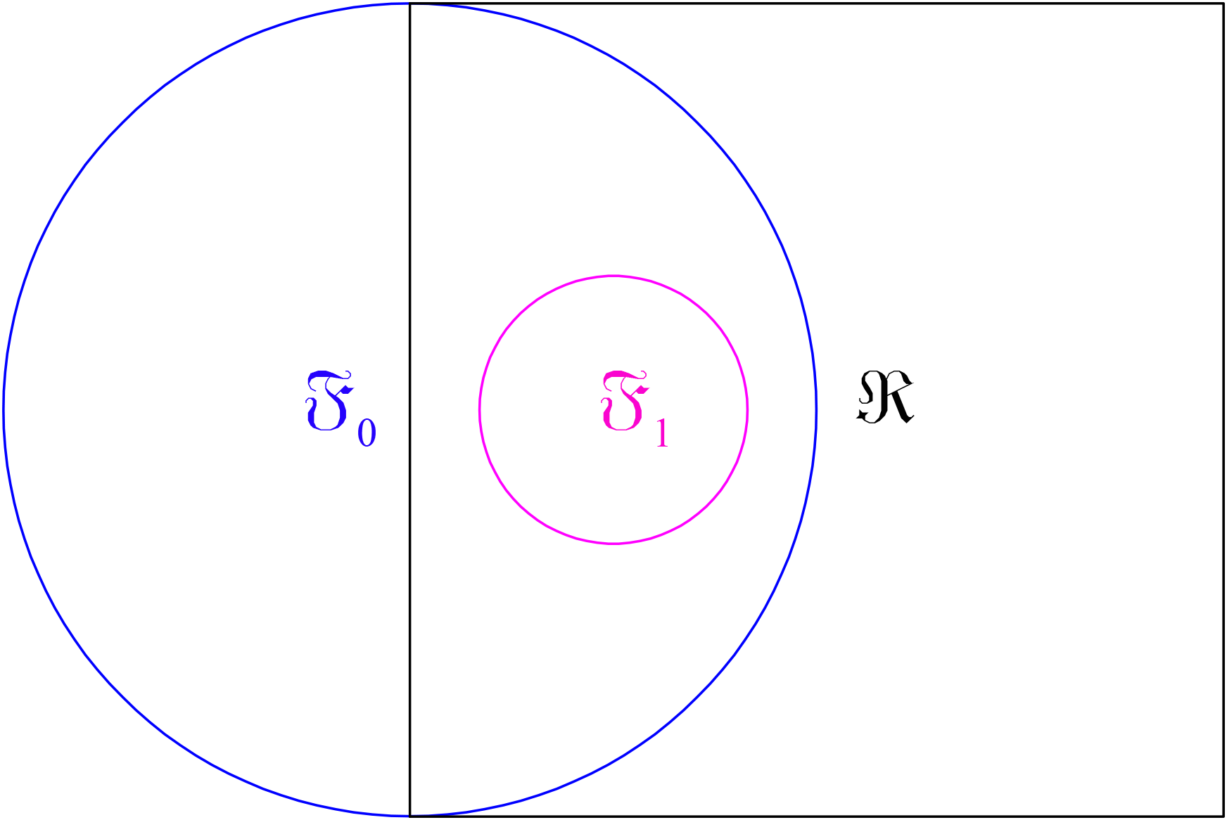
Figure 1: The three sets $\mathfrak{R},\mathfrak{F}_{0}$ and $\mathfrak{F}_{1}$.

For any $\varphi\in\mathfrak{F}_{1}$, using (4.7) and $\delta_{\lambda}\varphi(0)=\varphi(\lambda)$, we have

$$\tilde{F}_{\theta}[\varphi]\leq\mathbb{K}[\varphi],\text{ for }\varphi\in\mathfrak{F}_{1}.$$

By Hahn-Banach theorem, we extend the linear functional $\tilde{F}_{\theta}:\mathfrak{F}_{1}\rightarrow\mathbb{R}$ to $\tilde{F}_{\theta}:\mathfrak{R}\rightarrow\mathbb{R}$ such that $\tilde{F}_{\theta}[\varphi]\leq\mathbb{K}[\varphi]$ for $\varphi\in\mathfrak{R}$. Here we still use $\tilde{F}_{\theta}$ for notation simplicity. Since $\mathbb{K}[\cdot]$ is regular, it follows that $\tilde{F}_{\theta}$ is a positive linear functional satisfying $\tilde{F}_{\theta}[\varphi_{n}]\downarrow 0$ for each $\varphi_{n}\in\mathfrak{R}$ such that $\varphi_{n}\downarrow 0$. In turn, Daniell-Stone theorem implies that there exists a unique measure $v$ on $\big{(}\mathbb{R}^{d}\backslash\{0\},\mathcal{B}(\mathbb{R}^{d}\backslash\{0\})\big{)}$ such that

$$\tilde{F}_{\theta}[\varphi]=\int_{\mathbb{R}^{d}\backslash\{0\}}\varphi(z)v(dz)\text{, for }\varphi\in\mathfrak{R}.$$

We claim that there exists some $F_{\mu}\in\mathcal{L}$ such that

$$\tilde{F}_{\theta}[\varphi]=\int_{\mathbb{R}^{d}}\varphi(z)F_{\mu}(dz)\text{ , for }\varphi\in\mathfrak{R}.$$ (4.8)

Suppose not. For any $F_{\mu}\in\mathcal{L}$, there exists some $\varphi_{0}\in\mathfrak{R}$ such that

$$h(\varphi_{0},F_{\mu}):=\tilde{F}_{\theta}[\varphi_{0}]-\int_{\mathbb{R}^{d}}\varphi_{0}(z)F_{\mu}(dz)\neq 0.$$

Without loss of generality we may assume $h(\varphi_{0},F_{\mu})>0$. Since $k\varphi_{0}\in\mathfrak{R}$ for $k>0$, we show that for any $F_{\mu}\in\mathcal{L}$, $h(k\varphi_{0},F_{\mu})\rightarrow\infty$ as $k\rightarrow\infty$. Note that $\mathcal{L}$ is a compact convex set, it follows immediately from minimax theorem (cf. [10, 34]) that

$$\sup_{\varphi\in\mathfrak{R}}\inf_{F_{\mu}\in\mathcal{L}}h(\varphi,F_{\mu})=\inf_{F_{\mu}\in\mathcal{L}}\sup_{\varphi\in\mathfrak{R}}h(\varphi,F_{\mu})=\infty.$$

However, seeing that, $\tilde{F}_{\theta}[\varphi]-\mathbb{K}[\varphi]\leq 0$ for any $\varphi\in\mathfrak{R}$, then we have

$$\sup_{\varphi\in\mathfrak{R}}\inf_{F_{\mu}\in\mathcal{L}}h(\varphi,F_{\mu})\leq 0,$$

which induces a contradiction.

Step 3. For each $k>1$ and $i=1,\ldots,d$, We define $f_{k}^{i}(z)=(z_{i}\wedge k)\vee(-k)$ for $z=(z_{1},\ldots,z_{d})\in\mathbb{R}^{d}$. Let $f_{k}^{i,\varepsilon}(z):=\rho_{\varepsilon}\ast f_{k}^{i}(z)$, $i=1,\ldots,d$, be the smooth function with the mollifier $\rho_{\varepsilon}$ (see Appendix C.5 in [9]) and $f_{k}^{\varepsilon}:=(f_{k}^{1,\varepsilon},\ldots,f_{k}^{d,\varepsilon})$. Clearly, $f_{k}^{i,\varepsilon}\in\mathfrak{F}_{0}$, $Df_{k}^{i,\varepsilon}(0)=e_{i}$, where $e_{i}$ is the unit vector with the $i$th component 1, and

$$|f_{k}^{\varepsilon}(z)-z|\leq C|z|\mathbbm{1}_{\{|z|\geq k\}}\text{ \ with some }C>0.$$ (4.9)

Note that, for each $\varphi\in\mathfrak{F}_{0}$,

$$\tilde{F}_{\theta}[\varphi]=\tilde{F}_{\theta}[\varphi-\langle D\varphi(0),f_{k}^{\varepsilon}\rangle]+\tilde{F}_{\theta}[\langle D\varphi(0),f_{k}^{\varepsilon}\rangle].$$ (4.10)

Since $\varphi-\langle D\varphi(0),f_{k}^{\varepsilon}\rangle\in\mathfrak{F}_{1}$, from (4.8), we know that there exists some $F_{\mu}\in\mathcal{L}$ such that

$$\tilde{F}_{\theta}[\varphi-\langle D\varphi(0),f_{k}^{\varepsilon}\rangle]=\int_{\mathbb{R}^{d}}(\varphi(z)-\langle D\varphi(0),f_{k}^{\varepsilon}(z)\rangle)F_{\mu}(dz).$$

Besides, using (4.7) and (4.9), we derive that

$$\tilde{F}_{\theta}[\langle D\varphi(0),f_{k}^{\varepsilon}\rangle]\leq\sup\limits_{F_{\mu}\in\mathcal{L}}\int_{\mathbb{R}^{d}}\langle D\varphi(0),f_{k}^{\varepsilon}(z)-z\rangle F_{\mu}(dz)\leq C\sup\limits_{F_{\mu}\in\mathcal{L}}\int_{\{|z|\geq k\}}|z|F_{\mu}(dz)\rightarrow 0$$

as $k\rightarrow\infty$, and similarly, $\tilde{F}_{\theta}[\langle D\varphi(0),-f_{k}^{\varepsilon}\rangle]\rightarrow 0$ as $k\rightarrow\infty$. This implies that, $|\tilde{F}_{\theta}[\langle D\varphi(0),f_{k}^{\varepsilon}\rangle]|\rightarrow 0$ as $k\rightarrow\infty$. In addition, $\int_{\mathbb{R}^{d}}\langle D\varphi(0),z-f_{k}^{\varepsilon}\rangle F_{\mu}(dz)\rightarrow 0$ as $k\rightarrow\infty$. Therefore, by letting $k\rightarrow\infty$ in (4.10), we obtain that

$$\tilde{F}_{\theta}[\varphi]=\int_{\mathbb{R}^{d}}(\varphi(z)-\langle D\varphi(0),z\rangle)F_{\mu}(dz)\text{, for }\varphi\in\mathfrak{F}_{0}.$$ (4.11)

Together with (4.5)-(4.6), the conclusion follows.    

4.4 Connection to PIDE

In this section, we relate the nonlinear Lévy process $(\tilde{L}_{t})_{t\in[0,1]}$ to the fully nonlinear PIDE (3.3). Let $C_{b}^{2,3}([0,1]\times\mathbb{R}^{3d})$ denote the set of functions on $[0,1]\times\mathbb{R}^{3d}$ having bounded continuous partial derivatives up to the second order in $t$ and third order in $x,y,z$, respectively. Now we give the definition of viscosity solution for PIDE (3.3).

Definition 4.8

A bounded upper semicontinuous (resp. lower semicontinuous) function $u$ on $[0,1]\times\mathbb{R}^{3d}$ is called a viscosity subsolution (resp. viscosity supersolution) of (3.3) if $u(0,\cdot,\cdot,\cdot)\leq\phi(\cdot,\cdot,\cdot)$ $($resp. $\geq\phi(\cdot,\cdot,\cdot))$ and for each $(t,x,y,z)\in(0,1]\times\mathbb{R}^{3d}$,

$$\begin{array}[c]{l}\displaystyle\partial_{t}\psi(t,x,y,z)-\sup\limits_{(F_{\mu},q,Q)\in\Theta}\left\{\int_{\mathbb{R}^{d}}\delta_{\lambda}\psi(t,x,y,z)F_{\mu}(d\lambda)\right.\\ \displaystyle\text{\ \ \ \ \ \ \ \ \ \ \ \ \ \ \ }\left.+\langle D_{y}\psi(t,x,y,z),q\rangle+\frac{1}{2}tr[D_{x}^{2}\psi(t,x,y,z)Q]\text{ }\right\}\leq 0\text{ }(\text{resp. }\geq 0)\end{array}$$

whenever $\psi\in C_{b}^{2,3}((0,1]\times\mathbb{R}^{3d})$ is such that $\psi\geq u$ (resp. $\psi\leq u$) and $\psi(t,x,y,z)=u(t,x,y,z)$. A bounded continuous function $u$ is a viscosity solution of (3.3) if it is both a viscosity subsolution and supersolution.

For each $\phi\in C_{b,Lip}(\mathbb{R}^{3d})$, define

$$u(t,x,y,z)=\mathbb{\tilde{E}}[\phi(x+\tilde{\xi}_{t},y+\tilde{\eta}_{t},z+\tilde{\zeta}_{t})],\text{ }(t,x,y,z)\in[0,1]\times\mathbb{R}^{3d}.$$ (4.12)

Theorem 4.9

Suppose that assumptions (A1)-(A3) hold. Then, the value function $u$ of (4.12) is the unique viscosity solution of the fully nonlinear PIDE (3.3), i.e.,

$$\left\{\begin{array}[c]{l}\displaystyle\partial_{t}u(t,x,y,z)-\sup\limits_{(F_{\mu},q,Q)\in\Theta}\left\{\int_{\mathbb{R}^{d}}\delta_{\lambda}u(t,x,y,z)F_{\mu}(d\lambda)\right.\\ \displaystyle\text{\ \ \ \ \ \ \ \ \ \ \ \ \ \ \ }\left.+\langle D_{y}u(t,x,y,z),q\rangle+\frac{1}{2}tr[D_{x}^{2}u(t,x,y,z)Q]\right\}=0,\\ \displaystyle u(0,x,y,z)=\phi(x,y,z),\text{ \ }\forall(t,x,y,z)\in[0,1]\times\mathbb{R}^{3d},\end{array}\right.$$ (4.13)

where $\delta_{\lambda}u(t,x,y,z)=u(t,x,y,z+\lambda)-u(t,x,y,z)-\langle D_{z}u(t,x,y,z),\lambda\rangle$.

Proof. We first show that $u$ is continuous. It is clear that $u(t,\cdot,\cdot,\cdot)$ is uniformly Lipschitz continuous with the same Lipschitz constant as for $\phi$. For each $t,s\in[0,1]$ such that $t+s\leq 1$, we obtain

$$u(t+s,x,y,z)=\mathbb{\tilde{E}}[u(t,x+\tilde{\xi}_{s},y+\tilde{\eta}_{s},z+\tilde{\zeta}_{s})],\text{ \ }(x,y,z)\in\mathbb{R}^{3d},$$ (4.14)

which implies the continuity of $u(\cdot,x,y,z)$:

$$|u(t+s,x,y,z)-u(t,x,y,z)|\leq C\mathbb{\tilde{E}}[|\tilde{\xi}_{s}|+|\tilde{\eta}_{s}|+|\tilde{\zeta}_{s}|]\leq C\left(\sqrt{s}+s+M_{z}\sqrt[\alpha]{s}\right).$$

Next, we will prove that $u$ is the unique viscosity solution of (4.13). The uniqueness of viscosity solution can be found in Corollary 55 in [15]. It suffices to prove that $u$ is a viscosity subsolution, and the other case can be proved in a similar way. Assume that $\psi$ is a smooth test function on $(0,1]\times\mathbb{R}^{3d}$ satisfying $\psi\geq u$ and $\psi(\bar{t},\bar{x},\bar{y},\bar{z})=u(\bar{t},\bar{x},\bar{y},\bar{z})$ for some point $(\bar{t},\bar{x},\bar{y},\bar{z})\in(0,1]\times\mathbb{R}^{3d}$. For each $s\in(0,\bar{t})$, the dynamic programming principle (4.14) shows that

$$0 =\mathbb{\tilde{E}}[u(\bar{t}-s,\bar{x}+\tilde{\xi}_{s},\bar{y}+\tilde{\eta}_{s},\bar{z}+\tilde{\zeta}_{s})-u(\bar{t},\bar{x},\bar{y},\bar{z})]$$

$$\leq\mathbb{\tilde{E}}[\psi(\bar{t}-s,\bar{x}+\tilde{\xi}_{s},\bar{y}+\tilde{\eta}_{s},\bar{z}+\tilde{\zeta}_{s})-\psi(\bar{t},\bar{x},\bar{y},\bar{z})].$$

We claim that

$$\mathbb{\tilde{E}} [\psi(\bar{t}-s,\bar{x}+\tilde{\xi}_{s},\bar{y}+\tilde{\eta}_{s},\bar{z}+\tilde{\zeta}_{s})-\psi(\bar{t},\bar{x},\bar{y},\bar{z})]$$ (4.15)

$$=-\partial_{t}\psi(\bar{t},\bar{x},\bar{y},\bar{z})s+\mathbb{\tilde{E}}[\psi(\bar{t},\bar{x},\bar{y},\bar{z}+\tilde{\zeta}_{s})-\psi(\bar{t},\bar{x},\bar{y},\bar{z})$$

$$\text{ \ \ }+\langle D_{y}\psi(\bar{t},\bar{x},\bar{y},\bar{z}),\tilde{\eta}_{s}\rangle+\frac{1}{2}\langle D_{x}^{2}\psi(\bar{t},\bar{x},\bar{y},\bar{z})\tilde{\xi}_{s},\tilde{\xi}_{s}\rangle]+o(s),$$

whose proof will be given at the end of the proof. This implies that

$$0 \leq-\partial_{t}\psi(\bar{t},\bar{x},\bar{y},\bar{z})+\lim_{s\rightarrow 0}\mathbb{\tilde{E}}[\psi(\bar{t},\bar{x},\bar{y},\bar{z}+\tilde{\zeta}_{s})-\psi(\bar{t},\bar{x},\bar{y},\bar{z})$$ (4.16)

$$\text{ \ \ }+\langle D_{y}\psi(\bar{t},\bar{x},\bar{y},\bar{z}),\tilde{\eta}_{s}\rangle+\frac{1}{2}\langle D_{x}^{2}\psi(\bar{t},\bar{x},\bar{y},\bar{z})\tilde{\xi}_{s},\tilde{\xi}_{s}\rangle]s^{-1}.$$

In turn, Theorem 4.7 yields that there exists an uncertainty set $\Theta\subset\mathcal{L}\times\mathbb{R}^{d}\times\mathbb{S}_{+}(d)$ satisfying

$$\sup_{(F_{\mu},q,Q)\in\Theta}\left\{\int_{\mathbb{R}^{d}}|z|\wedge|z|^{2}F_{\mu}(dz)+|q|+|Q|\right\}<\infty$$

such that

$$\lim_{s\rightarrow 0}\mathbb{\tilde{E}}\big{[}\psi(\bar{t},\bar{x},\bar{y},\bar{z}+\tilde{\zeta}_{s})-\psi(\bar{t},\bar{x},\bar{y},\bar{z})+\langle D_{y}\psi(\bar{t},\bar{x},\bar{y},\bar{z}),\tilde{\eta}_{s}\rangle+\frac{1}{2}\langle D_{x}^{2}\psi(\bar{t},\bar{x},\bar{y},\bar{z})\tilde{\xi}_{s},\tilde{\xi}_{s}\rangle\big{]}s^{-1}$$ (4.17)

$$=\sup_{(F_{\mu},q,Q)\in\Theta}\left\{\int_{\mathbb{R}^{d}}\delta_{\lambda}\psi(\bar{t},\bar{x},\bar{y},\bar{z})F_{\mu}(d\lambda)+\langle D_{y}\psi(\bar{t},\bar{x},\bar{y},\bar{z}),q\rangle+\frac{1}{2}tr[D_{x}^{2}\psi(\bar{t},\bar{x},\bar{y},\bar{z})Q]\right\}.$$

Combining (4.16) with (4.17), it follows that

$$\displaystyle\partial_{t}\psi(\bar{t},\bar{x},\bar{y},\bar{z}) -\sup_{(F_{\mu},q,Q)\in\Theta}\left\{\int_{\mathbb{R}^{d}}\delta_{\lambda}\psi(\bar{t},\bar{x},\bar{y},\bar{z})F_{\mu}(d\lambda)\right.$$

$$\left.+\langle D_{y}\psi(\bar{t},\bar{x},\bar{y},\bar{z}),q\rangle+\frac{1}{2}tr[D_{x}^{2}\psi(\bar{t},\bar{x},\bar{y},\bar{z})Q]\right\}\leq 0,$$

which is the desired result.

We conclude the proof by showing (4.15). Note that

$$\psi(\bar{t}-s,\bar{x}+\tilde{\xi}_{s},\bar{y}+\tilde{\eta}_{s},\bar{z}+\tilde{\zeta}_{s})-\psi(\bar{t},\bar{x},\bar{y},\bar{z})$$

$$=\psi(\bar{t}-s,\bar{x}+\tilde{\xi}_{s},\bar{y}+\tilde{\eta}_{s},\bar{z}+\tilde{\zeta}_{s})-\psi(\bar{t},\bar{x}+\tilde{\xi}_{s},\bar{y}+\tilde{\eta}_{s},\bar{z}+\tilde{\zeta}_{s})$$ (4.18)

$$\text{ \ \ }+\psi(\bar{t},\bar{x}+\tilde{\xi}_{s},\bar{y}+\tilde{\eta}_{s},\bar{z}+\tilde{\zeta}_{s})-\psi(\bar{t},\bar{x},\bar{y},\bar{z}).$$

Taylor’s expansion yields that

$$\psi(\bar{t}-s,\bar{x}+\tilde{\xi}_{s},\bar{y}+\tilde{\eta}_{s},\bar{z}+\tilde{\zeta}_{s})-\psi(\bar{t},\bar{x}+\tilde{\xi}_{s},\bar{y}+\tilde{\eta}_{s},\bar{z}+\tilde{\zeta}_{s})=-\partial_{t}\psi(\bar{t},\bar{x},\bar{y},\bar{z})s+\epsilon_{1},$$ (4.19)

where

$$\epsilon_{1}=s\int_{0}^{1}\big{[}-\partial_{t}\psi(\bar{t}-\theta s,\bar{x}+\tilde{\xi}_{s},\bar{y}+\tilde{\eta}_{s},\bar{z}+\tilde{\zeta}_{s})+\partial_{t}\psi(\bar{t},\bar{x},\bar{y},\bar{z})\big{]}d\theta.$$

Since $\psi$ is the smooth function and $(\tilde{\xi}_{s},\tilde{\eta}_{s})$ $\overset{d}{=}(\sqrt{s}\tilde{\xi}_{1},s\tilde{\eta}_{1})$, we obtain that

$$\mathbb{\tilde{E}}[|\epsilon_{1}|]\leq C_{\psi}(s^{2}+\mathbb{\tilde{E}}[|\tilde{\xi}_{s}+\tilde{\eta}_{s}|]s+\mathbb{\tilde{E}}[|\tilde{\zeta}_{s}|]s)\leq Cs^{\frac{3}{2}}.$$

On the other hand, using Taylor’s expansion, we derive that

$$\psi(\bar{t},\bar{x}+\tilde{\xi}_{s},\bar{y}+\tilde{\eta}_{s},\bar{z}+\tilde{\zeta}_{s})-\psi(\bar{t},\bar{x},\bar{y},\bar{z})$$

$$=\psi(\bar{t},\bar{x},\bar{y},\bar{z}+\tilde{\zeta}_{s})-\psi(\bar{t},\bar{x},\bar{y},\bar{z})+\langle D_{x}\psi(\bar{t},\bar{x},\bar{y},\bar{z}),\tilde{\xi}_{s}\rangle$$ (4.20)

$$\text{ \ \ }+\langle D_{y}\psi(\bar{t},\bar{x},\bar{y},\bar{z}),\tilde{\eta}_{s}\rangle+\frac{1}{2}\langle D_{x}^{2}\psi(\bar{t},\bar{x},\bar{y},\bar{z})\tilde{\xi}_{s},\tilde{\xi}_{s}\rangle+\epsilon_{2},$$

where $\epsilon_{2}:=\epsilon_{2,1}+\epsilon_{2,2}$,

$$\epsilon_{2,1} =\psi(\bar{t},\bar{x}+\tilde{\xi}_{s},\bar{y}+\tilde{\eta}_{s},\bar{z}+\tilde{\zeta}_{s})-\psi(\bar{t},\bar{x},\bar{y},\bar{z}+\tilde{\zeta}_{s})$$

$$\text{ \ \ }-(\psi(\bar{t},\bar{x}+\tilde{\xi}_{s},\bar{y}+\tilde{\eta}_{s},\bar{z})-\psi(\bar{t},\bar{x},\bar{y},\bar{z}))$$

$$=\int_{0}^{1}\big{\langle}D_{x}\psi(\bar{t},\bar{x}+\theta\tilde{\xi}_{s},\bar{y}+\theta\tilde{\eta}_{s},\bar{z}+\tilde{\zeta}_{s})-D_{x}\psi(\bar{t},\bar{x}+\theta\tilde{\xi}_{s},\bar{y}+\theta\tilde{\eta}_{s},\bar{z}),\tilde{\xi}_{s}\big{\rangle}d\theta$$

$$\text{\ \ \ }+\int_{0}^{1}\big{\langle}D_{y}\psi(\bar{t},\bar{x}+\theta\tilde{\xi}_{s},\bar{y}+\theta\tilde{\eta}_{s},\bar{z}+\tilde{\zeta}_{s})-D_{y}\psi(\bar{t},\bar{x}+\theta\tilde{\xi}_{s},\bar{y}+\theta\tilde{\eta}_{s},\bar{z}),\tilde{\eta}_{s}\big{\rangle}d\theta$$

$$:=\int_{0}^{1}\big{\langle}\delta_{x}\psi(\tilde{\zeta}_{s};\bar{t},\bar{x}+\theta\tilde{\xi}_{s},\bar{y}+\theta\tilde{\eta}_{s}),\tilde{\xi}_{s}\big{\rangle}d\theta+\int_{0}^{1}\big{\langle}\delta_{y}\psi(\tilde{\zeta}_{s};\bar{t},\bar{x}+\theta\tilde{\xi}_{s},\bar{y}+\theta\tilde{\eta}_{s}),\tilde{\eta}_{s}\big{\rangle}d\theta$$

and

$$\epsilon_{2,2} =\psi(\bar{t},\bar{x}+\tilde{\xi}_{s},\bar{y}+\tilde{\eta}_{s},\bar{z})-\psi(\bar{t},\bar{x},\bar{y},\bar{z})-\langle D_{x}\psi(\bar{t},\bar{x},\bar{y},\bar{z}),\tilde{\xi}_{s}\rangle$$

$$\text{\ \ \ }-\langle D_{y}\psi(\bar{t},\bar{x},\bar{y},\bar{z}),\tilde{\eta}_{s}\rangle-\frac{1}{2}\langle D_{x}^{2}\psi(\bar{t},\bar{x},\bar{y},\bar{z})\tilde{\xi}_{s},\tilde{\xi}_{s}\rangle$$

$$=\int_{0}^{1}\int_{0}^{1}\big{\langle}(D_{x}^{2}\psi(\bar{t},\bar{x}+\tau\theta\tilde{\xi}_{s},\bar{y}+\tau\theta\tilde{\eta}_{s},\bar{z})-D_{x}^{2}\psi(\bar{t},\bar{x},\bar{y},\bar{z}))\tilde{\xi}_{s},\tilde{\xi}_{s}\big{\rangle}\theta d\theta d\tau$$

$$\text{\ \ \ }+\int_{0}^{1}\int_{0}^{1}\big{\langle}D_{y}^{2}\psi(\bar{t},\bar{x}+\tau\theta\tilde{\xi}_{s},\bar{y}+\tau\theta\tilde{\eta}_{s},\bar{z})\tilde{\eta}_{s},\tilde{\eta}_{s}\big{\rangle}\theta d\theta d\tau$$

$$\text{\ \ \ }+2\int_{0}^{1}\int_{0}^{1}\big{\langle}D_{xy}^{2}\psi(\bar{t},\bar{x}+\tau\theta\tilde{\xi}_{s},\bar{y}+\tau\theta\tilde{\eta}_{s},\bar{z})\tilde{\eta}_{s},\tilde{\xi}_{s}\big{\rangle}\theta d\theta d\tau.$$

Noting that $D\psi$ is bounded and choosing $p=\frac{2+\alpha}{2-\alpha}$ and $q=\frac{2+\alpha}{2\alpha}$, it follows that

$$\mathbb{\tilde{E}}[|\epsilon_{2,1}|] \leq\big{(}\mathbb{\tilde{E}}[|\tilde{\xi}_{s}|^{p}]\big{)}^{\frac{1}{p}}\bigg{(}\mathbb{\tilde{E}}\bigg{[}\int_{0}^{1}|\delta_{x}\psi(\tilde{\zeta}_{s};\bar{t},\bar{x}+\theta\tilde{\xi}_{s},\bar{y}+\theta\tilde{\eta}_{s})|^{q}d\theta\bigg{]}\bigg{)}^{\frac{1}{q}}$$

$$\text{ \ \ }+\big{(}\mathbb{\tilde{E}}[|\tilde{\eta}_{s}|^{p}]\big{)}^{\frac{1}{p}}\bigg{(}\mathbb{\tilde{E}}\bigg{[}\int_{0}^{1}|\delta_{y}\psi(\tilde{\zeta}_{s};\bar{t},\bar{x}+\theta\tilde{\xi}_{s},\bar{y}+\theta\tilde{\eta}_{s})|^{q}d\theta\bigg{]}\bigg{)}^{\frac{1}{q}}$$

$$\leq C\big{(}\mathbb{\tilde{E}}[|\tilde{\xi}_{s}|^{p}]\big{)}^{\frac{1}{p}}\bigg{(}\mathbb{\tilde{E}}\bigg{[}\int_{0}^{1}|\delta_{x}\psi(\tilde{\zeta}_{s};\bar{t},\bar{x}+\theta\tilde{\xi}_{s},\bar{y}+\theta\tilde{\eta}_{s})|d\theta\bigg{]}\bigg{)}^{\frac{1}{q}}$$

$$\text{ \ \ }+C\big{(}\mathbb{\tilde{E}}[|\tilde{\eta}_{s}|^{p}]\big{)}^{\frac{1}{p}}\bigg{(}\mathbb{\tilde{E}}\bigg{[}\int_{0}^{1}|\delta_{y}\psi(\tilde{\zeta}_{s};\bar{t},\bar{x}+\theta\tilde{\xi}_{s},\bar{y}+\theta\tilde{\eta}_{s})|d\theta\bigg{]}\bigg{)}^{\frac{1}{q}}$$

$$\leq C_{1}\Big{[}\big{(}\mathbb{\tilde{E}}[|\tilde{\xi}_{s}|^{p}]\big{)}^{\frac{1}{p}}+\big{(}\mathbb{\tilde{E}}[|\tilde{\eta}_{s}|^{p}]\big{)}^{\frac{1}{p}}\Big{]}\big{(}\mathbb{\tilde{E}}[|\tilde{\zeta}_{s}|]\big{)}^{\frac{1}{q}}=o(s).$$

Likewise, we have

$$\mathbb{\tilde{E}}[|\epsilon_{2,2}|]\leq C\mathbb{\tilde{E}}\big{[}|\tilde{\xi}_{s}|^{3}+|\tilde{\eta}_{s}||\tilde{\xi}_{s}|^{2}+|\tilde{\eta}_{s}|^{2}+2|\tilde{\eta}_{s}||\tilde{\xi}_{s}|\big{]}=o(s).$$

Consequently, together with (4.18)-(4.20) and $\mathbb{\tilde{E}}[\tilde{\xi}_{s}]=\mathbb{\tilde{E}}[-\tilde{\xi}_{s}]=0$, we prove (4.15). The proof is completed.    

5 An example

Example 5.1

This example illustrates the rationality of the conditions (A2)-(A3). For simplicity, we consider the case $d=2$. Given $\underline{\Lambda},\overline{\Lambda}>0$. Let $F_{\mu}$ be the Lévy measure given in Remark 3.3 with $\mu$ concentrated on the points $S_{0}=\{(1,0),(-1,0),(0,1),(0,-1)\}$,

$$\mathcal{L}_{0}=\left\{F_{\mu}\ \text{measure on }\mathbb{R}^{2}:\mu(\beta)\in(\underline{\Lambda},\overline{\Lambda}),\ \text{for }\beta\in S_{0}\right\},$$

and $\mathcal{L\subset L}_{0}$ be a nonempty compact convex set. Denote $K=(\underline{\Lambda},\overline{\Lambda})^{4}$ and

$$\begin{array}[c]{llll}k_{1}^{1}=\mu((-1,0)),&k_{2}^{1}=\mu((1,0)),&k_{1}^{2}=\mu((0,-1)),&k_{2}^{2}=\mu((0,1)).\end{array}$$

For each $(k_{1}^{1},k_{2}^{1},k_{1}^{2},k_{2}^{2})\in K$, let $W_{k^{i}}$, $i=1,2$, be two classical random variables such that for $i=1,2$,

(i)

$W_{k^{i}}$ has mean zero;

(ii)

$W_{k^{i}}$ has a cumulative distribution function

$$F_{W_{k^{i}}}(x)=\left\{\begin{array}[c]{ll}\displaystyle\left[k_{1}^{i}/\alpha+\beta_{1}^{i}(x)\right]\frac{1}{|x|^{\alpha}},&x<0,\\ \displaystyle 1-\left[k_{2}^{i}/\alpha+\beta_{2}^{i}(x)\right]\frac{1}{x^{\alpha}},&x>0,\end{array}\right.$$

with some continuously differentiable functions $\beta_{1}^{i}:$ $(-\infty,0]$ $\rightarrow\mathbb{R}$ and $\beta_{2}^{i}:[0,\infty)\rightarrow\mathbb{R}$ satisfying

$$\lim_{x\rightarrow-\infty}\beta_{1}^{i}(x)=\lim_{x\rightarrow\infty}\beta_{2}^{i}(x)=0.$$

(iii)

There exists a non-negative function $f$ on $\mathbb{N}$ tending to 0 as $n\rightarrow\infty$, such that the following quantities are less than $f(n)$ for all $n$:

$$\begin{array}[c]{lll}\displaystyle|\beta_{1}^{i}(-n^{1/\alpha})|,\text{ \ \ }&\displaystyle\int_{-\infty}^{-1}\frac{|\beta_{1}^{i}(n^{1/\alpha}x)|}{|x|^{\alpha}}dx,\text{ \ }&\displaystyle\int_{-1}^{0}\frac{|\beta_{1}^{i}(n^{1/\alpha}x)|}{|x|^{\alpha-1}}dx,\\ &&\\ \displaystyle|\beta_{2}^{i}(n^{1/\alpha})|,\text{ \ }&\displaystyle\int_{1}^{\infty}\frac{|\beta_{2}^{i}(n^{1/\alpha}x)|}{x^{\alpha}}dx,\text{ \ }&\displaystyle\int_{0}^{1}\frac{|\beta_{2}^{i}(n^{1/\alpha}x)|}{x^{\alpha-1}}dx.\end{array}$$

Denote $\tilde{\Omega}=\mathbb{R}^{2}$, $\mathcal{\tilde{H}}=C_{Lip}(\mathbb{R}^{2})$. For each $\chi=\varphi(x_{1},x_{2})\in\mathcal{\tilde{H}}$, define the sublinear expectation

$$\mathbb{\hat{E}}_{1}[\chi]=\sup_{(k_{1}^{1},k_{2}^{1},k_{1}^{2},k_{2}^{2})\in K}\int_{\mathbb{R}^{2}}\varphi(x_{1},x_{2})dF_{W_{k^{1}}}(x_{1})dF_{W_{k^{2}}}(x_{2}).$$

We consider an $\mathbb{R}^{2}$-valued random variable

$$Z(\tilde{\omega})=(Z^{1},Z^{2})(\tilde{\omega})=\tilde{\omega},\text{\ \ }\tilde{\omega}=(x_{1},x_{2})\in\tilde{\Omega}.$$

Clearly, $\mathbb{\hat{E}}_{1}[Z^{i}]=\mathbb{\hat{E}}_{1}[-Z^{i}]=0$ and $\mathbb{\hat{E}}_{1}[|Z^{i}|]<\infty$, for $i=1,2$. Construct a product space (cf. [31])

$$\big{(}\Omega,\mathcal{H},\mathbb{\hat{E}}\big{)}:=\big{(}\tilde{\Omega}^{\mathbb{N}},\tilde{\mathcal{H}}^{\otimes^{\mathbb{N}}},\mathbb{\hat{E}}_{1}^{\otimes^{\mathbb{N}}}\big{)}$$

and introduce $Z_{i}(\omega):=Z(\tilde{\omega}_{i})$, for $\omega=(\tilde{\omega}_{1},\tilde{\omega}_{2,}\cdots)\in\Omega$, $i=1,2,\cdots$. Then $\{Z_{i}\}_{i=1}^{\infty}$ be a sequence of i.i.d. $\mathbb{R}^{2}$-valued random variables on $\big{(}\Omega,\mathcal{H},\mathbb{\hat{E}}\big{)}$ in the sense that $Z_{i+1}\overset{d}{=}Z_{i}$, and $Z_{i+1}\perp\!\!\!\perp(Z_{1},Z_{2},\ldots,Z_{i})$ for each $i\in\mathbb{N}$.

Next, we shall adapt the method developed in [13] to prove $M_{z}<\infty$. For given $n$, define an approximation scheme $u_{n}:[0,1]\times\mathbb{R}^{2}\rightarrow\mathbb{R}$ recursively by

$$\begin{array}[c]{l}u_{n}(t,z)=|z|,\text{ \ if }t\in[0,1/n),\\ u_{n}(t,z)=\mathbb{\hat{E}}[u_{n}(t-1/n,z+n^{-1/\alpha}Z)]\text{, \ if }t\in[1/n,1].\end{array}$$

Then, $u_{n}(1,0)=n^{-\frac{1}{\alpha}}\mathbb{\hat{E}}[|S_{n}^{3}|]$. By means of Theorem 4.1 in [13], we get

$$u_{n}(1,0)=u_{n}(1,0)-u_{n}(0,0)\leq C(1+\sqrt{f(n)})$$

approaches $C<\infty$ as $n\rightarrow\infty$, which implies (A2) holds.

To verify (A3), we further impose the condition

(iv)

There exists a constant $M>0$ such that for any $(k_{1}^{1},k_{2}^{1},k_{1}^{2},k_{2}^{2})\in K$, the following quantities are less than $M$:

$$\begin{array}[c]{lll}\displaystyle\left|\int_{-\infty}^{-1}\frac{\beta_{1}^{i}(x)}{|x|^{\alpha}}dx\right|,\text{\ }&&\displaystyle\left|\int_{1}^{\infty}\frac{\beta_{2}^{i}(x)}{x^{\alpha}}dx\right|.\end{array}$$

Following along similar arguments as in Remark 3.3, we derive that for $\varphi\in C_{b}^{3}(\mathbb{R}^{2})$

$$\frac{1}{s}\bigg{|}\mathbb{\hat{E}}\big{[}\varphi(z+s^{\frac{1}{\alpha}}Z_{1})-\varphi(z)\big{]}-s\sup_{F_{\mu}\in\mathcal{L}}\int_{\mathbb{R}^{2}}\delta_{\lambda}\varphi(z)F_{\mu}(d\lambda)\bigg{|}$$

$$\leq\frac{1}{s}\mathbb{\hat{E}}\bigg{[}\bigg{|}\mathbb{\hat{E}}\big{[}\delta_{s^{1/\alpha}Z_{1}^{1}}^{1}\varphi(z_{1},z_{2}+x_{2})\big{]}-s\sup_{F_{\mu}\in\mathcal{L}}\int_{\mathbb{R}}\delta_{\lambda_{1}}^{1}\varphi(z_{1},z_{2}+x_{2})F_{\mu}^{1}(d\lambda_{1})\bigg{|}_{x_{2}=s^{1/\alpha}Z_{1}^{2}}\bigg{]}$$

$$\text{ \ \ }+Cs^{\frac{1}{\alpha}}\mathbb{\hat{E}}[|Z_{1}^{2}|]+\frac{1}{s}\bigg{|}\mathbb{\hat{E}}\big{[}\delta_{s^{1/\alpha}Z_{1}^{2}}^{2}\varphi(z_{1},z_{2})\big{]}-s\sup_{F_{\mu}\in\mathcal{L}}\int_{\mathbb{R}}\delta_{\lambda_{2}}^{2}\varphi(z_{1},z_{2})F_{\mu}^{2}(d\lambda_{2})\bigg{|}\rightarrow 0$$

uniformly on $z\in\mathbb{R}^{2}$ as $s\rightarrow 0$.

6 Appendix

6.1 Proof of Theorem 2.9

Since sublinear expectations $\{\mathbb{\hat{E}}_{\alpha}\}_{\alpha\in\mathcal{A}}$ are tight on $(\mathbb{R}^{n},C_{b,Lip}(\mathbb{R}^{n}))$, then there exists a tight sublinear expectation $\mathbb{\hat{E}}$ on $(\mathbb{R}^{n},C_{b,Lip}(\mathbb{R}^{n}))$ such that

$$\mathbb{\hat{E}}_{\alpha}[\varphi]-\mathbb{\hat{E}}_{\alpha}[\varphi^{\prime}]\leq\mathbb{\hat{E}}[\varphi-\varphi^{\prime}],\text{ for each }\varphi,\varphi^{\prime}\in C_{b,Lip}(\mathbb{R}^{n}).$$

Let $\{N_{i}\}_{i=1}^{\infty}$ be a sequence of strictly increasing positive integers satisfying for each $i\in\mathbb{N}$ there exists a $\phi_{i}\in C_{b,Lip}(\mathbb{R}^{n})$ with $\mathbbm{1}_{\{|x|\geq N_{i}\}}\leq\phi_{i}$ such that $\mathbb{\hat{E}}[\phi_{i}]\leq 1/i$. Denote $K_{i}:=\{|x|\leq N_{i}\}$ for $i\in\mathbb{N}$. Let $\{\varphi_{j}\}_{j=1}^{\infty}$ constitute a linear subspace of $C_{b,Lip}(\mathbb{R}^{n})$ such that for each $K_{i}$, $\{\varphi_{j}(x)\}_{j=1}^{\infty}|_{x\in K_{i}}$ is dense in $C_{b,Lip}(K_{i})$.

We first claim that there exists a subsequence $\{\mathbb{\hat{E}}_{\alpha_{n_{i}}}\}_{i=1}^{\infty}$ such that, for each $j\in\mathbb{N}$, $\{\mathbb{\hat{E}}_{\alpha_{n_{i}}}[\varphi_{j}]\}_{i=1}^{\infty}$ is a Cauchy sequence. Indeed, note that $\{\mathbb{\hat{E}}_{\alpha_{n}}[\varphi_{1}]\}_{n=1}^{\infty}$ is a bounded sequence, then there exists a subsequence $\{\mathbb{\hat{E}}_{\alpha_{n_{1}(i)}}\}_{i=1}^{\infty}\subset\{\mathbb{\hat{E}}_{\alpha_{n}}\}_{n=1}^{\infty}$ such that $\{\mathbb{\hat{E}}_{\alpha_{n_{1}(i)}}[\varphi_{1}]\}_{i=1}^{\infty}$ is a Cauchy sequence. Similar procedure applies to $\{\mathbb{\hat{E}}_{\alpha_{n_{1}(i)}}[\varphi_{2}]\}_{i=1}^{\infty}$, we find a subsequence $\{\mathbb{\hat{E}}_{\alpha_{n_{2}(i)}}\}_{i=1}^{\infty}\subset\{\mathbb{\hat{E}}_{\alpha_{n_{1}(i)}}\}_{i=1}^{\infty}$ such that $\{\mathbb{\hat{E}}_{\alpha_{n_{2}(i)}}[\varphi_{2}]\}_{i=1}^{\infty}$ is a Cauchy sequence. Repeating this process, we find that, for each $j\in\mathbb{N}$, a subsequence $\{\mathbb{\hat{E}}_{\alpha_{n_{j}(i)}}\}_{i=1}^{\infty}\subset\{\mathbb{\hat{E}}_{\alpha_{n_{j-1}(i)}}\}_{i=1}^{\infty}$ such that $\{\mathbb{\hat{E}}_{\alpha_{n_{j}(i)}}[\varphi_{j}]\}_{i=1}^{\infty}$ is a Cauchy sequence. Taking the diagonal sequence $\{\mathbb{\hat{E}}_{\alpha_{n_{i}(i)}}\}_{i=1}^{\infty}$, then for each $j\in\mathbb{N}$, $\{\mathbb{\hat{E}}_{\alpha_{n_{i}(i)}}[\varphi_{j}]\}_{i=1}^{\infty}$ is a Cauchy sequence. Thus, the claim follows by letting $n_{i}=n_{i}(i)$.

It remains prove that for each $\varphi\in C_{b,Lip}(\mathbb{R}^{n})$, $\{\mathbb{\hat{E}}_{\alpha_{n_{i}}}[\varphi]\}_{i=1}^{\infty}$ is also a Cauchy sequence. Denote $M:=\sup_{x\in\mathbb{R}^{n}}|\varphi(x)|$. For each $\varepsilon>0$, we choose some $m>16M/\varepsilon$ such that $\mathbbm{1}_{\{|x|\geq N_{m}\}}\leq\phi_{m}$ and $\mathbb{\hat{E}}[\phi_{m}]\leq\frac{\varepsilon}{16M}$. Let $\{\varphi_{j_{l}}\}_{l=1}^{\infty}$ be a subsequence of $\{\varphi_{j}\}_{j=1}^{\infty}$ such that $\sup\limits_{l\in\mathbb{N}}\sup\limits_{x\in\mathbb{R}^{n}}|\varphi_{j_{l}}(x)|\leq M$ and

$$\lim\limits_{l\rightarrow\infty}\sup\limits_{x\in K_{m}}|\varphi_{j_{l}}(x)-\varphi(x)|=0,$$

Thus there exists some large integer $l_{0}$ such that $\sup\limits_{x\in K_{m}}|\varphi_{j_{l_{0}}}(x)-\varphi(x)|\leq\varepsilon/8$, which implies that for $x\in\mathbb{R}^{n}$

$$|\varphi_{j_{l_{0}}}(x)-\varphi(x)| =|\varphi_{j_{l_{0}}}(x)-\varphi(x)|\mathbbm{1}_{K_{m}}(x)+|\varphi_{j_{l_{0}}}(x)-\varphi(x)|\mathbbm{1}_{K_{m}^{c}}(x)$$

$$\leq\sup\limits_{y\in K_{m}}|\varphi_{j_{l_{0}}}(y)-\varphi(y)|\mathbbm{1}_{K_{m}}(x)+2M\mathbbm{1}_{\{|x|\geq N_{m}\}}$$

$$\leq\varepsilon/8+2M\phi_{m}(x).$$

Then one easily gets $\mathbb{\hat{E}}\big{[}|\varphi_{j_{l_{0}}}-\varphi|\big{]}\leq\varepsilon/4$. For this $l_{0}$, we know that there exist a large integer $i_{0}$, such that $\big{|}\mathbb{\hat{E}}_{\alpha_{n_{i}}}[\varphi_{j_{l_{0}}}]-\mathbb{\hat{E}}_{\alpha_{n_{j}}}[\varphi_{j_{l_{0}}}]\big{|}\leq\varepsilon/2$ for any $i,j\geq i_{0}$. Then, it follows that

$$\big{|}\mathbb{\hat{E}}_{\alpha_{n_{i}}}[\varphi]-\mathbb{\hat{E}}_{\alpha_{n_{j}}}[\varphi]\big{|}\leq 2\mathbb{\hat{E}}\big{[}|\varphi-\varphi_{j_{l_{0}}}|\big{]}+\big{|}\mathbb{\hat{E}}_{\alpha_{n_{i}}}[\varphi_{j_{l_{0}}}]-\mathbb{\hat{E}}_{\alpha_{n_{j}}}[\varphi_{j_{l_{0}}}]\big{|}\leq\varepsilon.$$

Therefore, we conclude that $\{\mathbb{\hat{E}}_{\alpha_{n_{i}}}[\varphi]\}_{i=1}^{\infty}$ is a Cauchy sequence. This completes the proof.

6.2 The construction of nonlinear Lévy process $(\tilde{L}_{t})_{t\in[0,1]}$

In the following, we will construct a sublinear expectation $\mathbb{\tilde{E}}:Lip(\tilde{\Omega})\rightarrow\mathbb{R}$ such that the canonical process $(\tilde{L}_{t})_{t\in[0,1]}$ is a nonlinear Lévy process. We divide it into the following three steps.

Step 1. For each $m\geq 0$, let $\tau_{m}=2^{-m}$,

$$\begin{array}[c]{l}\displaystyle\mathcal{H}^{m}=\big{\{}\varphi\big{(}\tilde{L}_{\tau_{m}},\tilde{L}_{2\tau_{m}}-\tilde{L}_{\tau_{m}},\ldots,\tilde{L}_{2^{m}\tau_{m}}-\tilde{L}_{(2^{m}-1)\tau_{m}}\big{)}:\forall\varphi\in C_{b,Lip}\big{(}\mathbb{R}^{2^{m}\times 3d}\big{)}\big{\}}\text{, \ for }m\geq 1,\\ \displaystyle\mathcal{H}^{0}=\big{\{}\phi\big{(}\tilde{L}_{1}\big{)}:\forall\phi\in C_{b,Lip}\big{(}\mathbb{R}^{3d}\big{)}\big{\}}.\end{array}$$

Let $\{L_{\tau_{m}}^{n}\}_{n=1}^{\infty}$ be a sequence of i.i.d. $\mathbb{R}^{3d}$-valued random variables defined on $(\Omega,\mathcal{H},\mathbb{\hat{E}}_{1})$ in the sense that $L_{\tau_{m}}^{1}\overset{d}{=}L_{\tau_{m}}$, $L_{\tau_{m}}^{n+1}\overset{d}{=}L_{\tau_{m}}^{n}$ and $L_{\tau_{m}}^{n+1}\perp\!\!\!\perp(L_{\tau_{m}}^{1},L_{\tau_{m}}^{2},\ldots,L_{\tau_{m}}^{n})$ for each $n\in\mathbb{N}$. For given $m\geq 1$, $\phi\big{(}\tilde{L}_{n\tau_{m}}-\tilde{L}_{(n-1)\tau_{m}}\big{)}$ with $1\leq n\leq 2^{m}$, and $\phi\in C_{b,Lip}(\mathbb{R}^{3d})$, define

$$\mathbb{\tilde{E}}^{m}\big{[}\phi\big{(}\tilde{L}_{n\tau_{m}}-\tilde{L}_{(n-1)\tau_{m}}\big{)}\big{]}=\mathbb{\hat{E}}_{1}\big{[}\phi(L_{\tau_{m}}^{n})\big{]}.$$

For $\varphi\big{(}\tilde{L}_{\tau_{m}},\ldots,\tilde{L}_{2^{m}\tau_{m}}-\tilde{L}_{(2^{m}-1)\tau_{m}}\big{)}\in\mathcal{H}^{m}$, for some $\varphi\in C_{b,Lip}\big{(}\mathbb{R}^{2^{m}\times 3d}\big{)}$, define

$$\mathbb{\tilde{E}}^{m}\big{[}\varphi\big{(}\tilde{L}_{\tau_{m}},\ldots,\tilde{L}_{2^{m}\tau_{m}}-\tilde{L}_{(2^{m}-1)\tau_{m}}\big{)}\big{]}=\varphi_{0},$$

where $\varphi_{0}$ is defined iteratively through

$$\begin{array}[c]{c}\displaystyle\varphi_{2^{m}-1}(x_{1},x_{2},\ldots,x_{2^{m}-1})=\mathbb{\tilde{E}}^{m}\big{[}\varphi\big{(}x_{1},x_{2},\ldots,x_{2^{m}-1},\tilde{L}_{2^{m}\tau_{m}}-\tilde{L}_{(2^{m}-1)\tau_{m}}\big{)}\big{]}\\ \displaystyle\varphi_{2^{m}-2}(x_{1},x_{2},\ldots,x_{2^{m}-2})=\mathbb{\tilde{E}}^{m}\big{[}\varphi_{2^{m}-1}\big{(}x_{1},x_{2},\ldots,x_{2^{m}-2},\tilde{L}_{(2^{m}-1)\tau_{m}}-\tilde{L}_{(2^{m}-2)\tau_{m}}\big{)}\big{]}\\ \displaystyle\vdots\\ \displaystyle\varphi_{1}(x_{1})=\mathbb{\tilde{E}}^{m}\big{[}\varphi_{2}\big{(}x_{1},\tilde{L}_{2\tau_{m}}-\tilde{L}_{\tau_{m}}\big{)}\big{]}\\ \displaystyle\varphi_{0}=\mathbb{\tilde{E}}^{m}\big{[}\varphi_{1}\big{(}\tilde{L}_{\tau_{m}}\big{)}\big{]}.\end{array}$$

For $\phi\in C_{b,Lip}(\mathbb{R}^{3d})$, we also define

$$\mathbb{\tilde{E}}^{0}\big{[}\phi\big{(}\tilde{L}_{1}\big{)}\big{]}=\mathbb{\hat{E}}_{1}\big{[}\phi(L_{1})\big{]}.$$

From the above definition we know that $(\tilde{\Omega},\mathcal{H}^{m},\mathbb{\tilde{E}}^{m})$ is a sublinear expectation space under which $\tilde{L}_{t}-\tilde{L}_{s}\overset{d}{=}$ $\tilde{L}_{t-s}$ and $\tilde{L}_{t}-\tilde{L}_{s}\perp\!\!\!\perp(\tilde{L}_{t_{1}},\ldots,\tilde{L}_{t_{i}})$ for each $t_{i},s,t\in\mathcal{D}_{m}[0,1]:=\{l2^{-m}:0\leq l\leq 2^{m},l\in\mathbb{N}\}$ with $t_{i}\leq s\leq t$. Also, it can be checked that $\mathbb{\tilde{E}}^{m}[\cdot]$ is consistent, i.e., for each $m\geq 0$, $\mathbb{\tilde{E}}^{m+1}[\cdot]=\mathbb{\tilde{E}}^{m}[\cdot]$ on $\mathcal{H}^{m}$.

Step 2. Note that $\mathcal{H}^{m}\subset\mathcal{H}^{m+1}$, for each $m\geq 0$. Denote

$$\mathcal{H}^{\infty}=\bigcup_{m\geq 0}\mathcal{H}^{m}.$$

Obviously, $\mathcal{H}^{\infty}\subset Lip(\tilde{\Omega})$ such that if $\chi_{1},\cdots,\chi_{i}\in\mathcal{H}^{\infty}$, then $\varphi(\chi_{1},\cdots,\chi_{i})\in\mathcal{H}^{\infty}$ for $\varphi\in C_{b,Lip}(\mathbb{R}^{i})$. For any $\chi\in\mathcal{H}^{\infty}$, there exists an $m_{0}\in\mathbb{N}$ such that $\chi\in\mathcal{H}^{m_{0}}$, define

$$\mathbb{\tilde{E}}[\chi]:=\mathbb{\tilde{E}}^{m_{0}}[\chi].$$

Since $\mathbb{\tilde{E}}^{m}[\cdot]$ is consistent, $\mathbb{\tilde{E}}:\mathcal{H}^{\infty}\rightarrow\mathbb{R}$ is a well-defined sublinear expectation.

Step 3. We extend the sublinear expectation $\mathbb{\tilde{E}}:\mathcal{H}^{\infty}\rightarrow\mathbb{R}$ to $\mathbb{\tilde{E}}:Lip(\tilde{\Omega})\rightarrow\mathbb{R}$ and still use $\mathbb{\tilde{E}}$ for simplicity. Denote $\mathcal{D}_{\infty}[0,1]:=\cup_{m\geq 0}\mathcal{D}_{m}[0,1]$. For each $\varphi(\tilde{L}_{t_{1}},\ldots,\tilde{L}_{t_{n}}-\tilde{L}_{t_{n-1}})\in Lip(\tilde{\Omega})$ with $\varphi\in C_{b,Lip}(\mathbb{R}^{n\times 3d})$, for each $t_{k}\in[0,1]$, $1\leq k\leq n$, we choose a sequence $\{t_{k}^{i}\}_{i=1}^{\infty}\in\mathcal{D}_{\infty}[0,1]$ such that $t_{k}^{i}<t_{k+1}^{i}$ and $t_{k}^{i}\downarrow t_{k}$ as $i\rightarrow\infty$. Define

$$\mathbb{\tilde{E}}\big{[}\varphi\big{(}\tilde{L}_{t_{1}},\ldots,\tilde{L}_{t_{n}}-\tilde{L}_{t_{n-1}}\big{)}\big{]}=\lim_{i\rightarrow\infty}\mathbb{\tilde{E}}\big{[}\varphi\big{(}\tilde{L}_{t_{1}^{i}},\ldots,\tilde{L}_{t_{n}^{i}}-\tilde{L}_{t_{n-1}^{i}}\big{)}\big{]}.$$

It can be verified that the limit does not depend on the choice of $\{t_{k}^{i}\}_{i=1}^{\infty}$. Indeed, for two descending sequences $\{t_{k}^{i}\}_{i=1}^{\infty}$ and $\{t_{k}^{i^{\prime}}\}_{i^{\prime}=1}^{\infty}$ with the same limit $t_{k}$ as $i,i^{\prime}\rightarrow\infty$, we assume that $t_{k}^{i}-t_{k}^{i^{\prime}}:=l_{k}\tau_{m_{k}}$ for some $m_{k}\in\mathbb{N}$ and $1\leq l_{k}\leq 2^{m_{k}}$. From the construction of $\tilde{L}_{\cdot}$ and Remark 2.13, there exists a convergent sequence $\{\bar{S}_{n_{j}^{\ast}}^{\tau_{m_{k}}}\}_{j=1}^{\infty}$ such that for $\varphi\in C_{b,Lip}(\mathbb{R}^{n\times 3d})$

$$\begin{array}[c]{l}\displaystyle\left|\mathbb{\tilde{E}}\big{[}\varphi\big{(}\tilde{L}_{t_{1}^{i}},\ldots,\tilde{L}_{t_{n}^{i}}-\tilde{L}_{t_{n-1}^{i}}\big{)}\big{]}-\mathbb{\tilde{E}}\big{[}\varphi\big{(}\tilde{L}_{t_{1}^{i^{\prime}}},\ldots,\tilde{L}_{t_{n}^{i^{\prime}}}-\tilde{L}_{t_{n-1}^{i^{\prime}}}\big{)}\big{]}\right|\\ \displaystyle\leq L_{\varphi}\mathbb{\tilde{E}}\big{[}\big{(}\sum_{k=1}^{n}|\tilde{L}_{t_{k}^{i}}-\tilde{L}_{t_{k-1}^{i}}-\tilde{L}_{t_{k}^{i^{\prime}}}+\tilde{L}_{t_{k-1}^{i^{\prime}}}|\big{)}\wedge 2N_{\varphi}\big{]}\\ \displaystyle\leq 2L_{\varphi}\sum_{k=1}^{n}\mathbb{\tilde{E}}\big{[}|\tilde{L}_{t_{k}^{i}-t_{k}^{i^{\prime}}}|\wedge 2N_{\varphi}\big{]}\\ \displaystyle=2L_{\varphi}\sum\limits_{k=1}^{n}\mathbb{\hat{E}}_{1}\big{[}|L_{\tau_{m_{k}}}^{1}+\cdots+L_{\tau_{m_{k}}}^{l_{k}}|\wedge 2N_{\varphi}\big{]}\\ \displaystyle=2L_{\varphi}\sum_{k=1}^{n}\lim\limits_{j\rightarrow\infty}\mathbb{\hat{E}}\big{[}|\bar{S}_{l_{k}n_{j}^{\ast}}^{t_{k}^{i}-t_{k}^{i^{\prime}}}|\wedge 2N_{\varphi}\big{]}\\ \displaystyle\leq 2L_{\varphi}\sum_{k=1}^{n}\lim\limits_{j\rightarrow\infty}\mathbb{\hat{E}}\big{[}\big{|}(t_{k}^{i}-t_{k}^{i^{\prime}})^{1/2}(l_{k}n_{j}^{\ast})^{-1/2}S_{l_{k}n_{j}^{\ast}}^{1}\big{|}\wedge 2N_{\varphi}\big{]}\\ \displaystyle\text{ \ \ }+2L_{\varphi}\sum_{k=1}^{n}\lim\limits_{j\rightarrow\infty}\mathbb{\hat{E}}\big{[}\big{|}(t_{k}^{i}-t_{k}^{i^{\prime}})(l_{k}n_{j}^{\ast})^{-1}S_{l_{k}n_{j}^{\ast}}^{2}\big{|}\wedge 2N_{\varphi}\big{]}\\ \displaystyle\text{ \ \ }+2L_{\varphi}\sum_{k=1}^{n}\lim\limits_{j\rightarrow\infty}\mathbb{\hat{E}}\big{[}\big{|}(t_{k}^{i}-t_{k}^{i^{\prime}})^{1/\alpha}(l_{k}n_{j}^{\ast})^{-1/\alpha}S_{l_{k}n_{j}^{\ast}}^{3}\big{|}\wedge 2N_{\varphi}\big{]}\\ \displaystyle\leq 2L_{\varphi}\sum_{k=1}^{n}\mathbb{\hat{E}}_{1}\big{[}\big{(}|t_{k}^{i}-t_{k}^{i^{\prime}}|^{1/2}|\xi_{1}|\big{)}\wedge 2N_{\varphi}\big{]}\\ \displaystyle\text{ \ \ }+2L_{\varphi}\sum_{k=1}^{n}\mathbb{\hat{E}}_{1}\big{[}\big{(}|t_{k}^{i}-t_{k}^{i^{\prime}}||\eta_{1}|\big{)}\wedge 2N_{\varphi}\big{]}+2L_{\varphi}M_{z}\sum_{k=1}^{n}|t_{k}^{i}-t_{k}^{i^{\prime}}|^{1/\alpha}\\ \displaystyle\rightarrow 0\text{, \ as }i,i^{\prime}\rightarrow\infty,\end{array}$$

where $L_{\varphi}>0$ is the Lipschitz constant of $\varphi$, $K_{\varphi}:=|\varphi|_{0}$ and $N_{\varphi}:=\frac{K_{\varphi}}{L_{\varphi}}$. Also, $\mathbb{\tilde{E}}:Lip(\tilde{\Omega})\rightarrow\mathbb{R}$ is a well-defined sublinear expectation, that is, if $\varphi(\tilde{L}_{t_{1}},\ldots,$ $\tilde{L}_{t_{n}}-\tilde{L}_{t_{n-1}})=\varphi^{\prime}(\tilde{L}_{t_{1}},\ldots,\tilde{L}_{t_{n}}-\tilde{L}_{t_{n-1}})$ with $\varphi,\varphi^{\prime}\in C_{b,Lip}(\mathbb{R}^{n\times 3d})$, then

$$\mathbb{\tilde{E}}\big{[}\varphi\big{(}\tilde{L}_{t_{1}},\ldots,\tilde{L}_{t_{n}}-\tilde{L}_{t_{n-1}}\big{)}\big{]}=\mathbb{\tilde{E}}\big{[}\varphi^{\prime}\big{(}\tilde{L}_{t_{1}},\ldots,\tilde{L}_{t_{n}}-\tilde{L}_{t_{n-1}}\big{)}\big{]}.$$

Moreover, for each $t_{i},s,t\in[0,1]\$with $t_{i}\leq s\leq t$, $\tilde{L}_{t}-\tilde{L}_{s}\overset{d}{=}$ $\tilde{L}_{t-s}$ and $\tilde{L}_{t}-\tilde{L}_{s}\perp\!\!\!\perp(\tilde{L}_{t_{1}},\ldots,\tilde{L}_{t_{i}})$ under $\mathbb{\tilde{E}}$. Thus, $(\tilde{\Omega},Lip(\tilde{\Omega}),\mathbb{\tilde{E}})$ is a sublinear expectation space on which the canonical process $(\tilde{L}_{t})_{t\in[0,1]}$ is a nonlinear Lévy process.

References

- [1] G. Barles and E. R. Jakobsen, On the convergence rate of approximation schemes for Hamilton-Jacobi-Bellman equations, M2AN Math. Model. Numer. Anal., 36 (2002), pp. 33-54.
- [2] G. Barles and E. R. Jakobsen, Error bounds for monotone approximation schemes for Hamilton-Jacobi-Bellman equations, SIAM J. Numer. Anal., 43 (2005), pp. 540-558.
- [3] G. Barles and E. R. Jakobsen, Error bounds for monotone approximation schemes for parabolic Hamilton-Jacobi-Bellman equations. Mathematics of Computation, 76 (2007), pp. 1861-1893.
- [4] G. Barles and P. E. Souganidis, Convergence of approximation schemes for fully nonlinear second order equations, Asymptotic Analysis, 4 (1991), pp. 271-283.
- [5] E. Bayraktar and A. Munk, An -stable limit theorem under sublinear expectation, Bernoulli, 22 (2016), pp. 2548-2578.
- [6] L. A. Caffarelli and X. Cabré, Fully nonlinear elliptic equations, American Mathematical Society, Providence, RI, 1995.
- [7] Z. Chen, Strong laws of large numbers for sub-linear expectations, Sci. China Math., 59 (2016), pp. 945-954.
- [8] R. Denk, M. Kupper, and M. Nendel, A semigroup approach to nonlinear Lévy processes, Stochastic Process. Appl., 130 (2020), pp.1616-1642.
- [9] L. C. Evans, Partial differential equations, American Mathematical Soc., 2010.
- [10] K. Fan, Minimax theorems, Proc. Nat. Acad. Sci. USA, 39 (1953), pp. 42-47.
- [11] X. Fang, S. Peng, Q. Shao, and Y. Song, Limit theorem with rate of convergence under sublinear expectations, Bernoulli, 25 (2019), pp. 2564-2596.
- [12] X. Guo and X. Li, On the laws of large numbers for pseudo-independent random variables under sublinear expectation, Statistics & Probability Letters, 172 (2021), 109042.
- [13] M. Hu, L. Jiang, and G. Liang, A monotone scheme for nonlinear partial integro-differential equations with the convergence rate of -stable limit theorem under sublinear expectation, 2021. arXiv: 2107.11076.
- [14] M. Hu and S. Peng, -Lévy processes under sublinear expectations, 2009, arXiv:0911.3533.
- [15] M. Hu and S. Peng, -Lévy processes under sublinear expectations, Probab. Uncertain. Quant. Risk, 6 (2021), pp. 1-22.
- [16] S. Huang and G. Liang, A monotone scheme for -equations with application to the convergence rate of robust central limit theorem, 2019. arXiv:1904.07184.
- [17] I. A. Ibragimov and Y. V. Linnik, Independent and stationary sequences of random variables, Wolters-Noordhoff, Groningen, 1971.
- [18] N. V. Krylov, Nonlinear elliptic and parabolic equations of the second order, Springer Netherlands, D. Reidel Publishing Company, Dordrecht, Holland, 1987.
- [19] N. V. Krylov, On Shige Peng’s central limit theorem, Stochastic Process. Appl., 130 (2020), pp. 1426-1434.
- [20] F. Kuhn, Viscosity solutions to Hamilton-Jacobi-Bellman equations associated with sublinear Lévy(-type) processes, ALEA, 16 (2019), pp. 531-559.
- [21] H. C. Lara and G. Dávila, estimates for concave, non-local parabolic equations with critical drift, J. Integral Equ. Appl., 28 (2016), pp. 373-394.
- [22] H. C. Lara and G. Dávila, Hölder estimates for non-local parabolic equations with critical drift, J. Differential Equations 260 (2016), pp. 4237-4284.
- [23] M. Nendel and M. Röckner, Upper envelopes of families of Feller semigroups and viscosity solutions to a class of nonlinear Cauchy problems, SIAM Journal on Control and Optimization, 59 (2021), pp. 4400-4428.
- [24] A. Neufeld and M. Nutz, Nonlinear Lévy processes and their characteristics, Trans. Amer. Math. Soc., 369 (2017), pp. 69-95.
- [25] S. Peng, Filtration consistent nonlinear expectations and evaluations of contingent claims, Acta Math. Appl. Sin., 20 (2004), pp. 1-24.
- [26] S. Peng, -expectation, -Brownian motion and related stochastic calculus of Itô type, in: Stochastic Analysis and Applications, in: Abel Symp., vol. 2, Springer, Berlin, 2007, pp. 541-567.
- [27] S. Peng, Multi-dimensional -Brownian motion and related stochastic calculus under -expectation, Stochastic Process. Appl., 118 (2008), pp. 2223-2253.
- [28] S. Peng, A new central limit theorem under sublinear expectations, 2008. arXiv:0803.2656.
- [29] S. Peng, Tightness, weak compactness of nonlinear expectations and application to CLT, 2010. arXiv:1006.2541.
- [30] S. Peng, Law of large numbers and central limit theorem under nonlinear expectations, Probab. Uncertain. Quant. Risk, 4 (2019), pp. 1-8.
- [31] S. Peng, Nonlinear expectations and stochastic calculus under uncertainty, Springer, Berlin, 2019.
- [32] G. Samorodnitsky and M. S. Taqqu, Stable non-Gaussian random processes, CRC Press, New York, 1994.
- [33] K. Sato, Lévy processes and infinitely divisible distributions, Cambridge University Press, Cambridge, 1999.
- [34] M. Sion, On general minimax theorems, Pacific J. Math., 8 (1958), pp. 171-176.
- [35] Y. Song, Normal approximation by Stein’s method under sublinear expectations, Stochastic Process. Appl., 130 (2020), pp. 2838-2850.
- [36] L. Wang, On the regularity of fully nonlinear parabolic equations: II, Communications on pure and applied mathematics, 45 (1992), pp. 141-178.
- [37] L. Zhang, Rosenthal’s inequalities for independent and negatively dependent random variables under sub-linear expectations with applications, Sci. China Math., 59 (2016), pp. 751-768.