Effects of the acceleration on holographic complexity

Abstract

In this work we consider a spacial kind of spacetime called AdS accelerating black holes. This is a kind of black holes which have a stringlike singularity along polar axises attached to the black hole and it accelerates the black hole. In these kind of spacetimes the growth of Einstein-Hilbert action is independent of the acceleration as found in [1].

By using a string as a probe, we found the effect of the acceleration is captured by the string prove [2]. Here in this work we consider the case of rotating black holes. By the prove string we clearly describe the effect of the acceleration and its relation to the rotation of the black holes.

Effects of the acceleration on holographic complexity
Koichi Nagasaki
Department of Physics, Toho University,
Address: 2 Chome-2-1 Miyama, Funabashi, Chiba 274-8510, Japan

Keywords:

black holes, information paradox, holographic complexity, $\mathbf{C}$-metric, AdS/CFT correspondence, conical deficit

1 Introduction

The black holes are main subjects to see the quantum gravitational effects. The spacetime structure of the black hole should be explained by the quantum gravity theory. Many theoretical evidences suggests that the black holes are the fastest scrambler [3]. So far, we still have the problem, especially about information paradox. In the context of the development of the inside of the black hole (wormhole), “complexity” is proposed to be a new physical quantity [4].

Quantum mechanically, complexity is defined as the number of gates needed to form the target state from a given initial state. It has the origin in the quantum information theory and the relation to black holes receives a lot of attention [5, 6, 7, 8, 4, 9, 10, 11, 12, 13, 14, 15]. Complexity is expected to have a well-known property from thermodynamically view [16, 17, 18, 19]. It also has specific characters in geographical view as a geodesic in circuit space of gates [20, 21, 22].

The AdS/CFT correspondence [23] predicts that this quantity is calculated by a gravitational quantity. It is called the “holographic complexity.” According to the first proposal [24, 25], the two following conjectures are reliable:

• (CV) It is the abbreviation of the “complexity-voloume” conjecture. The black hole complexity is proportional to the volume of the Einstein-Rosen bridge (wormhole).

  $$\text{Complexity}=\frac{\text{volume}}{G\ell}$$ (1)

  where $G$ is the gravitational constant and $\ell$ is a particular length scale.

• (CA) It is the abbreviation of the “complexity-action” conjecture. This predicts that the black hole complexity is equal to the action defined in the spacetime region called the “Wheeler-DeWitt patch.”

  $$\text{Complexity}=\frac{\text{action}}{\pi\hbar}.$$ (2)

The complexity-action (CA) conjecture states that the gravitational counterpart of complexity is the gravitational action [24, 25, 26, 27, 28, 29, 30]. This statement is checked so far in many works [26, 27, 28, 29, 30]. In this paper we would like to focus on the second conjecture, i.e., we will find a new property of complexity following the calculation of the Wheeler-DeWitt action.

To find more properties of complexity we use the method of probe strings. This is the method for finding the behavior of quarks moving in a thermal plasma through the drag force by a string [31, 32]. In the perspective of the AdS/CFT correspondence, a fundamental string or other branes are thought as the non-local objects [33, 34, 35, 36] e.g., the fundamental string is the Wilson loop operator, the D1-branes corresponds to ’t Hooft operators, and so on. In this setting the total action is

$$S_{\text{total}}=S_{\text{bulk}}+S_{\text{string}}$$ (3)

where the first term is the gravitational action consisting of the Einsten-Hilbert term, and the boundary terms. The perturbation term $S_{\text{string}}$ which is the Nambu-Goto action measures the deviation from the pure black hole spacetime.

An important reason for using a string to explore the behavior of complexity is the following: So far non-trivial features of holographic complexity is found by a local quench [37]. However, it is known that the holographic complexity has non-local property [35]. It should also be consider non-local probes for study the properties of complexity. It will shed light on new features of holographic complexity and related conjectures.

In the past work [2] we focus on the accelerating black holes. This is a special case of more general spacetime described by $\mathbf{C}$-metric [38]. The property of accelerating black holes is studied [39, 40, 41, 42, 43, 44, 45, 46]. The accelerating properties of such a metric is studied in [47]. In the context of the AdS/CFT correspondence a minimal surface is given [48].

In the perspective of the black holes observation, gravitational waves [49] caused by such accelerating black hole systems are discovered in the past. Then $\mathbf{C}$-metric describing the such an accelerating system is an important subject also from the perspective of observation.

The previous work [2] reveals that the string probe detect the acceleration while the Einstein-Hilbert action only depends on the deficit parameter [1]. Here we would like to study further the case where the black hole has the angular momentum.

2 Setting

2.1 Accelerating black holes

Figure 1: Structure of the accelerating black hole

The acceleration of the black hole is induced by a cosmic string attached on it [50]. The metric is given [40, 43] by

$$ds^{2}=\frac{1}{\Omega^{2}}\Big{[}-\frac{f(r)}{\Sigma}\Big{(}dt-a\sin^{2}\theta\frac{d\phi}{K}\Big{)}^{2}+\frac{\Sigma}{f(r)}dr^{2}+\frac{\Sigma}{g(\theta)}r^{2}d\theta^{2}+\frac{g(\theta)}{\Sigma}\frac{\sin^{2}\theta}{r^{2}}\Big{(}adt-(r^{2}+a^{2})\frac{d\phi}{K}\Big{)}^{2}\Big{]}.$$ (4)

We mean $\ell$ is the AdS radius and the metric functions are defined as

$$f(r) =(1-\alpha^{2}r^{2})\Big{(}1-\frac{2m}{r}+\frac{a^{2}+e^{2}+g^{2}}{r^{2}}\Big{)}+\frac{r^{2}+a^{2}}{\ell^{2}},$$ (5a)

$$g(\theta) =1+2m\alpha\cos\theta+\Big{(}\alpha^{2}(a^{2}+e^{2}+g^{2})-\frac{a^{2}}{\ell^{2}}\Big{)}\cos^{2}\theta,$$ (5b)

$$\Sigma=1+\frac{a^{2}}{r^{2}}\cos^{2}\theta,\quad\Omega=1+\alpha r\cos\theta,$$ (5c)

where $m$ is the black hole mass, $\alpha$ is a parameter which measures the acceleration of the black hole and $e$ and $g$ are the parameters denoting the electric and magnetic charges. We would like to consider the rotating accelerating black holes. Then we leave the accelerating parameters $\alpha$ and the rotating parameter $a$ and set the others are zero $e=g=0$. By redefining the scale, as $t/\ell\eqqcolon\tilde{t}$, $r/\ell\eqqcolon\tilde{r}$, $\alpha\ell\eqqcolon\tilde{\alpha}$, $m/\ell\eqqcolon\tilde{m}$ and $a/\ell\eqqcolon\tilde{a}$, we can eliminate the radius $\ell$ in the expression. The rescaled metric $ds^{2}=\ell^{2}d\tilde{s}^{2}$ is

$$d\tilde{s}^{2}=\frac{1}{\Omega^{2}}\Big{[}-\frac{\tilde{f}(\tilde{r})}{\Sigma}\Big{(}d\tilde{t}-\tilde{a}\sin^{2}\theta\frac{d\phi}{K}\Big{)}^{2}+\frac{\Sigma}{\tilde{f}(\tilde{r})}d\tilde{r}^{2}+\frac{\Sigma}{g(\theta)}\tilde{r}^{2}d\theta^{2}+\frac{g(\theta)}{\Sigma}\frac{\sin^{2}\theta}{\tilde{r}^{2}}\Big{(}\tilde{a}d\tilde{t}-(\tilde{r}^{2}+\tilde{a}^{2})\frac{d\phi}{K}\Big{)}^{2}\Big{]}.$$ (6)

In the following we write above rescaled quantities and functions without tilde $\tilde{\quad}$.

2.2 Action

In the metric (6), $\theta$ and $\varphi$ are coordinates on the sphere $S^{2}$. We would like to consider a prove string moving on the equator of this sphere at constant angular momentum.

World-sheet coordinates

The motion of the string is restricted on $\theta=\pi/2$. For $\theta=\pi/2$, the metric becomes, ($\Omega=\Sigma=g(\pi/2)=1$)

$$ds^{2}_{\mathrm{ind}}=-f(r)\Big{(}dt-a\frac{d\phi}{K}\Big{)}^{2}+\frac{dr^{2}}{f(r)}+\frac{1}{r^{2}}\Big{(}adt-(r^{2}+a^{2})\frac{d\phi}{K}\Big{)}^{2}.$$ (7)

Here let us consider the behavior in the infinity (AdS boundary). At $r\rightarrow\infty$ and $\alpha=0$, the first and the last terms of (7) are

$$-r^{2}\Big{(}dt-a\frac{d\phi}{K}\Big{)}^{2}=-r^{2}\Big{(}\Big{(}1+\frac{a}{K}\tilde{V}\Big{)}dt-a\frac{d\Phi}{K}\Big{)}^{2},\quad\frac{1}{r^{2}}\Big{(}-r^{2}\frac{d\phi}{K}\Big{)}^{2}=r^{2}\Big{(}\frac{\tilde{V}}{K}dt-\frac{d\Phi}{K}\Big{)}^{2}$$ (8)

where a new coordinate is defined as $\Phi\coloneqq\phi+\tilde{V}t$. Since the cross terms

$$2r^{2}\frac{a}{K}\Big{(}1+\frac{a}{K}\tilde{V}\Big{)}-2r^{2}\frac{\tilde{V}}{K^{2}}=\frac{2r^{2}}{K^{2}}(aK+(a^{2}-1)\tilde{V})$$ (9)

must be canceled. Then we set $\displaystyle\tilde{V}=\frac{aK}{1-a^{2}}$. In these coordinates we parametrize the worldsheet as

$$t=\tau,\quad r=\sigma,\quad\Phi=V\tau+\xi(\sigma);\quad\phi=\omega\tau+\xi(\sigma),$$ (10)

where in the last expression we defined the string angular momentum as $\omega\coloneqq V-\tilde{V}$.

By this parametrization, the induced metric on string world sheet $(\tau,\sigma)$ is

$$ds_{\mathrm{ind}}^{2} =\bigg{[}-f(\sigma)\Big{(}1-\frac{a\omega}{K}\Big{)}^{2}+\frac{1}{\sigma^{2}}\Big{(}a-(\sigma^{2}+a^{2})\frac{\omega}{K}\Big{)}^{2}\bigg{]}d\tau^{2}$$

$$\qquad+\bigg{[}\frac{1}{f(\sigma)}+\Big{(}-f(\sigma)a^{2}+\frac{(\sigma^{2}+a^{2})^{2}}{\sigma^{2}}\Big{)}\frac{\xi^{\prime 2}}{K^{2}}\bigg{]}d\sigma^{2}$$

$$\qquad+2\bigg{[}f(\sigma)\Big{(}1-\frac{a\omega}{K}\Big{)}a-\frac{\sigma^{2}+a^{2}}{\sigma^{2}}\Big{(}a-(\sigma^{2}+a^{2})\frac{\omega}{K}\Big{)}\bigg{]}\frac{\xi^{\prime}}{K}d\tau d\sigma.$$ (11)

By calculating the determinant

$$-\det(g_{\mathrm{ind}}) =\Big{[}f\Big{(}1-\frac{a\omega}{K}\Big{)}^{2}-\frac{1}{\sigma^{2}}\Big{(}a-(\sigma^{2}+a^{2})\frac{\omega}{K}\Big{)}^{2}\Big{]}\Big{[}\frac{1}{f}-\Big{(}fa^{2}-\frac{(\sigma^{2}+a^{2})^{2}}{\sigma^{2}}\Big{)}\frac{\xi^{\prime 2}}{K^{2}}\Big{]}$$

$$\qquad+\Big{[}f\Big{(}1-\frac{a\omega}{K}\Big{)}a-\frac{\sigma^{2}+a^{2}}{\sigma^{2}}\Big{(}a-(\sigma^{2}+a^{2})\frac{\omega}{K}\Big{)}\Big{]}^{2}\frac{\xi^{\prime 2}}{K^{2}}$$

$$=\Big{(}1-\frac{a\omega}{K}\Big{)}^{2}-\frac{1}{\sigma^{2}f}\Big{(}a-(\sigma^{2}+a^{2})\frac{\omega}{K}\Big{)}^{2}+\sigma^{2}f\frac{\xi^{\prime 2}}{K^{2}},$$ (12)

we obtain the Nambu-Goto Lagrangian as

$$\mathcal{L}\coloneqq\sqrt{-\det(g_{\mathrm{ind}})}=\sqrt{\Big{(}1-\frac{a\omega}{K}\Big{)}^{2}-\frac{1}{F(\sigma)}\Big{(}a-(\sigma^{2}+a^{2})\frac{\omega}{K}\Big{)}^{2}+F(\sigma)\frac{\xi^{\prime 2}}{K^{2}}}.$$ (13)

Here we defined $F(\sigma)\coloneqq\sigma^{2}f(\sigma)$.

Since $\displaystyle\frac{\partial\mathcal{L}}{\partial\xi}=0$, the equation of motion can be solved easily as

$$\frac{d}{d\sigma}\Big{(}\frac{\sigma^{2}f}{K^{2}}\frac{\xi^{\prime}}{\mathcal{L}}\Big{)}=0\quad\implies\quad\frac{\sigma^{2}f}{K^{2}}\frac{\xi^{\prime}}{\mathcal{L}}=c\quad(c\in\mathbb{R}_{<0}).$$ (14)

where the sign of $c$ is negative because we now focus on the inner of the black hole horizon where $\sigma^{2}f(\sigma)<0$ and $\xi^{\prime}$ is positive. This can be solved for $\xi^{\prime}$;

$$\xi^{\prime}(\sigma)=\frac{cK^{2}}{F}\sqrt{\frac{(a-(\sigma^{2}+a^{2})\omega/K)^{2}-F(1-a\omega/K)^{2}}{c^{2}K^{2}-F}}.$$ (15)

Let $\sigma_{0}$ be the solution of $(a-(\sigma_{0}^{2}+a^{2})\omega/K)^{2}-F(\sigma_{0})\cdot(1-a\omega/K)^{2}=0$. (a point where the numerator of the inner of the square root becomes zero.) We write $F_{0}\coloneqq F(\sigma_{0})$. Since the denominator must be zero at the same point $\sigma=\sigma_{0}$, $c$ is determined by the value of $\sigma_{0}$ as

$$c^{2}K^{2}=F_{0}=\frac{(a-(\sigma_{0}^{2}+a^{2})\omega/K)^{2}}{(1-a\omega/K)^{2}}.$$ (16)

Then, by eliminating the constant $c$ from the expression,

$$\xi^{\prime}=\frac{F_{0}}{F}\sqrt{\frac{(a-(\sigma^{2}+a^{2})\omega/K)^{2}-F(1-a\omega/K)^{2}}{F_{0}-F}}.$$ (17)

By the relation (14), the Lagrangian is

$$\mathcal{L}=\sqrt{\frac{(a-(\sigma^{2}+a^{2})\omega/K)^{2}-F(1-a\omega/K)^{2}}{F_{0}-F}}.$$ (18)

By defining $\tilde{\omega}\coloneqq\omega/K$, we find the deficit parameter $K$ effects only through the rescaled angular momentum $\tilde{\omega}$,

$$\mathcal{L}=\sqrt{\frac{(a-(\sigma^{2}+a^{2})\tilde{\omega})^{2}-F(1-a\tilde{\omega})^{2}}{F_{0}-F}}.$$ (19)

The growth of the Nambu-Goto action is

$$\frac{dS_{\mathrm{NG}}}{dt}(\omega,m,a,\alpha)=T_{\mathrm{str}}\int_{r_{-}}^{r_{+}}d\sigma\sqrt{\frac{(a-(\sigma^{2}+a^{2})\tilde{\omega})^{2}-F(1-a\tilde{\omega})^{2}}{F_{0}-F}},$$ (20)

where $r_{\pm}$ is the two positive solutions of $F(r)=0$.

Example 1.

In non-rotating limit $a=\alpha=0$ and $K=1$, this surely gives the Lagrangian for Schwartzchild black holes:

$$\mathcal{L}\big{|}_{a=0}=\sqrt{1-\frac{\sigma^{2}}{f}\omega^{2}+\sigma^{2}f\xi^{\prime 2}},\qquad\xi^{\prime}=\frac{cK^{2}}{F}\sqrt{\frac{\sigma^{4}\omega^{2}-F}{c^{2}-F}},\quad F(\sigma)=\sigma^{2}f(\sigma)=\sigma^{4}+\sigma^{2}-2m\sigma.$$ (21)

Its action growth is

$$\frac{dS_{\mathrm{NG}}}{dt}=T_{\mathrm{s}}\int_{0}^{r_{\mathrm{h}}}d\sigma\sqrt{\frac{\sigma^{4}\tilde{\omega}^{2}-F}{\sigma_{0}^{4}\tilde{\omega}^{2}-F}},\quad F(\sigma)=\sigma^{4}+\sigma^{2}-2m\sigma.$$ (22)

It corresponds to the case we considered in [51].

3 Calculating the action

The results of the numerical calculation are shown in the following figures (Fig.3 - Fig.6).

Schwarzschild black holes

The first one (Fig.3) is the case where $a=\alpha=0$. This is the Schwarzschild black hole case.

Kerr black holes

As we can see in Fig.3, the rotation of the black hole causes the effect of the distortion of the distribution. Especially, it does not affect the maximum value of the distribution by comparing with Fig.3 but the rotation causes the “shift” to the opposite direction to the black hole angular momentum except the maximum point of the graph.

Accelerating black holes

The acceleration of the black hole makes the string effect smaller. Especially, it decreases the maximum value of it by comparing Fig.5 (no acceleration) and Fig.3 (nonzero acceleration). The rate of this reduction is shown in Fig.5 in no rotating cases and Fig.6 for rotating cases. As mentioned in the Kerr black hole case, the graph is shifted to the opposite to the black hole rotation.

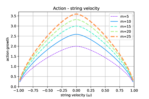
Figure 2: $a=\alpha=0$ and different masses

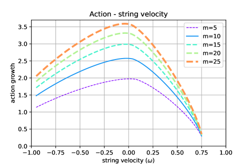
Figure 3: $a=0.2,\alpha=0$, different messes

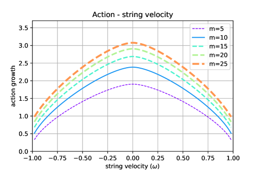
Figure 4: $a=0,\alpha=0.2$, different messes

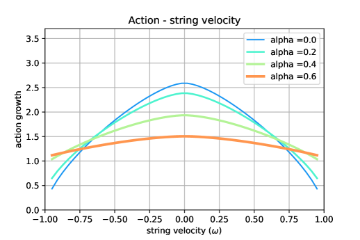
Figure 5: $m=10,a=0$, different acceleration

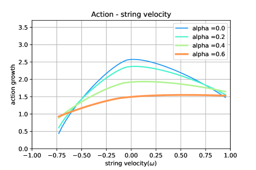
Figure 6: $m=10,a=-0.3$, different acceleration

4 Extremum point of the distribution

Since the integral region $r_{\pm}$ is independent of the value $\omega$, the partial derivative is

$$\frac{\partial}{\partial\omega}\Big{(}T_{\mathrm{str}}^{-1}\frac{dS_{\mathrm{NG}}}{dt}(\omega)\Big{)}=\frac{1}{2}\int_{r_{-}}^{r_{-}}d\sigma L^{-1/2}\frac{\partial L}{\partial\omega}.$$ (23)

Then in order to find the extremum point we have to find the point where $\displaystyle\frac{\partial L}{\partial\omega}=0$ is satisfied.

By fractorized form

We would like to find the above point by the method of Lagrange multipliers. We use the variables $x\coloneqq\omega$, $y\coloneqq\sigma_{0}$.

$$L(x,y)\coloneqq(1-ax)^{2}+xs_{1}(y)\frac{2a(1-ax)-x(y^{2}+\sigma^{2})}{f_{1}+f_{2}s_{1}(y)+f_{3}s_{2}(y)+f_{4}s_{3}(y)},$$ (24)

where $f_{n}$ are constant (independent of $\sigma$) determined by the properties of black holes (mass, angular momentum and acceleration) and $s_{n}$ are functions of $y$,

$$s_{n}(y)=\sum_{k=0}^{n}\sigma^{n-k}y^{k}.$$ (25)

We would like to find the maximal point with the constraint

$$\tilde{F}(x,y)\coloneqq F(y)(1-ax)^{2}-(a-(y^{2}+a^{2})x)^{2}=0.$$ (26)

We define the function

$$\tilde{L}(x,y,\lambda)\coloneqq L(x,y)+\lambda\tilde{F}(x,y)$$ (27)

and would like to find the extremum of this function.

Example 2 (Schwarzchild case).

For $a=0$ and $\alpha=0$, the problem is simplified as

$$L(x,y,\lambda)=1-x^{2}s_{1}\frac{y^{2}+\sigma^{2}}{f_{1}+s_{1}+s_{3}},\quad\tilde{F}(x,y)=F_{\mathrm{sch}}(y)-y^{3}x^{2}=0,\quad F_{\mathrm{sch}}(y)=y^{3}+y-2m.$$ (28)

The differentials are

$$\frac{\partial\tilde{L}}{\partial x} =-2x\Big{(}s_{1}\frac{(y^{2}+\sigma^{2})}{s_{3}+s_{1}-2m}+\lambda y^{3}\Big{)},$$ (29)

$$\frac{\partial\tilde{L}}{\partial y} =-x^{2}\frac{(s_{1}^{\prime}(y^{2}+\sigma^{2})+2ys_{1})(s_{3}+s_{1}-2m)-s_{1}(y^{2}+\sigma^{2})(s_{3}^{\prime}+s_{1}^{\prime})}{(s_{3}+s_{1}-2m)^{2}}+\lambda(3(1-x^{2})y^{2}+1),$$ (30)

$$\frac{\partial\tilde{L}}{\partial\lambda} =(1-x^{2})y^{3}+y-2m.$$ (31)

Then $x=\lambda=0$ is a solution and the last equation has the unique positive solution for $y$ when $x=0$. It is the same value to the horizon. ∎

In general,

$$\tilde{L}(x,y,\lambda) =(1-ax)^{2}+xs_{1}\frac{2a(1-ax)-x(y^{2}+\sigma^{2})}{f_{1}+f_{2}s_{1}+f_{3}s_{2}+f_{4}s_{3}}+\lambda\Big{(}(a-(y^{2}+a^{2})x)^{2}-(1-ax)^{2}\sum_{n=0}^{4}f_{n}y^{n}\Big{)}.$$ (32)

The derivatives are

$$\frac{\partial\tilde{L}}{\partial x} =-2a(1-ax)+s_{1}\frac{2a(1-2ax)-2x(y^{2}+\sigma^{2})}{f_{1}+f_{2}s_{1}+f_{3}s_{2}+f_{4}s_{3}}+2\lambda\Big{(}-(y^{2}+a^{2})(a-(y^{2}+a^{2})x)+a(1-ax)\sum_{n=0}^{4}f_{n}y^{n}\Big{)},$$

$$\frac{\partial\tilde{L}}{\partial y} =x\frac{s_{1}^{\prime}(2a(1-ax)-x(y^{2}+\sigma^{2}))-2xys_{1}}{f_{1}+f_{2}s_{1}+f_{3}s_{2}+f_{4}s_{3}}-xs_{1}(2a(1-ax)-x(y^{2}+\sigma^{2}))\frac{\sum_{n=0}^{4}f_{n+1}s_{n}^{\prime}}{(\sum_{n=0}^{4}f_{n+1}s_{n})^{2}}$$

$$\hskip 227.62204pt+\lambda\Big{(}-4xy(a-(y^{2}+a^{2})x)-(1-ax)\sum_{n=1}^{4}nf_{n}y^{n-1}\Big{)},$$

$$\frac{\partial\tilde{L}}{\partial\lambda} =-[(1-ax)^{2}(f_{0}-a^{2})+(1-ax)^{2}f_{1}y+(f_{2}+2ax)(1-ax)y^{2}+(1-ax)^{2}f_{3}y^{3}+((1-ax)^{2}f_{4}-x^{2})y^{4}].$$ (33)

We would like to confirm that the maximal point is independent of $\alpha$.

$$\frac{\partial\tilde{L}}{\partial x} =-2xs_{1}\frac{(y^{2}+\sigma^{2})}{f_{1}+s_{1}+f_{3}s_{2}+f_{4}s_{3}}+2\lambda y^{4}x,$$ (34)

$$\frac{\partial\tilde{L}}{\partial y} =x\frac{s_{1}^{\prime}(-x(y^{2}+\sigma^{2}))-2xys_{1}}{f_{1}+s_{1}+f_{3}s_{2}+f_{4}s_{3}}-xs_{1}(-x(y^{2}+\sigma^{2}))\frac{\sum_{n=0}^{4}f_{n+1}s_{n}^{\prime}}{(\sum_{n=0}^{4}f_{n+1}s_{n})^{2}}+\lambda\Big{(}4x^{2}y^{3}-\sum_{n=1}^{4}nf_{n}y^{n-1}\Big{)},$$ (35)

$$\frac{\partial\tilde{L}}{\partial\lambda} =x^{2}y^{4}-\sum_{n=0}^{4}f_{n}y^{n}.$$ (36)

The first and the second equations have solution $x=\lambda=0$. In this case, the third equation gives $y$ equal to the horizon value. We conclude that for non-rotating black holes $a=0$ the acceleration does not effect the maximal point.

5 Discussion

In this work we studied the effects of the probe string on the accelerating black hole spacetime, especially it has the angular momentum. We summarize the main results. The basic behavior of holographic complexity on the probe string is studied in [51]:

1. The effect of the string on the growth of complexity is minimized when the probe string is stationary.

The new properties we found are:

1. Effect of the angular momentum
   The rotation of the black hole causes the asymmetric behavior in the direction of string motion. In the past work [52] we only know that the black hole angular momentum causes the shift of the distribution between the growth of the action and the string motion. Now, in addition to this, we found the maximal value is independent of the black hole angular momentum (Fig.3 and Fig.3) by the numerical methods. Further, it will shed light on the relation between the rotation and the black hole acceleration as stated below.

2. Effect of the acceleration
   The acceleration of the black hole makes the string effect smaller. We also studied the relation between the effect of the black hole angular momentum and that of the acceleration by the analytic method. We found that when the black hole does not have the angular momentum the acceleration $\alpha$ does not change the maximal point (with respect to the string motion $\omega$). This result can also be checked visually by comparing Fig.3 ($a\neq 0$) and Figs.5, 5 ($a=0$).

In addition to these, we studied the maximal of the Nambu-Goto action in analytic way. We confirmed this results found in [51] analytically and confirmed that Property (0) is surely satisfied. We also found that the accelerating decreases the effect of the probe string while it does not shift the maximal point. This result is also confirmed numerically in Fig.5.

Acknnowledgments

This research is supported by Department of Physics, Toho University.

References

- [1] S. Chen and Y. Pei, “Holographic Complexity in AdS Accelerating Black Holes,” Int. J. Theor. Phys. 60 no. 3, (2021) 917–923.
- [2] K. Nagasaki, “Probe strings on AdS accelerating black holes,” arXiv:2108.05429 [hep-th].
- [3] Y. Sekino and L. Susskind, “Fast Scramblers,” JHEP 10 (2008) 065, arXiv:0808.2096 [hep-th].
- [4] L. Susskind, “Entanglement is not enough,” Fortsch. Phys. 64 (2016) 49–71, arXiv:1411.0690 [hep-th].
- [5] T. J. Osborne, “Hamiltonian complexity,” Reports on Progress in Physics 75 no. 2, 022001.
- [6] J. Watrous, “Quantum Computational Complexity,” ArXiv e-prints (Apr., 2008) , arXiv:0804.3401 [quant-ph].
- [7] S. Arora and B. Barak, “Computational Complexity: A Modern Approach”. Cambridge University Press, New York, NY, USA, 1st ed., 2009.
- [8] C. Moore and S. Mertens, “The Nature of Computation”. Oxford University Press, Inc., New York, NY, USA, 2011.
- [9] L. Susskind, “Computational Complexity and Black Hole Horizons,” Fortsch. Phys. 64 (2016) 24–43, arXiv:1403.5695 [hep-th].
- [10] P. Caputa, N. Kundu, M. Miyaji, T. Takayanagi, and K. Watanabe, “Liouville Action as Path-Integral Complexity: From Continuous Tensor Networks to AdS/CFT,” JHEP 11 (2017) 097, arXiv:1706.07056 [hep-th].
- [11] K. Hashimoto, N. Iizuka, and S. Sugishita, “Thoughts on Holographic Complexity and its Basis-dependence,” Phys. Rev. D98 no. 4, (2018) 046002, arXiv:1805.04226 [hep-th].
- [12] L. Susskind, “Black Holes and Complexity Classes,” arXiv:1802.02175 [hep-th].
- [13] L. Susskind, “Three Lectures on Complexity and Black Holes,” 2018. arXiv:1810.11563 [hep-th].
- [14] A. Bhattacharyya, P. Caputa, S. R. Das, N. Kundu, M. Miyaji, and T. Takayanagi, “Path-Integral Complexity for Perturbed CFTs,” arXiv:1804.01999 [hep-th].
- [15] S. Chapman and G. Policastro, “Quantum computational complexity from quantum information to black holes and back,” Eur. Phys. J. C 82 no. 2, (2022) 128, arXiv:2110.14672 [hep-th].
- [16] A. R. Brown and L. Susskind, “Second law of quantum complexity,” Phys. Rev. D97 no. 8, (2018) 086015, arXiv:1701.01107 [hep-th].
- [17] D. Carmi, S. Chapman, H. Marrochio, R. C. Myers, and S. Sugishita, “On the Time Dependence of Holographic Complexity,” JHEP 11 (2017) 188, arXiv:1709.10184 [hep-th].
- [18] Z.-Y. Fan and M. Guo, “Holographic complexity and thermodynamics of AdS black holes,” Phys. Rev. D100 (2019) 026016, arXiv:1903.04127 [hep-th].
- [19] A. Bernamonti, F. Galli, J. Hernandez, R. C. Myers, S.-M. Ruan, and J. Simon, “First Law of Holographic Complexity,” Phys. Rev. Lett. 123 no. 8, (2019) 081601, arXiv:1903.04511 [hep-th].
- [20] M. A. Nielsen, “A geometric approach to quantum circuit lower bounds,” eprint arXiv:quant-ph/0502070 (Feb., 2005) , quant-ph/0502070.
- [21] M. A. Nielsen, M. R. Dowling, M. Gu, and A. C. Doherty, “Quantum Computation as Geometry,” Science 311 (Feb., 2006) 1133–1135, quant-ph/0603161.
- [22] M. R. Dowling and M. A. Nielsen, “The geometry of quantum computation,” eprint arXiv:quant-ph/0701004 (Dec., 2007) , quant-ph/0701004.
- [23] J. M. Maldacena, “The Large N limit of superconformal field theories and supergravity,” Int. J. Theor. Phys. 38 (1999) 1113–1133, arXiv:hep-th/9711200 [hep-th]. [Adv. Theor. Math. Phys.2,231(1998)].
- [24] A. R. Brown, D. A. Roberts, L. Susskind, B. Swingle, and Y. Zhao, “Holographic Complexity Equals Bulk Action?,” Phys. Rev. Lett. 116 no. 19, (2016) 191301, arXiv:1509.07876 [hep-th].
- [25] A. R. Brown, D. A. Roberts, L. Susskind, B. Swingle, and Y. Zhao, “Complexity, action, and black holes,” Phys. Rev. D93 no. 8, (2016) 086006, arXiv:1512.04993 [hep-th].
- [26] M. Alishahiha, “Holographic Complexity,” Phys. Rev. D92 no. 12, (2015) 126009, arXiv:1509.06614 [hep-th].
- [27] S. Chapman, H. Marrochio, and R. C. Myers, “Complexity of Formation in Holography,” JHEP 01 (2017) 062, arXiv:1610.08063 [hep-th].
- [28] J. Tao, P. Wang, and H. Yang, “Testing holographic conjectures of complexity with Born-Infeld black holes,” Eur. Phys. J. C77 no. 12, (2017) 817, arXiv:1703.06297 [hep-th].
- [29] J. Jiang and X.-W. Li, “Modified ”complexity equals action” conjecture,” Phys. Rev. D100 no. 6, (2019) 066026, arXiv:1903.05476 [hep-th].
- [30] J. Jiang and B.-X. Ge, “Investigating two counting methods of the holographic complexity,” Phys. Rev. D99 no. 12, (2019) 126006, arXiv:1905.08447 [hep-th].
- [31] S. S. Gubser, “Drag force in AdS/CFT,” Phys. Rev. D74 (2006) 126005, arXiv:hep-th/0605182 [hep-th].
- [32] A. Nata Atmaja and K. Schalm, “Anisotropic Drag Force from 4D Kerr-AdS Black Holes,” JHEP 04 (2011) 070, arXiv:1012.3800 [hep-th].
- [33] D. S. Ageev and I. Y. Arefeva, “Holography and nonlocal operators for the BTZ black hole with nonzero angular momentum,” Theor. Math. Phys. 180 (2014) 881–893, arXiv:1402.6937 [hep-th]. [Teor. Mat. Fiz.180,no.2,147(2014)].
- [34] M. Moosa, “Evolution of Complexity Following a Global Quench,” JHEP 03 (2018) 031, arXiv:1711.02668 [hep-th].
- [35] Z. Fu, A. Maloney, D. Marolf, H. Maxfield, and Z. Wang, “Holographic complexity is nonlocal,” JHEP 02 (2018) 072, arXiv:1801.01137 [hep-th].
- [36] T. Numasawa, “Holographic Complexity for disentangled states,” arXiv:1811.03597 [hep-th].
- [37] D. Ageev, I. Aref ’eva, A. Bagrov, and M. I. Katsnelson, “Holographic local quench and effective complexity,” arXiv:1803.11162 [hep-th].
- [38] J. B. Griffiths, P. Krtous, and J. Podolsky, “Interpreting the C-metric,” Class. Quant. Grav. 23 (2006) 6745–6766, arXiv:gr-qc/0609056.
- [39] J. Podolsky, “Accelerating black holes in anti-de Sitter universe,” Czech. J. Phys. 52 (2002) 1–10, arXiv:gr-qc/0202033.
- [40] M. Appels, R. Gregory, and D. Kubiznak, “Thermodynamics of Accelerating Black Holes,” Phys. Rev. Lett. 117 no. 13, (2016) 131303, arXiv:1604.08812 [hep-th].
- [41] R. Gregory, “Accelerating Black Holes,” J. Phys. Conf. Ser. 942 no. 1, (2017) 012002, arXiv:1712.04992 [hep-th].
- [42] A. Anabalón, F. Gray, R. Gregory, D. Kubizňák, and R. B. Mann, “Thermodynamics of Charged, Rotating, and Accelerating Black Holes,” JHEP 04 (2019) 096, arXiv:1811.04936 [hep-th].
- [43] M. Appels, Thermodynamics of Accelerating Black Holes. PhD thesis, Durham U., Dept. of Math., 2018.
- [44] R. Gregory and A. Scoins, “Accelerating Black Hole Chemistry,” Phys. Lett. B 796 (2019) 191–195, arXiv:1904.09660 [hep-th].
- [45] M. Zhang and R. B. Mann, “Charged accelerating black hole in gravity,” Phys. Rev. D 100 no. 8, (2019) 084061, arXiv:1908.05118 [hep-th].
- [46] A. Ball and N. Miller, “Accelerating black hole thermodynamics with boost time,” Class. Quant. Grav. 38 no. 14, (2021) 145031, arXiv:2008.03682 [hep-th].
- [47] F. L. Carneiro, S. C. Ulhoa, and J. W. Maluf, “On the Black Hole Acceleration in the C-metric Space-time,” arXiv:2107.09806 [gr-qc].
- [48] H. Xu, “Minimal surfaces in AdS C-metric,” Phys. Lett. B 773 (2017) 639–643, arXiv:1708.01433 [hep-th].
- [49] M. J. Graham, K. E. S. Ford, B. McKernan, N. P. Ross, D. Stern, K. Burdge, M. Coughlin, S. G. Djorgovski, A. J. Drake, D. Duev, M. Kasliwal, A. A. Mahabal, S. van Velzen, J. Belecki, E. C. Bellm, R. Burruss, S. B. Cenko, V. Cunningham, G. Helou, S. R. Kulkarni, F. J. Masci, T. Prince, D. Reiley, H. Rodriguez, B. Rusholme, R. M. Smith, and M. T. Soumagnac, “Candidate electromagnetic counterpart to the binary black hole merger gravitational-wave event s190521g,” Phys. Rev. Lett. 124 (Jun, 2020) 251102. https://link.aps.org/doi/10.1103/PhysRevLett.124.251102.
- [50] H. Kodama, “Accelerating a Black Hole in Higher Dimensions,” Prog. Theor. Phys. 120 (2008) 371–411, arXiv:0804.3839 [hep-th].
- [51] K. Nagasaki, “Complexity of AdS5 black holes with a rotating string,” Phys. Rev. D96 no. 12, (2017) 126018, arXiv:1707.08376 [hep-th].
- [52] K. Nagasaki, “Complexity growth of rotating black holes with a probe string,” Phys. Rev. D98 no. 12, (2018) 126014, arXiv:1807.01088 [hep-th].