Single-photon scattering on a qubit. Space-time structure of the scattered field
Abstract
We study the space-time structure of the scattered field induced by the scattering of a narrow single-photon Gaussian pulse on a qubit embedded in 1D open waveguide. For a weak excitation power we obtain explicit analytical expressions for space and time dependence of reflected and transmitted fields which are, in general, are different from plain travelling waves. The scattered field consists of two parts: a damping part which represent a spontaneous decay of the excited qubit and a coherent, lossless part. We show that for large distance from qubit and at times long after the scattering event our theory provides the result which is well known from the stationary photon transport. However, the approach to the stationary limit is very slow. The scattered field decreases as the inverse powers of and as both the distance from the qubit and the time after the interaction increase.
pacs:
84.40.Az, 84.40.Dc, 85.25.Hv, 42.50.Dv, 42.50.PqI Introduction
Manipulating the propagation of photons in a one-dimensional waveguide coupled to an array of two-level atoms (qubits) may have important applications in quantum devices and quantum information technologies Rai2001 ; Roy2017 ; Gu2017 .
A single photon scattered by a single atom embedded in a 1D open waveguide was first considered in Shen2005a ; Shen2005b , where the authors employed the real 1D space description of the Dicke Hamiltonian and the Bethe-ansatz approach Rup1984 to derive the stationary solution for the photon transport. It was found that a photon with a frequency equal to that of the two-level atom can be completely reflected due to quantum interference. This property has been experimentally confirmed in the scattering of a microwave photon by a superconducting qubit Asta2010 ; Hoi2011 ; Hoi2013 .
Since then, theoretical calculations of the stationary photon transport in a 1D open waveguide with the atoms placed inside have been performed in a configuration space Shen2009 ; Cheng2017 ; Fang2014 ; Zheng2013 or by alternative methods such as those based on Lippmann-Schwinger scattering theory Roy2011 ; Huang2013 ; Diaz2015 , the input-output formalism Fan2010 ; Lal2013 ; Kii2019 , the non-Hermitian Hamiltonian Green2015 , and the matrix methods Green2021 ; Tsoi2008 .
Even though the stationary theory of the photon transport provides a useful guide to what one would expect in real experiment, it does not allow for a description of the dynamics of a qubit excitation and the evolution of a single-photon pulse.
Within the framework of the stationary scattering theories there are only incident and reflected plane waves in front of the qubit, and the transmitted plane wave behind the qubit. The reflected and transmitted amplitudes should be understood as the limits of time-dependent description when both the time after the scattering event and the distance from the qubit tend to infinity. Within this approach, all information about the temporal and spatial evolution of the field scattered by the qubit is completely lost. To obtain this information, it is necessary to consider a time-dependent problem, when the incident wave is a wave packet that depends on time and coordinates.
In practice, the qubits are excited by the photon pulses with finite duration and finite bandwidth. Therefore, to study the real time evolution of the photon transport and atomic excitation the time-dependent dynamical theories were developed Chen2011 ; Liao2015 ; Liao2016a ; Liao2016b ; Zhou2022 . In these works, the dynamics of the amplitudes of the qubit, transmitted, and reflected waves were considered with an incident single-photon Gaussian packet being scattered by the qubit. The main attention was paid to the reflected and transmitted spectra as the time after the scattering event tends to infinity. In this case, the field scattered by the qubit become plain waves and asymptotically approaches the stationary results for the photon transport.
Even though the time-dependent theory allows, in principle, to study the real-time evolution of the scattered field, the systematic and exhaustive discussion of this issue is absent except for several numerical plots Chen2011 ; Liao2015 ; Drob2000 . The investigation of the electric field induced by the propagation of a single-photon wave packet through a single atom embedded in a 1D waveguide has been performed in Dom2002 . However, in this paper the frequency dependence of transmitted and reflected fields has not been studied. The main attention was paid to the on-resonance dependance of transmittance and reflectance on the pulse width.
In the real case, the measurements are being performed shortly after the qubit excitation. Under these conditions the reflected and transmitted fields are not plain waves. Therefore, from the point of device applications, it is very important to study a real-time evolution and space structure of the scattered field.
In the present paper we consider the scattering of a narrow single-photon Gaussian pulse by a two-level artificial atom (qubit) embedded in an 1D open waveguide. We assume that the bandwidth of the pulse is much smaller than that of any other components of the system. It allows us to obtain the explicit analytical expressions for the scattered waveguide fields. The scattered fields consists of two parts: a damping part which represents a spontaneous decay of the excited qubit and a coherent, lossless part. We show that for large distance from qubit and at times long after the scattering event our theory for the reflected and transmitted amplitudes provides the result which is well known from the stationary scattering theories. However, in general, the structure of the scattered field is different from the stationary limit.
The paper is organized as follows. In Sec. II we introduce the basic parameters describing the transmitted and reflected amplitudes and their asymptotic properties. A general description of our model is given in Sec. III. The interaction between the qubit and electromagnetic field is described by Jaynes-Cummings Hamiltonian. The trial wave-function is taken within a single-excitation subspace. From time-dependent Schrodinger equation we obtain the single-photon amplitudes for forward and backward waves. The main result of the paper is given in Sec. IV. Here we construct the photon wavepacket for forward and backward propagating fields. We obtain the explicit expressions for the functions which are given in equations (3), (4). We show that as both a distance from the qubit and the time after scattering tend to infinity, the stationary results (1), (2) are recovered. The details of the calculations are given in Appendices A and B. The influence of the probing power, decoherence rate, and the non radiative losses on the transmitted and reflected fields are explained in Appendix C.
II Formulation of the problem
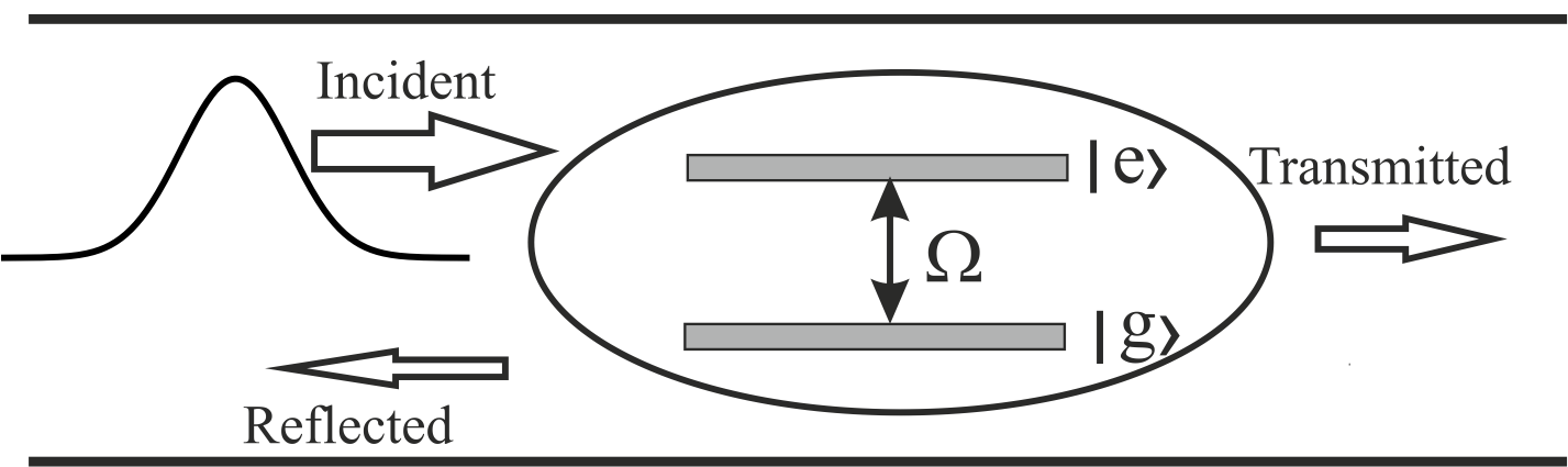
We consider the interaction of a single-photon Gaussian pulse with a two-level atom which is coupled to the waveguide modes with a strength . The excitation frequency of a qubit is (see Fig. 1). A qubit is considered as the point-like emitter which is placed in the point of the axis. We assume the interaction of incident pulse with the qubit starts at . It results in the reflected and transmitted fields whose space and time structure is the main subject of the paper.
Even though our treatment can be applied to a real two-level atom, we consider here an artificial two-level atom, a superconducting qubit operating at microwave frequencies. For subsequent calculations we take typical qubit’s parameters: the excitation frequency, GHz which corresponds to the wavelength cm, the rate of spontaneous emission into waveguide modes, MHz. We asssume the group velocity of electromagnetic waves is equal to that of a free space, m/s.
The analytical expressions for the transmission and reflection amplitudes found in a framework of stationary scattering approach for a monochromatic signal scattered by a two-level atom in an 1D open waveguide Shen2005a ; Shen2005b are as follows:
| (1) |
| (2) |
where is the photon frequency.
It follows from expression (1) that when the photon frequency coincides with the qubit frequency, then the value of T vanishes. In this case, the incident photon is completely reflected from the qubit. The reason for this perfect reflection is a coherent interference between the incident wave and the wave scattered by the qubit. It can be said that in this case, the qubit plays the role of an ideal mirror. This behavior was first observed experimentally in the scattering of a microwave photon by a superconducting qubit Asta2010 .
Strictly speaking the equations (1), (2) are valid if we assume a weak probing signal and neglect qubit’s pure dephasing, and non-radiative intrinsic losses, Hoi2013 . In our treatment below we assume the probe is weak. Under this assumption the pure dephasing and non-radiative losses can simply be incorporated in our treatment by adding the imaginary part to the qubit’s frequency , . We address this issue in a more detail in the Appendix C.
From general considerations, it is obvious that the plane wave solutions (1), (2) should be a limiting case of a time-dependent picture when both the distance from a qubit and the time after the scattering tend to infinity. Near the qubit, the scattered field is more complicated, the amplitude of which depends on the space-time coordinates x, t of the scattered field. In the general case, the transmission and reflection fields should have the following form:
| (3) |
| (4) |
The quantities that characterize the space-time structure of the scattered field must satisfy the following property: at . Their structure depends, of course, on the shape of the initial pulse. For a Gaussian wave packet, the structure of can be studied only by numerical methods Chen2011 ; Liao2015 .
In the present paper, we take the excitation pulse in the form of a Gaussian wave packet which is given by Liao2015 :
| (5) |
where is the length of a waveguide, is the wave vector corresponding to the center frequency of the pulse, and is the width in the k space. We note that the pulse (5) ensures that there is only a single photon in the wavepacket: .
For narrow pulse we obtain the explicit analytical expressions for the functions . These functions decrease relatively slow (as the inverse powers of x and t) for large both and , however, for and fixed , these functions do not tend to zero. It means that at relatively small distances from the qubit, the field is not uniform and the dependence of the transmission and reflection amplitudes on the frequency is more complicated than it follows from expressions (1), (2).
III The model
We consider a single qubit which is located at the point in an open linear waveguide. The Hilbert space of the qubit consists of the excited state , and the ground state . The Hamiltonian which accounts for the interaction between the qubit and electromagnetic field is as follows (we use units where throughout the paper):
| (6) |
where is Hamiltonian of bare qubit,
| (7) |
The photon operators , (), and , () describe forward and backward scattering waves, respectively; , are the rising and lowering spin operators, respectively: , . A spin operator . The quantity in (6) is the coupling between qubit and the photon field in a waveguide. We assume that the coupling is the same for forward and backward waves, .
Below we consider a single-excitation subspace with either a single photon being in a waveguide and the qubit being in the ground state, or there are no photons in a waveguide with the qubit being excited. Therefore, we limit Hilbert space to the following states:
| (8) |
A trial wave function in single-excitation subspace reads:
| (9) |
where is the amplitude of the qubit, , and are the single-photon amplitudes for forward and backward waves, respectively.
The equations for the quantities , , and can be found from time-dependent Schrodinger equation .
| (10) |
| (11) |
| (13) |
| (14) |
Substitution of (14) and (13) into equation (10) and application of Wigner-Weisskopf approximation provide the following expression for the qubit amplitude (the details of the derivation are given in Appendix A):
| (15) |
where
| (16) |
| (17) |
The form of insures the validity of a single-photon approximation: .
The integral in the righthand side of Eq.15 can be expressed in terms of the error function Grad2007 :
| (18) |
From now on we consider a narrow pulse where is a small quantity. In the leading order in we obtain from (18):
| (19) |
This approximation is valid for , .
Regarding the Eq. 19, it is worth noting that in our case a narrow Gaussian pulse can be approximated by a delta pulse with the amplitude :
| (20) |
Finally, the Eq.15 takes the form:
| (21) |
For initially unexcited qubit, , we obtain from (15) the following result for the qubit amplitude:
| (22) |
where
| (23) |
| (26) |
| (27) |
From (13) and (14) we may conclude that the amplitude of the forward propagating (transmitted) wave is equal to the amplitude of the backward propagating (reflected) wave, .
As is pointed in Sect.II and is proved in the Appendix C our treatment is valid if we consider a single-photon Gaussian pulse as a weak excitation probe. For single-photon transport the weak excitation means that the pulse duration is much longer than the spontaneous lifetime of the qubit, Fan2010 . In this case, the qubit is mostly in the ground state. Therefore, we can define the average number of probe photons per interaction time as , where is the power of the incident pulse Hoi2011 ; Hoi2013 . Taking MHz, GHz we can estimate the power of the incident single-photon Gaussian probe in a weak excitation limit, W. This value is within a reach of experimental technique Hoi2011 ; Hoi2013 .
IV Space-time structure of the scattered field
IV.1 Forward scattering field
The photon wave packet for forward propagating field behind the qubit is given by
| (28) |
where is given in (5).
In equations (28) and . The second condition insures the causality of propagating field which appears at the point behind the qubit not until the signal travels the distance after the scattering.
For forward scattering the summation over is replaced by the integration:
| (29) |
where we take a linear frequency dispersion well above the cutoff frequency of a waveguide.
The first sum in righthand side of (28) reads:
| (30) |
where we use a small approximation (19). Therefore, we may consider pre factor in (30) as the amplitude of incoming wave, .
For the second sum in righthand side of (28) we obtain:
| (31) |
where
| (32) |
| (33) |
The calculations of the quantities , are performed in the Appendix B. They are given by
| (34) |
| (35) |
where , is the exponential integral Abram1964 ; and are sine integral and cosine integral, respectively Grad2007 .
Combining (30) and (31) we obtain the forward propagating field behind the qubit in the following form:
| (37) |
where , .
It should be noted that the amplitude of transmitted field, in the first term in (37) is the result of a summation of the incident wave (30) with a part of the scattered field (2 in (35)). The second term in (37) is a damping part of the scattered field which represents a spontaneous decay of the excited qubit. The third term in (37) is a coherent, lossless part of the scattered field. As both a distance from the qubit and the time after the scattering tend to infinity these scattering fields die out leaving only the plane wave stationary solution.
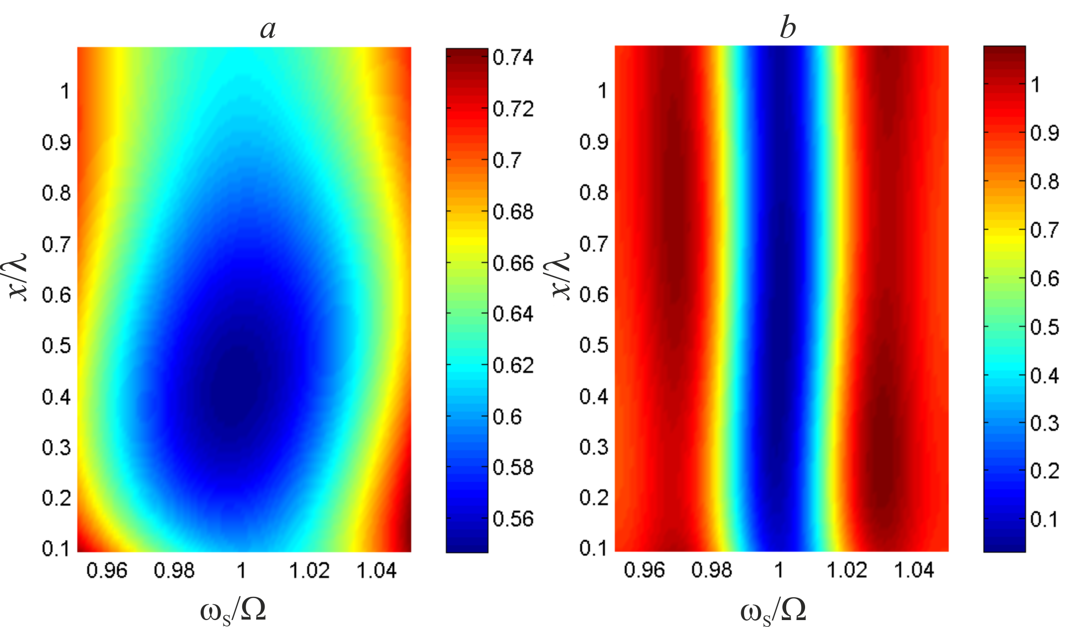
In Fig.2b we observe the off-resonance regions () where the transmittance is about larger than 1. This effect persists over wavelength scale. It can be attributed to the interference between incident wave and the field generating by the qubit itself. It does not contradict with the conception of the probability. In relation to our study the probability is inferred from the conservation of the energy flux: at any instant of time the input energy flux is the sum of the transmitted and reflected energy fluxes integrated over all space and over all frequencies. In our paper we calculate not the energy flux, but the electric field . Therefore, in this case the conception of the probability is not applicable. As aside comment it is worth noting that a similar amplification of the field exists in Fabry-Perot interferometer with semi-transparent mirrors Ley1987 .
IV.2 Backward scattering field
The photon wave packet for backward propagating field before the qubit is as follows:
| (38) |
where
| (39) |
| (40) |
In equations (38), (39), and (40) and . The second condition insures the causality of the backscattering field which appears at the point in front of the qubit not until the signal travels the distance after the scattering.
The quantities , can be calculated similar to the quantities , . The result is as follows:
| (41) |
| (42) |
where , .
Therefore, the backscattered field can be written in the following form:
| (43) |
where , . Here, as in the case of the forward scattering there are three terms in (43), stationary solution, damping, and coherent part of the scattered field.
The first terms in (37) and (43) are just the transmission and reflection amplitudes from the stationary theory. The second lines describe the field generated by spontaneous emission of excited qubit. This field dies out as the time tends to infinity. The third lines are the transmitted and reflected travelling waves which originate from the interaction of a qubit with the incident photon.
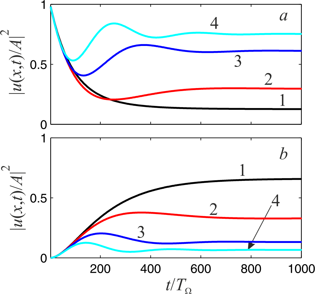
It is worth noting that the scattered fields (37) and (43) display oscillatory behavior in time as shown in Fig.4. These oscillations at the frequency originate from the interference between the first and the second (spontaneous decay) terms in expressions (37) and (43). To avoid the infinity of at we start the calculations in Fig.4 at mm distance from the qubit and at the time ps that insures the required condition .
There exists a deep analogy between time oscillations of our scattered fields and those of the decay probability in the dynamics of unstable quantum system Peshkin2014 . In both cases the time oscillations originate from the effective (after the averaging out the photon degrees of freedom) non-Hermitian Hamiltonian.
IV.3 The scattered field at large time
There are three time scales in our problem: , , and where . As was shown in (19) a weak excitation probe sets the upper bound on the time at which our theory is valid, . Therefore, we may safely satisfy the conditions , which are necessary to study the asymptotic of the transmitted (37) and reflected (43) fields for sufficiently large time.
If the time is sufficiently large and is fixed we may disregard the time dependent corrections in (37) and (43). In this case, we obtain from (37) the field behind the qubit:
From (44) we see that for the field at finite distance behind the qubit is non-zero. However, as tends to infinity () the last term in (44) disappears and we are left with the stationary transmission amplitude.
Similar calculations from (43) provides the field ahead of the qubit:
| (45) |
where is the reflection amplitude (2); , . For sufficiently large time the field at finite distance ahead of the qubit remains finite. However, as the tends to infinity () the last term in (45) disappears and we are left with the stationary reflection amplitude.
We investigate now how the scattered field (second terms in (44) and (45)) influences the amplitude-frequency curves (AFC) of transmitted and reflected signals. The dependence of AFCs on the distance from qubit is shown in Fig.5.
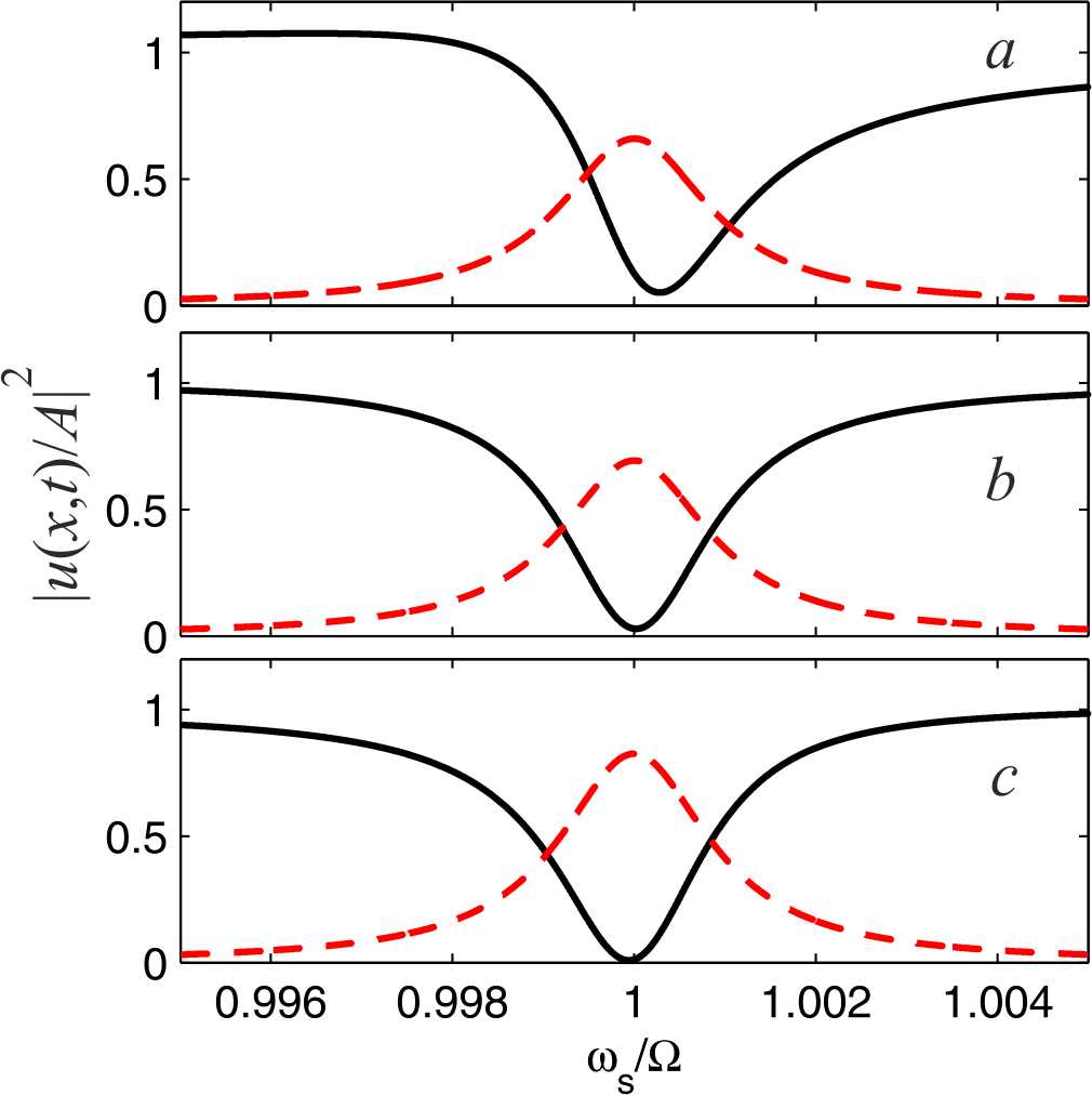
We see that a clear asymmetry is observed at mm () for transmitted AFC (Fig.5a). However, for larger the asymmetry persists as well. We see in Fig.5b and Fig.5c that the transmitted signal at resonance () is practically zero, while the amplitude of the reflected signal at resonance is appreciably smaller than unity. It can be attributed to the interference between two terms in (45)). In fact, from (45) we can write the squared modulus of the reflected field as where is the term in the round brackets in (45). The influence of on the reflected field at the 1 mm distance from the qubit is shown in Fig.6.
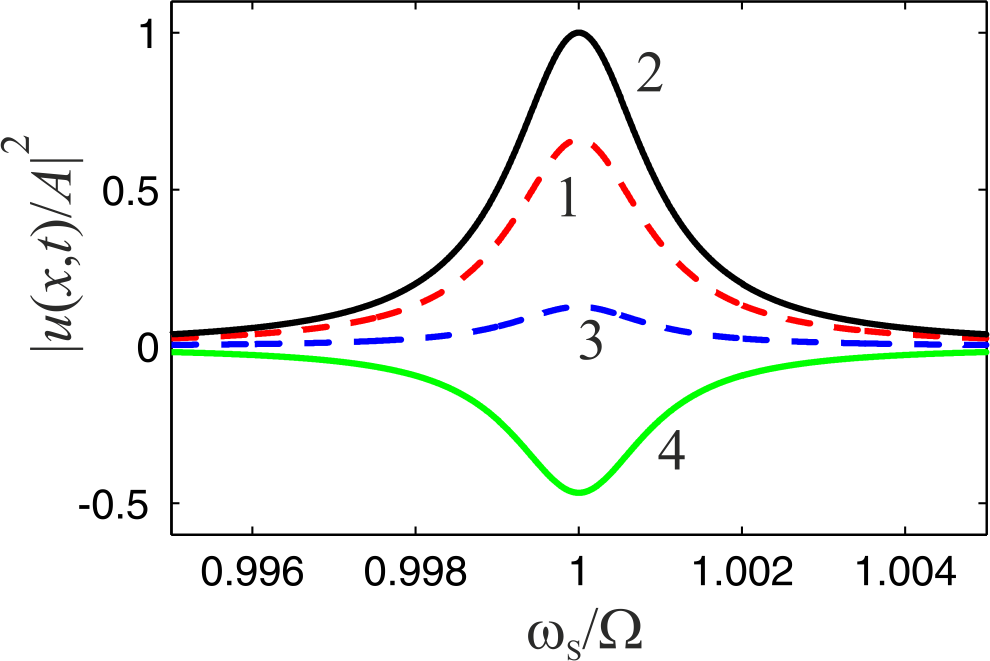
As is seen from this figure, the contribution of the interference term is negative (the curve 4 in Fig.6) and is significant. If the interference term in (45) is neglected we obtain for transmitted signal (curve 2 in Fig.6).
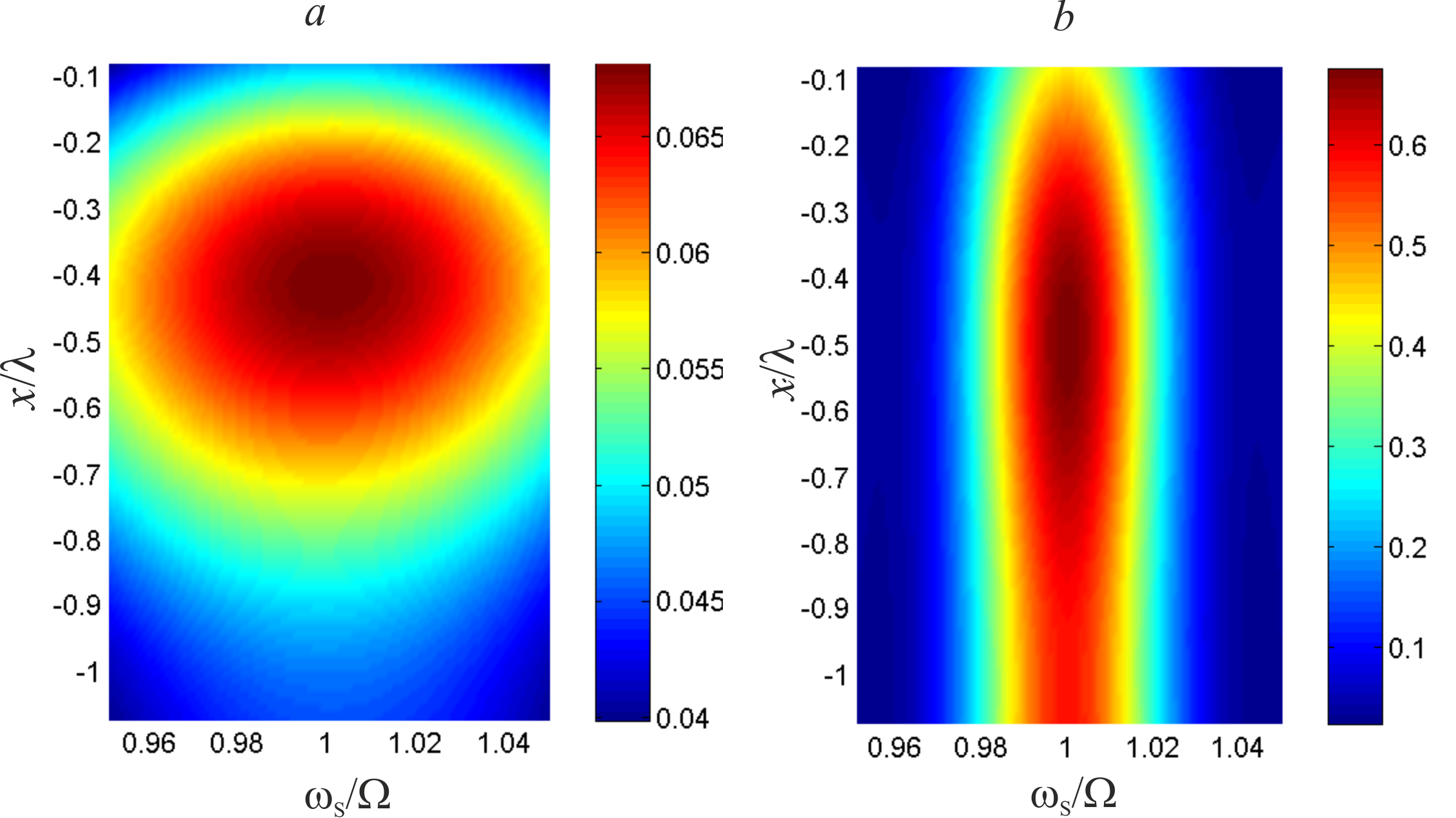
For off-resonant conditions, the interference effects persist both for reflected and transmitted fields. The influence of these effects on spatial dependence of the scattered fields is shown in Fig.7 for .
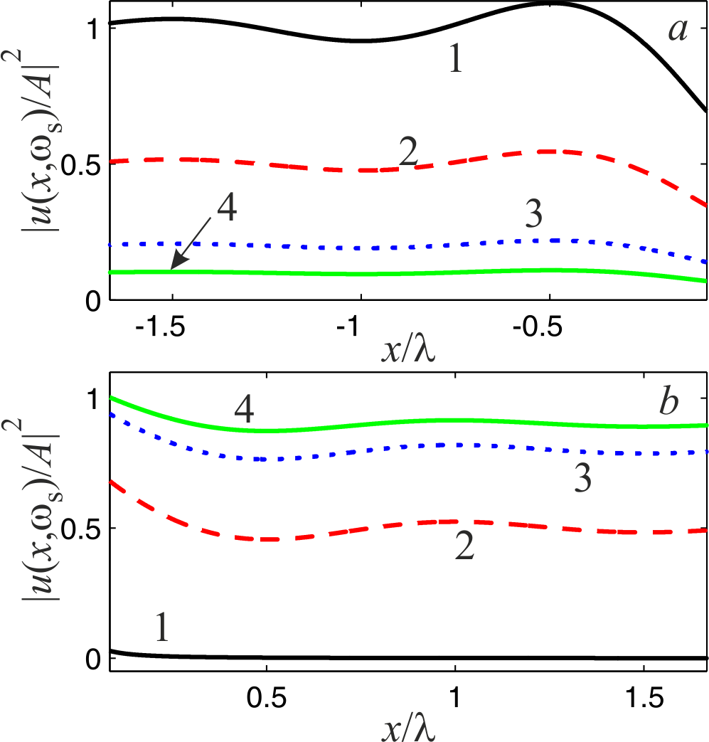
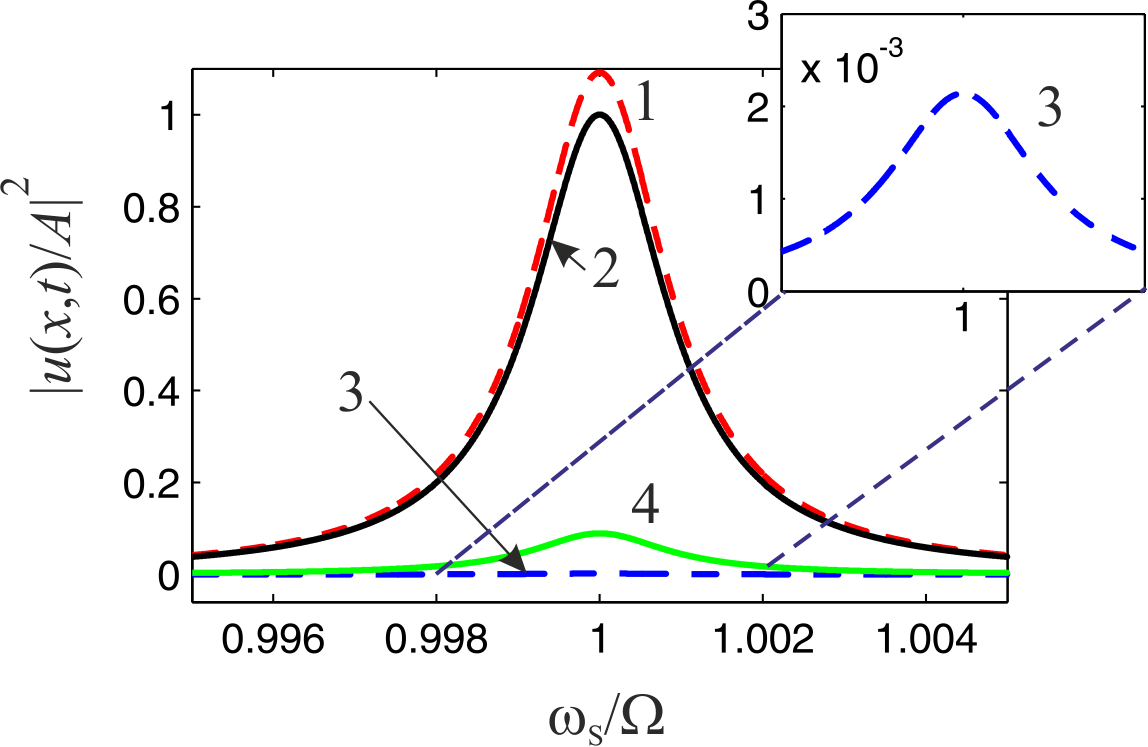
From Fig. 7a we see that the reflectance at is larger that 1 (see our comment below Fig.2b). This amplification can be explained by a constructive interference between incident and reflected waves as is shown in Fig.8. In this case the interference term (solid green line 4 in Fig.8) is positive (compare it with the line 4 in Fig.6) which gives rise to a small amplification of the reflected field in the resonance region.
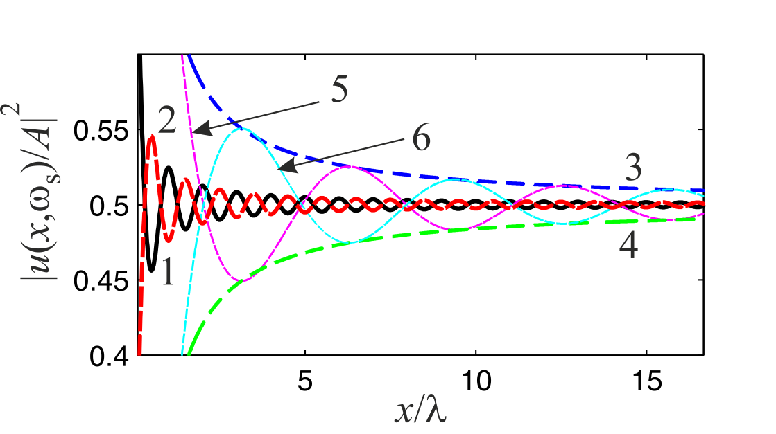
In principle, the interference effects can persist over relatively long distance. As an example we calculate from (44) and (45) the transmittance and reflectance for off-resonant frequency .
| (46) |
where , , .
| (47) |
where , , .
The behavior of these quantities at the distance comparable to the photon wavelength follows from the asymptotic of sine and cosine integrals for large arguments (48). The asymptotic behavior of interference effects calculated from (46) and (47) is shown in Fig.9. The envelopes (lines 3 and 4 in Fig.9) scale as .
IV.4 Asymptotic of the scattered field
The behavior of scattered fields at large and follows from the asymptotic of exponential integral function, sine integral, and cosine integral Grad2007 ; Jahnke .
| (48) |
where .
| (49) |
where .
With the aid of these approximations we obtain from (37) the asymptotic expression for forward scattering field.
| (50) |
where , , , , , .
The asymptotic expression for backward scattering field reads:
| (51) |
where , , , , , .
V Summary
In summary, we have developed the time-dependent theory of the scattering of a narrow single-photon Gaussian pulse on a qubit embedded in 1D open waveguide. For a weak power of incident pulse we have obtained explicit analytical expressions for the transmitted and reflected fields, their spatial and time dependence. We show that the scattered field consists of two parts: a damping part which represents a spontaneous decay of the excited qubit and a coherent, lossless part. The plain wave solution for transmission and reflection amplitudes which are well known from the stationary photon transport follow from our theory as the limiting case when both the distance from the qubit and the time after the scattering tend to infinity.
Even though our treatment can be applied to a real two-level atom, we consider in our paper an artificial two-level atom, a superconducting qubit operating at microwave frequencies at GHz range. For our calculations we take qubit frequency GHz which corresponds to wavelength cm. Our calculations show that spatial effects can persist on the scale of several ’s (see Fig. 9). For on-chip realization this length is not small compared with the dimensions of a superconducting qubit (typically several microns). The power of microwave signal is so low that the use of linear amplifiers for the detection of the qubit signal is a common practice. The current opportunity for on-chip realization of superconducting qubit with associated circuitry allows for the placement of the amplifier within the order of the wavelength from the qubit. Therefore, in microwave range the near-field effects can in principle be detectable.
We believe that the results obtained in this paper may have some practical applications in quantum information technologies including single-photon detection in a microwave domain as well as the optimization of the readout of a qubit’s quantum state.
Acknowledgements.
Ya. S. G. thanks V. Kurin who attracted the author’s attention to the problem considered in the present paper. The work is supported by the Ministry of Science and Higher Education of Russian Federation under the project FSUN-2020-0004.Appendix A Derivation of equation (15)
| (52) |
In accordance with Wigner-Weisskopf approximation the quantity under the integrals in (52) is assumed to be a slow function of time as compared to that of the exponents. Therefore, for times the integrand oscillates very rapidly and there is no significant contribution to the value of the integral. The most dominant contribution originates from times . We therefore evaluate at the actual time and move it out of the integrand. In this limit, the decay becomes a memoryless process (Markov process).
| (53) |
where
| (54) |
To evaluate this integral we extend the upper integration limit to infinity since there is no significant contribution for . Therefore, we obtain:
| (55) |
where represents the Cauchy principal value, which leads to a frequency shift. In what follows, we do not write explicitly this shift, which is assumed to be included in the qubit frequency.
Therefore, the equation (53) can be rewritten as follows:
| (56) |
where is the rate of spontaneous emission into waveguide modes, which is given by the Fermi golden rule:
| (57) |
For 1D case the summation over is replaced by the integration.
| (58) |
where we take a linear frequency dispersion well above the cutoff frequency of a waveguide.
Applying this prescription to (57) we express the coupling at the qubit resonance frequency () in terms of the rate of spontaneous emission :
| (59) |
The first term in right hand side of equation (56) then takes the form:
| (60) |
Appendix B Derivation of equations (34), (35)
B.1 Calculation of
The quantity in (32) consists of two terms: where
| (62) |
| (63) |
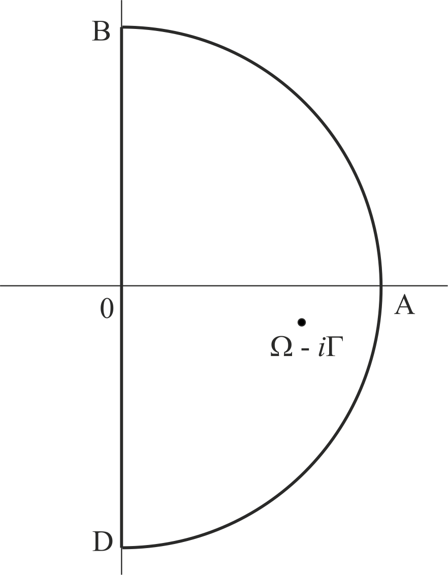
In the plane of complex the only pole lies in the lower part of the plane as shown in Fig.10. To calculate the last integral in (62) for we take a closed contour as shown in Fig.10. As there are no poles inside this contour we obtain:
| (64) |
| (65) |
The last integral in (65) can be expressed in terms of the exponential integral function (p.228, 5.1.4 in Abram1964 ):
| (66) |
where . Therefore, for we obtain
| (67) |
For the calculation of for we must take the contour in the lower part of the complex plane as shown in Fig.10:
| (68) |
From (68) we obtain
| (69) |
The last integral in (69) can be calculated similar to (66)
| (70) |
Therefore, for we obtain:
| (71) |
B.2 Calculation of
We rewrite (33) as follows:
| (73) |
In the integrand of (73) we introduce new variables , . We then obtain:
| (74) |
where .
For the first integral in (74) we obtain:
| (75) |
where we introduced the sine and cosine integrals:
| (76) |
Appendix C The influence of the probing power, decoherence rate, and the non radiative losses on the transmitted and reflected fields
With account for probing power and all losses the reflection coefficient can be expressed as Asta2010 ; Hoi2013
| (83) |
where , is the Rabi oscillation frequency, the square of which is proportional to the power, of incident wave, is the total decoherence rate where is pure dephasing and is the non-radiative intrinsic losses. The transmission coefficient can be found from the relation , which holds for a single emitter Asta2010 ; Hoi2013 .
| (84) |
| (86) |
The equations (85) and (86) coincide with (1) and (2) if we neglect pure dephasing and non-radiative losses. However, as it follows from (85) and (86) the pure dephasing and non-radiative losses can be included in the framework of our treatment simply by the redifinition of the qubit’s frequency , .
The coupling of the qubit to a waveguide can be described by a relevant quantity . If we disregard and we obtain the critical coupling which means at resonant frequency, a full extinction of transmitted signal, and a complete reflection . However, if we account for dephasing and non radiative losses the full extinction of transmitted field and complete reflection never happen.
References
- (1) J. M. Raimond, M. Brune, and S. Haroche, Manipulating quantum entanglement with atoms and photons in a cavity, Rev. Mod. Phys. 73, 565 (2001)., 565 (2001).
- (2) D. Roy, C. M. Wilson, and O. Firstenberg, Strongly interacting photons in one-dimensional continuum Rev. Mod. Phys. 89, 021001 (2017).
- (3) X. Gu, A. F. Kockum, A. Miranowicz, Y.-X. Liu, and F. Nori, Microwave photonics with superconducting quantum circuits, Phys. Rep. 718, 1 (2017).
- (4) J.-T. Shen and S. Fan, Coherent photon transport from spontaneous emission in one-dimensional waveguides, Optics Letters 30, 2001 (2005).
- (5) J. T. Shen and S. Fan, Coherent Single Photon Transport in a One-Dimensional Waveguide Coupled with superconducting Quantum Bits, Phys. Rev. Lett. 95, 213001 (2005).
- (6) V. I. Rupasov and V. I. Yudson, Rigorous theory of cooperative spontaneous emission of radiation from a lumped system of two-level atoms: Bethe ansatz method. Sov. Phys. JETP 60, 927 (1984).
- (7) O. Astafiev, A. M. Zagoskin, A. A. Abdumalikov, Yu. A. Pashkin, T. Yamamoto, K. Inomata, Y. Nakamura, and J. S. Tsai, Resonance Fluorescence of a Single Artificial Atom. Science 327, 840 (2010).
- (8) I.-C. Hoi, C. M. Wilson, G. Johansson, T. Palomaki, B. Peropadre, and P. Delsing, Demonstration of a Single-Photon Router in the Microwave Regime, Phys. Rev. Lett. 107, 073601 (2011).
- (9) I.-C. Hoi, C. M. Wilson, G. Johansson, J. Lindkvist, B. Peropadre, T. Palomaki, and P. Delsing, Microwave quantum optics with an artificial atom in one-dimensional open space, New Journal of Physics 15, 025011 (2013).
- (10) J.-T. Shen and S. Fan, Theory of single-photon transport in a single-mode waveguide. I. Coupling to a cavity containing a two-level atom. Phys. Rev. A 79, 023837 (2009).
- (11) M.-T. Cheng, J. Xu, and G. S. Agarwal, Waveguide transport mediated by strong coupling with atoms. Phys. Rev. A 95, 053807 (2017).
- (12) Y.-L. L. Fang, H. Zheng, and H. U. Baranger, One-dimensional waveguide coupled to multiple qubits photon-photon correlations. EPJ Quantum Technol. 1, 3 (2014).
- (13) H. Zheng and H. U. Baranger, Persistent Quantum Beats and Long-Distance Entanglement from Waveguide-Mediated Interactions. Phys. Rev. Lett. 110, 113601 (2013).
- (14) D. Roy, Correlated few-photon transport in one-dimensional waveguides: Linear and nonlinear dispersions, Phys. Rev. A 83, 043823 (2011).
- (15) J.-F. Huang, T. Shi, C. P. Sun, and F. Nori, Controlling single-photon transport in waveguides with finite cross section, Phys. Rev. A 88, 013836 (2013).
- (16) G. Diaz-Camacho, D. Porras, and J. J. Garcia-Ripoll, Photon-mediated qubit interactions in one-dimensional discrete and continuous models. Phys. Rev. A 91, 063828 (2015).
- (17) S. Fan, S. E. Kocabas, and J.-T. Shen, Input-output formalism for few-photon transport in one-dimensional nanophotonic waveguides coupled to a qubit, Phys. Rev. A 82, 063821 (2010).
- (18) K. Lalumiere, B. C. Sanders, A. F. van Loo, A. Fedorov, A. Wallraff, and A. Blais, Input-output theory for waveguide QED with an ensemble of inhomogeneous atoms. Phys. Rev. A 88 043806 (2013).
- (19) A. H. Kiilerich and K. Molmer, Input-Output Theory with Quantum Pulses. Phys. Rev. Lett. 123, 123604 (2019).
- (20) Ya. S. Greenberg and A. A. Shtygashev, Non hermitian Hamiltonian approach to the microwave transmission through a one-dimensional qubit chain. Phys.Rev. A 92, 063835 (2015).
- (21) Ya. S. Greenberg, A. A. Shtygashev, and A. G. Moiseev, Waveguide band-gap N-qubit array with a tunable transparency resonance. Phys.Rev. A 103, 023508 (2021).
- (22) T. S. Tsoi and C. K. Law, Quantum interference effects of a single photon interacting with an atomic chain. Phys. Rev. A 78, 063832 (2008).
- (23) Y. Chen, M. Wubs, J. Mork, and A. F. Koendrink, Coherent single-photon absorption by single emitters coupled to one-dimensional nanophotonic waveguides, New J. Phys. 13,103010 (2011).
- (24) Z. Liao, X.Zeng, S.-Y. Zhu, and M. S. Zubairy, Single-photon transport through an atomic chain coupled to a one-dimensional nanophotonic waveguide. Phys. Rev. A92, 023806 (2015).
- (25) Z. Liao, H. Nha, and M. S. Zubairy, Dynamical theory of single-photon transport in a one-dimensional waveguide coupled to identical and nonidentical emitters. Phys. Rev. A 94, 053842 (2016).
- (26) Z. Liao, X. Zeng, H. Nha, and M. S. Zubairy, Photon transport in a one-dimensional nanophotonic waveguide QED system Phys. Scr. 91, 063004 (2016).
- (27) C. Zhou, Z. Liao, and M. S. Zubairy, Decay of a single photon in a cavity with atomic mirrors. Phys. Rev. A 105, 033705 (2022).
- (28) G. Drobny, M. Havukainen, and V. Buzek, Stimulated emission via quantum interference Scattering of one-photon packets on an atom in a ground state. J. Mod. Optics 47, 851 (2000).
- (29) P. Domokos, P. Horak, and H. Ritsch, Quantum description of light-pulse scattering on a single atom in waveguides. Phys. Rev. A 65, 033832 (2002).
- (30) M. Ley, R. Loudon, Quantum theory of high resolution length measurement with a Fabry Perot interferometer. J. Mod. Opt. 34, 227 (1987).
- (31) M. Peshkin, A. Volya, and V. Zelevinsky, Non-exponential and oscillatory decays in quantum mechanics. Europ. Phys. Lett. 107, 40001 (2014).
- (32) M. Abramowitz and I. A. Stegun, Handbook of Mathematical Functions with Formulas, Graphs, and Mathematical Tables, NIST, 1964.
- (33) I. S. Gradshteyn and I. M. Ryzhik Table of Integrals, Series, and Products. Elsevier Inc. 7-th ed. Amsterdam 2007, 1220 pages.
- (34) E. Jahnke, F. Emde, F. Losch, Tables of higher functions. 1965, 7th ed.