A Heteroskedasticity-Robust Overidentifying Restriction Test with High-Dimensional Covariates

Abstract

We propose a new overidentifying restriction test for linear instrumental variable models. The novelty of the proposed test is that it allows the number of covariates and/or instruments to be larger than the sample size and is robust to heteroskedastic errors. We show that the test has the desired theoretical properties under sparse high-dimensional models and is more powerful than existing overidentification tests. First, we introduce a test based on the maximum norm of multiple parameters that could be high-dimensional. The theoretical power based on the maximum norm is shown to be higher than that in the modified Cragg-Donald test (Kolesár,, 2018), which is the only existing test allowing for large-dimensional covariates. Second, following the principle of power enhancement (Fan et al.,, 2015), we introduce the power-enhanced test, with an asymptotically zero component used to enhance the empirical power against some extreme alternatives with many locally invalid instruments. Focusing on hypothesis testing, we also provide a feasible estimator of endogenous effects for practitioners when instrument validity is not rejected. The simulation results show the superior performance of the proposed test, and the empirical power enhancement is clear. Finally, an empirical example of the trade and economic growth nexus demonstrates the usefulness of the proposed tests.

JEL classification: C12, C21, C26, C55
Keywords: overidentification test, maximum test, heteroskedasticity, power enhancement, data-rich environment.

1 Introduction

The instrumental variable (IV) approach is essential for the estimation and inference of endogenous treatment effects. Recently, the high-dimensional model has been the focal point of some IV-related studies, motivated by the increasing availability of large datasets, such as large survey data, clinical data, and administrative data. It is common to consider high-dimensional IV models where the number of covariates is vast, the number of potential IVs is enormous, or both. The consistency and asymptotic normality of IV estimation depend on the validity of the IVs. This paper concerns the overidentifying restriction test for IV validity in high dimensions, where the number of covariates and/or IVs could be even larger than the sample size.

The classic Sargan test (Sargan,, 1958) and J test (Hansen,, 1982) deal with a fixed number of IVs. Some recent overidentification tests consider a model with a large number of IVs. For example, Lee and Okui, (2012) proposed a modified Sargan test compatible with an increasing number of IVs under homoskedasticity. Chao et al., (2014) proposed an overidentification test robust to many IVs and heteroskedasticity following jackknife IV estimation (Angrist et al.,, 1999). Carrasco and Doukali, (2021) extended this method based on regularized jackknife IV estimation (Hansen and Kozbur,, 2014; Carrasco and Doukali,, 2017) to allow the number of IVs to be larger than the sample size.

All the tests mentioned above require the number of covariates in the structural equation to be fixed. A closely related earlier work is Kolesár, (2018), which extended Anatolyev and Gospodinov, (2011) and proposed a modified Cragg-Donald (MCD) test that allows a growing number of covariates. However, this test requires the total number of instruments ($p_{z}$) and covariates ($p_{x}$), $p=p_{z}+p_{x}$, to be less than the sample size $n$, and the test has poor empirical power when $p\approx n$. Within the context of overidentification tests, we refer to tests (including the MCD test and Chao et al., (2014)) that are based on a limiting $\chi^{2}$ distribution as “$\chi^{2}$-type tests”. None of the existing $\chi^{2}$-type tests allows $p>n$ with large $p_{x}$.

Recent works (Belloni et al.,, 2014; Chernozhukov et al.,, 2015; Guo et al., 2018a, ) have proposed estimation and inference methodologies for endogenous treatment effects under high dimensions with $p>n$. An overidentifying restriction test on IV validity is still unavailable for this scenario. This motivates our work. The proposed test allows the number of covariates $p_{x}$ and/or IVs $p_{z}$ to be greater than the sample size and is robust to heteroskedastic errors. It can check the validity of any overidentified subset of IVs and is scale invariant, making it a useful tool for empirical researchers. Although our paper focuses on the overidentification test, we suggest an endogenous treatment effect estimator when the null hypothesis is not rejected. Both the theoretical and numerical results support the suitability of this estimator.

1.1 Main Results and Contributions

First, we propose testing IV validity by designing a maximum test (M test) based on a maximum norm of multiple parameters that may be high dimensional. We call this test statistic the M statistic. Under some commonly imposed sparsity assumptions (Belloni et al.,, 2012, 2014), the M test has the correct asymptotic size; the M test has advantages for the setting of $p_{x}>n$, where existing $\chi^{2}$-type tests are not feasible. Moreover, the M test has better power than $\chi^{2}$-type tests under sparsity when $p$ grows with the sample size but $p<n$. Second, we propose an add-on asymptotically zero quadratic statistic (Q statistic) to improve the empirical power when the model includes many “locally invalid” IVs (meaning the alternatives have weak individual signals; for details, see Section 3.2) in finite samples. The resulting test, called the power-enhanced M test (PM test), rejects the null hypothesis when either the M or Q statistic is greater than the critical value of the significance level $\alpha$. Our paper extends the principle of power enhancement developed by Fan et al., (2015) and Kock and Preinerstorfer, (2019) to the popular IV model and overidentification test. The PM test always has noninferior theoretical power to the original M test by design. In simulations, we show that the empirical power of the PM test is indeed noninferior to that of the M test, and it is substantially improved when many IVs are locally invalid.

The PM test is an indispensable complement to the literature on postselection estimation and inference for endogenous treatment effects in high-dimensional settings (Belloni et al.,, 2012, 2014). These popular methodologies for sparse high-dimensional IV models are based on known IV validity. In practice, the IV validity is usually unknown. Our overidentification test is necessary for applications with many covariates and the IV set being either high- or low-dimensional.

We construct the tests using bias-corrected high-dimensional estimators. Specifically, the M test is implemented based on the maximum norm of the high-dimensional IV invalidity level estimator following the maximum test in a linear regression model (Chernozhukov et al.,, 2013; Zhang and Cheng,, 2017). The asymptotically zero Q statistic follows an inferential procedure for a quadratic form of high-dimensional parameters (Guo et al.,, 2019; Cai and Guo,, 2020; Guo et al.,, 2021). We extend the literature on quadratic form inference to the heteroskedasticity case.

In theory, we show that the M test has the correct asymptotic size with asymptotic power one when the maximum norm of the IV invalidity vector is of order $\sqrt{\log p_{z}/n}$. When $p_{z}$ is fixed, the M test can detect invalid IVs at a parametric rate, the same order of magnitude as the Sargan test in low dimensions. For sparse models with a growing $p_{z}$, the M test is shown to achieve higher asymptotic power than the existing $\chi^{2}$-type tests; the latter can only consistently detect the alternatives at the rate $p_{z}^{1/4}/\sqrt{n}$ (for details, see Section 3, Remark 9). Furthermore, the asymptotically zero Q statistic guarantees a higher asymptotic power of the PM test than the $\chi^{2}$-type tests when $p_{z}$ is proportional to $n$ (see Section 3, Remark 10). Computationally, the test can be easily implemented following the steps in Algorithm 1.

The simulation studies show that the M test has an apparent power improvement over the MCD test. For $p>n$ with large $p_{x}$, for which our proposal is the only feasible method, the M test shows satisfactory performance in terms of size and power. Under many locally invalid IVs, the PM test substantially improves the power compared to the original M test, with empirical type I error controlled at the nominal level.

In the empirical study, we revisit the effect of trade on economic growth. We perform different tests on an IV model with a large number of covariates. We consider an overidentified set of instruments, including several possibly invalid instruments, such as energy usage and business environment. The PM test strongly rejects the null hypothesis of the correct specification well under the 1% level. In contrast, the M test rejects the null hypothesis under 5%, and the MCD test fails to reject at the 5% level, indicating the superiority of the PM test under high-dimensional IV models.

We summarize the main contributions as follows:

1. We propose an overidentification test for IV models with high-dimensional data. To our knowledge, this is the first overidentification test for $p>n$ with large $p_{x}$. It is more powerful than existing $\chi^{2}$-type tests under certain sparsity restrictions when $p<n$.

2. Our test is robust to heteroskedasticity, which is essential in IV models. Our paper extends the current high-dimensional statistical literature on the maximum norm or quadratic form inference to heteroskedastic data.

3. We develop a power enhancement procedure in the context of an IV validity test. The asymptotically zero component improves empirical power against many local violations of the null hypothesis.

1.2 Other Related Literature

Often with the assumption of sparsity, $L_{1}$ regularized regression methods are commonly used to address high-dimensional problems with more covariates and IVs than the sample size (Belloni et al.,, 2012, 2014; Chernozhukov et al.,, 2015). A strand of literature has studied the estimation and inference of endogenous treatment effects without prior knowledge about IV validity (Kang et al.,, 2016; Guo et al., 2018a, ; Windmeijer et al.,, 2019, 2021; Sun et al.,, 2021; Ye et al.,, 2021; Fan and Wu,, 2022; Liang et al.,, 2022). Among these works, Guo et al., 2018a discussed inference for the treatment effect in the presence of possibly invalid IVs and high-dimensional covariates. However, these methods often require assumptions on the proportion of valid IVs, such as the majority rule Kang et al., (2016); Windmeijer et al., (2019). In addition, Guo, (2021) pointed out that the selection of valid IVs might suffer from selection error in finite samples. Our M test and its power-enhanced version work even if the majority rule is violated, and they show desirable finite sample performance based on our simulation and empirical results. Our test is also related to general signal detection works, including Donoho and Jin, (2004); Arias-Castro et al., (2011), and high-dimensional testing problems (Ingster and Suslina,, 2003). Our theoretical framework does not cover the examiner or judge designs (Arnold et al.,, 2022; Frandsen et al.,, 2023) with high-dimensional dummy IVs, which is a popular standalone application. This interesting case is left for future study. In addition, our methodology relates to the study of high-dimensional IV models from the perspective of estimation (Donald and Newey,, 2001; Okui,, 2011; Bai and Ng,, 2010; Carrasco,, 2012; Bekker and Crudu,, 2015; Fan and Zhong,, 2018; Zhu,, 2018). We also refer to Andrews et al., (2019) for a recent and comprehensive review of the weak IV literature.

Other literature (Liao,, 2013; Cheng and Liao,, 2015; Caner et al.,, 2018; Chang et al., 2021b, ) has studied moment condition selection under the GMM framework, requiring prior information about some moment conditions known to be valid. Chang et al., 2021a considered the overidentification test in high-dimensional settings using marginal empirical likelihood ratios and a selective subset of moment conditions. This paper also relates to a growing body of literature on quadratic form inference, such as Fan et al., (2021), with applications to the Markowitz mean-variance portfolio.

Finally, let us discuss the link between our paper and the inspiring power enhancement literature (Fan et al.,, 2015; Kock and Preinerstorfer,, 2019). For our overidentification test, the main task is primarily performed by the M test, although its empirical power can be further enhanced with a specific type of alternative (many local violations). There is a possibility of further improving the theoretical power of the overidentification test proposed by this paper. Nonetheless, additional efforts will be needed to fill the gap between the principle of power enhancement and the specific context of the overidentification test with high-dimensional covariates. Another point to consider is the choice of vector norm suggested by Kock and Preinerstorfer, (2021), who constructed an optimal high-dimensional test based on $L_{q}$ norm-based tests with $q\in(0,\infty]$ in a general framework. In light of Kock and Preinerstorfer, (2021), asymptotically unbiased estimators of $L_{q}$ norms are required to build a bridge from the theoretical power enhancement results to practical implementations with $p>n$. The theoretical properties of bias-corrected Lasso estimators for the maximum norm (Zhang and Cheng,, 2017) and squared $L_{2}$ norm (Cai and Guo,, 2020) are well known. However, this is not the case for the general $L_{q}$ norm. Due to these technical complications, and to focus on the central message of the current paper, we employ more easily implemented methodologies based on the maximum norm and $L_{2}$ norm for the $p>n$ case. More details are given in the last several paragraphs of Section 3.2.

Notation. We consider $p=p(n)$ as a function of $n$ and discuss the asymptotics where $n$ and $p$ jointly diverge to infinity. The phrase “with probability approaching one as $n\to\infty$” is abbreviated as “w.p.a.1”. An absolute constant is a positive, finite constant that is invariant with the sample size. We use “$\stackrel{{\scriptstyle p}}{{\longrightarrow}}$” and “$\stackrel{{\scriptstyle d}}{{\longrightarrow}}$” to denote convergence in probability and distribution, respectively. For any positive sequences $a_{n}$ and $b_{n}$, “$a_{n}\lesssim b_{n}$” means there exists some absolute constant $C$ such that $a_{n}\leq Cb_{n}$, “$a_{n}\gtrsim b_{n}$” means $b_{n}\lesssim a_{n}$, and “$a_{n}\asymp b_{n}$” indicates $a_{n}\lesssim b_{n}$ and $b_{n}\lesssim a_{n}$. Correspondingly, “$\lesssim_{p}$”, “$\gtrsim_{p}$” and “$\asymp_{p}$” indicate that the aforementioned relations “$\lesssim$”, “$\gtrsim$” and “$\asymp$” hold w.p.a.1. We use $[n]$ for some $n\in\mathbb{N}$ to denote the integer set $\{1,2,\cdots,n\}$. For a $p$-dimensional vector $x=(x_{1,}x_{2},\cdots,x_{p})^{\top}$, the number of nonzero entries is $\|x\|_{0}$, the $L_{2}$ norm is $\left\|x\right\|_{2}=\sqrt{\sum_{j=1}^{p}x_{j}^{2}}$, the $L_{1}$ norm is $\left\|x\right\|_{1}=\sum_{j=1}^{n}\left|x_{j}\right|$, and its maximum norm is $\|x\|_{\infty}=\max_{j\in[p]}|x_{j}|$. For a $p\times p$ matrix $A=(A_{ij})_{i,j\in[p]}$, we define the $L_{1}$ norm $\|A\|_{1}=\max_{j\in[p]}\sum_{i\in[p]}|A_{ij}|$ and the maximum norm $\|A\|_{\infty}=\max_{i,j\in[p]}|A_{i,j}|$. “$A\succ 0$” implies the positive definiteness of $A$. For any positive definite $A$ with spectral decomposition $U\Lambda U^{\top}$, we define $A^{1/2}=U\Lambda^{1/2}U^{\top}$ with $\Lambda^{1/2}$ being the diagonal matrix composed of the square roots of the corresponding diagonal elements of $\Lambda$. We use ${\rm diag}(A)$ to denote the diagonal matrix composed of the diagonal elements of $A$. We define ${\rm I}_{A}(x,y)=x^{\top}Ay$ and ${\rm Q}_{A}(x)={\rm I}_{A}(x,x)$ for any vectors $x,y\in\mathbb{R}^{p}$. We use $0_{p}$ to denote the $p\times 1$ null vector, $1_{p}$ to denote the $p\times 1$ all-one vector, and $I_{p}$ to denote the $p$-dimensional identity matrix. The indicator function is ${\textbf{1}}(\cdot)$. Finally, for any $a,b\in\mathbb{R}$, we use $a\vee b$ and $a\wedge b$ to denote $\max(a,b)$ and $\min(a,b)$, respectively.

The remainder of the paper is organized as follows. In Section 2, we introduce the model and a treatment effect estimator. Section 3 provides the M test and its power-enhanced version with their asymptotic properties. Section 4 demonstrates the finite sample performance of the PM test by Monte Carlo simulations. Section 5 provides an empirical example. Section 6 concludes the paper. Technical proofs and additional simulation results are given in the Appendix.

2 The Model and Endogenous Treatment Effect Estimation

We consider the following classic linear IV model: for $i=1,2,\dots,n$,

$$Y_{i} =D_{i}\beta+X_{i\cdot}^{\top}\varphi+Z_{i\cdot}^{\top}\pi+e_{i},\quad \mathbb{E}(e_{i}|Z_{i\cdot},X_{i\cdot})=0,$$ (1)

$$D_{i} =X_{i\cdot}^{\top}\psi+Z_{i\cdot}^{\top}\gamma+\varepsilon_{i2},\quad \mathbb{E}(\varepsilon_{i2}|Z_{i\cdot},X_{i\cdot})=0,$$

where $Y_{i}\in\mathbb{R}$ denotes the outcome variable, $D_{i}\in\mathbb{R}$ denotes the endogenous variable, and $X_{i\cdot}\in\mathbb{R}^{p_{x}}$ and $Z_{i\cdot}\in\mathbb{R}^{p_{z}}$ denote the covariates and the instrumental variables, respectively. We focus on the setting of a scalar endogenous variable $D_{i}$, which is common in the literature (Kolesár,, 2018; Windmeijer et al.,, 2019; Mikusheva and Sun,, 2020). The parameter of interest $\beta$ is interpreted as the treatment effect. $\varphi$, $\pi$, $\psi$, and $\gamma$ are coefficients of conformable dimensions in the model. $D_{i}$ is endogenous due to the correlation between $e_{i}$ and $\varepsilon_{i2}$, even conditional on all instruments and covariates. Our proposed overidentification test operates via a random sample $\{Y_{i},D_{i},X_{i\cdot},Z_{i\cdot}\}_{1\leq i\leq n}$. We denote $Y=(Y_{1},Y_{2},\cdots,Y_{n})^{\top}$, $D=(D_{1},D_{2},\cdots,D_{n})^{\top}$, $X=[X_{1\cdot},X_{2\cdot},\cdots,X_{n\cdot}]^{\top}$ and $Z=[Z_{1\cdot},Z_{2\cdot},\cdots,Z_{n\cdot}]^{\top}$.

We allow heteroskedastic errors in model (1) so that ${{\rm Var}}(e_{i}|Z_{i\cdot},X_{i\cdot})$ and ${{\rm Var}}(\varepsilon_{i2}|Z_{i\cdot},X_{i\cdot})$ may vary with $i$. As discussed in Section 1, the test allows $p=p_{x}+p_{z}\to\infty$ for any combination of $p_{x}$ and $p_{z}$. We also impose a sparsity assumption on model (1), following the literature on similar models with high-dimensional IVs and baseline covariates (e.g., Belloni et al.,, 2012, 2014; Kolesár et al.,, 2015; Guo et al., 2018b, ).

We consider the reduced form of model (1),

$$Y=X\Psi+Z\Gamma+\varepsilon_{1},$$ (2)

$$D=X\psi+Z\gamma+\varepsilon_{2},$$

where $\Psi=\psi\beta+\varphi$, $\Gamma=\gamma\beta+\pi$ and $\varepsilon_{1}=\varepsilon_{2}\beta+e$ with $e=(e_{1},e_{2},\cdots,e_{n})^{\top}$ and $\varepsilon_{2}=(\varepsilon_{12},\varepsilon_{22},\cdots,\varepsilon_{n2})^{\top}$. Following the literature on high-dimensional models, we impose the sparsity assumption on model (2). We define the sparsity index $s=\max\{\|\varphi\|_{0}+\|\pi\|_{0},\|\psi\|_{0}+\|\gamma\|_{0},\|\Psi\|_{0}+\|\Gamma\|_{0}\}$. For simplicity, we also use $s$ to regulate the sparsity of $\Psi$ and $\Gamma$, which can be induced by the sparsity of the coefficient vectors in model (1). We further specify the rate of the sparsity index $s$ in Assumption 4 below. As a general approach to handling high-dimensional sparse models, we apply the Lasso method (Tibshirani,, 1996) to estimate the high-dimensional parameters in (2) and customized (according to the functional form) debiasing methods for eventual estimators or test statistics.

We define $W=[X,Z]$ as an $n\times p$ design matrix with $p=p_{z}+p_{x}.$ We define $\Sigma=\mathbb{E}(W_{i\cdot}W_{i\cdot}^{\top})$, $\Omega=\Sigma^{-1}$, $\sigma_{i1}^{2}={\rm Var}(\varepsilon_{i1}|W_{i\cdot})$, $\sigma_{i2}^{2}={\rm Var}(\varepsilon_{i2}|W_{i\cdot})$ and $\sigma_{i12}=\text{cov}(\varepsilon_{i1},\varepsilon_{i2}|W_{i\cdot})$, for $1\leq i\leq n.$ Let $\widehat{\Sigma}=n^{-1}\sum_{i=1}^{n}W_{i\cdot}W_{i\cdot}^{\top}=n^{-1}W^{\top}W$.

By $\Gamma=\gamma\beta+\pi$, the treatment effect $\beta$ can be expressed as

$$\beta=\dfrac{\gamma^{\top}A\Gamma}{\gamma^{\top}A\gamma}-\dfrac{\gamma^{\top}A\pi}{\gamma^{\top}A\gamma}=\dfrac{{\rm I}_{A}(\gamma,\Gamma)-{\rm I}_{A}(\gamma,\pi)}{{\rm Q}_{A}(\gamma)},$$ (3)

where ${\rm Q}_{A}(\gamma)>0$, and we choose

$$A:={\rm diag}\left(\dfrac{Z^{\top}Z}{n}\right)={\rm diag}\left(\widehat{\sigma}_{1z}^{2},\widehat{\sigma}_{2z}^{2},\cdots,\widehat{\sigma}_{p_{z}z}^{2}\right)$$ (4)

for data scale invariance with $\widehat{\sigma}_{jz}^{2}:=n^{-1}\sum_{i=1}^{n}Z_{ij}^{2}$, for $j=1,2,\dots,p_{z}$. We define $\beta_{A}:={{\rm I}_{A}(\gamma,\Gamma)}/{{\rm Q}_{A}(\gamma)}$. Note that $\beta_{A}-\beta={{\rm I}_{A}(\gamma,\pi)}/{{\rm Q}_{A}(\gamma)}$, and we have $\beta=\beta_{A}$ under the null hypothesis of $\pi=0.$ Thus, we aim to estimate ${\rm I}_{A}(\gamma,\Gamma)$ and ${\rm Q}_{A}(\gamma)$ for an estimator of $\beta_{A}$.

Remark 1.

When $p_{x}=0$, the TSLS estimator actually estimates $\beta_{A}$ with the empirical Gram matrix $A=n^{-1}Z^{\top}Z$. The Sargan test weights $\pi$ by the same matrix, and its power is determined by ${\pi}^{\top}\left(n^{-1}Z^{\top}Z\right){\pi}$. However, the empirical Gram matrix of $Z$ can be singular when $p_{z}>n$. In our test, we employ the diagonal weighting matrix $A={\rm diag}(n^{-1}Z^{\top}Z)$ that applies to both low- and high-dimensional IVs. This choice of $A$ automatically satisfies the bounded $L_{1}$ norm required for our Lasso-based procedure (in Proposition B2).

2.1 A Debiased Lasso-Based Estimator of $\beta$

Similar to the classic Sargen test, our test requires an initial estimator of $\beta$. We introduce an estimator of $\beta$ that is fitting for our high-dimensional setting. This estimator helps construct our overidentification test based on the debiased Lasso estimator of $\pi$. We derive its desired theoretical property at the end of this section.

Recall that $\beta=\beta_{A}:={{\rm I}_{A}(\gamma,\Gamma)}/{{\rm Q}_{A}(\gamma)}$ when $\pi=0$. With the estimators $\widehat{\rm I}_{A}(\gamma,\Gamma)$ and $\widehat{\rm Q}_{A}(\gamma)$ specified later, $\beta_{A}$ can be estimated by

$$\widehat{\beta}_{A}=\dfrac{\widehat{\rm I}_{A}(\gamma,\Gamma)}{\widehat{\rm Q}_{A}(\gamma)}{\bf 1}(\widehat{\rm Q}_{A}(\gamma)>0).$$ (5)

We call (5) the IQ estimator since it is given by the ratio of estimators of an inner product and a quadratic form. We have the following decomposition of the estimation error:

$$\widehat{\beta}_{A}-\beta_{A}=\dfrac{\widehat{\rm I}_{A}(\gamma,\Gamma)-{\rm I}_{A}(\gamma,\Gamma)-\beta_{A}\cdot(\widehat{\rm Q}_{A}(\gamma)-{\rm Q}_{A}(\gamma))}{\widehat{\rm Q}_{A}(\gamma)}$$ (6)

as $\widehat{\rm Q}_{A}(\gamma)>0$. The asymptotic normality of $\widehat{\beta}_{A}$ follows from the asymptotic normality of $\sqrt{n}(\widehat{\rm I}_{A}(\gamma,\Gamma)-{\rm I}_{A}(\gamma,\Gamma))$ and $\sqrt{n}(\widehat{\rm Q}_{A}(\gamma)-{\rm Q}_{A}(\gamma))$.

We use Lasso to estimate $\Gamma$ and $\gamma$ in (2):

$$\{\widehat{\Psi},\widehat{\Gamma}\}=\arg\min_{\Psi,\Gamma}\dfrac{1}{n}\|Y-X\Psi-Z\Gamma\|_{2}^{2}+{\lambda_{1n}}(\|\Psi\|_{1}+\|\Gamma\|_{1}),$$ (7)

$$\{\widehat{\psi},\widehat{\gamma}\}=\arg\min_{\psi,\gamma}\dfrac{1}{n}\|D-X\psi-Z\gamma\|_{2}^{2}+{\lambda_{2n}}(\|\psi\|_{1}+\|\gamma\|_{1}),$$ (8)

where $\lambda_{1n},\lambda_{2n}$ are positive tuning parameters that are selected by cross-validation in practice. The estimation of $\beta_{A}$ obtained by plugging in the Lasso estimators in (7) and (8) causes bias and invalidates asymptotic normality. Therefore, we introduce a debiasing procedure for $\widehat{\beta}_{A}$. Here, we generalize the debiasing method for the quadratic form of high-dimensional parameters presented in the recent literature (Guo et al.,, 2019, 2021). Since $\beta_{A}$ depends on quadratic transformations of the high-dimensional parameters, our debiasing procedure differs from well-known debiased Lasso methods such as Javanmard and Montanari, (2014), Zhang and Zhang, (2014), and van de Geer et al., (2014). We specify our bias correction procedure below. First, for ${\rm Q}_{A}(\gamma)$, the denominator of $\beta_{A}$, the estimation error of the plug-in estimator ${\rm Q}_{A}(\widehat{\gamma})$ is

$$\sqrt{n}\left({\rm Q}_{A}(\widehat{\gamma})-{\rm Q}_{A}(\gamma)\right) =2\sqrt{n}\widehat{\gamma}^{\top}A(\widehat{\gamma}-\gamma)-\sqrt{n}{\rm Q}_{A}(\widehat{\gamma}-\gamma).$$ (9)

The second term on the RHS of (9) is negligible. We thus only need to estimate the first term, which is the key bias component induced by plugging in the Lasso estimators. The main idea is to estimate the leading bias term $\sqrt{n}\widehat{\gamma}^{\top}A(\gamma-\widehat{\gamma})$ by $n^{-1/2}\widehat{u}_{\gamma}^{\top}W^{\top}(D-X\widehat{\psi}-Z\widehat{\gamma})$, where $\widehat{u}_{\gamma}\in\mathbb{R}^{p}$ is a projection vector to be constructed at (14). Intuitively, the term $n^{-1/2}W^{\top}(D-X\widehat{\psi}-Z\widehat{\gamma})$ is proportional to the subgradient of the $L_{1}$ norm at the Lasso solution $(\widehat{\psi}^{\top},\widehat{\gamma}^{\top})^{\top}$. Thus, by adding a linear projection of this term, the procedure compensates for the bias introduced by the $L_{1}$ penalty in the Lasso estimator (Javanmard and Montanari,, 2014).

For this purpose, we decompose the estimation error as follows:

$$\dfrac{1}{\sqrt{n}}\widehat{u}_{\gamma}^{\top}W^{\top}(D-X\widehat{\psi}-Z\widehat{\gamma})-\sqrt{n}\widehat{\gamma}^{\top}A(\gamma-\widehat{\gamma})=\sqrt{n}\left(\widehat{\Sigma}\widehat{u}_{\gamma}-\left(\begin{array}[]{c}0_{p_{x}}\\ A\widehat{\gamma}\end{array}\right)\right)^{\top}\left(\begin{array}[]{c}\psi-\widehat{\psi}\\ \gamma-\widehat{\gamma}\end{array}\right)+\widehat{u}_{\gamma}^{\top}\dfrac{1}{\sqrt{n}}W^{\top}\varepsilon_{2},$$ (10)

where $0_{p_{x}}$ is a $p_{x}\times 1$ zero vector and $\widehat{u}_{\gamma}\in\mathbb{R}^{p}$ is the projection direction vector constructed to minimize the estimation error. Then, if we estimate ${\rm Q}_{A}(\gamma)$ by

$$\widehat{\rm Q}_{A}(\gamma)={\rm Q}_{A}(\widehat{\gamma})+\dfrac{2}{n}\widehat{u}_{\gamma}^{\top}W^{\top}(D-X\widehat{\psi}-Z\widehat{\gamma}),$$ (11)

we will have

$$\sqrt{n}(\widehat{\rm Q}_{A}(\gamma)-{\rm Q}_{A}(\gamma)) =2\sqrt{n}\left(\widehat{\Sigma}\widehat{u}_{\gamma}-\left(\begin{array}[]{c}0_{p_{x}}\\ A\widehat{\gamma}\end{array}\right)\right)^{\top}\left(\begin{array}[]{c}\psi-\widehat{\psi}\\ \gamma-\widehat{\gamma}\end{array}\right)+\dfrac{2}{\sqrt{n}}\widehat{u}_{\gamma}^{\top}W^{\top}\varepsilon_{2}-\sqrt{n}{\rm Q}_{A}(\widehat{\gamma}-\gamma).$$ (12)

As mentioned earlier, $\sqrt{n}{\rm Q}_{A}(\widehat{\gamma}-\gamma)$ is negligible. The first term on the RHS is also asymptotically negligible since we construct $\widehat{u}_{\gamma}$ so that $\widehat{\Sigma}\widehat{u}_{\gamma}-(0_{p_{x}}^{\top},(A\widehat{\gamma})^{\top})^{\top}$ is sufficiently close to zero. Consequently, the approximation $\widehat{u}_{\gamma}\approx\Omega(0_{p_{x}}^{\top},(A\widehat{\gamma})^{\top})^{\top}$ is expected, where $\Omega:=\Sigma^{-1}$. The asymptotic normality result stems from the second term.

Following the same line of argument, we can estimate ${\rm I}_{A}(\gamma,\Gamma)$ by

$$\widehat{\rm I}_{A}(\gamma,\Gamma)={\rm I}_{A}(\widehat{\gamma},\widehat{\Gamma})+\dfrac{1}{n}\widehat{u}_{\Gamma}^{\top}W^{\top}(D-X\widehat{\psi}-Z\widehat{\gamma})+\dfrac{1}{n}\widehat{u}_{\gamma}^{\top}W^{\top}(Y-X\widehat{\Psi}-Z\widehat{\Gamma}),$$ (13)

where $\widehat{\Sigma}\widehat{u}_{\Gamma}\approx(0_{p_{x}}^{\top},(A\widehat{\Gamma})^{\top})^{\top}$. We estimate $\Omega=\Sigma^{-1}$ by the constrained $L_{1}$-minimization for inverse matrix estimation (CLIME) estimator (Cai et al.,, 2011), which is widely used to regularize the behavior of $\Omega$ estimation in high-dimensional models. The CLIME procedure is defined by (A1) with the properties described in Lemma B4.

Here, we use $L_{1}$ instead of $L_{2}$ minimization as used in Javanmard and Montanari, (2014) since $L_{1}$ convergence of the CLIME estimator, specified by (B11), is required for the testing problem in this paper, which also appeared in the literature (Zhang and Cheng,, 2017; Gold et al.,, 2020). The projection vectors are formally defined as

$$\widehat{u}_{\Gamma}=\widehat{\Omega}(0_{p_{x}}^{\top},(A\widehat{\Gamma})^{\top})^{\top}\text{ and }\widehat{u}_{\gamma}=\widehat{\Omega}(0_{p_{x}}^{\top},(A\widehat{\gamma})^{\top})^{\top}.$$ (14)

To derive the asymptotic properties of $\widehat{\beta}_{A}$, we make the following assumptions.

Assumption 1.

Suppose that $\{W_{i\cdot}\}_{i\in[n]}$ are independent and identically distributed sub-Gaussian vectors such that $\Pr(|W_{ij}|>\mu)\leq C\exp(-c\mu^{2})$ for any $\mu>0$ and $j\in[p]$, where $c$ and $C$ are absolute constants. The population covariance matrix $\Sigma$ satisfies $c_{\Sigma}\leq\lambda_{\min}(\Sigma)\leq\lambda_{\max}(\Sigma)\leq C_{\Sigma}$ for absolute positive constants $C_{\Sigma}\geq c_{\Sigma}>0$.

Assumption 2.

Suppose that $e_{i}$ and $\varepsilon_{i2}$ are centered sub-Gaussian variables such that $\Pr(|e_{i}|>\mu)\leq C\exp(-c\mu^{2})$ and $\Pr(|\varepsilon_{i2}|>\mu)\leq C\exp(-c\mu^{2})$ for some $\mu>0$, where $c$ and $C$ are absolute constants. Assume $\mathbb{E}(e_{i}|W_{i\cdot})=0$, $\mathbb{E}(\varepsilon_{i2}|W_{i\cdot})=0$ and $\sigma^{2}_{\min}\leq\sigma_{i1}^{2},\sigma_{i2}^{2}\leq\sigma^{2}_{\max}$ for some absolute constants $\sigma^{2}_{\max}\geq\sigma^{2}_{\min}>0$. In addition, there exist some absolute constants $c_{0}$ and $C_{0}$ such that $\mathbb{E}(|\varepsilon_{im}|^{2+c_{0}}|W_{i\cdot})\leq C_{0}$ for $m=1,2$. Further assume that $|\sigma_{i12}|/(\sigma_{i1}\sigma_{i2})\leq\rho_{\sigma}<1$.

Remark 2.

Assumption 1 is a sub-Gaussian tail condition for both the covariates and IVs, with eigenvalue bounds for the population covariance matrix. Assumption 2 imposes sub-Gaussianity and bounded conditional moment conditions on the error terms. We also avoid perfect correlation between the two error terms by bounding the correlation coefficient away from one.

Assumption 3.

Define the class of population precision matrices

$$\mathcal{U}\left(m_{\omega},q,s_{\omega}\right):=\left\{\Omega=\left(\omega_{jk}\right)_{j,k=1}^{p}\succ 0:\|\Omega\|_{1}\leq m_{\omega},\max_{1\leq j\leq p}\sum_{k=1}^{p}\left|\omega_{jk}\right|^{q}\leq s_{\omega}\right\},$$ (15)

where $0\leq q<1$. Suppose that $\Omega\in\mathcal{U}\left(m_{\omega},q,s_{\omega}\right)$ with $m_{\omega}\geq 1$ and $s_{\omega}\geq 1$.

Remark 3.

Assumption 3 includes mild sparsity conditions on the precision matrix (Cai et al.,, 2011) with $L_{1}$ and $L_{q}$ norms bounded by certain quantities to bound the estimation error of the CLIME estimator. This assumption is widely used for inferential procedures in high-dimensional models (Breunig et al.,, 2020; Gold et al.,, 2020; Cai and Guo,, 2020).

Assumption 4.

Suppose that $\frac{s_{\omega}m_{\omega}^{3-2q}s^{(3-q)/2}(\log p)^{(7+\nu-q)/2}}{n^{(1-q)/2}}=o\left(1\wedge\|\gamma\|_{2}\right)$, where $\nu$ is an absolute constant.

Assumption 5 (Tuning Parameters).

Suppose the following conditions hold:

1. The Lasso tuning parameters satisfy $\lambda_{\ell n}=C_{\ell}\sqrt{\log p/n}$ for $\ell=1,2$, where $\min\left\{C_{1},C_{2}\right\}\geq$ $C_{\lambda}$ with a sufficiently large absolute constant $C_{\lambda}$.

2. The tuning parameters for the CLIME estimator in (A1) satisfy $\mu_{\omega}=C_{\omega}\sqrt{\log p/n}$ with a sufficiently large absolute constant $C_{\omega}$.

Remark 4.

Assumption 4 constructs the asymptotic scheme, which also imposes restrictions on the number of nonzero coefficients $s$. It bounds the estimation errors of the estimators. Assumption 4 further implies $(\log p)^{7}=o(n^{c_{\nu}})$ with $c_{\nu}=7/(7+\nu)\in(0,1)$, which is required for the Gaussian approximation property used for the M test in the next section. It also provides an asymptotic lower bound for the global IV strength $\|\gamma\|_{2}$. In classical low-dimensional IV models, strong IVs satisfy $\|\gamma\|_{2}\gg n^{-1/2}$. Here, we only need global, not individual, strength for high-dimensional $\gamma$; the latter is required in the literature on high-dimensional IV regression (Guo et al., 2018a, ; Guo et al., 2018b, ).

Assumption 5 specifies the theoretical rates for the tuning parameters. These rates are commonly used in Lasso-based estimation and inference methods (Bickel et al.,, 2009; Javanmard and Montanari,, 2014).

With the assumptions specified, we are ready to consider the asymptotic normality of our IQ estimator $\widehat{\beta}_{A}$.

Theorem 1.

Suppose that Assumptions 1-5 hold and $\pi=0$. Then,

$$(\widehat{\rm V}_{\beta})^{-1/2}\sqrt{n}(\widehat{\beta}_{A}-\beta)\stackrel{{\scriptstyle d}}{{\longrightarrow}}N(0,1),$$ (16)

where $\widehat{\rm V}_{\beta}=\widehat{\rm Q}_{A}(\gamma)^{-2}n^{-1}\sum_{i=1}^{n}(W_{i\cdot}^{\top}\widehat{u}_{\gamma})^{2}(\widehat{\varepsilon}_{i1}-\widehat{\beta}_{A}\widehat{\varepsilon}_{i2})^{2}$.

Theorem 1 shows that we can use $\widehat{\beta}_{A}$ for inference on the treatment effect when all IVs are valid. This makes the IQ estimator an alternative to the existing postselection procedures (Belloni et al.,, 2014; Chernozhukov et al.,, 2015) with known IV validity. The suitability of $\widehat{\beta}_{A}$ is further demonstrated by the simulation results in Appendix C.2. In the next section, we use this initial estimator $\widehat{\beta}_{A}$ to construct the overidentification test for convenience in deriving the asymptotic properties of the test statistic. Overidentifying restriction tests based on other existing postselection estimators of $\beta$ might be possible, but we will use our estimator because of its clear path to the asymptotic theories.

3 Overidentifying Restriction Test

In this section, we propose testing procedures for the following null hypothesis:

$$H_{0}:\pi=0.$$ (17)

For data scale invariance, we use the weighted version $A^{1/2}\pi$ with $A={\rm diag}(Z^{\top}Z/n)$. Subtracting $D\beta_{A}$ from the structural equation in (1) yields

$$Y-D\beta_{A}=X\varphi_{A}+Z\pi_{A}+e_{A},$$ (18)

where $\varphi_{A}=\varphi-\psi(\beta_{A}-\beta)$, $\pi_{A}=\pi-\gamma(\beta_{A}-\beta)$ and $e_{A}=\varepsilon_{1}-\varepsilon_{2}\beta_{A}$. Note that we identify $\pi_{A}$, not $\pi$, from (18). Obviously, when $\gamma\neq 0$, $\pi=0$ implies $\beta_{A}=\beta$ and hence $\pi_{A}=0$. Next, we derive the if and only if condition for equivalence between $\pi_{A}=0$ and $\pi=0$. The weighted quadratic form of $\pi_{A}$, ${\rm Q}_{A}(\pi_{A})=\pi_{A}^{\top}A\pi_{A}$, is useful in the following discussions. For simplicity of notation, we use $Q_{A}$ for ${\rm Q}_{A}(\pi_{A})$. By the definition of $\beta_{A}$ and some basic calculations, we have

$$Q_{A}={\rm Q}_{A}(\pi)\left[1-{\rm R}_{A}^{2}(\pi,\gamma)\right],$$ (19)

where ${\rm R}_{A}(\pi,\gamma)=\dfrac{{\rm I}_{A}(\pi,\gamma)}{\sqrt{{\rm Q}_{A}(\pi){\rm Q}_{A}(\gamma)}}\boldsymbol{1}\{{\rm Q}_{A}(\pi)>0,{\rm Q}_{A}(\gamma)>0\}$ is the relatedness between $A^{1/2}\pi$ and $A^{1/2}\gamma$. By (19), $\pi_{A}=0$ if and only if $\pi=0$ or $|{\rm R}_{A}(\pi,\gamma)|=1$. Then, if $|{\rm R}_{A}(\pi,\gamma)|\neq 1,$ it is equivalent to work with $A^{1/2}\pi_{A}$ for the ultimate test of (17):

$$A^{1/2}\pi_{A}=0.$$ (20)

Remark 5.

The inequality $|{\rm R}_{A}(\pi,\gamma)|\neq 1$ means that the weighted vectors $A^{1/2}\pi$ and $A^{1/2}\gamma$ are not perfectly parallel. A specific counterexample is $p_{z}=1$, which entails that $|{\rm R}_{A}(\pi,\gamma)|=1$. This is why our test, like all other tests for IV validity, requires overidentifying conditions. In Appendix A.2, we provide more detailed discussions with several examples concerning ${\rm R}_{A}(\pi,\gamma)$ and the relation between $A^{1/2}\pi$ and $A^{1/2}\pi_{A}$. In the following theoretical results, we focus on the identifiable $A^{1/2}\pi_{A}$.

In the following subsections, we present the testing procedure for (20). Section 3.1 introduces the baseline testing procedure for (20) using the maximum norm $\|A^{1/2}\pi_{A}\|_{\infty}$. Intuitively, the maximum test has good power when the alternative set has strong signals of $\pi_{j}\neq 0$ for some $1\leq j\leq p_{z}$. In practice, when there are many locally invalid IVs, $\|A^{1/2}\pi_{A}\|_{\infty}$ can be much smaller than $Q_{A}$ under finite samples. Inspired by the principle of power enhancement (Fan et al.,, 2015; Kock and Preinerstorfer,, 2019), in Section 3.2, we construct an asymptotically zero quadratic statistic by an estimator of $Q_{A}$ to enhance the empirical power of the original M test. The power enhancement procedure utilizes the high power of the M test under sparsity and the desired empirical power enhancement of the Q statistic. Next, we give the details of the M and Q statistics.

3.1 The M Test

In what follows, we propose a maximum test that addresses (20). We use the following procedure to construct an estimator of $\pi_{A}$.

Substituting $\beta_{A}$ by $\widehat{\beta}_{A}$ in equation (18), we have

$$Y-D\widehat{\beta}_{A}=X{\mathchoice{{\ooalign{\hbox{\raise 6.25pt\hbox{\scalebox{1.0}[-1.0]{\lower 6.25pt\hbox{$\displaystyle\widehat{\vrule width=0.0pt,height=4.30554pt\vrule height=0.0pt,width=6.54167pt}$}}}}\cr\hbox{$\displaystyle\varphi$}}}}{{\ooalign{\hbox{\raise 6.25pt\hbox{\scalebox{1.0}[-1.0]{\lower 6.25pt\hbox{$\textstyle\widehat{\vrule width=0.0pt,height=4.30554pt\vrule height=0.0pt,width=6.54167pt}$}}}}\cr\hbox{$\textstyle\varphi$}}}}{{\ooalign{\hbox{\raise 5.81944pt\hbox{\scalebox{1.0}[-1.0]{\lower 5.81944pt\hbox{$\scriptstyle\widehat{\vrule width=0.0pt,height=3.01389pt\vrule height=0.0pt,width=4.57916pt}$}}}}\cr\hbox{$\scriptstyle\varphi$}}}}{{\ooalign{\hbox{\raise 5.53241pt\hbox{\scalebox{1.0}[-1.0]{\lower 5.53241pt\hbox{$\scriptscriptstyle\widehat{\vrule width=0.0pt,height=2.15277pt\vrule height=0.0pt,width=3.27083pt}$}}}}\cr\hbox{$\scriptscriptstyle\varphi$}}}}}_{A}+Z{\mathchoice{{\ooalign{\hbox{\raise 6.25pt\hbox{\scalebox{1.0}[-1.0]{\lower 6.25pt\hbox{$\displaystyle\widehat{\vrule width=0.0pt,height=4.30554pt\vrule height=0.0pt,width=5.70027pt}$}}}}\cr\hbox{$\displaystyle\pi$}}}}{{\ooalign{\hbox{\raise 6.25pt\hbox{\scalebox{1.0}[-1.0]{\lower 6.25pt\hbox{$\textstyle\widehat{\vrule width=0.0pt,height=4.30554pt\vrule height=0.0pt,width=5.70027pt}$}}}}\cr\hbox{$\textstyle\pi$}}}}{{\ooalign{\hbox{\raise 5.81944pt\hbox{\scalebox{1.0}[-1.0]{\lower 5.81944pt\hbox{$\scriptstyle\widehat{\vrule width=0.0pt,height=3.01389pt\vrule height=0.0pt,width=3.99019pt}$}}}}\cr\hbox{$\scriptstyle\pi$}}}}{{\ooalign{\hbox{\raise 5.53241pt\hbox{\scalebox{1.0}[-1.0]{\lower 5.53241pt\hbox{$\scriptscriptstyle\widehat{\vrule width=0.0pt,height=2.15277pt\vrule height=0.0pt,width=2.85013pt}$}}}}\cr\hbox{$\scriptscriptstyle\pi$}}}}}_{A}+{\mathchoice{{\ooalign{\hbox{\raise 6.25pt\hbox{\scalebox{1.0}[-1.0]{\lower 6.25pt\hbox{$\displaystyle\widehat{\vrule width=0.0pt,height=4.30554pt\vrule height=0.0pt,width=4.65627pt}$}}}}\cr\hbox{$\displaystyle e$}}}}{{\ooalign{\hbox{\raise 6.25pt\hbox{\scalebox{1.0}[-1.0]{\lower 6.25pt\hbox{$\textstyle\widehat{\vrule width=0.0pt,height=4.30554pt\vrule height=0.0pt,width=4.65627pt}$}}}}\cr\hbox{$\textstyle e$}}}}{{\ooalign{\hbox{\raise 5.81944pt\hbox{\scalebox{1.0}[-1.0]{\lower 5.81944pt\hbox{$\scriptstyle\widehat{\vrule width=0.0pt,height=3.01389pt\vrule height=0.0pt,width=3.25938pt}$}}}}\cr\hbox{$\scriptstyle e$}}}}{{\ooalign{\hbox{\raise 5.53241pt\hbox{\scalebox{1.0}[-1.0]{\lower 5.53241pt\hbox{$\scriptscriptstyle\widehat{\vrule width=0.0pt,height=2.15277pt\vrule height=0.0pt,width=2.32813pt}$}}}}\cr\hbox{$\scriptscriptstyle e$}}}}}_{A},$$ (21)

where ${\mathchoice{{\ooalign{\hbox{\raise 6.25pt\hbox{\scalebox{1.0}[-1.0]{\lower 6.25pt\hbox{$\displaystyle\widehat{\vrule width=0.0pt,height=4.30554pt\vrule height=0.0pt,width=6.54167pt}$}}}}\cr\hbox{$\displaystyle\varphi$}}}}{{\ooalign{\hbox{\raise 6.25pt\hbox{\scalebox{1.0}[-1.0]{\lower 6.25pt\hbox{$\textstyle\widehat{\vrule width=0.0pt,height=4.30554pt\vrule height=0.0pt,width=6.54167pt}$}}}}\cr\hbox{$\textstyle\varphi$}}}}{{\ooalign{\hbox{\raise 5.81944pt\hbox{\scalebox{1.0}[-1.0]{\lower 5.81944pt\hbox{$\scriptstyle\widehat{\vrule width=0.0pt,height=3.01389pt\vrule height=0.0pt,width=4.57916pt}$}}}}\cr\hbox{$\scriptstyle\varphi$}}}}{{\ooalign{\hbox{\raise 5.53241pt\hbox{\scalebox{1.0}[-1.0]{\lower 5.53241pt\hbox{$\scriptscriptstyle\widehat{\vrule width=0.0pt,height=2.15277pt\vrule height=0.0pt,width=3.27083pt}$}}}}\cr\hbox{$\scriptscriptstyle\varphi$}}}}}_{A}=\varphi-\psi(\widehat{\beta}_{A}-\beta)$, ${\mathchoice{{\ooalign{\hbox{\raise 6.25pt\hbox{\scalebox{1.0}[-1.0]{\lower 6.25pt\hbox{$\displaystyle\widehat{\vrule width=0.0pt,height=4.30554pt\vrule height=0.0pt,width=5.70027pt}$}}}}\cr\hbox{$\displaystyle\pi$}}}}{{\ooalign{\hbox{\raise 6.25pt\hbox{\scalebox{1.0}[-1.0]{\lower 6.25pt\hbox{$\textstyle\widehat{\vrule width=0.0pt,height=4.30554pt\vrule height=0.0pt,width=5.70027pt}$}}}}\cr\hbox{$\textstyle\pi$}}}}{{\ooalign{\hbox{\raise 5.81944pt\hbox{\scalebox{1.0}[-1.0]{\lower 5.81944pt\hbox{$\scriptstyle\widehat{\vrule width=0.0pt,height=3.01389pt\vrule height=0.0pt,width=3.99019pt}$}}}}\cr\hbox{$\scriptstyle\pi$}}}}{{\ooalign{\hbox{\raise 5.53241pt\hbox{\scalebox{1.0}[-1.0]{\lower 5.53241pt\hbox{$\scriptscriptstyle\widehat{\vrule width=0.0pt,height=2.15277pt\vrule height=0.0pt,width=2.85013pt}$}}}}\cr\hbox{$\scriptscriptstyle\pi$}}}}}_{A}=\pi-\gamma(\widehat{\beta}_{A}-\beta)=\pi_{A}-\gamma(\widehat{\beta}_{A}-\beta_{A})$ and ${\mathchoice{{\ooalign{\hbox{\raise 6.25pt\hbox{\scalebox{1.0}[-1.0]{\lower 6.25pt\hbox{$\displaystyle\widehat{\vrule width=0.0pt,height=4.30554pt\vrule height=0.0pt,width=4.65627pt}$}}}}\cr\hbox{$\displaystyle e$}}}}{{\ooalign{\hbox{\raise 6.25pt\hbox{\scalebox{1.0}[-1.0]{\lower 6.25pt\hbox{$\textstyle\widehat{\vrule width=0.0pt,height=4.30554pt\vrule height=0.0pt,width=4.65627pt}$}}}}\cr\hbox{$\textstyle e$}}}}{{\ooalign{\hbox{\raise 5.81944pt\hbox{\scalebox{1.0}[-1.0]{\lower 5.81944pt\hbox{$\scriptstyle\widehat{\vrule width=0.0pt,height=3.01389pt\vrule height=0.0pt,width=3.25938pt}$}}}}\cr\hbox{$\scriptstyle e$}}}}{{\ooalign{\hbox{\raise 5.53241pt\hbox{\scalebox{1.0}[-1.0]{\lower 5.53241pt\hbox{$\scriptscriptstyle\widehat{\vrule width=0.0pt,height=2.15277pt\vrule height=0.0pt,width=2.32813pt}$}}}}\cr\hbox{$\scriptscriptstyle e$}}}}}_{A}=\varepsilon_{1}-\varepsilon_{2}\widehat{\beta}_{A}=e_{A}-\varepsilon_{2}(\beta_{A}-\widehat{\beta}_{A})$. The LHS, $Y-D\widehat{\beta}_{A}$, is analogous to the “residuals” in the Sargan test. We apply Lasso to estimate ${\mathchoice{{\ooalign{\hbox{\raise 6.25pt\hbox{\scalebox{1.0}[-1.0]{\lower 6.25pt\hbox{$\displaystyle\widehat{\vrule width=0.0pt,height=4.30554pt\vrule height=0.0pt,width=5.70027pt}$}}}}\cr\hbox{$\displaystyle\pi$}}}}{{\ooalign{\hbox{\raise 6.25pt\hbox{\scalebox{1.0}[-1.0]{\lower 6.25pt\hbox{$\textstyle\widehat{\vrule width=0.0pt,height=4.30554pt\vrule height=0.0pt,width=5.70027pt}$}}}}\cr\hbox{$\textstyle\pi$}}}}{{\ooalign{\hbox{\raise 5.81944pt\hbox{\scalebox{1.0}[-1.0]{\lower 5.81944pt\hbox{$\scriptstyle\widehat{\vrule width=0.0pt,height=3.01389pt\vrule height=0.0pt,width=3.99019pt}$}}}}\cr\hbox{$\scriptstyle\pi$}}}}{{\ooalign{\hbox{\raise 5.53241pt\hbox{\scalebox{1.0}[-1.0]{\lower 5.53241pt\hbox{$\scriptscriptstyle\widehat{\vrule width=0.0pt,height=2.15277pt\vrule height=0.0pt,width=2.85013pt}$}}}}\cr\hbox{$\scriptscriptstyle\pi$}}}}}_{A}$ from (21),

$$\{\widehat{\varphi}_{A},\widehat{\pi}_{A}\}=\arg\min_{{\mathchoice{{\ooalign{\hbox{\raise 5.81944pt\hbox{\scalebox{1.0}[-1.0]{\lower 5.81944pt\hbox{$\displaystyle\widehat{\vrule width=0.0pt,height=3.01389pt\vrule height=0.0pt,width=4.57916pt}$}}}}\cr\hbox{$\displaystyle\varphi$}}}}{{\ooalign{\hbox{\raise 5.81944pt\hbox{\scalebox{1.0}[-1.0]{\lower 5.81944pt\hbox{$\textstyle\widehat{\vrule width=0.0pt,height=3.01389pt\vrule height=0.0pt,width=4.57916pt}$}}}}\cr\hbox{$\textstyle\varphi$}}}}{{\ooalign{\hbox{\raise 5.51805pt\hbox{\scalebox{1.0}[-1.0]{\lower 5.51805pt\hbox{$\scriptstyle\widehat{\vrule width=0.0pt,height=2.10971pt\vrule height=0.0pt,width=3.20541pt}$}}}}\cr\hbox{$\scriptstyle\varphi$}}}}{{\ooalign{\hbox{\raise 5.31712pt\hbox{\scalebox{1.0}[-1.0]{\lower 5.31712pt\hbox{$\scriptscriptstyle\widehat{\vrule width=0.0pt,height=1.50694pt\vrule height=0.0pt,width=2.28958pt}$}}}}\cr\hbox{$\scriptscriptstyle\varphi$}}}}}_{A},{\mathchoice{{\ooalign{\hbox{\raise 5.81944pt\hbox{\scalebox{1.0}[-1.0]{\lower 5.81944pt\hbox{$\displaystyle\widehat{\vrule width=0.0pt,height=3.01389pt\vrule height=0.0pt,width=3.99019pt}$}}}}\cr\hbox{$\displaystyle\pi$}}}}{{\ooalign{\hbox{\raise 5.81944pt\hbox{\scalebox{1.0}[-1.0]{\lower 5.81944pt\hbox{$\textstyle\widehat{\vrule width=0.0pt,height=3.01389pt\vrule height=0.0pt,width=3.99019pt}$}}}}\cr\hbox{$\textstyle\pi$}}}}{{\ooalign{\hbox{\raise 5.51805pt\hbox{\scalebox{1.0}[-1.0]{\lower 5.51805pt\hbox{$\scriptstyle\widehat{\vrule width=0.0pt,height=2.10971pt\vrule height=0.0pt,width=2.79312pt}$}}}}\cr\hbox{$\scriptstyle\pi$}}}}{{\ooalign{\hbox{\raise 5.31712pt\hbox{\scalebox{1.0}[-1.0]{\lower 5.31712pt\hbox{$\scriptscriptstyle\widehat{\vrule width=0.0pt,height=1.50694pt\vrule height=0.0pt,width=1.99509pt}$}}}}\cr\hbox{$\scriptscriptstyle\pi$}}}}}_{A}}\dfrac{1}{n}\|Y-D\widehat{\beta}_{A}-X{\mathchoice{{\ooalign{\hbox{\raise 6.25pt\hbox{\scalebox{1.0}[-1.0]{\lower 6.25pt\hbox{$\displaystyle\widehat{\vrule width=0.0pt,height=4.30554pt\vrule height=0.0pt,width=6.54167pt}$}}}}\cr\hbox{$\displaystyle\varphi$}}}}{{\ooalign{\hbox{\raise 6.25pt\hbox{\scalebox{1.0}[-1.0]{\lower 6.25pt\hbox{$\textstyle\widehat{\vrule width=0.0pt,height=4.30554pt\vrule height=0.0pt,width=6.54167pt}$}}}}\cr\hbox{$\textstyle\varphi$}}}}{{\ooalign{\hbox{\raise 5.81944pt\hbox{\scalebox{1.0}[-1.0]{\lower 5.81944pt\hbox{$\scriptstyle\widehat{\vrule width=0.0pt,height=3.01389pt\vrule height=0.0pt,width=4.57916pt}$}}}}\cr\hbox{$\scriptstyle\varphi$}}}}{{\ooalign{\hbox{\raise 5.53241pt\hbox{\scalebox{1.0}[-1.0]{\lower 5.53241pt\hbox{$\scriptscriptstyle\widehat{\vrule width=0.0pt,height=2.15277pt\vrule height=0.0pt,width=3.27083pt}$}}}}\cr\hbox{$\scriptscriptstyle\varphi$}}}}}_{A}-Z{\mathchoice{{\ooalign{\hbox{\raise 6.25pt\hbox{\scalebox{1.0}[-1.0]{\lower 6.25pt\hbox{$\displaystyle\widehat{\vrule width=0.0pt,height=4.30554pt\vrule height=0.0pt,width=5.70027pt}$}}}}\cr\hbox{$\displaystyle\pi$}}}}{{\ooalign{\hbox{\raise 6.25pt\hbox{\scalebox{1.0}[-1.0]{\lower 6.25pt\hbox{$\textstyle\widehat{\vrule width=0.0pt,height=4.30554pt\vrule height=0.0pt,width=5.70027pt}$}}}}\cr\hbox{$\textstyle\pi$}}}}{{\ooalign{\hbox{\raise 5.81944pt\hbox{\scalebox{1.0}[-1.0]{\lower 5.81944pt\hbox{$\scriptstyle\widehat{\vrule width=0.0pt,height=3.01389pt\vrule height=0.0pt,width=3.99019pt}$}}}}\cr\hbox{$\scriptstyle\pi$}}}}{{\ooalign{\hbox{\raise 5.53241pt\hbox{\scalebox{1.0}[-1.0]{\lower 5.53241pt\hbox{$\scriptscriptstyle\widehat{\vrule width=0.0pt,height=2.15277pt\vrule height=0.0pt,width=2.85013pt}$}}}}\cr\hbox{$\scriptscriptstyle\pi$}}}}}_{A}\|_{2}^{2}+\lambda_{3n}(\|{\mathchoice{{\ooalign{\hbox{\raise 6.25pt\hbox{\scalebox{1.0}[-1.0]{\lower 6.25pt\hbox{$\displaystyle\widehat{\vrule width=0.0pt,height=4.30554pt\vrule height=0.0pt,width=6.54167pt}$}}}}\cr\hbox{$\displaystyle\varphi$}}}}{{\ooalign{\hbox{\raise 6.25pt\hbox{\scalebox{1.0}[-1.0]{\lower 6.25pt\hbox{$\textstyle\widehat{\vrule width=0.0pt,height=4.30554pt\vrule height=0.0pt,width=6.54167pt}$}}}}\cr\hbox{$\textstyle\varphi$}}}}{{\ooalign{\hbox{\raise 5.81944pt\hbox{\scalebox{1.0}[-1.0]{\lower 5.81944pt\hbox{$\scriptstyle\widehat{\vrule width=0.0pt,height=3.01389pt\vrule height=0.0pt,width=4.57916pt}$}}}}\cr\hbox{$\scriptstyle\varphi$}}}}{{\ooalign{\hbox{\raise 5.53241pt\hbox{\scalebox{1.0}[-1.0]{\lower 5.53241pt\hbox{$\scriptscriptstyle\widehat{\vrule width=0.0pt,height=2.15277pt\vrule height=0.0pt,width=3.27083pt}$}}}}\cr\hbox{$\scriptscriptstyle\varphi$}}}}}_{A}\|_{1}+\|{\mathchoice{{\ooalign{\hbox{\raise 6.25pt\hbox{\scalebox{1.0}[-1.0]{\lower 6.25pt\hbox{$\displaystyle\widehat{\vrule width=0.0pt,height=4.30554pt\vrule height=0.0pt,width=5.70027pt}$}}}}\cr\hbox{$\displaystyle\pi$}}}}{{\ooalign{\hbox{\raise 6.25pt\hbox{\scalebox{1.0}[-1.0]{\lower 6.25pt\hbox{$\textstyle\widehat{\vrule width=0.0pt,height=4.30554pt\vrule height=0.0pt,width=5.70027pt}$}}}}\cr\hbox{$\textstyle\pi$}}}}{{\ooalign{\hbox{\raise 5.81944pt\hbox{\scalebox{1.0}[-1.0]{\lower 5.81944pt\hbox{$\scriptstyle\widehat{\vrule width=0.0pt,height=3.01389pt\vrule height=0.0pt,width=3.99019pt}$}}}}\cr\hbox{$\scriptstyle\pi$}}}}{{\ooalign{\hbox{\raise 5.53241pt\hbox{\scalebox{1.0}[-1.0]{\lower 5.53241pt\hbox{$\scriptscriptstyle\widehat{\vrule width=0.0pt,height=2.15277pt\vrule height=0.0pt,width=2.85013pt}$}}}}\cr\hbox{$\scriptscriptstyle\pi$}}}}}_{A}\|_{1}),$$ (22)

where $\lambda_{3n}$ is a positive tuning parameter selected by cross-validation. The bias-corrected estimator for $\pi_{A}$ is given as

$$\left(\begin{array}[]{c}\widetilde{\varphi}_{A}\\ \widetilde{\pi}_{A}\end{array}\right)=\left(\begin{array}[]{c}\widehat{\varphi}_{A}\\ \widehat{\pi}_{A}\end{array}\right)+\dfrac{1}{n}\widehat{\Omega}W^{\top}(Y-D\widehat{\beta}_{A}-X\widehat{\varphi}_{A}-Z\widehat{\pi}_{A}),$$ (23)

where $\widehat{\Omega}$ is defined by (A1). We use this $\widetilde{\pi}_{A}$ in the maximum test.

Let $\widehat{\Omega}_{z}$ be the $p_{z}\times p$ submatrix composed of the last $p_{z}$ rows of $\widehat{\Omega}$. Similar to Theorem 6 of Javanmard and Montanari, (2014), $\widetilde{\pi}_{A}$ has the following decomposition:

$$\sqrt{n}\widetilde{\pi}_{A}=\sqrt{n}{\mathchoice{{\ooalign{\hbox{\raise 6.25pt\hbox{\scalebox{1.0}[-1.0]{\lower 6.25pt\hbox{$\displaystyle\widehat{\vrule width=0.0pt,height=4.30554pt\vrule height=0.0pt,width=5.70027pt}$}}}}\cr\hbox{$\displaystyle\pi$}}}}{{\ooalign{\hbox{\raise 6.25pt\hbox{\scalebox{1.0}[-1.0]{\lower 6.25pt\hbox{$\textstyle\widehat{\vrule width=0.0pt,height=4.30554pt\vrule height=0.0pt,width=5.70027pt}$}}}}\cr\hbox{$\textstyle\pi$}}}}{{\ooalign{\hbox{\raise 5.81944pt\hbox{\scalebox{1.0}[-1.0]{\lower 5.81944pt\hbox{$\scriptstyle\widehat{\vrule width=0.0pt,height=3.01389pt\vrule height=0.0pt,width=3.99019pt}$}}}}\cr\hbox{$\scriptstyle\pi$}}}}{{\ooalign{\hbox{\raise 5.53241pt\hbox{\scalebox{1.0}[-1.0]{\lower 5.53241pt\hbox{$\scriptscriptstyle\widehat{\vrule width=0.0pt,height=2.15277pt\vrule height=0.0pt,width=2.85013pt}$}}}}\cr\hbox{$\scriptscriptstyle\pi$}}}}}_{A}+\dfrac{1}{\sqrt{n}}\widehat{\Omega}_{z}W^{\top}{\mathchoice{{\ooalign{\hbox{\raise 6.25pt\hbox{\scalebox{1.0}[-1.0]{\lower 6.25pt\hbox{$\displaystyle\widehat{\vrule width=0.0pt,height=4.30554pt\vrule height=0.0pt,width=4.65627pt}$}}}}\cr\hbox{$\displaystyle e$}}}}{{\ooalign{\hbox{\raise 6.25pt\hbox{\scalebox{1.0}[-1.0]{\lower 6.25pt\hbox{$\textstyle\widehat{\vrule width=0.0pt,height=4.30554pt\vrule height=0.0pt,width=4.65627pt}$}}}}\cr\hbox{$\textstyle e$}}}}{{\ooalign{\hbox{\raise 5.81944pt\hbox{\scalebox{1.0}[-1.0]{\lower 5.81944pt\hbox{$\scriptstyle\widehat{\vrule width=0.0pt,height=3.01389pt\vrule height=0.0pt,width=3.25938pt}$}}}}\cr\hbox{$\scriptstyle e$}}}}{{\ooalign{\hbox{\raise 5.53241pt\hbox{\scalebox{1.0}[-1.0]{\lower 5.53241pt\hbox{$\scriptscriptstyle\widehat{\vrule width=0.0pt,height=2.15277pt\vrule height=0.0pt,width=2.32813pt}$}}}}\cr\hbox{$\scriptscriptstyle e$}}}}}_{A}+r_{n},$$ (24)

where $r_{n}$ is a higher-order term. When $\pi=0,$, we have ${\mathchoice{{\ooalign{\hbox{\raise 6.25pt\hbox{\scalebox{1.0}[-1.0]{\lower 6.25pt\hbox{$\displaystyle\widehat{\vrule width=0.0pt,height=4.30554pt\vrule height=0.0pt,width=5.70027pt}$}}}}\cr\hbox{$\displaystyle\pi$}}}}{{\ooalign{\hbox{\raise 6.25pt\hbox{\scalebox{1.0}[-1.0]{\lower 6.25pt\hbox{$\textstyle\widehat{\vrule width=0.0pt,height=4.30554pt\vrule height=0.0pt,width=5.70027pt}$}}}}\cr\hbox{$\textstyle\pi$}}}}{{\ooalign{\hbox{\raise 5.81944pt\hbox{\scalebox{1.0}[-1.0]{\lower 5.81944pt\hbox{$\scriptstyle\widehat{\vrule width=0.0pt,height=3.01389pt\vrule height=0.0pt,width=3.99019pt}$}}}}\cr\hbox{$\scriptstyle\pi$}}}}{{\ooalign{\hbox{\raise 5.53241pt\hbox{\scalebox{1.0}[-1.0]{\lower 5.53241pt\hbox{$\scriptscriptstyle\widehat{\vrule width=0.0pt,height=2.15277pt\vrule height=0.0pt,width=2.85013pt}$}}}}\cr\hbox{$\scriptscriptstyle\pi$}}}}}_{A}=-\gamma(\widehat{\beta}_{A}-\beta)$. Premultiplying $A^{1/2}$ on both sides of (24), we obtain

$$\sqrt{n}A^{1/2}\widetilde{\pi}_{A}=-A^{1/2}\gamma{\sqrt{n}}(\widehat{\beta}_{A}-\beta)+\dfrac{1}{\sqrt{n}}A^{1/2}\widehat{\Omega}_{z}W^{\top}{\mathchoice{{\ooalign{\hbox{\raise 6.25pt\hbox{\scalebox{1.0}[-1.0]{\lower 6.25pt\hbox{$\displaystyle\widehat{\vrule width=0.0pt,height=4.30554pt\vrule height=0.0pt,width=4.65627pt}$}}}}\cr\hbox{$\displaystyle e$}}}}{{\ooalign{\hbox{\raise 6.25pt\hbox{\scalebox{1.0}[-1.0]{\lower 6.25pt\hbox{$\textstyle\widehat{\vrule width=0.0pt,height=4.30554pt\vrule height=0.0pt,width=4.65627pt}$}}}}\cr\hbox{$\textstyle e$}}}}{{\ooalign{\hbox{\raise 5.81944pt\hbox{\scalebox{1.0}[-1.0]{\lower 5.81944pt\hbox{$\scriptstyle\widehat{\vrule width=0.0pt,height=3.01389pt\vrule height=0.0pt,width=3.25938pt}$}}}}\cr\hbox{$\scriptstyle e$}}}}{{\ooalign{\hbox{\raise 5.53241pt\hbox{\scalebox{1.0}[-1.0]{\lower 5.53241pt\hbox{$\scriptscriptstyle\widehat{\vrule width=0.0pt,height=2.15277pt\vrule height=0.0pt,width=2.32813pt}$}}}}\cr\hbox{$\scriptscriptstyle e$}}}}}_{A}+A^{1/2}r_{n}.$$

The first term implies that the asymptotic distribution of $\sqrt{n}(\widehat{\beta}_{A}-\beta_{A})$ is intrinsically involved in our maximum test. The bounding of (B65) in the proof of Proposition B8 shows that $A^{1/2}\gamma{\sqrt{n}}(\widehat{\beta}_{A}-\beta)\approx\dfrac{A^{1/2}\gamma\gamma^{\top}A}{{\rm Q}_{A}(\gamma)}\cdot\dfrac{\Omega_{z}W^{\top}e_{A}}{\sqrt{n}}$. Thus, we can derive the following approximation under the null hypothesis $\pi=0$:

$$\sqrt{n}A^{1/2}\widetilde{\pi}_{A}\approx A^{1/2}\left(I_{p_{z}}-\dfrac{\widehat{\gamma}\widehat{\gamma}^{\top}A}{\widehat{\rm Q}_{A}(\gamma)}\right)\dfrac{\widehat{\Omega}_{z}W^{\top}e_{A}}{\sqrt{n}}.$$ (25)

The asymptotic covariance matrix of (25) can be approximated by

$$\widehat{\rm V}_{A}=\dfrac{\widehat{A}_{0}\widehat{\Omega}_{z}\sum_{i=1}^{n}W_{i\cdot}W_{i\cdot}^{\top}\widehat{e}_{iA}^{2}\widehat{\Omega}_{z}^{\top}\widehat{A}_{0}^{\top}}{n},$$ (26)

where $\widehat{A}_{0}=A^{1/2}\left(I_{p_{z}}-\dfrac{\widehat{\gamma}\widehat{\gamma}^{\top}A}{\widehat{\rm Q}_{A}(\gamma)}\right)$ and $\widehat{e}_{iA}=Y_{i}-D_{i}\widehat{\beta}_{A}-X_{i\cdot}^{\top}\widehat{\varphi}_{A}-Z_{i\cdot}^{\top}\widehat{\pi}_{A}$. Following Chernozhukov et al., (2013), it is shown that the distribution of $\sqrt{n}\|A^{1/2}\widetilde{\pi}_{A}\|_{\infty}$ can be well approximated by that of $\sqrt{n}\|\eta\|_{\infty}$, where $\eta\sim N(0,\widehat{\rm V}_{A})$ conditional on the observed data. Define the M statistic as

$$M_{n}(A):=\sqrt{n}\|A^{1/2}\widetilde{\pi}_{A}\|_{\infty}.$$ (27)

Then, under any significance level $\alpha$, the M test rejects the null hypothesis when

$$\mathcal{M}_{A}(\alpha)={\bf 1}\left(M_{n}(A)>{\rm cv}_{A}(\alpha)\right),$$ (28)

where the critical value ${\rm cv}_{A}(\alpha)$ is given as

$${\rm cv}_{A}(\alpha)=\text{inf}\{x\in\mathbb{R}:{\rm Pr}_{\eta}(\sqrt{n}\|\eta\|_{\infty}\leq x)\geq 1-\alpha\}$$ (29)

following Chernozhukov et al., (2013), where $\Pr_{\eta}$ is the probability measure induced by $\eta$ with the observable covariance matrix $\widehat{\rm V}_{A}$ fixed. In practice, ${\rm cv}_{A}(\alpha)$ can be approximated by simulating independent draws $\eta\sim N(0,\widehat{\rm V}_{A})$ (Chernozhukov et al.,, 2013; Zhang and Cheng,, 2017).

We then define the alternative set for theoretical justifications of the M test. We discuss the alternatives based on the probability limit of $A$, given as

$$A^{*}:={\rm diag}\left(\mathbb{E}(Z_{i\cdot}Z_{i\cdot}^{\top})\right)={\rm diag}\left(\sigma_{1z}^{2},\sigma_{2z}^{2},\cdots,\sigma_{p_{z}z}^{2}\right),$$ (30)

where $\sigma_{jz}^{2}:=\mathbb{E}(Z_{ij}^{2})$, $j=1,2,\dots,p_{z}$. Define the relatedness between $A^{*1/2}\pi$ and $A^{*1/2}\gamma$ as

$${\rm R}_{A^{*}}=\dfrac{{\rm I}_{A^{*}}(\pi,\gamma)}{\sqrt{{\rm Q}_{A^{*}}(\pi){\rm Q}_{A^{*}}(\gamma)}}\boldsymbol{1}\{{\rm Q}_{A^{*}}(\pi)>0,{\rm Q}_{A^{*}}(\gamma)>0\},$$ (31)

similar to the relatedness used in (19) with weighting matrix $A$. Define the alternative set of $\pi$ (and treat all other parameters such as $\beta$, $\gamma$ as given), for any $t>0$, as

$$\mathcal{H}_{M}(t)=\{\pi\in\mathbb{R}^{p}:\|{A^{*}}^{1/2}\pi_{A^{*}}\|_{\infty}=t\sqrt{\log p_{z}/n},\ |{\rm R}_{A^{*}}(\pi,\gamma)|\leq c_{r}\},$$ (32)

for some absolute constant $c_{r}\in(0,1)$, where $\pi_{A^{*}}:=\Gamma-\gamma\beta_{A^{*}}$ and $\beta_{A^{*}}:={\rm I}_{A^{*}}(\gamma,\Gamma)/{\rm Q}_{A^{*}}(\gamma)$ are defined similarly to $\pi_{A}$ and $\beta_{A}$ with $A$ replaced by $A^{*}$. We have the following technical assumptions, which are important for the theoretical properties of the M test.

Assumption 6.

The Lasso tuning parameter for (22) satisfies $\lambda_{3n}=C_{3}\sqrt{\log p/n}$, where $C_{3}\geq C_{\lambda}\left(1+\|\pi\|_{2}/\|\gamma\|_{2}\right)$ with some sufficiently large absolute constant $C_{\lambda}$.

Remark 6.

The rate specified in Assumption 6 is the same as in Assumption 5(i). Note that the lower bound for the constant $C_{3}$ is determined by $\|\pi\|_{2}/\|\gamma\|_{2}$ since the “residual” $Y-D\widehat{\beta}_{A}$ in (21) depends on the estimator $\widehat{\beta}_{A}$, and the estimation error $\widehat{\beta}_{A}-\beta_{A}$ relates to $\|\pi\|_{2}/\|\gamma\|_{2}$ when $\pi\neq 0$.

Recall that (26) estimates the asymptotic variance of $\sqrt{n}A^{1/2}\widetilde{\pi}_{A}$, whose limiting form ${\rm V}_{A^{*}}$ is defined as (B62) in the supplement. Based on its definition, ${\rm V}_{A^{*}}=A_{0}^{*}\Lambda^{*}A_{0}^{*\top}$, where $A^{*}_{0}:=A^{*1/2}\left(I_{p_{z}}-\dfrac{\gamma\gamma^{\top}A^{*}}{{\rm Q}_{A^{*}}(\gamma)}\right)$ and $\Lambda^{*}$ is positive definite. The maximum test requires the asymptotic individual variance of each component in the debiased estimator $\sqrt{n}A^{1/2}\widetilde{\pi}_{A}$ (i.e., each diagonal element of ${\rm V}_{A^{*}}$) to be lower-bounded away from zero. This condition can be violated in general since $A^{*}_{0}$ is rank-deficient. The following assumption is sufficient for the required lower bounds of individual variances.

Assumption 7.

Suppose that there exists some absolute constant $C_{\gamma}\in(0,1)$ such that

$$\dfrac{\max_{j\in[p_{z}]}\sigma_{jz}^{2}\gamma_{j}^{2}}{\sum_{j\in[p_{z}]}\sigma_{jz}^{2}\gamma_{j}^{2}}\leq C_{\gamma}<1,$$

for all $j\in[p_{z}]$, where $\sigma_{jz}^{2}$ is defined in (30).

Remark 7.

Assumption 7 can be interpreted as the following overidentification condition: the weighted global IV strength $\|A^{*1/2}\gamma\|_{2}$ cannot be dominated by only one of the IVs. In other words, the model needs to be overidentified by two dominating IVs with the same order of strength.

We are now ready to state the main theoretical result for the asymptotic size and power of the M test.

Theorem 2.

Suppose that Assumptions 1-7 hold. Then, the statistic $M_{n}(A)$ defined by (27) satisfies the following:

1. When $\pi=0$,

   $$\sup_{\alpha\in(0,1)}\left|\Pr\left(M_{n}(A)>{\rm cv}_{A}(\alpha)\right)-\alpha\right|\to 0.$$ (33)

2. Suppose that $p_{z}\to\infty$ as $n\to\infty$. There exists some absolute constant $C_{\pi}$ such that for any $\epsilon>0$,

   $$\inf_{\pi\in\mathcal{H}_{M}(C_{\pi}+\epsilon)}\Pr\left(M_{n}(A)>{\rm cv}_{A}(\alpha)\right)\to 1,$$ (34)

   where $\mathcal{H}_{M}(\cdot)$ is defined by (32).

Remark 8.

In Theorem 2(b), we assume $p_{z}\to\infty$ for simplicity. When $p_{z}$ is fixed, the $\sqrt{\log p_{z}}$ in the alternative set (32) can be replaced by any sequence that diverges to infinity, and hence, the alternative can be detected at the rate $n^{-1/2}$, which is the rate of the Sargan test under low dimensions.

Remark 9.

Here, we discuss the power comparison in the case of growing $p_{z}$. For simplicity of illustration, we assume (only in this remark) that $A=A^{*}=I_{p_{z}}$. In the literature (Donald et al.,, 2003; Okui,, 2011; Chao et al.,, 2014), overidentification tests take the form of a $\chi^{2}$ test. It is worth noting that the only existing test that also allows for growing $p_{x}$ is the MCD test of Kolesár, (2018), which takes the same form as the $\chi^{2}$ test and hence has the same asymptotic power rate. It is widely discussed in the aforementioned studies that $\chi^{2}$-type tests have asymptotic power one against invalid IVs, as $\|\pi_{A^{*}}\|_{2}\gg p_{z}^{1/4}/\sqrt{n}$. This implies $\|\pi_{A^{*}}\|_{\infty}\geq\|\pi_{A^{*}}\|_{2}/\sqrt{s_{\pi}}\gg p_{z}^{1/4}/\sqrt{s_{\pi}n}$, where $s_{\pi}$ is the number of invalid IVs. Thus, under the sparsity condition $s_{\pi}\log p_{z}=o(\sqrt{p_{z}})$, the M test has higher asymptotic power than the $\chi^{2}$-type tests.

Now, we have established the theoretical property of the baseline M test. As discussed earlier, the finite sample performance of the M test might be harmed by many local violations of the null hypothesis in which the signal of the maximum norm is weak. We will next consider a procedure for empirical power enhancement by an asymptotically zero quadratic statistic.

3.2 Empirical Power Enhancement

The power enhancement procedure is inspired by Fan et al., (2015); Kock and Preinerstorfer, (2019). Theorem 2 shows that the M statistic $M_{n}(A)$ defined by (28) satisfies $\Pr(M_{n}(A)>{\rm cv}(\alpha))\to\alpha$ as $n\to\infty$. Suppose that we have another statistic $Q_{n}(A)\stackrel{{\scriptstyle p}}{{\longrightarrow}}0$ as $n\to\infty$. Define $PM_{n}(A)=M_{n}(A)\vee Q_{n}(A)$. Then, the PM test

$$\mathcal{PM}_{A}(\alpha)=\boldsymbol{1}\{PM_{n}(A)>{\rm cv}_{A}(\alpha)\}$$ (35)

also has asymptotic size $\alpha$ with power at least the same as that of the M test $\boldsymbol{1}\{M_{n}(A)>{\rm cv}(\alpha)\}$. This subsection constructs the asymptotically zero Q statistic $Q_{n}(A)$ to obtain the PM test.

Following the same idea about the debiased estimators of ${\rm Q}_{A}(\gamma)$ and ${\rm I}_{A}(\gamma,\Gamma)$ in (3), we construct a projection direction $\widehat{u}_{\pi_{A}}=\widehat{\Omega}(0_{p_{x}}^{\top},(A\widehat{\pi}_{A})^{\top})^{\top}$ and propose the following bias-corrected estimator of $Q_{A}$:

$$\widehat{Q}_{A}=\widehat{\pi}_{A}^{\top}A\widehat{\pi}_{A}+\dfrac{2}{n}\widehat{u}_{\pi_{A}}^{\top}W^{\top}(Y-D\widehat{\beta}_{A}-X\widehat{\varphi}_{A}-Z\widehat{\pi}_{A}).$$ (36)

We then define the Q statistic as

$$Q_{n}(A):=\sqrt{n}\log p\widehat{Q}_{A}.$$ (37)

For ease of discussion of the asymptotic properties of the induced test (notice we do not perform this test individually) based on this Q statistic, we define a new alternative set $\mathcal{H}_{Q}(t):=\{\pi\in\mathbb{R}^{p_{z}}:\|\pi_{A^{*}}\|_{2}=tn^{-1/4},\ |{\rm R}_{A^{*}}(\pi,\gamma)|\leq c_{r}\}$ with $|{\rm R}_{A^{*}}(\pi,\gamma)|$ defined by (31). We have the following results in favor of the asymptotically zero Q statistic $Q_{n}(A)$.

Theorem 3.

Suppose that Assumptions 1-6 hold. Then the estimator $\widehat{Q}_{A}$ has the following decomposition:

$$\widehat{Q}_{A}=Q_{A}+\Delta_{Q}+\dfrac{u_{\pi_{A}}^{\top}W^{\top}e_{A}}{n},$$ (38)

where $u_{\pi_{A}}=(0_{p_{x}}^{\top},(A\pi_{A})^{\top})^{\top}$ and $|\Delta_{Q}|=o_{p}\left(\dfrac{1+\|\pi_{A^{*}}\|_{2}}{\sqrt{n}\log p}\right)$. Therefore, the Q statistic $Q_{n}(A)$ defined by (37) satisfies the following:

1. When $\pi=0$, $Q_{n}(A)\stackrel{{\scriptstyle p}}{{\longrightarrow}}{0}$, and hence for any $\alpha\in(0,1)$,

   $$\Pr\left(Q_{n}(A)>{\rm cv}_{A}(\alpha)\right)\to 0,$$

   as $n\to\infty$, where ${\rm cv}_{A}(\alpha)$ is defined by (29).

2. When $\|\pi_{A^{*}}\|_{2}\gtrsim n^{-1/4}$, $Q_{n}(A)-c\sqrt{\log p}\stackrel{{\scriptstyle p}}{{\longrightarrow}}\infty$ for any absolute constant $c$, and hence for any $\alpha\in(0,1)$ and $\epsilon>0$,

   $$\inf_{\pi\in\mathcal{H}_{Q}(\epsilon)}\Pr\left(Q_{n}(A)>{\rm cv}_{A}(\alpha)\right)\to 1,$$

   as $n\to\infty$.

Remark 10.

Theorem 3 implies that $\Pr(Q_{n}(A)>{\rm cv}_{A}(\alpha))\to 1$ when $\|\pi_{A^{*}}\|_{2}\gtrsim n^{-1/4}$. Compared to the $\chi^{2}$-type tests that consistently detect invalid IVs when $\sqrt{n}\|\pi_{A^{*}}\|_{2}/p_{z}^{1/4}\to\infty$, the asymptotically zero Q statistic guarantees higher asymptotic power than the $\chi^{2}$-type tests when $p_{z}\gtrsim n$. Here, we again emphasize that when $p_{z}>n$ with high-dimensional covariates, our test is still feasible, while the $\chi^{2}$-type tests break down.

The PM test $\mathcal{PM}_{A}(\alpha)$ (35) has asymptotic power one when either (C1): $\|\pi_{A^{*}}\|_{2}\asymp n^{-1/4}$ or (C2): $\|A^{*1/2}\pi_{A^{*}}\|_{\infty}\geq C\sqrt{\log p_{z}/n}$, for some absolute constant $C$, where (C1) and (C2) are the sufficient conditions for $\Pr(Q_{n}(A)>{\rm cv}_{A}(\alpha))\to 1$ and $\Pr(M_{n}(A)>{\rm cv}_{A}(\alpha))\to 1$, respectively.

Recall that $s_{\pi}$ denotes the number of invalid IVs. Note that even under the alternative, we require $s_{\pi}\leq\sqrt{n}/(C^{2}\log p_{z})$ for any absolute constant $C$ with $n$ sufficiently large (implied by Assumption 4) to bound the bias term $\Delta_{Q}$ in (38) to derive the asymptotic size and power in theory. When $A^{*}$ is diagonal, condition (C1) implies

$$\|A^{*1/2}\pi_{A^{*}}\|_{\infty}\geq s_{\pi}^{-1/2}\|A^{*1/2}\pi_{A^{*}}\|_{2}\gtrsim s_{\pi}^{-1/2}n^{-1/4}\geq C\sqrt{\log p/n},$$ (39)

where the last inequality applies $s_{\pi}=o(\sqrt{n/\log p})$, which is necessary for a consistent estimator of $Q_{A}$. Condition (39) is exactly (C2). Thus, (C1) implies (C2). Under our model setting, the power enhancement is invisible from a theoretical point of view. Without estimation consistency, the power analysis becomes much more difficult.

Nevertheless, the power enhancement procedure is still favorable in practice. As mentioned below in Remark 5, in practice, there can be many locally invalid IVs with small $|\pi_{j}|$. Consequently, the empirical $L_{2}$ norm of the target vector is much larger than the empirical maximum norm. The power enhancement by the Q statistic directly captures the $L_{2}$ norm and thus should have higher empirical power. The numerical studies in the next section show this is the case: the empirical power is enhanced in practice in this scenario, with the empirical type I error almost unaffected.

Practitioners can easily implement our test with a high-dimensional dataset. The steps for the PM test are summarized in Algorithm 1.

Algorithm 1 Recipe for the PM test

1:Estimate the reduced-form model parameters in (2) using Lasso

2:Get the debiased estimators for $\beta$ and $\widehat{\beta}_{A}$ in (5), following the procedure in Section 2.1

3:Regress the “residual”, $Y-D\widehat{\beta}_{A}$, against $X,Z$, using Lasso as in (22)

4:Get the debiased $\widetilde{\pi}_{A}$ as in (23)

5:Compute $\widehat{\rm V}_{A}$ in (26) and the M statistic $M_{n}(A)$ in (27)

6:Compute the critical value ${\rm cv}_{A}(\alpha)$ in (29) by simulating $\eta\in N(0,\widehat{\rm V}_{A})$

7:Construct the debiased quadratic-form $\widehat{Q}_{A}$ as in (36)

8:Compute the Q statistic $Q_{n}(A)$ defined by (37)

9:Perform the PM test. Reject the null hypothesis if $M_{n}(A)\vee Q_{n}(A)>{\rm cv}_{A}(\alpha)$.

4 Simulations

4.1 Setup

The simulation DGP follows Model (1). We focus on high-dimensional covariates where $(n,p_{x})\in\{(150,50),(150,100),(300,150),(300,250),(500,350),(500,450)\}$. For each pair $(n,p_{x})$, we set $p_{z}\in\{10,100\}$ to consider both low- and high-dimensional instrumental variables. The exogenous variables $W_{i\cdot}$ are independently generated by a multivariate Gaussian distribution with mean zero and covariance matrix $\Sigma=(|0.5|^{|i-j|})_{i,j\in[p]}$. We construct the error terms as follows:

$$e_{i} =a_{0}\cdot e_{i}^{1}+\sqrt{1-a_{0}^{2}}\cdot e_{i}^{0},$$

$$\varepsilon_{i2} =0.5\cdot e_{i}+\sqrt{1-0.5^{2}}\cdot\varepsilon_{i2}^{0},$$

where $e_{i}^{1}|W_{i\cdot}\sim N(0,Z_{i1}^{2})$, $\varepsilon_{i2}^{0}$ and $e_{i}^{0}$ are i.i.d. $N(0,1)$ variables. We set $a_{0}=0$ for homoskedasticity and $a_{0}=2^{-1/4}$ for heteroskedasticity so that the R-square for the regression of $e_{i}^{2}$ on the IVs equals 0.2.

We fix $\beta=1$. For each combination $(n,p_{x},p_{z})$, we set $\varphi=(1,0.5,\cdots,0.5^{s_{\varphi}-1},0^{\top}_{p_{x}-s\varphi})^{\top}$ and $\psi=(1,0.6,\cdots,0.6^{s_{\psi}-1},0^{\top}_{p_{x}-s_{\psi}})^{\top}$. We consider two sparse settings of $\gamma:$

• The relevant IVs are all strong: $\gamma^{(1)}=(1_{s_{\gamma}}^{\top},0^{\top}_{p_{z}-s_{\gamma}})^{\top}$;

• There is a mixture of strong and weak IVs: $\gamma^{(2)}=(1,0.8,0.8^{2},\cdots,0.8^{s_{\gamma}-1},0^{\top}_{p_{z}-s_{\gamma}})^{\top}$.

Throughout the simulation study, we set $s_{\varphi}=s_{\psi}=10$ and $s_{\gamma}=7$. For IV validity, we first consider $\pi=\pi^{(1)}=(\rho_{\pi},0_{p_{z}-1}^{\top})^{\top}$, where only the first IV is invalid. To demonstrate the necessity of power enhancement, we also consider another setting of $\pi$, given as

$$\pi=\pi^{(2)}:=\begin{cases}0.5\cdot(1,-1,1,-1)^{\top},\ \ p_{z}=10,\\ 0.1\cdot(1_{30}^{\top},0_{70}^{\top})^{\top},\ \ p_{z}=100.\end{cases}$$

Compared to $\pi^{(1)}$, $\pi^{(2)}$ contains more invalid instruments with a smaller maximum norm. The tests focused on the $L_{2}$ norm are likely to be more powerful than the M test. We will see the benefits of power enhancement in the simulation results.

The Lasso problems are solved by the glmnet R package. The tuning parameter is selected by cross-validation with the one-standard-error rule that is also favored in the current literature (Windmeijer et al.,, 2019). We use the efficient fastclime package (Pang et al.,, 2014) to solve Problem (A1) for the CLIME estimator of the precision matrix $\Omega$. In addition to the M test and PM test, we report the simulation results of the MCD test proposed by Kolesár, (2018) as a representative of $\chi^{2}$-type tests, which allows many covariates with the restriction $(p_{x}+p_{z})/n\to c_{p}\in(0,1)$ as $n\to\infty$.

4.2 Simulation Results

Table 1: Type I Errors of the Overidentifying Restriction Tests under 5% Level

$n$	$p_{x}$	$p_{z}$	Homoskedasticity			Heteroskedasticity
			MCD	M	PM	MCD	M	PM
$\gamma=\gamma^{(1)}$
150	50	10	0.022	0.073	0.073	0.023	0.042	0.042
		100	NA	0.044	0.068	NA	0.035	0.044
	100	10	0.023	0.057	0.057	0.021	0.056	0.056
		100	NA	0.038	0.061	NA	0.023	0.028
300	150	10	0.025	0.056	0.056	0.032	0.044	0.044
		100	0.056	0.047	0.047	0.044	0.030	0.030
	250	10	0.033	0.058	0.058	0.038	0.079	0.079
		100	NA	0.039	0.039	NA	0.038	0.038
500	350	10	0.035	0.052	0.052	0.028	0.052	0.052
		100	0.057	0.041	0.041	0.050	0.051	0.051
	450	10	0.041	0.048	0.048	0.042	0.054	0.054
		100	NA	0.038	0.038	NA	0.037	0.037
$\gamma=\gamma^{(2)}$
150	50	10	0.023	0.068	0.069	0.020	0.045	0.045
		100	NA	0.044	0.067	NA	0.030	0.041
	100	10	0.022	0.05	0.05	0.023	0.061	0.061
		100	NA	0.039	0.06	NA	0.023	0.028
300	150	10	0.029	0.057	0.057	0.028	0.039	0.039
		100	0.057	0.044	0.044	0.041	0.030	0.030
	250	10	0.031	0.056	0.056	0.035	0.056	0.056
		100	NA	0.040	0.040	NA	0.039	0.039
500	350	10	0.036	0.053	0.053	0.026	0.044	0.044
		100	0.055	0.041	0.041	0.047	0.054	0.054
	450	10	0.041	0.047	0.047	0.041	0.051	0.051
		100	NA	0.039	0.039	NA	0.039	0.039

Note: “MCD”, “M”, “PM” are the abbreviations of the modified Craig–Donald test, the maximum test and the power-enhanced maximum test, respectively. “NA” means “not available”.

Table 1 shows the empirical type I errors of different tests under $\rho_{\pi}=0$. The MCD test controls the type I error below or close to the nominal size, and it is robust to heteroskedastic errors under finite samples. However, it is infeasible when $p_{x}+p_{z}>n$. In comparison, our M test and PM test are robust to high-dimensional covariates and instruments. The most severe overrejection case occurs under $(n,p_{x},p_{z})=(300,250,10)$, which is no more than 0.03 off from the target rejection rate of 5%. In most cases, the rejection rate is close to the nominal size. The slight bias in Type I error is offset by substantial power gains compared to the MCD test, as shown below. In addition, the empirical type I errors are similar between the M test and PM test, indicating that the power enhancement for the M test has almost no effect on the empirical size. In Appendix C.2, we also show the simulation results of our proposed IQ estimator (5) if the null hypothesis is not rejected. The IQ estimator has satisfactory performance in estimation and inference for $\beta$.

To save space, we only report the power curves in the main text under $(n,p_{x})\in\{(150,50),(500,450)\}$. The power curves for other settings are available in Appendix C.1. When $p_{z}=10$ so that $p<n$, as shown in Figures 1 and 2, the M test and PM test have almost the same empirical power. When either one ($\pi=\pi^{(1)}$) or four IVs ($\pi=\pi^{(2)}$) are invalid, the M test on the maximum norm $\|\pi\|_{\infty}$ is at least as powerful as the $L_{2}$ test under a finite sample. In addition, both tests are more powerful than the MCD test. The power improvement is more evident when $n=500$ and $p_{x}=450$, where $p$ is very close to the sample size $n$.

Figures 3 and 4 show the results when $p_{z}=100$. Given $p\geq n$, the $\chi^{2}$-type MCD test becomes infeasible; hence, the results are unavailable in these two figures. With correct type I errors, the M test and PM test still have high power against invalid instruments under high dimensions, comparable to the performance under $p_{z}=10$. Again, the power curves of the M test and PM test are close when there is only one invalid IV ($\pi=\pi^{(1)}$), as shown in the first and third rows of the two figures. However, with 30 locally invalid instruments ($\pi=\pi^{(2)}$, the second and fourth rows), the M test is outperformed by the PM test. This result shows that our power enhancement procedure makes the M test more robust to some extreme cases with many locally invalid instruments without significant impacts on type I errors.

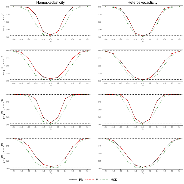
Figure 1: Power of tests with $(n,p_{x},p_{z})=(150,50,10)$ under 5% level over 1000 simulations. “MCD” represents the modified Craig–Donald test test by Kolesár, (2018). The nominal size 0.05 and power 1 are shown by the horizontal dashed lines.

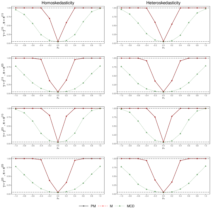
Figure 2: Power of tests with $(n,p_{x},p_{z})=(500,450,10)$ under 5% level over 1000 simulations. “MCD” represents the modified Craig–Donald test test by Kolesár, (2018). The nominal size 0.05 and power 1 are shown by the horizontal dashed lines.

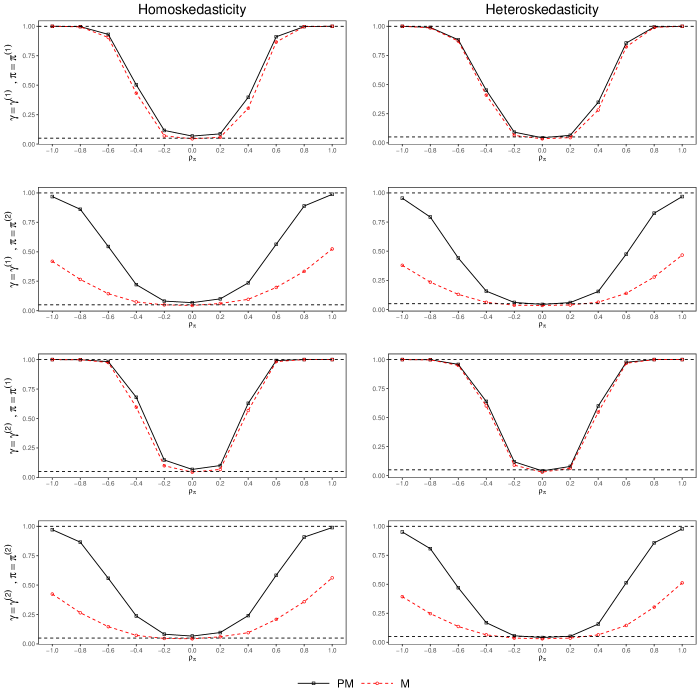
Figure 3: Power of tests with $(n,p_{x},p_{z})=(150,50,100)$ under 5% level over 1000 simulations. The nominal size 0.05 and power 1 are shown by the horizontal dashed lines.

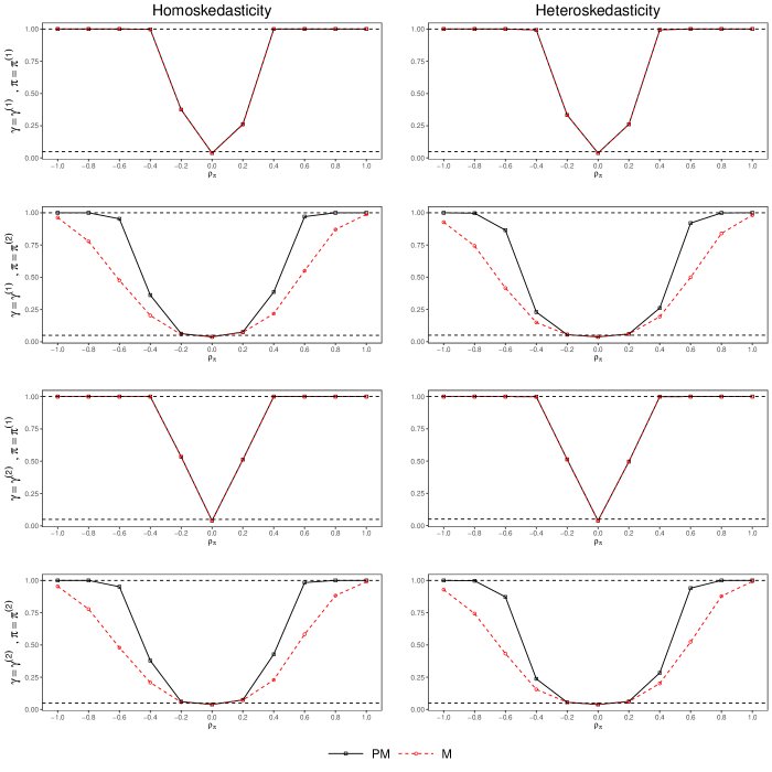
Figure 4: Power of tests with $(n,p_{x},p_{z})=(500,450,100)$ under 5% level over 1000 simulations. The nominal size 0.05 and power 1 are shown by the horizontal dashed lines.

5 Empirical Example

Table 2: Descriptive Statistics of the Raw Data.

Notation	Variable Name	Min	Median	Max	Mean	Std. Dev.
$Y$	Log GDP	7.463	10.422	12.026	10.184	1.102
$D$	Trade	0.098	0.758	4.129	0.869	0.520
$X_{1}$	Log Population	-3.037	1.472	6.674	1.355	1.830
$X_{2}$	Log Area	5.193	11.958	16.611	11.685	2.312
$Z_{1}$	$\widehat{T}$	0.015	0.079	0.297	0.092	0.052
$Z_{2}$	Languages	1.000	1.000	16.000	1.887	2.129
$Z_{3}$	Water Area	0.000	2340.000	891163.000	25218.771	100518.984
$Z_{4}$	Land Boundaries	0.000	1881.000	22147.000	2819.987	3404.441
$Z_{5}$	% Forest	0.000	30.319	98.258	29.713	22.416
$Z_{6}$	Arable Land	0.558	42.035	82.560	40.760	21.611
$Z_{7}$	Coast	0.000	515.000	202080.000	4242.147	17399.583
$Z_{8}$	$Z_{1}\cdot Z_{2}$	0.017	0.113	1.480	0.170	0.199
$Z_{9}$	$Z_{1}\cdot Z_{3}$	0.000	201.263	87556.265	1872.710	8160.430
$Z_{10}$	$Z_{1}\cdot Z_{4}$	0.000	184.863	2231.550	242.217	287.270
$Z_{11}$	$Z_{1}\cdot Z_{5}$	0.000	1.946	20.573	2.686	3.025
$Z_{12}$	$Z_{1}\cdot Z_{6}$	0.033	3.099	19.408	3.802	3.112
$Z_{13}$	$Z_{1}\cdot Z_{7}$	0.000	39.891	19854.247	352.687	1675.864
$Z_{14}$	PM2.5	5.861	22.252	99.734	27.868	19.436
$Z_{15}$	Access to Electricity	9.300	99.800	100.000	84.434	26.245
$Z_{16}$	Ease of Doing Business Index	1.000	85.000	188.000	88.356	54.022

To illustrate the usefulness of the proposed test with high-dimensional data, we revisit the empirical analysis of the effect of trade on economic growth (Frankel and Romer,, 1999, FR99 hereafter). Fan and Zhong, (2018) searched for instruments (all geographical variables) following the celebrated gravity theory of trade. In this paper, we update all data to 2018 and expand the set of IVs from Fan and Zhong, (2018) to include potentially invalid IVs from World Bank economic data. Following the literature, the outcome $Y$ is the logarithm of GDP. There are $n=159$ countries, and $p=p_{z}+p_{x}=58$, which includes (1) the constructed trade $\widehat{T}$ proposed by FR99 under the guidance of the gravity theory of trade, (2) the logarithms of population $X_{1}$ and land area describing the sizes of the countries $X_{2}$ and (3) other covariates and candidate IVs concerning geographical characteristics, energy, the environment and natural resources, and business activity variables. The outcome variable, the endogenous variable, the original FR99 covariates, and a subset of the baseline instruments used in Fan and Zhong, (2018), together with three additional and possibly invalid IVs, are summarized in Table 2. We perform overidentification tests using this (sub)set of IVs.

Table 3: P-values of different tests.

Instrument Sets	MCD	M	PM
$\{Z_{1},Z_{2},\cdots,Z_{16}\}$	0.062	0.029	0.000
$\{Z_{1},Z_{2},\cdots,Z_{13}\}$	0.317	0.275	0.275

We standardize the data so that all variables have zero sample mean and unit standard deviation and then compare the results of different testing methods. Table 3 shows the p values of different tests performed on the real data. We first test the correct specifications of all 16 instruments in Table 2 and expect the null hypothesis to be rejected since at least some of the instruments $Z_{14}$ (about climate), $Z_{15}$ (about resources) and $Z_{16}$ (about business activity) are likely to have a direct effect on economic growth. We can see that the M test and PM test reject the null hypothesis at the 5% and 1% levels, respectively, while MCD fails to reject the validity of IVs at the 5% level.

As mentioned earlier, empirical researchers can also use our method to test whether a subset of IVs is valid. Here, we select the subset of IVs used in Fan and Zhong, (2018), including $Z_{1},Z_{2},\cdots,Z_{13}$, as displayed in Table 2, and treat the other instruments as covariates. Therefore, the variable dimensions are now $p_{x}=45$ and $p_{z}=13$. All the considered tests do not reject the null hypothesis, meaning there is no evidence that this subset of instruments is invalid.

The takeaway from this empirical exercise is that practitioners should be cautious in the interpretation of a failure to reject the null hypothesis by existing overidentification tests such as MCD when many covariates and/or instruments are present. Using tests with low power would result in further difficulty in the estimation and inference of the endogenous treatment effect. Our proposed test improves the power in different model settings; hence, it is recommended in a data-rich environment to detect invalid instruments.

6 Conclusion

In this paper, we develop a new test on overidentifying restrictions for linear IV models with high-dimensional covariates and/or IVs. This test is robust to heteroskedasticity. We show that under sparsity, our PM test has better theoretical power than the existing $\chi^{2}$-type tests while having the size under control, even when $p>n$. The higher power stems from the utilization of a sparse model structure. This substantially improves the empirical power against many locally invalid instruments. The procedure can be used to test any overidentifying restrictions of a subset. As high-dimensional data become more common in observational studies, the PM test should have many applications in detecting instrument misspecifications. From a technical perspective, this paper extends the inference of maximum and $L_{2}$ norms, allowing for heteroskedasticity, and shows applicability to triangular systems such as the linear IV regression model. We would like to pursue the theoretical discussion of many locally invalid IVs in the future.

Appendices to “A Heteroskedastic-Robust Overidentifying Restriction Test with High-Dimensional Covariates”

The Appendices include the following parts: Section A provides additional details and examples. Section B contains all technical proofs. Section C collects the omitted simulation results from the main text.

A Additional Details and Discussions

A.1 The CLIME Procedure

Define the CLIME estimator (Cai et al.,, 2011) as

$$\widehat{\Omega} =(\widehat{\Omega}_{jk})_{j,k\in[p]}\text{ where }\widehat{\Omega}_{jk}=\widehat{\Omega}_{jk}^{(1)}\boldsymbol{1}(|\widehat{\Omega}_{jk}^{(1)}|\leq|\widehat{\Omega}_{kj}^{(1)}|)+\widehat{\Omega}_{kj}\boldsymbol{1}(|\widehat{\Omega}_{jk}^{(1)}|>|\widehat{\Omega}_{kj}^{(1)}|),$$ (A1)

$$\widehat{\Omega}^{(1)} =(\widehat{\Omega}^{(1)}_{1},\widehat{\Omega}^{(1)}_{2},\cdots,\widehat{\Omega}^{(1)}_{n}),$$

$$\widehat{\Omega}^{(1)}_{j} =\arg\min_{\omega\in\mathbb{R}^{p}}\|\omega\|_{1},\ \text{s.t. }\|\widehat{\Sigma}\omega-\delta_{j}\|_{\infty}\leq\mu_{\omega},$$

where $\delta_{j}$ denotes the $j$-th standard basis of $\mathbb{R}^{p}$ whose components are all zero except the $j$-th equaling one, and $\mu_{\omega}$ is a positive tuning parameter satisfying Assumption 5(ii). The restriction to solve $\widehat{\Omega}^{(1)}$ controls the estimation error, and the transformation from $\widehat{\Omega}^{(1)}$ to $\widehat{\Omega}$ is for symmetry such that $\widehat{\Omega}_{jk}=\widehat{\Omega}_{kj}$. Lemma B4 provides the convergence rates of the CLIME estimator specified by (A1).

A.2 Relation between $\pi$ and $\pi_{A}$

As discussed in Section 3 of the paper, the true $\pi$ is of our interest while we work with the data scale-invariant version of $\pi_{A}$ (or $\pi_{A^{*}}$). It is thus helpful to look into the relation between $\pi$ and the identified $\pi_{A^{*}}$ for a clearer picture of the alternative set $\mathcal{H}_{M}(t)$ defined as (32). Below are several illustrative examples. Example 1 shows that perfectly parallel $\pi$ and $\gamma$ cause zero $\pi_{A^{*}}$ even if $\pi\neq 0$, and hence the M test, as well as all other overidentification tests, has no power against invalid IVs. Example 2 shows that when $\pi$ and $\gamma$ are far away from perfectly parallel, the alternative set defined by $\|{A^{*}}^{1/2}\pi_{A^{*}}\|_{\infty}$ is similar to that defined by $\|{A^{*}}^{1/2}\pi\|_{\infty}$ under sparsity.

Example 1.

Recall that the discussions from (19) to (20) illustrate the absence of power when $\pi$ and $\gamma$ are perfectly parallel. A trivial example is $p_{z}=1$ which obviously is not overidentified. Another example with $p_{z}=2$ is given as follows. For simplicity, let $A^{*}=I_{2}$, $\pi=\rho_{\pi}(1,1)^{\top}$ and $\gamma=(1,1)^{\top}$. Here $|\rho_{\pi}|$ measures the strength of IV invalidity. Then it is easy to compute the $\pi_{A*}=\pi-\gamma(\pi^{\top}\gamma/\gamma^{\top}\gamma)=0$ for any $\rho_{\pi}\in\mathbb{R}$.

Example 2.

Recall that ${\rm R}_{A^{*}}(\gamma,\pi)$ is defined as (31). Following the same arguments from (19) to (20), as $|{\rm R}_{A^{*}}(\gamma,\pi)|$ is strictly bounded away from one, we have ${\rm Q}_{A^{*}}(\pi)\asymp{\rm Q}_{A^{*}}(\pi_{A^{*}})$. Hence, when $A^{*}$ is diagonal,

$$\|A^{*1/2}\pi\|_{\infty}\lesssim\sqrt{{\rm Q}_{A^{*}}(\pi)}\asymp\sqrt{{\rm Q}_{A^{*}}(\pi_{A^{*}})}\lesssim\sqrt{s_{\pi}+s_{\gamma}}\|A^{*1/2}\pi_{A^{*}}\|_{\infty},$$

where $s_{\pi}=\|\pi\|_{0}$ is the number of invalid IVs and $s_{\gamma}=\|\gamma\|_{0}$ is the number of relevant IVs. Consequently, $\pi\in\mathcal{H}_{M}(t)$ for some sufficiently large absolute constant $t$ whenever $\|A^{*1/2}\pi\|_{\infty}\geq t^{\prime}\sqrt{(s_{\pi}+s_{\gamma})\log p_{z}/n}$ for some absolute constant $t^{\prime}$ large enough. Following symmetric arguments, we deduce that

$$\|A^{*1/2}\pi_{A^{*}}\|_{\infty}\lesssim\sqrt{s_{\pi}}\|A^{*1/2}\pi\|_{\infty},$$

and hence any $\pi\in\mathcal{H}_{M}(t)$ implies $\|A^{*1/2}\pi\|_{\infty}\geq t^{\prime\prime}\sqrt{\log p_{z}/(ns_{\pi})}$ for some $t^{\prime\prime}$. Hence, when $\pi$ and $\gamma$ are not perfectly correlated and $s_{\pi}=\|\pi\|_{0}$ is small, the alternative set induced by $\|A^{*}\pi_{A^{*}}\|_{\infty}$ as (32) is almost equivalent to that induced by $\|A^{*}\pi\|_{\infty}$.

In summary, the alternative set induced by the data scale-invariant version of $\pi_{A^{*}}$ can fulfill the task of testing the validity of IVs measured by $\pi$.

B Proofs

Throughout the proof, we use $C$ and $c$ to denote generic absolute constants that may vary from place to place. We first present some useful preliminary lemmas in Section B.1. Section B.2 includes the proofs of the theoretical results in Section 2 of the main text. Firstly, some essential propositions about the initial Lasso estimators and test statistics are summarized in Section B.2.1. Secondly, we give the proof of Theorem 1 in Section B.2.2. Section B.3 includes the proofs of the main theoretical results of the proposed tests in Section 3 of the main text. Firstly, some essential propositions are given in Section B.3.1. Secondly, we give the proofs of Theorems 2 and 3 in Sections B.3.2 and B.3.3, respectively.

B.1 Preliminary Lemmas

This subsection provides useful lemmas implied by (or directly from) other literature.

Define the restricted eigenvalue of the empirical Gram matrix $\widehat{\Sigma}=W^{\top}W/n$, given as

$$\kappa(\widehat{\Sigma},s)=\inf_{\theta\in\mathcal{R}(s)}\dfrac{\theta^{\top}\widehat{\Sigma}\theta}{\|\theta\|_{2}^{2}},$$ (B2)

where the restricted set $\mathcal{R}(s):=\{\theta\in\mathbb{R}^{p}:\|\theta_{\mathcal{M}^{c}}\|_{1}\leq 3\|\theta_{\mathcal{M}}\|_{1}\text{ for all }\mathcal{M}\subset\mathbb{R}^{p}\text{ and }|\mathcal{M}|\leq s\}$. Lemma B1 provides the Lasso convergence rate. This is a direct result of Lemma 1 in Mei and Shi, (2022) and Theorem 6.1 of Bühlmann and van de Geer, (2011).

Lemma B1.

Suppose that $4\|n^{-1}W^{\top}\varepsilon_{j}\|_{\infty}\leq\lambda_{jn}$ for $j=1,2$. Then

$$\max\{\|\widehat{\Gamma}-\Gamma\|_{2},\|\widehat{\gamma}-\gamma\|_{2},\|\widehat{\Psi}-\Psi\|_{2},\|\widehat{\psi}-\psi\|_{2}\} \lesssim\dfrac{\sqrt{s}\lambda_{n}}{\kappa(\widehat{\Sigma},s)},$$ (B3)

$$\max\{\|\widehat{\Gamma}-\Gamma\|_{1},\|\widehat{\gamma}-\gamma\|_{1},\|\widehat{\Psi}-\Psi\|_{1},\|\widehat{\psi}-\psi\|_{1}\} \lesssim\dfrac{s\lambda_{n}}{\kappa(\widehat{\Sigma},s)}.$$

with $\lambda_{n}=\max(\lambda_{1n},\lambda_{2n})$. In addition, if $4\|n^{-1}W^{\top}{\mathchoice{{\ooalign{\hbox{\raise 6.25pt\hbox{\scalebox{1.0}[-1.0]{\lower 6.25pt\hbox{$\displaystyle\widehat{\vrule width=0.0pt,height=4.30554pt\vrule height=0.0pt,width=4.65627pt}$}}}}\cr\hbox{$\displaystyle e$}}}}{{\ooalign{\hbox{\raise 6.25pt\hbox{\scalebox{1.0}[-1.0]{\lower 6.25pt\hbox{$\textstyle\widehat{\vrule width=0.0pt,height=4.30554pt\vrule height=0.0pt,width=4.65627pt}$}}}}\cr\hbox{$\textstyle e$}}}}{{\ooalign{\hbox{\raise 5.81944pt\hbox{\scalebox{1.0}[-1.0]{\lower 5.81944pt\hbox{$\scriptstyle\widehat{\vrule width=0.0pt,height=3.01389pt\vrule height=0.0pt,width=3.25938pt}$}}}}\cr\hbox{$\scriptstyle e$}}}}{{\ooalign{\hbox{\raise 5.53241pt\hbox{\scalebox{1.0}[-1.0]{\lower 5.53241pt\hbox{$\scriptscriptstyle\widehat{\vrule width=0.0pt,height=2.15277pt\vrule height=0.0pt,width=2.32813pt}$}}}}\cr\hbox{$\scriptscriptstyle e$}}}}}_{A}\|_{\infty}\leq\lambda_{3n}$,

$$\max\{\|\widehat{\pi}_{A}-{\mathchoice{{\ooalign{\hbox{\raise 6.25pt\hbox{\scalebox{1.0}[-1.0]{\lower 6.25pt\hbox{$\displaystyle\widehat{\vrule width=0.0pt,height=4.30554pt\vrule height=0.0pt,width=5.70027pt}$}}}}\cr\hbox{$\displaystyle\pi$}}}}{{\ooalign{\hbox{\raise 6.25pt\hbox{\scalebox{1.0}[-1.0]{\lower 6.25pt\hbox{$\textstyle\widehat{\vrule width=0.0pt,height=4.30554pt\vrule height=0.0pt,width=5.70027pt}$}}}}\cr\hbox{$\textstyle\pi$}}}}{{\ooalign{\hbox{\raise 5.81944pt\hbox{\scalebox{1.0}[-1.0]{\lower 5.81944pt\hbox{$\scriptstyle\widehat{\vrule width=0.0pt,height=3.01389pt\vrule height=0.0pt,width=3.99019pt}$}}}}\cr\hbox{$\scriptstyle\pi$}}}}{{\ooalign{\hbox{\raise 5.53241pt\hbox{\scalebox{1.0}[-1.0]{\lower 5.53241pt\hbox{$\scriptscriptstyle\widehat{\vrule width=0.0pt,height=2.15277pt\vrule height=0.0pt,width=2.85013pt}$}}}}\cr\hbox{$\scriptscriptstyle\pi$}}}}}_{A}\|_{2},\|\widehat{\varphi}_{A}-{\mathchoice{{\ooalign{\hbox{\raise 6.25pt\hbox{\scalebox{1.0}[-1.0]{\lower 6.25pt\hbox{$\displaystyle\widehat{\vrule width=0.0pt,height=4.30554pt\vrule height=0.0pt,width=6.54167pt}$}}}}\cr\hbox{$\displaystyle\varphi$}}}}{{\ooalign{\hbox{\raise 6.25pt\hbox{\scalebox{1.0}[-1.0]{\lower 6.25pt\hbox{$\textstyle\widehat{\vrule width=0.0pt,height=4.30554pt\vrule height=0.0pt,width=6.54167pt}$}}}}\cr\hbox{$\textstyle\varphi$}}}}{{\ooalign{\hbox{\raise 5.81944pt\hbox{\scalebox{1.0}[-1.0]{\lower 5.81944pt\hbox{$\scriptstyle\widehat{\vrule width=0.0pt,height=3.01389pt\vrule height=0.0pt,width=4.57916pt}$}}}}\cr\hbox{$\scriptstyle\varphi$}}}}{{\ooalign{\hbox{\raise 5.53241pt\hbox{\scalebox{1.0}[-1.0]{\lower 5.53241pt\hbox{$\scriptscriptstyle\widehat{\vrule width=0.0pt,height=2.15277pt\vrule height=0.0pt,width=3.27083pt}$}}}}\cr\hbox{$\scriptscriptstyle\varphi$}}}}}_{A}\|_{2}\} \lesssim\dfrac{\sqrt{s}\lambda_{3n}}{\kappa(\widehat{\Sigma},s)},$$ (B4)

$$\max\{\|\widehat{\pi}_{A}-{\mathchoice{{\ooalign{\hbox{\raise 6.25pt\hbox{\scalebox{1.0}[-1.0]{\lower 6.25pt\hbox{$\displaystyle\widehat{\vrule width=0.0pt,height=4.30554pt\vrule height=0.0pt,width=5.70027pt}$}}}}\cr\hbox{$\displaystyle\pi$}}}}{{\ooalign{\hbox{\raise 6.25pt\hbox{\scalebox{1.0}[-1.0]{\lower 6.25pt\hbox{$\textstyle\widehat{\vrule width=0.0pt,height=4.30554pt\vrule height=0.0pt,width=5.70027pt}$}}}}\cr\hbox{$\textstyle\pi$}}}}{{\ooalign{\hbox{\raise 5.81944pt\hbox{\scalebox{1.0}[-1.0]{\lower 5.81944pt\hbox{$\scriptstyle\widehat{\vrule width=0.0pt,height=3.01389pt\vrule height=0.0pt,width=3.99019pt}$}}}}\cr\hbox{$\scriptstyle\pi$}}}}{{\ooalign{\hbox{\raise 5.53241pt\hbox{\scalebox{1.0}[-1.0]{\lower 5.53241pt\hbox{$\scriptscriptstyle\widehat{\vrule width=0.0pt,height=2.15277pt\vrule height=0.0pt,width=2.85013pt}$}}}}\cr\hbox{$\scriptscriptstyle\pi$}}}}}_{A}\|_{1},\|\widehat{\varphi}_{A}-{\mathchoice{{\ooalign{\hbox{\raise 6.25pt\hbox{\scalebox{1.0}[-1.0]{\lower 6.25pt\hbox{$\displaystyle\widehat{\vrule width=0.0pt,height=4.30554pt\vrule height=0.0pt,width=6.54167pt}$}}}}\cr\hbox{$\displaystyle\varphi$}}}}{{\ooalign{\hbox{\raise 6.25pt\hbox{\scalebox{1.0}[-1.0]{\lower 6.25pt\hbox{$\textstyle\widehat{\vrule width=0.0pt,height=4.30554pt\vrule height=0.0pt,width=6.54167pt}$}}}}\cr\hbox{$\textstyle\varphi$}}}}{{\ooalign{\hbox{\raise 5.81944pt\hbox{\scalebox{1.0}[-1.0]{\lower 5.81944pt\hbox{$\scriptstyle\widehat{\vrule width=0.0pt,height=3.01389pt\vrule height=0.0pt,width=4.57916pt}$}}}}\cr\hbox{$\scriptstyle\varphi$}}}}{{\ooalign{\hbox{\raise 5.53241pt\hbox{\scalebox{1.0}[-1.0]{\lower 5.53241pt\hbox{$\scriptscriptstyle\widehat{\vrule width=0.0pt,height=2.15277pt\vrule height=0.0pt,width=3.27083pt}$}}}}\cr\hbox{$\scriptscriptstyle\varphi$}}}}}_{A}\|_{1}\} \lesssim\dfrac{s\lambda_{3n}}{\kappa(\widehat{\Sigma},s)}.$$

Lemma B2 shows the probability bounds for the maximum norm of some sub-Gaussian and sub-exponential variables, and a lower bound of the restricted eigenvalue useful in the proofs.

Lemma B2.

Under Assumptions 1-2,

$$\max_{i\in[n],j\in[p]}|W_{ij}| \lesssim_{p}\sqrt{\log p+\log n}.$$ (B5)

When $\log p=o(n)$,

$$\|\widehat{\Sigma}-\Sigma\|_{\infty} \lesssim_{p}\sqrt{\dfrac{\log p}{n}},$$ (B6)

$$\|n^{-1}W^{\top}\varepsilon_{j}\|_{\infty} \lesssim_{p}\sqrt{\dfrac{\log p}{n}},\text{ for }j=1,2.$$ (B7)

Besides, when $s=o(\sqrt{n/\log p})$, w.p.a.1

$$\kappa(\widehat{\Sigma},s)\geq 0.5c_{\Sigma}.$$ (B8)

Proof of Lemma B2.

By Assumption 1, (B5) is the result of

$$\Pr\left(\max_{i\in[n],j\in[p]}|W_{ij}|>\sqrt{2c^{-1}\cdot\log(np)}\right)\leq np\cdot C{\rm e}^{-2\log(np)}=C(np)^{-1}\to 0.$$

In terms of (B6) and (B7), the LHS of the inequalities is the maximum norm of sub-exponential vectors with mean zero. By Corollary 5.17 in Vershynin, (2010), when $\log p=o(n)$ there exists some $c>0$ such that

$$\Pr\left(\|\widehat{\Sigma}-\Sigma\|_{\infty}>\sqrt{2\log p/(cn)}\right)\leq 2p\cdot\exp(-2\log p)\to 0,$$

and similar probability bound holds for $n^{-1}W^{\top}\varepsilon_{j}$. As for (B8), for any $\theta\in\mathcal{R}$

$$\theta^{\top}\widehat{\Sigma}\theta \geq\theta^{\top}\Sigma\theta-\left|\theta^{\top}(\widehat{\Sigma}-\Sigma)\theta\right|$$

$$\geq c_{\Sigma}\theta^{\top}\theta-\|\theta\|_{1}^{2}\|\widehat{\Sigma}-\Sigma\|_{\infty}$$

$$\geq c_{\Sigma}\|\theta\|_{2}^{2}-(\|\theta_{\mathcal{M}}\|_{1}+\|\theta_{\mathcal{M}^{c}}\|_{1})^{2}\cdot c\sqrt{\dfrac{\log p}{n}}$$

$$\geq c_{\Sigma}\|\theta\|_{2}^{2}-(4\|\theta_{\mathcal{M}}\|_{`})^{2}c\sqrt{\dfrac{\log p}{n}}$$

$$\geq c_{\Sigma}\|\theta\|_{2}^{2}-16c\cdot s\sqrt{\dfrac{\log p}{n}}\cdot\|\theta\|_{2}^{2}\geq 0.5c_{\Sigma}\|\theta\|_{2}^{2},$$

for some absolute constant $c>0$, where the last inequality applies $s=o(\sqrt{n/\log p})$. ∎

Lemma B3 shows that under certain conditions, linear transformations of sub-Gaussian vectors are still sub-Gaussian.

Lemma B3.

Suppose that all entries in the vector $x=(x_{1},x_{,}\cdots,x_{p})^{\top}\in\mathbb{R}^{p}$ are centered sub-Gaussian variables such that $\mathbb{E}(x)=0$ and for any $\mu\in\mathbb{R}$, $\max_{j\in[p]}\Pr(|x_{j}|>\mu)\leq C\exp(-c\mu^{2})$ for some absolute constants $C$ and $c$. If there exists some matrix $B\in\mathbb{R}^{p\times p}$ such that $\|B\|_{2}\leq C_{B}$, then the entries in the $p\times 1$ vector $Bx$ are sub-Gaussian such that $\max_{j\in[p]}\Pr(|(Bx)_{j}|>\mu)\leq C_{B}^{\prime}\exp(-c_{B}^{\prime}\mu^{2})$ with some absolute constants $C_{B}^{\prime}$ and $c_{B}^{\prime}$.

Proof of Lemma B3.

By the equivalence between Conditions 1 and 2 in Lemma 5.5 of Vershynin, (2010), we know that $\max_{j\in[p]}\Pr(|(Bx)_{j}|>\mu)\leq C_{B}^{\prime}\exp(-c_{B}^{\prime}\mu^{2})$ is equivalent to the fact that the sub-Gaussian norm

$$\max_{j\in p}\sup_{d\in\mathbb{N}}d^{-1/2}(\mathbb{E}|x_{j}|^{d})^{1/d},$$ (B9)

is bounded by some absolute constant $K$. Let $B_{jk}$ denote the $(j,k)$-th element of $B$. By Proposition 5.10 of the same reference,

$$\Pr(|(Bx)_{j}|>\mu)=\Pr\left(|\sum_{k=1}^{p}B_{jk}x_{k}|>\mu\right)\leq\exp\left(1-\dfrac{c\mu^{2}}{K^{2}\sum_{k=1}^{p}B_{jk}^{2}}\right)\leq\exp\left(1-\dfrac{c\mu^{2}}{K^{2}C_{B}^{2}}\right),$$

for some absolute constant $c$, and Lemma B3 follows with $C_{B}^{\prime}={\rm e}$ and $c_{B}^{\prime}=c/(KC_{B})^{2}$. ∎

Lemma B4 shows the asymptotic properties of the inverse covariance estimator CLIME (A1).

Lemma B4.

Under Assumptions 1-3 and 5,

$$\|\widehat{\Omega}\|_{1}\leq m_{\omega},$$ (B10)

w.p.a.1. Besides,

$$\|\widehat{\Omega}-\Omega\|_{1}\lesssim_{p}s_{\omega}\cdot m_{\omega}^{2-2q}\left(\dfrac{\log p}{n}\right)^{(1-q)/2},$$ (B11)

$$\|\widehat{\Sigma}\widehat{\Omega}-I\|_{\infty}\lesssim_{p}s_{\omega}\cdot m_{\omega}^{2-2q}\left(\dfrac{\log p}{n}\right)^{(1-q)/2}.$$ (B12)

Proof of Lemma B4.

By Lemma B3, each element of $X\Omega^{1/2}$ is sub-Gaussian with uniformly bounded sub-Gaussian norm defined as (B9). By Lemma 23 in Javanmard and Montanari, (2014), $\Omega$ is a feasible solution w.p.a.1. in (A1) when $\mu_{\omega}=C\sqrt{\log p/n}$ with some sufficiently large absolute constant $C$, i.e. $\|\widehat{\Sigma}\Omega-I_{p}\|_{\infty}\leq\mu_{\omega}$ w.p.a.1. By the definition of $\widehat{\Omega}$ in (A1)

$$\|\widehat{\Omega}\|_{1}\leq\|\widehat{\Omega}^{(1)}\|_{1}\leq\|\Omega\|_{1}\leq m_{\omega}$$

w.p.a.1, which verifies (B10). Besides,

$$\|\widehat{\Omega}-\Omega\|_{\infty}\leq\|\widehat{\Omega}^{(1)}-\Omega\|_{\infty} \leq\|\Omega\|_{1}\|\Sigma\widehat{\Omega}^{(1)}-I_{p}\|_{\infty}$$

$$\leq m_{\omega}\left(\|(\widehat{\Sigma}-\Sigma)(\widehat{\Omega}^{(1)}-\Omega)\|_{\infty}+\|\widehat{\Sigma}(\widehat{\Omega}^{(1)}-\Omega)\|_{\infty}\right)$$

$$\leq m_{\omega}\left((\|\widehat{\Omega}^{(1)}\|_{1}+\|\Omega\|_{1})\cdot\|\widehat{\Sigma}-\Sigma\|_{\infty}+\|\widehat{\Sigma}\widehat{\Omega}^{(1)}-I_{p}\|_{\infty}+\|\widehat{\Sigma}\Omega-I_{p}\|_{\infty}\right)$$

$$\lesssim_{p}m_{\omega}^{2}\sqrt{\dfrac{\log p}{n}}.$$

Following the proof of (14) in Theorem 6 of Cai et al., (2011) we can deduce

$$\|\widehat{\Omega}-\Omega\|_{1}\lesssim_{p}s_{\omega}\cdot(\|\widehat{\Omega}-\Omega\|_{\infty})^{1-q}\lesssim_{p}s_{\omega}m_{\omega}^{2-2q}\left(\dfrac{\log p}{n}\right)^{(1-q)/2},$$

which is (B11). For (B12),

$$\|\widehat{\Sigma}\widehat{\Omega}-I\|_{\infty} \leq\|\widehat{\Sigma}\Omega-I\|_{\infty}+\|\widehat{\Sigma}(\widehat{\Omega}-\Omega)\|_{\infty}$$

$$\lesssim_{p}\sqrt{\dfrac{\log p}{n}}+\|\widehat{\Sigma}\|_{\infty}\|\widehat{\Omega}-\Omega|\|_{1}$$

$$\lesssim_{p}\sqrt{\dfrac{\log p}{n}}+(\|\widehat{\Sigma}-\Sigma\|_{\infty}+\|\Sigma\|_{\infty})\cdot s_{\omega}\cdot m_{\omega}^{2-2q}\left(\dfrac{\log p}{n}\right)^{(1-q)/2}$$

$$\lesssim_{p}s_{\omega}\cdot m_{\omega}^{2-2q}\left(\dfrac{\log p}{n}\right)^{(1-q)/2}.$$

The proof of Lemma B4 completes. ∎

Lemma B5 shows a more convenient asymptotic regime used in the proofs.

Lemma B5.

Under Assumption 4

$$\dfrac{m_{\omega}^{3}s^{3/2}(\log p)^{(7+\nu)/2}}{\sqrt{n}}=o(1\wedge\|\gamma\|_{2}).$$ (B13)

Proof of Lemma B5.

By Assumption 4, we have

$$\left(\dfrac{m_{\omega}^{3}s^{3/2}(\log p)^{(7+\nu)/2}}{n^{1/2}}\right)^{1-q}=\dfrac{m_{\omega}^{3-3q}s^{(3-3q)/2}(\log p)^{[(7+\nu)(1-q)]/2}}{n^{(1-q)/2}}\leq\dfrac{m_{\omega}^{3-2q}s^{(3-q)/2}(\log p)^{(7+\nu-q)/2}}{n^{(1-q)/2}}=o(1\wedge\|\gamma\|_{2}).$$

By $0\leq q<1$ and $\left(\dfrac{m_{\omega}^{3}s^{3/2}(\log p)^{(7+\nu)/2}}{n^{1/2}}\right)^{1-q}<1$ with $n$ large enough, we have

$$\dfrac{m_{\omega}^{3}s^{3/2}(\log p)^{(7+\nu)/2}}{n^{1/2}}<\left(\dfrac{m_{\omega}^{3}s^{3/2}(\log p)^{(7+\nu)/2}}{n^{1/2}}\right)^{1-q}=o(1\wedge\|\gamma\|_{2}),$$

as $n\to\infty$. ∎

Lemma B6 shows the probability bounds for the maximum norms that are useful to bound the estimation errors of asymptotic variance.

Lemma B6.

Under Assumptions 1, 2 and 4,

$$\max_{j,k,\ell,m\in[p]}\left|\dfrac{1}{n}\sum_{i=1}^{n}W_{ij}W_{ik}W_{i\ell}W_{im}-\dfrac{1}{n}\sum_{i=1}^{n}\mathbb{E}\left(W_{ij}W_{ik}W_{i\ell}W_{im}\right)\right|\lesssim_{p}\sqrt{\dfrac{\log p}{n}},$$ (B14)

$$\max_{j,k,h\in[p]}\left|\dfrac{1}{n}\sum_{i=1}^{n}W_{ij}W_{ik}W_{ih}\varepsilon_{im}\right|\lesssim_{p}\sqrt{\dfrac{\log p}{n}},$$ (B15)

and

$$\max_{j,k\in[p]}\left|\dfrac{1}{n}\sum_{i=1}^{n}W_{ij}W_{ik}\left(\varepsilon_{i\ell}\varepsilon_{im}-\mathbb{E}[\varepsilon_{i\ell}\varepsilon_{im}|W]\right)\right|\lesssim_{p}\sqrt{\dfrac{\log p}{n}},$$ (B16)

for $\ell,m=1,2$.

Proof of Lemma B6.

We only show (B14). The other two inequalities can be verified following the same procedures. By Assumption 1, for any $j,k,\ell,m\in[p]$, we know that

$$\Pr(|W_{ij}W_{ik}W_{i\ell}W_{im}|>\mu)\leq C\exp(-c\mu^{0.5}),$$

for some absolute constants $C$ and $c$. By Theorem 1 of Merlevède et al., (2011), we know that for any $\mu>0$

$$\ \ \Pr\left(\left|\sum_{i=1}^{n}\left(W_{ij}W_{ik}W_{i\ell}W_{im}-\mathbb{E}(W_{ij}W_{ik}W_{i\ell}W_{im})\right)\right|>\mu\right)$$

$$\leq n\exp\left(-\dfrac{\mu^{r}}{C_{1}}\right)+\exp\left(-\dfrac{\mu^{2}}{C_{2}(1+nV)}\right)+\exp\left(-\dfrac{\mu^{2}}{C_{3}n}\exp\left(\dfrac{\mu^{r(1-r)}}{C_{4}(\log\mu)^{r}}\right)\right),$$

where $r=\left(\dfrac{1}{0.5}+\dfrac{1}{r_{2}}\right)^{-1}<1$ as defined in (2.8) of the same paper. Here $1/r_{2}$ measures an upper bound of the mixing coefficient for a time series, which can be arbitrarily small for independent data. Taking $\mu=\sqrt{C_{x}n\log p}$ with $C_{x}=(2C_{1})^{2/r}\vee(5C_{2}V)$. Then

$$\ \ \Pr\left(\max_{j,k,\ell,m\in[p]}\left|\dfrac{1}{n}\sum_{i=1}^{n}\left(W_{ij}W_{ik}W_{i\ell}W_{im}-\mathbb{E}(W_{ij}W_{ik}W_{i\ell}W_{im})\right)\right|>\sqrt{\dfrac{C_{x}\log p}{n}}\right)$$

$$\leq np^{4}\exp\left(-\dfrac{(C_{x}n\log p)^{r/2}}{C_{1}}\right)+p^{4}\exp\left(-\dfrac{C_{x}n\log p}{C_{2}(1+nV)}\right)+$$

$$\ \ \ \ p^{4}\exp\left(-\dfrac{C_{x}n\log p}{C_{3}n}\exp\left(\dfrac{(C_{x}n\log p)^{r(1-r)/2}}{C_{4}(0.5\log(C_{x}n\log p))^{r}}\right)\right)$$

$$\leq np^{4}\exp\left(-2(n\log p)^{r/2}\right)+p^{4}\exp(-5\log p)+o(1)$$

$$\leq\exp\left(-(2(n\log p)^{r/2}-\log n-\log p)\right)+o(1),$$

where the second inequality applies that

$$\dfrac{(C_{x}n\log p)^{r(1-r)/2}}{C_{4}(0.5\log(C_{x}n\log p))^{r}}\to\infty.$$

Obviously, $(n\log p)^{r/2}-\log n\to\infty$. Take $r_{2}=0.5$ and hence $r=0.25$ and $2/r-1=7$. We thus also have $(n\log p)^{r/2}-\log p\to\infty$ as $(\log p)^{2/r-1}=(\log p)^{7}=o(n)$ by Lemma B5. Hence,

$$\ \ \Pr\left(\max_{j,k,\ell,m\in[p]}\left|\dfrac{1}{n}\sum_{i=1}^{n}\left(W_{ij}W_{ik}W_{i\ell}W_{im}-\mathbb{E}(W_{ij}W_{ik}W_{i\ell}W_{im})\right)\right|>\sqrt{\dfrac{C_{x}\log p}{n}}\right)=o(1),$$

and (B14) follows. ∎

B.2 Proofs of the Initial Estimator in Section 2

B.2.1 Essential Propositions

Proposition B1 provides probability upper bounds of the Lasso estimators of the reduced form estimators.

Proposition B1.

Suppose that Assumptions 1, 2 and 5 (i) hold. If $s=o(\sqrt{n/\log p})$, we have

$$\max\{\|\widehat{\Gamma}-\Gamma\|_{2},\|\widehat{\gamma}-\gamma\|_{2},\|\widehat{\Psi}-\Psi\|_{2},\|\widehat{\psi}-\psi\|_{2}\} \lesssim_{p}\sqrt{\dfrac{s\log p}{n}},$$ (B17)

$$\max\{\|\widehat{\Gamma}-\Gamma\|_{1},\|\widehat{\gamma}-\gamma\|_{1},\|\widehat{\Psi}-\Psi\|_{1},\|\widehat{\psi}-\psi\|_{1}\} \lesssim_{p}\sqrt{\dfrac{s^{2}\log p}{n}}.$$

Proof of Proposition B1.

The results are directly implied by Lemma B1, (B7) and (B8). ∎

Proposition B2 provides probability upper bounds of the weighting matrix $A$.

Proposition B2.

Suppose that Assumption 1 holds. Then

$$\|A-A^{*}\|_{2}+\|A^{1/2}-A^{*1/2}\|_{2}+\|A-A^{*}\|_{1}+\|A^{1/2}-A^{*1/2}\|_{1}\lesssim_{p}\sqrt{\dfrac{\log p}{n}}.$$ (B18)

Furthermore, when $\log p=o(n)$,

$$\|A\|_{2}+\|A^{1/2}\|_{2}+\|A\|_{1}+\|A^{1/2}\|_{1}\lesssim_{p}1.$$ (B19)

and

$$\lambda_{\min}(A)\gtrsim_{p}1.$$ (B20)

Proof of Proposition B2.

By definitions of $A$ and $A^{*}$ in (4) and (30),

$$\|A-A^{*}\|_{2}+\|A-A^{*}\|_{1}\leq 2\|\widehat{\Sigma}-\Sigma\|_{\infty}\lesssim_{p}\sqrt{\dfrac{\log p}{n}}.$$ (B21)

Hence,

$$\lambda_{\min}(A)\geq\lambda_{\min}(A^{*})-\|A-A^{*}\|_{2}\gtrsim_{p}1,$$

which verifies (B20). Besides,

$$\|A^{1/2}-A^{*1/2}\|_{2}=\|A^{1/2}-A^{*1/2}\|_{1} =\max_{j\in[p_{z}]}\left|\sqrt{n^{-1}\sum_{i=1}^{n}Z_{ij}^{2}}-\sqrt{\mathbb{E}(Z_{ij}^{2})}\right|$$

$$\leq\max_{j\in[p_{z}]}\dfrac{\left|n^{-1}\sum_{i=1}^{n}Z_{ij}^{2}-\mathbb{E}(Z_{ij}^{2})\right|}{\sqrt{n^{-1}\sum_{i=1}^{n}Z_{ij}^{2}}+\sqrt{\mathbb{E}(Z_{ij}^{2})}}$$

$$\leq\dfrac{\|\widehat{\Sigma}-\Sigma\|_{\infty}}{\sqrt{\lambda_{\min}(A)}+\sqrt{\lambda_{\min}(A^{*})}}\lesssim_{p}\sqrt{\dfrac{\log p}{n}},$$

which, together with (B21), induces (B18). Then (B19) directly follows (B18) and the result that

$$\|A^{*}\|_{2}+\|A^{*1/2}\|+\|A^{*}\|_{1}+\|A^{*1/2}\|_{1}\lesssim 1.$$

∎

Proposition B3 provides some error bounds that are useful in deriving estimation error of the asymptotic variance. Recall that $\sigma_{iA}^{2}=\sigma_{i1}^{2}-2\beta_{A}\sigma_{i12}+\beta_{A}^{2}\sigma_{i2}^{2}$. Similarly, define $\sigma_{iA^{*}}^{2}=\sigma_{i1}^{2}-2\beta_{A^{*}}\sigma_{i12}+\beta_{A}^{2}\sigma_{i2}^{2}$ where $\beta_{A^{*}}:=\dfrac{{\rm I}_{A^{*}}(\gamma,\Gamma)}{{\rm Q}_{A^{*}}(\gamma)}$ is defined below (32).

Proposition B3.

Under Assumptions 1-5, if $\pi\in\mathcal{H}_{M}(t)$ for any absolute constant $t$,

$$\left\|\dfrac{1}{n}\sum_{i=1}^{n}W_{i\cdot}W_{i\cdot}^{\top}(\sigma^{2}_{iA}-\sigma^{2}_{iA^{*}})\right\|_{\infty}+\max_{i\in[n]}|\sigma^{2}_{iA}-\sigma^{2}_{iA^{*}}|\lesssim_{p}\sqrt{\dfrac{\log p}{n}},$$ (B22)

$$\left\|\dfrac{1}{n}\sum_{i=1}^{n}W_{i\cdot}W_{i\cdot}^{\top}\sigma^{2}_{iA}\right\|_{\infty}+\max_{\ell,m\in\{1,2\}}\left\|\dfrac{1}{n}\sum_{i=1}^{n}W_{i\cdot}W_{i\cdot}^{\top}\mathbb{E}(\varepsilon_{i\ell}\varepsilon_{im}|W_{i\cdot})\right\|_{\infty}\lesssim_{p}1,$$ (B23)

$$\max_{\ell,m\in\{1,2\}}\left\|\dfrac{1}{n}\sum_{i=1}^{n}W_{i\cdot}W_{i\cdot}^{\top}\varepsilon_{i\ell}\varepsilon_{im}\right\|_{\infty}\lesssim_{p}1,$$ (B24)

$$\left\|\dfrac{1}{n}\sum_{i=1}^{n}W_{i\cdot}W_{i\cdot}^{\top}(\widehat{\varepsilon}_{i\ell}\widehat{\varepsilon}_{im}-\mathbb{E}(\varepsilon_{i\ell}\varepsilon_{im}|W))\right\|_{\infty}\lesssim_{p}\dfrac{s^{2}\log p}{n}+\sqrt{\dfrac{\log p}{n}},\text{ for }\ell,m=1,2,$$ (B25)

Proof of Proposition B3.

Proof of (B22). We first need a bound for $\beta_{A}-\beta_{A^{*}}$. Note that when $\pi\in\mathcal{H}_{M}(t)$,

$$\|\pi\|_{2}=\dfrac{\|\pi_{A^{*}}\|_{2}}{\sqrt{1-{\rm R}_{A^{*}}^{2}(\pi,\gamma)}}\asymp\|\pi_{A^{*}}\|_{2},$$ (B26)

and hence

$$\|\pi\|_{2}\lesssim\sqrt{s}\|A^{*1/2}\pi_{A^{*}}\|_{\infty}\lesssim\sqrt{\dfrac{s\log p}{n}}.$$ (B27)

Thus, by Lemma B5 $\|\pi\|_{2}\lesssim\|\gamma\|_{2}$. This implies

$$|\beta_{A^{*}}|\lesssim\dfrac{\|\Gamma\|_{2}\|\gamma\|_{2}}{\|\gamma\|_{2}^{2}}\lesssim\dfrac{\|\pi\|_{2}+|\beta|\cdot\|\gamma\|_{2}}{\|\gamma\|_{2}}\lesssim 1+\dfrac{\|\pi\|_{2}}{\|\gamma\|_{2}}\lesssim 1,$$ (B28)

and by Proposition B2

$$|{\rm I}_{A}(\gamma,\Gamma)-{\rm I}_{A^{*}}(\gamma,\Gamma)| \leq\|\Gamma\|_{2}\|A-A^{*}\|_{2}\|\gamma\|_{2}$$

$$\lesssim_{p}\|\pi+\gamma\beta\|_{2}\|\gamma\|_{2}\sqrt{\dfrac{\log p}{n}}$$

$$\lesssim\left(\|\pi\|_{2}\|\gamma\|_{2}+\|\gamma\|_{2}^{2}\right)\sqrt{\dfrac{\log p}{n}}\lesssim{\rm Q}_{A^{*}}(\gamma)\sqrt{\dfrac{\log p}{n}},$$

$$|{\rm Q}_{A}(\gamma,\Gamma)-{\rm Q}_{A^{*}}(\gamma,\Gamma)| \leq\|A-A^{*}\|_{2}\|\gamma\|_{2}^{2}\lesssim_{p}{\rm Q}_{A^{*}}(\gamma)\sqrt{\dfrac{\log p}{n}}.$$

We then deduce that

$$|\beta_{A}-\beta_{A^{*}}|=\left|\dfrac{{\rm I}_{A}(\gamma,\Gamma)-{\rm I}_{A^{*}}(\gamma,\Gamma)-\beta_{A^{*}}({\rm Q}_{A}(\gamma)-{\rm Q}_{A^{*}}(\gamma))}{{\rm Q}_{A^{*}}(\gamma)}\right|\lesssim_{p}\sqrt{\dfrac{\log p}{n}},$$ (B29)

which together with (B28) also implies

$$|\beta_{A}|\lesssim_{p}1.$$ (B30)

In addition, we have

$$|\beta_{A}^{2}-\beta_{A^{*}}^{2}|=|\beta_{A}-\beta_{A^{*}}|\cdot|\beta_{A}+\beta_{A^{*}}|\lesssim_{p}\sqrt{\dfrac{\log p}{n}}.$$ (B31)

Finally, by the boundness of $\sigma_{i2}$ defined in Assumption 2, each entry of $W_{i\cdot}\sigma_{i2}$ is also sub-Gaussian. Thus the second moment $\mathbb{E}(W_{i\cdot}W_{i\cdot}^{\top}\sigma_{i2}^{2})$ is uniformly bounded. Following the proof of (B14) we deduce that

$$\left\|\dfrac{1}{n}\sum_{i=1}^{n}\left[W_{i\cdot}W_{i\cdot}^{\top}\sigma^{2}_{i2}-\mathbb{E}(W_{i\cdot}W_{i\cdot}^{\top}\sigma_{i2}^{2})\right]\right\|_{\infty}\lesssim_{p}\sqrt{\dfrac{\log p}{n}},$$ (B32)

and hence

$$\ \ \ \ \left\|\dfrac{1}{n}\sum_{i=1}^{n}W_{i\cdot}W_{i\cdot}^{\top}\sigma^{2}_{i2}\right\|_{\infty}$$ (B33)

$$\leq\left\|\dfrac{1}{n}\sum_{i=1}^{n}W_{i\cdot}W_{i\cdot}^{\top}(\sigma^{2}_{i2}-\sigma^{2}_{i2})\right\|_{\infty}+\left\|\dfrac{1}{n}\sum_{i=1}^{n}\left[W_{i\cdot}W_{i\cdot}^{\top}\sigma^{2}_{i2}-\mathbb{E}(W_{i\cdot}W_{i\cdot}^{\top}\sigma_{i2}^{2})\right]\right\|_{\infty}+\left\|\dfrac{1}{n}\sum_{i=1}^{n}\mathbb{E}(W_{i\cdot}W_{i\cdot}^{\top}\sigma_{i2}^{2})\right\|_{\infty}$$

$$\lesssim_{p}\sqrt{\dfrac{\log p}{n}}+1\lesssim 1.$$

Similarly,

$$\left\|\dfrac{1}{n}\sum_{i=1}^{n}W_{i\cdot}W_{i\cdot}^{\top}\sigma_{i12}\right\|_{\infty}\lesssim_{p}1.$$ (B34)

Then by (B29), (B31) and (B33),

$$\begin{aligned} \left\|\dfrac{1}{n}\sum_{i=1}^{n}W_{i\cdot}W_{i\cdot}^{\top}(\sigma^{2}_{iA}-\sigma^{2}_{iA^{*}})\right\|_{\infty}&\lesssim|\beta_{A}^{2}-\beta_{A^{*}}^{2}|\cdot\left\|\dfrac{1}{n}\sum_{i=1}^{n}W_{i\cdot}W_{i\cdot}^{\top}\sigma^{2}_{i2}\right\|_{\infty}+|\beta_{A}-\beta_{A^{*}}|\cdot\left\|\dfrac{1}{n}\sum_{i=1}^{n}W_{i\cdot}W_{i\cdot}^{\top}\sigma_{i12}\right\|_{\infty}\\ &\lesssim_{p}\sqrt{\dfrac{\log p}{n}}\end{aligned},$$

and

$$\max_{i\in[n]}\left|\sigma^{2}_{iA}-\sigma^{2}_{iA^{*}}\right|_{\infty} \lesssim|\beta_{A}^{2}-\beta_{A^{*}}^{2}|\cdot\max_{i\in[n]}\sigma_{i2}^{2}+|\beta_{A}-\beta_{A^{*}}|\cdot|\max_{i\in[n]}\sigma_{i12}|\lesssim_{p}\sqrt{\dfrac{\log p}{n}}.$$

Proof of (B23). We only show the upper bound of the first term on the LHS since the second term goes through similarly. By the boundness of $\sigma_{iA^{*}}$, each entry of $W_{i\cdot}\sigma_{iA^{*}}$ is also sub-Gaussian. Thus the second moment $\mathbb{E}(W_{i\cdot}W_{i\cdot}^{\top}\sigma_{iA^{*}}^{2})$ is uniformly bounded. Following the proof of (B14) we deduce that

$$\left\|\dfrac{1}{n}\sum_{i=1}^{n}\left[W_{i\cdot}W_{i\cdot}^{\top}\sigma^{2}_{iA^{*}}-\mathbb{E}(W_{i\cdot}W_{i\cdot}^{\top}\sigma_{iA^{*}}^{2})\right]\right\|_{\infty}\lesssim_{p}\sqrt{\dfrac{\log p}{n}},$$ (B35)

and hence

$$\ \ \ \ \left\|\dfrac{1}{n}\sum_{i=1}^{n}W_{i\cdot}W_{i\cdot}^{\top}\sigma^{2}_{iA}\right\|_{\infty}$$

$$\leq\left\|\dfrac{1}{n}\sum_{i=1}^{n}W_{i\cdot}W_{i\cdot}^{\top}(\sigma^{2}_{iA}-\sigma^{2}_{iA^{*}})\right\|_{\infty}+\left\|\dfrac{1}{n}\sum_{i=1}^{n}\left[W_{i\cdot}W_{i\cdot}^{\top}\sigma^{2}_{iA^{*}}-\mathbb{E}(W_{i\cdot}W_{i\cdot}^{\top}\sigma_{iA^{*}}^{2})\right]\right\|_{\infty}+\left\|\dfrac{1}{n}\sum_{i=1}^{n}\mathbb{E}(W_{i\cdot}W_{i\cdot}^{\top}\sigma_{iA^{*}}^{2})\right\|_{\infty}$$

$$\lesssim_{p}\sqrt{\dfrac{\log p}{n}}+1\lesssim 1.$$

Proof of (B24). It immediately follows by (B16) and (B23) that

$$\ \ \ \ \left\|\dfrac{1}{n}\sum_{i=1}^{n}W_{i\cdot}W_{i\cdot}^{\top}\varepsilon_{i\ell}\varepsilon_{im}\right\|_{\infty}$$

$$\lesssim\left\|\dfrac{1}{n}\sum_{i=1}^{n}W_{i\cdot}W_{i\cdot}^{\top}\left(\varepsilon_{i\ell}\varepsilon_{im}-\mathbb{E}[\varepsilon_{i\ell}\varepsilon_{im}|W]\right)\right\|_{\infty}+\left\|\dfrac{1}{n}\sum_{i=1}^{n}W_{i\cdot}W_{i\cdot}^{\top}\mathbb{E}[\varepsilon_{i\ell}\varepsilon_{im}|W]\right\|_{\infty}$$

$$\lesssim_{p}\sqrt{\dfrac{\log p}{n}}+1\lesssim_{p}1.$$

Proof of (B25). We only prove the case with $\ell=m=1$. Other cases can be verified in the same manner. Here $\mathbb{E}(\varepsilon_{i1}^{2}|W_{i\cdot})=\sigma_{i1}^{2}$. Note that

$$\widehat{\varepsilon}_{i1}^{2}-\sigma_{i1}^{2} =\widehat{\varepsilon}_{i1}^{2}-\varepsilon_{i1}^{2}+\varepsilon_{i1}^{2}-\sigma_{i1}^{2}$$ (B36)

$$=(\widehat{\varepsilon}_{i1}-\varepsilon_{i1})^{2}+2\varepsilon_{i1}(\widehat{\varepsilon}_{i1}-\varepsilon_{i1})+\varepsilon_{i1}^{2}-\sigma_{i1}^{2}$$

$$=\left(X_{i\cdot}^{\top}(\widehat{\Psi}-\Psi)+Z_{i\cdot}^{\top}(\widehat{\Gamma}-\Gamma)\right)^{2}+2\varepsilon_{i1}(X_{i\cdot}^{\top}(\widehat{\Psi}-\Psi)+Z_{i\cdot}^{\top}(\widehat{\Gamma}-\Gamma))+\varepsilon_{i1}^{2}-\sigma_{i1}^{2}$$

$$=\left(W_{i\cdot}^{\top}\left(\begin{array}[]{c}\widehat{\Psi}-\Psi\\ \widehat{\Gamma}-\Gamma\end{array}\right)\right)^{2}+2\varepsilon_{i1}W_{i\cdot}^{\top}\left(\begin{array}[]{c}\widehat{\Psi}-\Psi\\ \widehat{\Gamma}-\Gamma\end{array}\right)+\varepsilon_{i1}^{2}-\sigma_{i1}^{2},$$

and hence

$$\ \ \ \left\|\dfrac{1}{n}\sum_{i=1}^{n}W_{i\cdot}W_{i\cdot}^{\top}(\widehat{\varepsilon}_{i1}^{2}-\sigma_{i1}^{2})\right\|_{\infty}$$

$$\lesssim\left\|\dfrac{1}{n}\sum_{i=1}^{n}W_{i\cdot}W_{i\cdot}^{\top}\left(W_{i\cdot}^{\top}\left(\begin{array}[]{c}\widehat{\Psi}-\Psi\\ \widehat{\Gamma}-\Gamma\end{array}\right)\right)^{2}\right\|_{\infty}+\max_{j,k,h\in[p]}\left|\dfrac{1}{n}\sum_{i=1}^{n}W_{ij}W_{ik}W_{ih}\varepsilon_{im}\right|\cdot\left(\|\widehat{\Psi}-\Psi\|_{1}+\|\widehat{\Gamma}-\Gamma\|_{1}\right)$$

$$\ \ \ +\left\|\dfrac{1}{n}\sum_{i=1}^{n}W_{i\cdot}W_{i\cdot}(\varepsilon_{i1}^{2}-\sigma_{i1}^{2})\right\|_{\infty}.$$

Note that the first term on the RHS of (B36) can be written as

$$\left\|\dfrac{1}{n}\sum_{i=1}^{n}W_{i\cdot}W_{i\cdot}^{\top}\left(W_{i\cdot}^{\top}\left(\begin{array}[]{c}\widehat{\Psi}-\Psi\\ \widehat{\Gamma}-\Gamma\end{array}\right)\right)^{2}\right\|_{\infty} =\left\|\dfrac{1}{n}\sum_{i=1}^{n}{\rm vec}\left[W_{i\cdot}W_{i\cdot}^{\top}\left(\begin{array}[]{c}\widehat{\Psi}-\Psi\\ \widehat{\Gamma}-\Gamma\end{array}\right)\left(\begin{array}[]{c}\widehat{\Psi}-\Psi\\ \widehat{\Gamma}-\Gamma\end{array}\right)^{\top}W_{i\cdot}^{\top}W_{i\cdot}\right]\right\|_{\infty}$$

$$=\left\|\dfrac{1}{n}\sum_{i=1}^{n}W_{i\cdot}W_{i\cdot}^{\top}\otimes W_{i\cdot}W_{i\cdot}^{\top}{\rm vec}\left[\left(\begin{array}[]{c}\widehat{\Psi}-\Psi\\ \widehat{\Gamma}-\Gamma\end{array}\right)\left(\begin{array}[]{c}\widehat{\Psi}-\Psi\\ \widehat{\Gamma}-\Gamma\end{array}\right)^{\top}\right]\right\|_{\infty}$$

$$\leq\left\|\dfrac{1}{n}\sum_{i=1}^{n}W_{i\cdot}W_{i\cdot}^{\top}\otimes W_{i\cdot}W_{i\cdot}^{\top}\right\|_{\infty}\left(\|\widehat{\Psi}-\Psi\|_{1}+\|\widehat{\Gamma}-\Gamma\|_{1}\right)^{2}$$

$$\lesssim_{p}\max_{j,k,\ell,m\in[p]}\left|\dfrac{1}{n}\sum_{i=1}^{n}W_{ij}W_{ik}W_{i\ell}W_{im}\right|\dfrac{s^{2}\log p}{n}.$$

where the last inequality applies Proposition B1. By sub-Gaussianity in Assumption 1, the fourth-moment $|\mathbb{E}(W_{ij}W_{ik}W_{i\ell}W_{im})|$ is uniformly bounded by some absolute constant. Then by (B14)

$$\ \ \ \left\|\dfrac{1}{n}\sum_{i=1}^{n}{\rm vec}\left[W_{i\cdot}W_{i\cdot}^{\top}\left(\begin{array}[]{c}\widehat{\Psi}-\Psi\\ \widehat{\Gamma}-\Gamma\end{array}\right)\left(\begin{array}[]{c}\widehat{\Psi}-\Psi\\ \widehat{\Gamma}-\Gamma\end{array}\right)^{\top}W_{i\cdot}^{\top}W_{i\cdot}\right]\right\|_{\infty}$$

$$\lesssim_{p}\max_{j,k,\ell,m\in[p]}\left|\dfrac{1}{n}\sum_{i=1}^{n}\left(W_{ij}W_{ik}W_{i\ell}W_{im}-\mathbb{E}(W_{ij}W_{ik}W_{i\ell}W_{im})\right)\right|\dfrac{s^{2}\log p}{n}$$

$$\ \ \ \ +\max_{j,k,\ell,m\in[p]}|\mathbb{E}(W_{ij}W_{ik}W_{i\ell}W_{im})|\dfrac{s^{2}\log p}{n}$$

$$\lesssim_{p}\left(1+\sqrt{\dfrac{s\log p}{n}}\right)\dfrac{s^{2}\log p}{n}=\dfrac{s^{2}\log p}{n}.$$

As for the last two terms of (B36), by (B15), (B16) and Lemma B5,

$$\max_{j,k,h\in[p]}\left|\dfrac{1}{n}\sum_{i=1}^{n}W_{ij}W_{ik}W_{ih}\varepsilon_{i1}\right|\cdot\left(\|\widehat{\Psi}-\Psi\|_{1}+\|\widehat{\Gamma}-\Gamma\|_{1}\right)\lesssim_{p}\sqrt{\dfrac{\log p}{n}}\dfrac{s\sqrt{\log p}}{\sqrt{n}}\leq\sqrt{\dfrac{\log p}{n}},$$

and

$$\left\|\dfrac{1}{n}\sum_{i=1}^{n}W_{i\cdot}W_{i\cdot}(\varepsilon_{i1}^{2}-\sigma_{i1}^{2})\right\|_{\infty}\lesssim_{p}\sqrt{\dfrac{\log p}{n}}.$$

Then (B25) follows. ∎

B.2.2 Proof of Theorem 1

Define $\widehat{\rm U}_{\beta}:=n^{-1}\sum_{i=1}^{n}(W_{i\cdot}^{\top}\widehat{u}_{\gamma})^{2}(\widehat{\varepsilon}_{i1}-\widehat{\beta}_{A}\widehat{\varepsilon}_{i2})^{2}$ and thus $\widehat{\rm V}_{\beta}^{-1/2}=\widehat{\rm Q}_{A}(\gamma)^{-1}\widehat{\rm U}_{\beta}^{1/2}$. We will show a stronger result: when $\pi\in\mathcal{H}_{A^{*}}(t)$ for any absolute constant $t$, the following asymptotic normality holds

$$\widehat{\rm U}_{\beta}^{-1/2}\widehat{\rm Q}_{A}(\gamma)\sqrt{n}(\widehat{\beta}_{A}-\beta_{A})\stackrel{{\scriptstyle d}}{{\longrightarrow}}N(0,1).$$ (B37)

under the conditions in Theorem 1. The estimation error of $\widehat{\rm Q}_{A}(\gamma)$ can be decomposed as

$$\widehat{\rm Q}_{A}(\gamma)-{\rm Q}_{A}(\gamma) =\dfrac{2}{n}\widehat{u}_{\gamma}^{\top}W^{\top}\varepsilon_{2}-2(\widehat{u}_{\gamma}\widehat{\Sigma}-(0_{p_{x}}^{\top},\widehat{\gamma}^{\top}A))\left(\begin{array}[]{cc}\widehat{\psi}-\psi\\ \widehat{\gamma}-\gamma\end{array}\right)-{\rm Q}_{A}(\widehat{\gamma}-\gamma)$$

$$=\dfrac{2}{n}u_{\gamma}^{\top}W^{\top}\varepsilon_{2}+\dfrac{2}{n}(\widehat{u}_{\gamma}-u_{\gamma})^{\top}W^{\top}\varepsilon_{2}-2(0_{p_{x}}^{\top},\widehat{\gamma}^{\top}A)(\widehat{\Omega}\widehat{\Sigma}-I_{p})\left(\begin{array}[]{cc}\widehat{\psi}-\psi\\ \widehat{\gamma}-\gamma\end{array}\right)-{\rm Q}_{A}(\widehat{\gamma}-\gamma).$$

By Proposition B1, Proposition B2.

$${\rm Q}_{A}(\widehat{\gamma}-\gamma)\lesssim_{p}\|\widehat{\gamma}-\gamma\|_{2}^{2}\lesssim_{p}\dfrac{s\log p}{n}.$$

Additionally, by Lemma B4,

$$\left|(\widehat{u}_{\gamma}^{\top}\widehat{\Sigma}-({\bf 0},\widehat{\gamma}^{\top}A))\left(\begin{array}[]{cc}\widehat{\psi}-\psi\\ \widehat{\gamma}-\gamma\end{array}\right)\right| \lesssim_{p}\|\widehat{\gamma}\|_{1}\|A\|_{1}\|\widehat{\Sigma}\widehat{\Omega}-I\|_{\infty}\left(\|\widehat{\psi}-\psi\|_{1}+\|\widehat{\gamma}-\gamma\|_{1}\right)$$

$$\lesssim_{p}\left(\|\widehat{\gamma}-\gamma\|_{1}+\|\gamma\|_{1}\right)\dfrac{s_{\omega}m_{\omega}^{2-2q}\cdot s(\log p)^{(1-q)/2}}{n^{(1-q)/2}}\cdot\sqrt{\dfrac{s^{2}\log p}{n}}$$

$$\lesssim_{p}\dfrac{s_{\omega}m_{\omega}^{2-2q}\cdot s^{2}(\log p)^{(3-q)/2}}{n^{(3-q)/2}}+\dfrac{s_{\omega}m_{\omega}^{2-2q}\cdot s^{3/2}(\log p)^{1-q/2}}{n^{1-q/2}}\|\gamma\|_{2}$$

$$\lesssim_{p}\dfrac{m_{\omega}s\log p}{n}+\dfrac{s_{\omega}m_{\omega}^{2-2q}s^{1/2}(\log p)^{(1-q)/2}}{n^{(1-q)/2}}\|\gamma\|_{2},$$

where the last inequality applies $s_{\omega}m_{\omega}^{1-2q}s\log p^{(1-q/2)}=o(n^{(1-q)/2})$ and $s\sqrt{\log p}=o(\sqrt{n})$ implied by Assumption 4 and Lemma B5.

Recall that $\widehat{u}_{\gamma}=\widehat{\Omega}(0_{p_{x}}^{\top},\widehat{\gamma}^{\top}A)^{\top}$ and $u_{\gamma}=\Omega(0_{p_{x}}^{\top},\gamma^{\top}A)^{\top}$,

$$\|\widehat{u}_{\gamma}-u_{\gamma}\|_{1} \leq\|\widehat{\gamma}-\gamma\|_{1}\|\widehat{\Omega}\|_{1}+\|\widehat{\Omega}-\Omega\|_{1}\cdot\|\gamma\|_{1}$$ (B38)

$$\lesssim_{p}m_{\omega}\sqrt{\dfrac{s^{2}\log p}{n}}+\dfrac{s_{\omega}m_{\omega}^{2-2q}\cdot s^{1/2}(\log p)^{(1-q)/2}}{n^{(1-q)/2}}\|\gamma\|_{2},$$

where the last inequality applies Proposition B1 and Lemma B4. Then by (B38) and (B7)

$$\left|\dfrac{2}{n}(\widehat{u}_{\gamma}-u_{\gamma})^{\top}W^{\top}\varepsilon_{2}\right| \lesssim_{p}\left\|\widehat{u}_{\gamma}-u_{\gamma}\right\|_{1}\cdot\left\|\dfrac{W^{\top}\varepsilon_{2}}{n}\right\|_{\infty}$$

$$\lesssim_{p}\dfrac{m_{\omega}s\log p}{n}+\dfrac{s_{\omega}m_{\omega}^{2-2q}\cdot s^{1/2}(\log p)^{1-q/2}}{n^{1-q/2}}\|\gamma\|_{2}.$$

Thus,

$$|\widehat{\rm Q}_{A}(\gamma)-{\rm Q}_{A}(\gamma)|\lesssim_{p}\left|\dfrac{2}{n}u_{\gamma}^{\top}W^{\top}\varepsilon_{2}\right|+\dfrac{m_{\omega}s\log p}{n}+\dfrac{s_{\omega}m_{\omega}^{2-2q}\cdot s^{1/2}(\log p)^{1-q/2}}{n^{1-q/2}}\|\gamma\|_{2}.$$ (B39)

The probability bound of the first term implied by (B7) is given as

$$\left|\dfrac{u_{\gamma}^{\top}W^{\top}\varepsilon_{2}}{n}\right| \leq\|u_{\gamma}\|_{1}\left\|\dfrac{W^{\top}\varepsilon_{2}}{n}\right\|_{\infty}$$

$$\leq\|\gamma\|_{1}\|A\|_{1}\|\Omega\|_{1}\sqrt{\dfrac{\log p}{n}}\lesssim_{p}\|\gamma\|_{2}\sqrt{\dfrac{m_{\omega}^{2}s^{2}\log p}{n}},$$

which, together with (B39), implies that

$$\left|\dfrac{\widehat{\rm Q}_{A}(\gamma)}{{\rm Q}_{A}(\gamma)}-1\right|=\dfrac{m_{\omega}s\log p}{n{\rm Q}_{A}(\gamma)}+\dfrac{1}{\|\gamma\|_{2}}\left(\dfrac{s_{\omega}m_{\omega}^{2-2q}\cdot s^{1/2}(\log p)^{1-q/2}}{n^{1-q/2}}+\sqrt{\dfrac{m_{\omega}^{2}s^{2}\log p}{n}}\right).$$ (B40)

Thus, $\widehat{\rm Q}_{A}(\gamma)/{\rm Q}_{A}(\gamma)\stackrel{{\scriptstyle p}}{{\longrightarrow}}1$ by (B40) and Assumption 4.

Besides, define $u_{\Gamma}=\Omega(0_{p_{x}}^{\top},\Gamma^{\top})^{\top}$ and $u_{\pi_{A}}=\Omega(0_{p_{x}}^{\top},\pi_{A}^{\top})^{\top}$ where $\pi_{A}=\pi-\gamma(\beta_{A}-\beta)=\Gamma-\gamma\beta_{A}$.

$$\widehat{\rm I}_{A}(\gamma,\Gamma)-{\rm I}_{A}(\gamma,\Gamma) =\widehat{u}_{\Gamma}^{\top}\dfrac{1}{n}W^{\top}\varepsilon_{2}+\widehat{u}_{\gamma}^{\top}\dfrac{1}{n}W^{\top}\varepsilon_{1}-(\widehat{u}_{\gamma}^{\top}\widehat{\Sigma}-({\bf 0},\widehat{\gamma}^{\top}A))\left(\begin{array}[]{cc}\widehat{\Psi}-\Psi\\ \widehat{\Gamma}-\Gamma\end{array}\right)$$

$$\ \ \ -(\widehat{u}_{\Gamma}^{\top}\widehat{\Sigma}-({\bf 0},\widehat{\Gamma}^{\top}A))\left(\begin{array}[]{cc}\widehat{\psi}-\psi\\ \widehat{\gamma}-\gamma\end{array}\right)-(\widehat{\Gamma}-{\Gamma})^{\top}A(\widehat{\gamma}-{\gamma}),$$

and following the same procedures to derive (B39), we deduce that

$$\widehat{\rm I}_{A}(\gamma,\Gamma)-{\rm I}_{A}(\gamma,\Gamma) =u_{\Gamma}^{\top}\dfrac{1}{n}W^{\top}\varepsilon_{2}+u_{\gamma}^{\top}\dfrac{1}{n}W^{\top}\varepsilon_{1}+$$ (B41)

$$\ \ \ \ O_{p}\left(\dfrac{m_{\omega}s\log p}{n}+\dfrac{s_{\omega}m_{\omega}^{2-2q}\cdot s^{1/2}(\log p)^{1-q/2}}{n^{1-q/2}}(\|\Gamma\|_{2}+\|\gamma\|_{2})\right)+$$

$$\ \ \ \ O_{p}\left(\dfrac{m_{\omega}s\log p}{n}+\dfrac{s_{\omega}m_{\omega}^{2-2q}\cdot s^{1/2}(\log p)^{1-q/2}}{n^{1-q/2}}(\|\pi\|_{2}+\|\gamma\|_{2})\right),$$

where the last step applies $\|\Gamma\|_{2}\lesssim\|\pi\|_{2}+|\beta|\cdot\|\gamma\|_{2}\lesssim\|\pi\|_{2}+\|\gamma\|_{2}$. Then by (6), (B39) and (B41) we deduce that

$$\ \widehat{\rm Q}_{A}(\gamma)\sqrt{n}(\widehat{\beta}_{A}-\beta_{A})$$ (B42)

$$= \sqrt{n}\cdot\left[\widehat{\rm I}_{A}(\gamma,\Gamma)-{\rm I}_{A}(\gamma,\Gamma)-\beta_{A}(\widehat{\rm Q}_{A}(\gamma)-{\rm Q}_{A}(\gamma))\right]$$

$$= \dfrac{u_{\pi_{A}}^{\top}W^{\top}\varepsilon_{2}+u_{\gamma}^{\top}W^{\top}e_{A}}{\sqrt{n}}+O_{p}\left(\dfrac{m_{\omega}s\log p}{\sqrt{n}}+\dfrac{s_{\omega}m_{\omega}^{2-2q}\cdot s^{1/2}(\log p)^{1-q/2}}{n^{(1-q)/2}}(\|\gamma\|_{2}+\|\pi\|_{2})\right),$$

and by (B7),

$$\left|u_{\pi_{A}}^{\top}\dfrac{W^{\top}\varepsilon_{2}}{\sqrt{n}}\right|\leq\|u_{\pi_{A}}\|_{1}\cdot\left\|\dfrac{W^{\top}\varepsilon_{2}}{\sqrt{n}}\right\|_{\infty}\lesssim_{p}\|\pi\|_{2}\cdot\|A\|_{1}\|\Omega\|_{1}\cdot\sqrt{s\log p}\lesssim_{p}m_{\omega}\sqrt{s\log p}\|\pi\|_{2}.$$ (B43)

Note that when $\pi\in\mathcal{H}_{A^{*}}(t)$, $\|\pi\|_{2}\lesssim\sqrt{s\log p/n}$, which implies $\left|u_{\pi_{A}}^{\top}\dfrac{W^{\top}\varepsilon_{2}}{\sqrt{n}}\right|\lesssim_{p}\dfrac{m_{\omega}s\log p}{\sqrt{n}}$ together with (B43). Thus,

$$\widehat{\rm Q}_{A}(\gamma)\sqrt{n}(\widehat{\beta}_{A}-\beta_{A}) =\sqrt{n}\cdot\left[\widehat{\rm I}_{A}(\gamma,\Gamma)-{\rm I}_{A}(\gamma,\Gamma)-\beta_{A}(\widehat{\rm Q}_{A}(\gamma)-{\rm Q}_{A}(\gamma))\right]$$ (B44)

$$=\dfrac{u_{\gamma}^{\top}W^{\top}e_{A}}{\sqrt{n}}+O_{p}\left(\dfrac{m_{\omega}s\log p}{\sqrt{n}}+\dfrac{s_{\omega}m_{\omega}^{2-2q}\cdot s^{1/2}(\log p)^{1-q/2}}{n^{(1-q)/2}}\|\gamma\|_{2}\right).$$

Define the asymptotic variance of the first term on the RHS of (B44)

$${\rm U}_{\beta}:= \dfrac{1}{n}\sum_{i=1}^{n}\mathbb{E}\left[(u_{\gamma}^{\top}W_{i\cdot}e_{iA})^{2}|W\right].$$ (B45)

The remaining of this proof will show that

1. The rate of the asymptotic variance

   $$\sqrt{{\rm U}_{\beta}}\asymp_{p}\|\gamma\|_{2}.$$ (B46)

   This result, together with Assumption 4 and Lemma B5, implies

   $$\dfrac{m_{\omega}s\log p}{\sqrt{n}}+\dfrac{s_{\omega}m_{\omega}^{2-2q}\cdot s^{1/2}(\log p)^{1-q/2}}{n^{(1-q)/2}}\cdot\|\gamma\|_{2}=o_{p}(\sqrt{\rm V_{\beta}}).$$ (B47)

   In other words, the $O_{p}$ term in (B44) is dominated by the square root of asymptotic variance $\sqrt{{\rm U}_{\beta}}$.

2. $\dfrac{u_{\gamma}^{\top}W^{\top}e_{A}}{\sqrt{n{\rm U}_{\beta}}}\stackrel{{\scriptstyle d}}{{\longrightarrow}}N(0,1)$, which together with (B44) and (B47) implies the asymptotic normality

   $${\rm U}_{\beta}^{-1/2}\widehat{\rm Q}_{A}(\gamma)\sqrt{n}(\widehat{\beta}_{A}-\beta_{A})\stackrel{{\scriptstyle d}}{{\longrightarrow}}N(0,1).$$ (B48)

3. $\widehat{\rm U}_{\beta}/{\rm U}_{\beta}\stackrel{{\scriptstyle p}}{{\longrightarrow}}1$. And then (B37) follows by (B48) and the Slutsky’s Theorem.

Step 1. Show that ${\rm U}_{\beta}\asymp_{p}\|\gamma\|_{2}^{2}$. Recall that $\sigma_{iA^{*}}^{2}=\mathbb{E}(e_{iA^{*}}^{2}|W)$ where $e_{iA^{*}}=\varepsilon_{i1}-\beta_{A^{*}}\varepsilon_{i2}$. By the upper and lower bounds of conditional variances and covariances in Assumption 2, we deduce that

$$2(1+\beta_{A^{*}}^{2})\sigma_{\max}^{2}\geq\sigma_{iA^{*}}^{2} =\sigma_{i1}^{2}+\beta_{A}^{2}\sigma_{i2}^{2}-2\beta_{A^{*}}\sigma_{i12}$$

$$\geq\sigma_{i1}^{2}-\beta_{A^{*}}^{2}\sigma_{i2}^{2}+2|\beta_{A^{*}}|\rho_{\sigma}\sigma_{i1}\sigma_{i2}$$

$$\geq(1-\rho_{\sigma})(\sigma_{i1}^{2}+\beta_{A^{*}}^{2}\sigma_{i2}^{2})\geq(1-\rho_{\sigma})\sigma_{\min}^{2}.$$

By (B28),

$$(1-\rho_{\sigma})\sigma_{\min}^{2}\leq\sigma_{iA^{*}}^{2}\lesssim\sigma_{\max}^{2},$$ (B49)

and hence by the bound of the second term on the LHS of (B22), $\sigma_{iA}^{2}\asymp_{p}\sigma_{iA^{*}}^{2}\asymp 1$ uniformly for all $i\in[n]$. In addition,

$$\left|\dfrac{u_{\gamma}^{\top}\widehat{\Sigma}u_{\gamma}}{u_{\gamma}^{\top}\Sigma u_{\gamma}}-1\right|\leq\dfrac{\|u_{\gamma}\|_{1}^{2}\cdot\|\widehat{\Sigma}-\Sigma\|_{\infty}}{u_{\gamma}^{\top}\Sigma u_{\gamma}}\lesssim_{p}\dfrac{\|\gamma\|_{2}^{2}\sqrt{\dfrac{m_{\omega}^{2}s^{2}\log p}{n}}}{u_{\gamma}^{\top}\Sigma u_{\gamma}}\lesssim m_{\omega}\sqrt{\dfrac{s^{2}\log p}{n}}=o(1),$$

under Assumption 4, implying that

$$u_{\gamma}^{\top}\widehat{\Sigma}u_{\gamma}\asymp_{p}u_{\gamma}^{\top}\Sigma u_{\gamma}\asymp_{p}\|\gamma\|_{2}^{2}.$$ (B50)

Consequently,

$$V_{\beta}=\dfrac{1}{n}\sum_{i=1}^{n}\left[\left(u_{\gamma}^{\top}W_{i\cdot}\right)^{2}\sigma_{iA}^{2}\right]\asymp_{p}\|\gamma\|_{2}^{2}.$$

Step 2. Define $\chi_{i}=\dfrac{u_{\gamma}^{\top}W_{i\cdot}e_{iA}}{\sqrt{n{\rm U}_{\beta}}}$ where $e_{iA}$ is the $i$-th element in the $n$-dimensional vector $e_{A}$. Thus we have $\mathbb{E}(\chi_{i}|W)=0$ and $\sum_{i=1}^{n}\mathbb{E}(\chi_{i}^{2}|W)=1$. By Corollary 3.1 of Hall and Heyde, (1980), it suffices to show the following conditional Lindeberg condition

$$\sum_{i=1}^{n}\mathbb{E}\left[\chi_{i}^{2}\boldsymbol{1}(|\chi_{i}|>\chi)\Big{|}W\right]\stackrel{{\scriptstyle p}}{{\longrightarrow}}{0}.$$ (B51)

for any fixed $\chi>0$. Following the same arguments in the proof of Lemma 24 in Javanmard and Montanari, (2014), each element of the matrix $\Omega W^{\top}$ is sub-Gaussian. Consequently, $\|\Omega W^{\top}\|_{\infty}\lesssim_{p}\sqrt{\log n+\log p}\leq n^{1/4}$ when $\log p=o(n^{1/3})$ as implied by Assumption 4. Thus by Proposition B2 and (B46),

$$|\chi_{i}| \leq(n{\rm U}_{\beta})^{-1/2}\|A\|_{1}\|\gamma\|_{1}\cdot\|\Omega W^{\top}\|_{\infty}\cdot|e_{iA}|$$

$$\leq C_{\chi}n^{-1/2}\|\gamma\|_{2}^{-1}\cdot\sqrt{s}\|\gamma\|_{2}\cdot n^{1/4}\cdot|e_{iA}|=C_{\chi}s^{1/2}n^{-1/4}\cdot|e_{iA}|$$

w.p.a.1 for some absolute constant $C_{\chi}>0$. Besides, by (B30),

$$\mathbb{E}\left(|e_{iA}|^{2+c_{0}}\Big{|}W\right)\lesssim\mathbb{E}\left(|\varepsilon_{i1}|^{2+c_{0}}\Big{|}W\right)+|\beta_{A}|^{2+c_{0}}\mathbb{E}\left(|\varepsilon_{i2}|^{2+c_{0}}\Big{|}W\right)\lesssim_{p}C_{0},$$

where the absolute constants $c_{0}$ and $C_{0}$ are defined in Assumption 2. Therefore, for any $\chi>0$, w.p.a.1,

$$\ \ \ \sum_{i=1}^{n}\mathbb{E}\left[\chi_{i}^{2}\boldsymbol{1}(|\chi_{i}|>\chi)\Big{|}W\right]$$ (B52)

$$\leq\sum_{i=1}^{n}\mathbb{E}\left[\chi_{i}^{2}\boldsymbol{1}\left(|e_{iA}|\geq\dfrac{\chi}{C_{\chi}\cdot s^{1/2}\cdot n^{-1/4}}\right)\Big{|}W\right]$$

$$=\sum_{i=1}^{n}\dfrac{(u_{\gamma}^{\top}W_{i\cdot})^{2}}{{\rm U}_{\beta}}\mathbb{E}\left[e_{iA}^{2}\boldsymbol{1}\left(|e_{iA}|\geq\dfrac{\chi}{C_{\chi}\cdot s^{1/2}\cdot n^{-1/4}}\right)\Big{|}W\right]$$

$$\leq\dfrac{1}{(1-\rho_{\sigma})\sigma_{\min}^{2}}\sum_{i=1}^{n}\dfrac{(u_{\gamma}^{\top}W_{i\cdot})^{2}}{\sum_{i=1}^{n}(u_{\gamma}^{\top}W_{i\cdot})^{2}}\mathbb{E}\left[e_{iA}^{2}\boldsymbol{1}\left(|e_{iA}|\geq\dfrac{\chi}{C_{\chi}\cdot s^{1/2}\cdot n^{-1/4}}\right)\Big{|}W\right]$$

$$\lesssim\left(\dfrac{C_{\chi}\cdot s^{1/2}}{\chi\cdot n^{-1/4}}\right)^{c_{0}}\sum_{i=1}^{n}\dfrac{(u_{\gamma}^{\top}W_{i\cdot})^{2}}{\sum_{i=1}^{n}(u_{\gamma}^{\top}W_{i\cdot})^{2}}\mathbb{E}\left[|e_{iA}|^{2+c_{0}}\Big{|}W\right]\lesssim_{p}C_{0}\cdot\left(\dfrac{C_{\chi}\cdot s^{1/2}}{\chi\cdot n^{-1/4}}\right)^{c_{0}}.$$

The upper bound $\left(\dfrac{C_{\chi}\cdot s^{1/2}}{\delta\cdot n^{1/4}}\right)^{c_{0}}\to 0$ as $n\to\infty$, as $s^{1/2}=o(n^{1/4})$ implied by Assumption 4. Then the Lindeberg condition (B51) holds. Therefore, we have shown Step 2.

Step 3. Show that $\widehat{\rm U}_{\beta}/{\rm U}_{\beta}\stackrel{{\scriptstyle p}}{{\longrightarrow}}1$. We decompose the estimation error of the asymptotic variance $\widehat{\rm U}_{\beta}-{\rm U}_{\beta}$ as

$$\widehat{\rm U}_{\beta}-{\rm U}_{\beta} =\Delta_{1\beta}+\Delta_{2\beta},$$

where

$$\Delta_{1\beta}=\dfrac{1}{n}\sum_{i=1}^{n}\left(\widehat{u}_{\gamma}^{\top}W_{i\cdot}\right)^{2}\left((\widehat{\varepsilon}_{i1}-\widehat{\beta}_{A}\widehat{\varepsilon}_{i2})^{2}-\sigma_{iA}^{2}\right),$$

and

$$\Delta_{2\beta}=\dfrac{1}{n}\sum_{i=1}^{n}\left((\widehat{u}_{\gamma}-u_{\gamma})^{\top}W_{i\cdot}\right)^{2}\sigma_{iA}^{2}+(\widehat{u}_{\gamma}-u_{\gamma})^{\top}\dfrac{2}{n}\sum_{i=1}^{n}W_{i\cdot}W_{i\cdot}^{\top}\sigma_{iA}^{2}u_{\gamma}.$$

We first bound $\Delta_{1\beta}.$ Note that by (B46) and (B37),

$$\widehat{\beta}_{A}-\beta_{A} =O_{p}\left(\dfrac{1}{\sqrt{n}\|\gamma\|_{2}}\right)\lesssim_{p}\dfrac{\sqrt{\log p}}{\sqrt{n}\|\gamma\|_{2}}.$$ (B53)

Then by Lemma B5 $\widehat{\beta}_{A}-\beta_{A}=o_{p}(1)$ and hence by (B30) $\widehat{\beta}_{A}\lesssim_{p}1$ and

$$|\widehat{\beta}_{A}^{2}-\beta_{A}^{2}|=|(\widehat{\beta}_{A}-\beta_{A})(\widehat{\beta}_{A}+\beta_{A})|=\lesssim_{p}\dfrac{\sqrt{\log p}}{\sqrt{n}\|\gamma\|_{2}}.$$ (B54)

Then by Proposition B3, (B33), (B34), (B53), (B54) and the fact that $\sigma_{iA}^{2}=\sigma_{i1}^{2}+\beta_{A}^{2}\sigma_{i2}^{2}-2\beta_{A}\sigma_{i12}$, we deduce that

$$\ \ \ \ \left\|\dfrac{1}{n}\sum_{i=1}^{n}W_{i\cdot}W_{i\cdot}^{\top}[(\widehat{\varepsilon}_{i1}-\widehat{\beta}_{A}\widehat{\varepsilon}_{i2})^{2}-\sigma_{iA}^{2}]\right\|_{\infty}$$

$$\leq\left\|\dfrac{1}{n}\sum_{i=1}^{n}W_{i\cdot}W_{i\cdot}^{\top}(\widehat{\varepsilon}_{i1}^{2}-\sigma_{i1}^{2})\right\|_{\infty}+\left\|\dfrac{1}{n}\sum_{i=1}^{n}W_{i\cdot}W_{i\cdot}^{\top}(\widehat{\beta}_{A}^{2}\widehat{\varepsilon}_{i2}^{2}-\beta_{A}^{2}\sigma_{i2}^{2})\right\|_{\infty}+2\left\|\dfrac{1}{n}\sum_{i=1}^{n}W_{i\cdot}W_{i\cdot}^{\top}(\widehat{\beta}_{A}\widehat{\varepsilon}_{i1}\widehat{\varepsilon}_{i2}-\beta_{A}\sigma_{i12})\right\|_{\infty}$$

$$\leq\left\|\dfrac{1}{n}\sum_{i=1}^{n}W_{i\cdot}W_{i\cdot}^{\top}(\widehat{\varepsilon}_{i1}^{2}-\sigma_{i1}^{2})\right\|_{\infty}+\widehat{\beta}_{A}^{2}\left\|\dfrac{1}{n}\sum_{i=1}^{n}W_{i\cdot}W_{i\cdot}^{\top}(\widehat{\varepsilon}_{i2}^{2}-\sigma_{i2}^{2})\right\|_{\infty}+|\widehat{\beta}_{A}^{2}-\beta_{A}^{2}|\cdot\left\|\dfrac{1}{n}\sum_{i=1}^{n}W_{i\cdot}W_{i\cdot}^{\top}\sigma_{i2}^{2}\right\|_{\infty}+$$

$$\ \ \ \ \ \widehat{\beta}_{A}\left\|\dfrac{1}{n}\sum_{i=1}^{n}W_{i\cdot}W_{i\cdot}^{\top}(\widehat{\varepsilon}_{i1}\widehat{\varepsilon}_{i2}-\sigma_{i12})\right\|_{\infty}+|\widehat{\beta}_{A}-\beta_{A}|\cdot\left\|\dfrac{1}{n}\sum_{i=1}^{n}W_{i\cdot}W_{i\cdot}^{\top}\sigma_{i12}\right\|_{\infty}$$

$$\lesssim_{p}\dfrac{s^{2}\log p}{n}+\left(1+\dfrac{1}{\|\gamma\|_{2}}\right)\sqrt{\dfrac{\log p}{n}},$$

where the last inequality applies (B53) and (B54). In addition, by Lemma B3 we know the entries of $\widetilde{W}_{i\cdot}:=\Omega W_{i\cdot}$ are sub-Gaussian with uniformly bounded sub-Gaussian norms. Then similar upper bounds as Proposition B3 still hold with $W_{i\cdot}$ replaced by $\widetilde{W}_{i\cdot}$, which implies

$$\left\|\dfrac{1}{n}\sum_{i=1}^{n}\widetilde{W}_{i\cdot}\widetilde{W}_{i\cdot}^{\top}\left[(\widehat{\varepsilon}_{i1}-\widehat{\beta}_{A}\widehat{\varepsilon}_{i2})^{2}-\sigma_{iA}^{2}\right]\right\|_{\infty}\lesssim_{p}\dfrac{s^{2}\log p}{n}+\left(1+\dfrac{1}{\|\gamma\|_{2}}\right)\sqrt{\dfrac{\log p}{n}},$$

and

$$\left\|\dfrac{1}{n}\sum_{i=1}^{n}{W}_{i\cdot}\widetilde{W}_{i\cdot}^{\top}\left[(\widehat{\varepsilon}_{i1}-\widehat{\beta}_{A}\widehat{\varepsilon}_{i2})^{2}-\sigma_{iA}^{2}\right]\right\|_{\infty}\lesssim_{p}\dfrac{s^{2}\log p}{n}+\left(1+\dfrac{1}{\|\gamma\|_{2}}\right)\sqrt{\dfrac{\log p}{n}}.$$

Then, by Assumption 4, Lemma B5 and (B38),

$$\ \ \ |\Delta_{1\beta}|$$

$$\leq\left|\dfrac{1}{n}\sum_{i=1}^{n}\left(W_{i\cdot}^{\top}(\widehat{u}_{\gamma}-u_{\gamma})\right)^{2}\left[(\widehat{\varepsilon}_{i1}-\widehat{\beta}_{A}\widehat{\varepsilon}_{i2})^{2}-\sigma_{iA}^{2}\right]\right|+\left|\dfrac{1}{n}\sum_{i=1}^{n}\left(W_{i\cdot}^{\top}u_{\gamma}\right)^{2}\left[(\widehat{\varepsilon}_{i1}-\widehat{\beta}_{A}\widehat{\varepsilon}_{i2})^{2}-\sigma_{iA}^{2}\right]\right|$$

$$\ \ \ \ \ +\left|\dfrac{2}{n}\sum_{i=1}^{n}\widehat{u}_{\gamma}^{\top}W_{i\cdot}W_{i\cdot}^{\top}u_{\gamma}\left[(\widehat{\varepsilon}_{i1}-\widehat{\beta}_{A}\widehat{\varepsilon}_{i2})^{2}-\sigma_{iA}^{2}\right]\right|$$

$$\lesssim_{p}\|\widehat{u}_{\gamma}-u_{\gamma}\|_{1}^{2}\cdot\left\|\dfrac{1}{n}\sum_{i=1}^{n}W_{i\cdot}W_{i\cdot}^{\top}\left[(\widehat{\varepsilon}_{i1}-\widehat{\beta}_{A}\widehat{\varepsilon}_{i2})^{2}-\sigma_{iA}^{2}\right]\right\|_{\infty}+\|\gamma\|_{1}^{2}\cdot\left\|\dfrac{1}{n}\sum_{i=1}^{n}\widetilde{W}_{i\cdot}\widetilde{W}_{i\cdot}^{\top}\left[(\widehat{\varepsilon}_{i1}-\widehat{\beta}_{A}\widehat{\varepsilon}_{i2})^{2}-\sigma_{iA}^{2}\right]\right\|_{\infty}$$

$$\ \ \ \ \ +\|\widehat{u}_{\gamma}-u_{\gamma}\|_{1}\cdot\|\gamma\|_{1}\cdot\left\|\dfrac{1}{n}\sum_{i=1}^{n}{W}_{i\cdot}\widetilde{W}_{i\cdot}^{\top}\left[(\widehat{\varepsilon}_{i1}-\widehat{\beta}_{A}\widehat{\varepsilon}_{i2})^{2}-\sigma_{iA}^{2}\right]\right\|_{\infty}$$

$$\lesssim_{p}\left(m_{\omega}\sqrt{\dfrac{s^{2}\log p}{n}}+\dfrac{s_{\omega}m_{\omega}^{2-2q}\cdot s^{1/2}(\log p)^{(1-q)/2}}{n^{(1-q)/2}}\|\gamma\|_{2}\right)^{2}\cdot\left(\dfrac{s^{2}\log p}{n}+\left(1+\dfrac{1}{\|\gamma\|_{2}}\right)\sqrt{\dfrac{\log p}{n}}\right)$$

$$\ \ \ \ \ +\|\gamma\|_{2}^{2}\cdot\left(\dfrac{s^{3}\log p}{n}+\sqrt{\dfrac{s^{2}\log p}{n}}+\dfrac{1}{\|\gamma\|_{2}}\sqrt{\dfrac{m_{\omega}^{2}s\log p}{n}}\right)$$

$$\ \ \ \ \ +\|\gamma\|_{2}\cdot\left(m_{\omega}\sqrt{\dfrac{s^{2}\log p}{n}}+\dfrac{s_{\omega}m_{\omega}^{2-2q}\cdot s^{1/2}(\log p)^{(1-q)/2}}{n^{(1-q)/2}}\|\gamma\|_{2}\right)\left(\dfrac{s^{5/2}\log p}{n}+\left(1+\dfrac{1}{\|\gamma\|_{2}}\right)\sqrt{\dfrac{s^{3/2}\log p}{n}}\right)$$

$$=o_{p}(\|\gamma\|_{2}^{2})\cdot o_{p}(1)+\|\gamma\|_{2}^{2}\cdot o_{p}(1)+\|\gamma\|_{2}\cdot o_{p}(\|\gamma\|_{2})\cdot o_{p}(1)$$

$$=o_{p}(\|\gamma\|_{2}^{2})=o_{p}({\rm U}_{\beta}),$$

where the last equality applies (B46).

We next bound $\Delta_{2\beta}$. By Assumption 4, Lemma B5 and Proposition B3,

$$|\Delta_{2\beta}| \lesssim_{p}\|\widehat{u}_{\gamma}-u_{\gamma}\|_{1}^{2}\cdot\left\|\dfrac{1}{n}\sum_{i=1}^{n}W_{i\cdot}W_{i\cdot}^{\top}\sigma_{iA}^{2}\right\|_{\infty}+\|\widehat{u}_{\gamma}-u_{\gamma}\|_{1}^{2}\cdot\|\gamma\|_{1}\cdot\left\|\dfrac{1}{n}\sum_{i=1}^{n}\widetilde{W}_{i\cdot}W_{i\cdot}^{\top}\sigma_{iA}^{2}\right\|_{\infty}$$

$$\lesssim_{p}\left(m_{\omega}\sqrt{\dfrac{s^{2}\log p}{n}}+\dfrac{s_{\omega}m_{\omega}^{2-2q}\cdot s^{1/2}(\log p)^{(1-q)/2}}{n^{(1-q)/2}}\|\gamma\|_{2}\right)^{2}+$$

$$\ \ \ \ \ \|\gamma\|_{2}\cdot\left(m_{\omega}\sqrt{\dfrac{s^{3}\log p}{n}}+\dfrac{s_{\omega}m_{\omega}^{2-2q}\cdot s(\log p)^{(1-q)/2}}{n^{(1-q)/2}}\|\gamma\|_{2}\right)$$

$$=o_{p}(\|\gamma\|_{2}^{2})=o_{p}({\rm U}_{\beta}).$$

The probability upper bounds of $\Delta_{1\beta}$ and $\Delta_{2\beta}$ imply that

$$\dfrac{\widehat{\rm U}_{\beta}}{{\rm U}_{\beta}}-1=\dfrac{\Delta_{1\beta}+\Delta_{2\beta}}{{\rm U}_{\beta}}\stackrel{{\scriptstyle p}}{{\longrightarrow}}0,$$

or equivalently, $\dfrac{\widehat{\rm U}_{\beta}}{{\rm U}_{\beta}}\stackrel{{\scriptstyle p}}{{\longrightarrow}}1.$ This completes the proof of Theorem 1.

B.3 Proofs of Theorems in Section 3

B.3.1 Essential Propositions

Proposition B4 provides Lasso estimation errors of the identified parameters $\pi_{A}$ that measure IV validity.

Proposition B4.

Under Assumptions 1-5,

$$\max\{\|\widehat{\pi}_{A}-{\mathchoice{{\ooalign{\hbox{\raise 6.25pt\hbox{\scalebox{1.0}[-1.0]{\lower 6.25pt\hbox{$\displaystyle\widehat{\vrule width=0.0pt,height=4.30554pt\vrule height=0.0pt,width=5.70027pt}$}}}}\cr\hbox{$\displaystyle\pi$}}}}{{\ooalign{\hbox{\raise 6.25pt\hbox{\scalebox{1.0}[-1.0]{\lower 6.25pt\hbox{$\textstyle\widehat{\vrule width=0.0pt,height=4.30554pt\vrule height=0.0pt,width=5.70027pt}$}}}}\cr\hbox{$\textstyle\pi$}}}}{{\ooalign{\hbox{\raise 5.81944pt\hbox{\scalebox{1.0}[-1.0]{\lower 5.81944pt\hbox{$\scriptstyle\widehat{\vrule width=0.0pt,height=3.01389pt\vrule height=0.0pt,width=3.99019pt}$}}}}\cr\hbox{$\scriptstyle\pi$}}}}{{\ooalign{\hbox{\raise 5.53241pt\hbox{\scalebox{1.0}[-1.0]{\lower 5.53241pt\hbox{$\scriptscriptstyle\widehat{\vrule width=0.0pt,height=2.15277pt\vrule height=0.0pt,width=2.85013pt}$}}}}\cr\hbox{$\scriptscriptstyle\pi$}}}}}_{A}\|_{2},\|\widehat{\varphi}_{A}-{\mathchoice{{\ooalign{\hbox{\raise 6.25pt\hbox{\scalebox{1.0}[-1.0]{\lower 6.25pt\hbox{$\displaystyle\widehat{\vrule width=0.0pt,height=4.30554pt\vrule height=0.0pt,width=6.54167pt}$}}}}\cr\hbox{$\displaystyle\varphi$}}}}{{\ooalign{\hbox{\raise 6.25pt\hbox{\scalebox{1.0}[-1.0]{\lower 6.25pt\hbox{$\textstyle\widehat{\vrule width=0.0pt,height=4.30554pt\vrule height=0.0pt,width=6.54167pt}$}}}}\cr\hbox{$\textstyle\varphi$}}}}{{\ooalign{\hbox{\raise 5.81944pt\hbox{\scalebox{1.0}[-1.0]{\lower 5.81944pt\hbox{$\scriptstyle\widehat{\vrule width=0.0pt,height=3.01389pt\vrule height=0.0pt,width=4.57916pt}$}}}}\cr\hbox{$\scriptstyle\varphi$}}}}{{\ooalign{\hbox{\raise 5.53241pt\hbox{\scalebox{1.0}[-1.0]{\lower 5.53241pt\hbox{$\scriptscriptstyle\widehat{\vrule width=0.0pt,height=2.15277pt\vrule height=0.0pt,width=3.27083pt}$}}}}\cr\hbox{$\scriptscriptstyle\varphi$}}}}}_{A}\|_{2}\} \lesssim_{p}\left(1+\dfrac{\|\pi\|_{2}}{\|\gamma\|_{2}}\right)\sqrt{\dfrac{s\log p}{n}},$$ (B55)

$$\max\{\|\widehat{\pi}_{A}-{\mathchoice{{\ooalign{\hbox{\raise 6.25pt\hbox{\scalebox{1.0}[-1.0]{\lower 6.25pt\hbox{$\displaystyle\widehat{\vrule width=0.0pt,height=4.30554pt\vrule height=0.0pt,width=5.70027pt}$}}}}\cr\hbox{$\displaystyle\pi$}}}}{{\ooalign{\hbox{\raise 6.25pt\hbox{\scalebox{1.0}[-1.0]{\lower 6.25pt\hbox{$\textstyle\widehat{\vrule width=0.0pt,height=4.30554pt\vrule height=0.0pt,width=5.70027pt}$}}}}\cr\hbox{$\textstyle\pi$}}}}{{\ooalign{\hbox{\raise 5.81944pt\hbox{\scalebox{1.0}[-1.0]{\lower 5.81944pt\hbox{$\scriptstyle\widehat{\vrule width=0.0pt,height=3.01389pt\vrule height=0.0pt,width=3.99019pt}$}}}}\cr\hbox{$\scriptstyle\pi$}}}}{{\ooalign{\hbox{\raise 5.53241pt\hbox{\scalebox{1.0}[-1.0]{\lower 5.53241pt\hbox{$\scriptscriptstyle\widehat{\vrule width=0.0pt,height=2.15277pt\vrule height=0.0pt,width=2.85013pt}$}}}}\cr\hbox{$\scriptscriptstyle\pi$}}}}}_{A}\|_{1},\|\widehat{\varphi}_{A}-{\mathchoice{{\ooalign{\hbox{\raise 6.25pt\hbox{\scalebox{1.0}[-1.0]{\lower 6.25pt\hbox{$\displaystyle\widehat{\vrule width=0.0pt,height=4.30554pt\vrule height=0.0pt,width=6.54167pt}$}}}}\cr\hbox{$\displaystyle\varphi$}}}}{{\ooalign{\hbox{\raise 6.25pt\hbox{\scalebox{1.0}[-1.0]{\lower 6.25pt\hbox{$\textstyle\widehat{\vrule width=0.0pt,height=4.30554pt\vrule height=0.0pt,width=6.54167pt}$}}}}\cr\hbox{$\textstyle\varphi$}}}}{{\ooalign{\hbox{\raise 5.81944pt\hbox{\scalebox{1.0}[-1.0]{\lower 5.81944pt\hbox{$\scriptstyle\widehat{\vrule width=0.0pt,height=3.01389pt\vrule height=0.0pt,width=4.57916pt}$}}}}\cr\hbox{$\scriptstyle\varphi$}}}}{{\ooalign{\hbox{\raise 5.53241pt\hbox{\scalebox{1.0}[-1.0]{\lower 5.53241pt\hbox{$\scriptscriptstyle\widehat{\vrule width=0.0pt,height=2.15277pt\vrule height=0.0pt,width=3.27083pt}$}}}}\cr\hbox{$\scriptscriptstyle\varphi$}}}}}_{A}\|_{1}\} \lesssim_{p}\left(1+\dfrac{\|\pi\|_{2}}{\|\gamma\|_{2}}\right)\sqrt{\dfrac{s^{2}\log p}{n}}.$$

Proof of Proposition B4.

By Lemma B1 and (B8), it suffices to show that

$$\|n^{-1}W^{\top}{\mathchoice{{\ooalign{\hbox{\raise 6.25pt\hbox{\scalebox{1.0}[-1.0]{\lower 6.25pt\hbox{$\displaystyle\widehat{\vrule width=0.0pt,height=4.30554pt\vrule height=0.0pt,width=4.65627pt}$}}}}\cr\hbox{$\displaystyle e$}}}}{{\ooalign{\hbox{\raise 6.25pt\hbox{\scalebox{1.0}[-1.0]{\lower 6.25pt\hbox{$\textstyle\widehat{\vrule width=0.0pt,height=4.30554pt\vrule height=0.0pt,width=4.65627pt}$}}}}\cr\hbox{$\textstyle e$}}}}{{\ooalign{\hbox{\raise 5.81944pt\hbox{\scalebox{1.0}[-1.0]{\lower 5.81944pt\hbox{$\scriptstyle\widehat{\vrule width=0.0pt,height=3.01389pt\vrule height=0.0pt,width=3.25938pt}$}}}}\cr\hbox{$\scriptstyle e$}}}}{{\ooalign{\hbox{\raise 5.53241pt\hbox{\scalebox{1.0}[-1.0]{\lower 5.53241pt\hbox{$\scriptscriptstyle\widehat{\vrule width=0.0pt,height=2.15277pt\vrule height=0.0pt,width=2.32813pt}$}}}}\cr\hbox{$\scriptscriptstyle e$}}}}}_{A}\|_{\infty}\lesssim_{p}\left(1+\dfrac{\|\pi\|_{2}}{\|\gamma\|_{2}}\right)\sqrt{\dfrac{\log p}{n}}.$$

By (B7), we have

$$\left|\dfrac{u_{\gamma}^{\top}W^{\top}e_{A}}{\sqrt{n}}\right| \leq\|\gamma\|_{1}\|A\|_{1}\|\Omega\|_{1}\cdot\left(\left\|\dfrac{W^{\top}\varepsilon_{1}}{\sqrt{n}}\right\|_{\infty}+|\beta_{A}|\cdot\left\|\dfrac{W^{\top}\varepsilon_{2}}{\sqrt{n}}\right\|_{\infty}\right)$$

$$\lesssim_{p}\|\gamma\|_{2}\cdot\left(m_{\omega}\sqrt{s\log p}+\dfrac{\|\pi\|_{2}}{\|\gamma\|_{2}}m_{\omega}\sqrt{s\log p}\right)$$

$$\lesssim_{p}(\|\pi\|_{2}+\|\gamma\|_{2})\cdot m_{\omega}\sqrt{s\log p}.$$

By (B40), (B42) and (B43),

$$\widehat{\beta}_{A}-\beta_{A} =O_{p}\left(\dfrac{(\|\pi\|_{2}+\|\gamma\|_{2})\cdot m_{\omega}\sqrt{s\log p}}{\sqrt{n}{\rm Q}_{A}(\gamma)}\right)+$$ (B56)

$$\ \ \ \ \dfrac{1}{\sqrt{n}{\rm Q}_{A}(\gamma)}O_{p}\left(\dfrac{m_{\omega}s\log p}{\sqrt{n}}+\dfrac{s_{\omega}m_{\omega}^{2-2q}\cdot s^{1/2}(\log p)^{(1-q)/2}}{n^{(1-q)/2}}(\|\gamma\|_{2}+\|\pi\|_{2})\right)$$

$$=O_{p}\left(\dfrac{(\|\pi\|_{2}+\|\gamma\|_{2})\cdot m_{\omega}\sqrt{s\log p}}{\sqrt{n}{\rm Q}_{A}(\gamma)}\right)+\dfrac{1}{\sqrt{n}{\rm Q}_{A}(\gamma)}O_{p}\left(\|\gamma\|_{2}+(\|\gamma\|_{2}+\|\pi\|_{2})\right)$$

$$=O_{p}\left(\dfrac{(\|\pi\|_{2}+\|\gamma\|_{2})\cdot m_{\omega}\sqrt{s\log p}}{\sqrt{n}{\rm Q}_{A}(\gamma)}\right),$$

where the last two steps apply Assumption 4 and Lemma B5. Given that $n^{-1/2}=o(\|\gamma\|_{2})$ implied by Lemma B5,

$$\dfrac{(\|\pi\|_{2}+\|\gamma\|_{2})\cdot m_{\omega}\sqrt{s\log p}}{\sqrt{n}{\rm Q}_{A}(\gamma)}\lesssim_{p}\left(\dfrac{m_{\omega}\sqrt{s\log p}}{\sqrt{n}\|\gamma\|_{2}}\right)\dfrac{\|\pi\|_{2}+\|\gamma\|_{2}}{\|\gamma\|_{2}}\lesssim_{p}1+\dfrac{\|\pi\|_{2}}{\|\gamma\|_{2}},$$

and hence

$$|\widehat{\beta}_{A}|\lesssim_{p}|\beta_{A}|+1+\dfrac{\|\pi\|_{2}}{\|\gamma\|_{2}}\lesssim_{p}\left(|\beta|+\dfrac{\|\pi\|_{2}}{\|\gamma\|_{2}}\right)+1+\dfrac{\|\pi\|_{2}}{\|\gamma\|_{2}}\lesssim 1+\dfrac{\|\pi\|_{2}}{\|\gamma\|_{2}}.$$ (B57)

The above, together with (B7), implies

$$\|n^{-1}W^{\top}{\mathchoice{{\ooalign{\hbox{\raise 6.25pt\hbox{\scalebox{1.0}[-1.0]{\lower 6.25pt\hbox{$\displaystyle\widehat{\vrule width=0.0pt,height=4.30554pt\vrule height=0.0pt,width=4.65627pt}$}}}}\cr\hbox{$\displaystyle e$}}}}{{\ooalign{\hbox{\raise 6.25pt\hbox{\scalebox{1.0}[-1.0]{\lower 6.25pt\hbox{$\textstyle\widehat{\vrule width=0.0pt,height=4.30554pt\vrule height=0.0pt,width=4.65627pt}$}}}}\cr\hbox{$\textstyle e$}}}}{{\ooalign{\hbox{\raise 5.81944pt\hbox{\scalebox{1.0}[-1.0]{\lower 5.81944pt\hbox{$\scriptstyle\widehat{\vrule width=0.0pt,height=3.01389pt\vrule height=0.0pt,width=3.25938pt}$}}}}\cr\hbox{$\scriptstyle e$}}}}{{\ooalign{\hbox{\raise 5.53241pt\hbox{\scalebox{1.0}[-1.0]{\lower 5.53241pt\hbox{$\scriptscriptstyle\widehat{\vrule width=0.0pt,height=2.15277pt\vrule height=0.0pt,width=2.32813pt}$}}}}\cr\hbox{$\scriptscriptstyle e$}}}}}_{A}\|_{\infty} \leq\|n^{-1}W^{\top}\varepsilon_{1}\|_{\infty}+|\widehat{\beta}_{A}|\cdot\|n^{-1}W^{\top}\varepsilon_{2}\|_{\infty}$$

$$\lesssim_{p}\sqrt{\dfrac{\log p}{n}}+\left(1+\dfrac{\|\pi\|_{2}}{\|\gamma\|_{2}}\right)\sqrt{\dfrac{\log p}{n}}$$

$$\lesssim_{p}\left(1+\dfrac{\|\pi\|_{2}}{\|\gamma\|_{2}}\right)\sqrt{\dfrac{\log p}{n}}.$$

This completes the proof of Proposition B4. ∎

Remark B1.

When $\pi\in\mathcal{H}_{A^{*}}(t)$, by (B27) and Lemma B5 we have $\|\pi\|_{2}\lesssim\|\gamma\|_{2}$. Then the convergence rate becomes

$$\max\{\|\widehat{\pi}_{A}-{\mathchoice{{\ooalign{\hbox{\raise 6.25pt\hbox{\scalebox{1.0}[-1.0]{\lower 6.25pt\hbox{$\displaystyle\widehat{\vrule width=0.0pt,height=4.30554pt\vrule height=0.0pt,width=5.70027pt}$}}}}\cr\hbox{$\displaystyle\pi$}}}}{{\ooalign{\hbox{\raise 6.25pt\hbox{\scalebox{1.0}[-1.0]{\lower 6.25pt\hbox{$\textstyle\widehat{\vrule width=0.0pt,height=4.30554pt\vrule height=0.0pt,width=5.70027pt}$}}}}\cr\hbox{$\textstyle\pi$}}}}{{\ooalign{\hbox{\raise 5.81944pt\hbox{\scalebox{1.0}[-1.0]{\lower 5.81944pt\hbox{$\scriptstyle\widehat{\vrule width=0.0pt,height=3.01389pt\vrule height=0.0pt,width=3.99019pt}$}}}}\cr\hbox{$\scriptstyle\pi$}}}}{{\ooalign{\hbox{\raise 5.53241pt\hbox{\scalebox{1.0}[-1.0]{\lower 5.53241pt\hbox{$\scriptscriptstyle\widehat{\vrule width=0.0pt,height=2.15277pt\vrule height=0.0pt,width=2.85013pt}$}}}}\cr\hbox{$\scriptscriptstyle\pi$}}}}}_{A}\|_{2},\|\widehat{\varphi}_{A}-{\mathchoice{{\ooalign{\hbox{\raise 6.25pt\hbox{\scalebox{1.0}[-1.0]{\lower 6.25pt\hbox{$\displaystyle\widehat{\vrule width=0.0pt,height=4.30554pt\vrule height=0.0pt,width=6.54167pt}$}}}}\cr\hbox{$\displaystyle\varphi$}}}}{{\ooalign{\hbox{\raise 6.25pt\hbox{\scalebox{1.0}[-1.0]{\lower 6.25pt\hbox{$\textstyle\widehat{\vrule width=0.0pt,height=4.30554pt\vrule height=0.0pt,width=6.54167pt}$}}}}\cr\hbox{$\textstyle\varphi$}}}}{{\ooalign{\hbox{\raise 5.81944pt\hbox{\scalebox{1.0}[-1.0]{\lower 5.81944pt\hbox{$\scriptstyle\widehat{\vrule width=0.0pt,height=3.01389pt\vrule height=0.0pt,width=4.57916pt}$}}}}\cr\hbox{$\scriptstyle\varphi$}}}}{{\ooalign{\hbox{\raise 5.53241pt\hbox{\scalebox{1.0}[-1.0]{\lower 5.53241pt\hbox{$\scriptscriptstyle\widehat{\vrule width=0.0pt,height=2.15277pt\vrule height=0.0pt,width=3.27083pt}$}}}}\cr\hbox{$\scriptscriptstyle\varphi$}}}}}_{A}\|_{2}\} \lesssim_{p}\sqrt{\dfrac{s\log p}{n}},$$ (B58)

$$\max\{\|\widehat{\pi}_{A}-{\mathchoice{{\ooalign{\hbox{\raise 6.25pt\hbox{\scalebox{1.0}[-1.0]{\lower 6.25pt\hbox{$\displaystyle\widehat{\vrule width=0.0pt,height=4.30554pt\vrule height=0.0pt,width=5.70027pt}$}}}}\cr\hbox{$\displaystyle\pi$}}}}{{\ooalign{\hbox{\raise 6.25pt\hbox{\scalebox{1.0}[-1.0]{\lower 6.25pt\hbox{$\textstyle\widehat{\vrule width=0.0pt,height=4.30554pt\vrule height=0.0pt,width=5.70027pt}$}}}}\cr\hbox{$\textstyle\pi$}}}}{{\ooalign{\hbox{\raise 5.81944pt\hbox{\scalebox{1.0}[-1.0]{\lower 5.81944pt\hbox{$\scriptstyle\widehat{\vrule width=0.0pt,height=3.01389pt\vrule height=0.0pt,width=3.99019pt}$}}}}\cr\hbox{$\scriptstyle\pi$}}}}{{\ooalign{\hbox{\raise 5.53241pt\hbox{\scalebox{1.0}[-1.0]{\lower 5.53241pt\hbox{$\scriptscriptstyle\widehat{\vrule width=0.0pt,height=2.15277pt\vrule height=0.0pt,width=2.85013pt}$}}}}\cr\hbox{$\scriptscriptstyle\pi$}}}}}_{A}\|_{1},\|\widehat{\varphi}_{A}-{\mathchoice{{\ooalign{\hbox{\raise 6.25pt\hbox{\scalebox{1.0}[-1.0]{\lower 6.25pt\hbox{$\displaystyle\widehat{\vrule width=0.0pt,height=4.30554pt\vrule height=0.0pt,width=6.54167pt}$}}}}\cr\hbox{$\displaystyle\varphi$}}}}{{\ooalign{\hbox{\raise 6.25pt\hbox{\scalebox{1.0}[-1.0]{\lower 6.25pt\hbox{$\textstyle\widehat{\vrule width=0.0pt,height=4.30554pt\vrule height=0.0pt,width=6.54167pt}$}}}}\cr\hbox{$\textstyle\varphi$}}}}{{\ooalign{\hbox{\raise 5.81944pt\hbox{\scalebox{1.0}[-1.0]{\lower 5.81944pt\hbox{$\scriptstyle\widehat{\vrule width=0.0pt,height=3.01389pt\vrule height=0.0pt,width=4.57916pt}$}}}}\cr\hbox{$\scriptstyle\varphi$}}}}{{\ooalign{\hbox{\raise 5.53241pt\hbox{\scalebox{1.0}[-1.0]{\lower 5.53241pt\hbox{$\scriptscriptstyle\widehat{\vrule width=0.0pt,height=2.15277pt\vrule height=0.0pt,width=3.27083pt}$}}}}\cr\hbox{$\scriptscriptstyle\varphi$}}}}}_{A}\|_{1}\} \lesssim_{p}\sqrt{\dfrac{s^{2}\log p}{n}},$$

as usual for Lasso estimators.

Proposition B5.

Under Assumptions 1-5, if $\pi\in\mathcal{H}_{M}(t)$ for any absolute constant $t$,

$$\left\|\dfrac{1}{n}\sum_{i=1}^{n}\left(W_{i\cdot}W_{i\cdot}^{\top}\widehat{e}_{iA}^{2}-\mathbb{E}(W_{i\cdot}W_{i\cdot}^{\top}\sigma_{iA^{*}}^{2})\right)\right\|_{\infty}\lesssim_{p}\dfrac{s^{2}\log p}{n}+\left(1+\dfrac{1}{\|\gamma\|_{2}}\right)\sqrt{\dfrac{\log p}{n}}.$$ (B59)

Proof of Proposition B5.

Note that

$$\dfrac{1}{n}\sum_{i=1}^{n}\left(W_{i\cdot}W_{i\cdot}^{\top}\widehat{e}_{iA}^{2}-\mathbb{E}(W_{i\cdot}W_{i\cdot}^{\top}\sigma_{iA^{*}}^{2})\right) =\dfrac{1}{n}\sum_{i=1}^{n}W_{i\cdot}W_{i\cdot}^{\top}(\widehat{e}_{iA}^{2}-\sigma_{iA}^{2})+\dfrac{1}{n}\sum_{i=1}^{n}W_{i\cdot}W_{i\cdot}^{\top}(\sigma_{iA}^{2}-\sigma_{iA^{*}}^{2})+$$

$$\ \ \ \ \dfrac{1}{n}\sum_{i=1}^{n}(W_{i\cdot}W_{i\cdot}^{\top}\sigma_{iA^{*}}^{2}-\mathbb{E}(W_{i\cdot}W_{i\cdot}^{\top}\sigma_{iA^{*}}^{2})).$$

We decompose $\widehat{e}_{iA}^{2}-\sigma_{iA}^{2}$ as

$$\widehat{e}_{iA}^{2}-\sigma_{iA}^{2} =\widehat{e}_{iA}^{2}-{\mathchoice{{\ooalign{\hbox{\raise 6.25pt\hbox{\scalebox{1.0}[-1.0]{\lower 6.25pt\hbox{$\displaystyle\widehat{\vrule width=0.0pt,height=4.30554pt\vrule height=0.0pt,width=4.65627pt}$}}}}\cr\hbox{$\displaystyle e$}}}}{{\ooalign{\hbox{\raise 6.25pt\hbox{\scalebox{1.0}[-1.0]{\lower 6.25pt\hbox{$\textstyle\widehat{\vrule width=0.0pt,height=4.30554pt\vrule height=0.0pt,width=4.65627pt}$}}}}\cr\hbox{$\textstyle e$}}}}{{\ooalign{\hbox{\raise 5.81944pt\hbox{\scalebox{1.0}[-1.0]{\lower 5.81944pt\hbox{$\scriptstyle\widehat{\vrule width=0.0pt,height=3.01389pt\vrule height=0.0pt,width=3.25938pt}$}}}}\cr\hbox{$\scriptstyle e$}}}}{{\ooalign{\hbox{\raise 5.53241pt\hbox{\scalebox{1.0}[-1.0]{\lower 5.53241pt\hbox{$\scriptscriptstyle\widehat{\vrule width=0.0pt,height=2.15277pt\vrule height=0.0pt,width=2.32813pt}$}}}}\cr\hbox{$\scriptscriptstyle e$}}}}}_{iA}^{2}+{\mathchoice{{\ooalign{\hbox{\raise 6.25pt\hbox{\scalebox{1.0}[-1.0]{\lower 6.25pt\hbox{$\displaystyle\widehat{\vrule width=0.0pt,height=4.30554pt\vrule height=0.0pt,width=4.65627pt}$}}}}\cr\hbox{$\displaystyle e$}}}}{{\ooalign{\hbox{\raise 6.25pt\hbox{\scalebox{1.0}[-1.0]{\lower 6.25pt\hbox{$\textstyle\widehat{\vrule width=0.0pt,height=4.30554pt\vrule height=0.0pt,width=4.65627pt}$}}}}\cr\hbox{$\textstyle e$}}}}{{\ooalign{\hbox{\raise 5.81944pt\hbox{\scalebox{1.0}[-1.0]{\lower 5.81944pt\hbox{$\scriptstyle\widehat{\vrule width=0.0pt,height=3.01389pt\vrule height=0.0pt,width=3.25938pt}$}}}}\cr\hbox{$\scriptstyle e$}}}}{{\ooalign{\hbox{\raise 5.53241pt\hbox{\scalebox{1.0}[-1.0]{\lower 5.53241pt\hbox{$\scriptscriptstyle\widehat{\vrule width=0.0pt,height=2.15277pt\vrule height=0.0pt,width=2.32813pt}$}}}}\cr\hbox{$\scriptscriptstyle e$}}}}}_{iA}^{2}-e_{iA}^{2}+e_{iA}^{2}-\sigma_{iA}^{2}$$

$$=\left[W_{i\cdot}^{\top}\left(\begin{array}[]{c}\widehat{\varphi}_{A}-{\mathchoice{{\ooalign{\hbox{\raise 6.25pt\hbox{\scalebox{1.0}[-1.0]{\lower 6.25pt\hbox{$\displaystyle\widehat{\vrule width=0.0pt,height=4.30554pt\vrule height=0.0pt,width=6.54167pt}$}}}}\cr\hbox{$\displaystyle\varphi$}}}}{{\ooalign{\hbox{\raise 6.25pt\hbox{\scalebox{1.0}[-1.0]{\lower 6.25pt\hbox{$\textstyle\widehat{\vrule width=0.0pt,height=4.30554pt\vrule height=0.0pt,width=6.54167pt}$}}}}\cr\hbox{$\textstyle\varphi$}}}}{{\ooalign{\hbox{\raise 5.81944pt\hbox{\scalebox{1.0}[-1.0]{\lower 5.81944pt\hbox{$\scriptstyle\widehat{\vrule width=0.0pt,height=3.01389pt\vrule height=0.0pt,width=4.57916pt}$}}}}\cr\hbox{$\scriptstyle\varphi$}}}}{{\ooalign{\hbox{\raise 5.53241pt\hbox{\scalebox{1.0}[-1.0]{\lower 5.53241pt\hbox{$\scriptscriptstyle\widehat{\vrule width=0.0pt,height=2.15277pt\vrule height=0.0pt,width=3.27083pt}$}}}}\cr\hbox{$\scriptscriptstyle\varphi$}}}}}_{A}\\ \widehat{\pi}_{A}-{\mathchoice{{\ooalign{\hbox{\raise 6.25pt\hbox{\scalebox{1.0}[-1.0]{\lower 6.25pt\hbox{$\displaystyle\widehat{\vrule width=0.0pt,height=4.30554pt\vrule height=0.0pt,width=5.70027pt}$}}}}\cr\hbox{$\displaystyle\pi$}}}}{{\ooalign{\hbox{\raise 6.25pt\hbox{\scalebox{1.0}[-1.0]{\lower 6.25pt\hbox{$\textstyle\widehat{\vrule width=0.0pt,height=4.30554pt\vrule height=0.0pt,width=5.70027pt}$}}}}\cr\hbox{$\textstyle\pi$}}}}{{\ooalign{\hbox{\raise 5.81944pt\hbox{\scalebox{1.0}[-1.0]{\lower 5.81944pt\hbox{$\scriptstyle\widehat{\vrule width=0.0pt,height=3.01389pt\vrule height=0.0pt,width=3.99019pt}$}}}}\cr\hbox{$\scriptstyle\pi$}}}}{{\ooalign{\hbox{\raise 5.53241pt\hbox{\scalebox{1.0}[-1.0]{\lower 5.53241pt\hbox{$\scriptscriptstyle\widehat{\vrule width=0.0pt,height=2.15277pt\vrule height=0.0pt,width=2.85013pt}$}}}}\cr\hbox{$\scriptscriptstyle\pi$}}}}}_{A}\end{array}\right)+{\mathchoice{{\ooalign{\hbox{\raise 6.25pt\hbox{\scalebox{1.0}[-1.0]{\lower 6.25pt\hbox{$\displaystyle\widehat{\vrule width=0.0pt,height=4.30554pt\vrule height=0.0pt,width=4.65627pt}$}}}}\cr\hbox{$\displaystyle e$}}}}{{\ooalign{\hbox{\raise 6.25pt\hbox{\scalebox{1.0}[-1.0]{\lower 6.25pt\hbox{$\textstyle\widehat{\vrule width=0.0pt,height=4.30554pt\vrule height=0.0pt,width=4.65627pt}$}}}}\cr\hbox{$\textstyle e$}}}}{{\ooalign{\hbox{\raise 5.81944pt\hbox{\scalebox{1.0}[-1.0]{\lower 5.81944pt\hbox{$\scriptstyle\widehat{\vrule width=0.0pt,height=3.01389pt\vrule height=0.0pt,width=3.25938pt}$}}}}\cr\hbox{$\scriptstyle e$}}}}{{\ooalign{\hbox{\raise 5.53241pt\hbox{\scalebox{1.0}[-1.0]{\lower 5.53241pt\hbox{$\scriptscriptstyle\widehat{\vrule width=0.0pt,height=2.15277pt\vrule height=0.0pt,width=2.32813pt}$}}}}\cr\hbox{$\scriptscriptstyle e$}}}}}_{iA}\right]^{2}-{\mathchoice{{\ooalign{\hbox{\raise 6.25pt\hbox{\scalebox{1.0}[-1.0]{\lower 6.25pt\hbox{$\displaystyle\widehat{\vrule width=0.0pt,height=4.30554pt\vrule height=0.0pt,width=4.65627pt}$}}}}\cr\hbox{$\displaystyle e$}}}}{{\ooalign{\hbox{\raise 6.25pt\hbox{\scalebox{1.0}[-1.0]{\lower 6.25pt\hbox{$\textstyle\widehat{\vrule width=0.0pt,height=4.30554pt\vrule height=0.0pt,width=4.65627pt}$}}}}\cr\hbox{$\textstyle e$}}}}{{\ooalign{\hbox{\raise 5.81944pt\hbox{\scalebox{1.0}[-1.0]{\lower 5.81944pt\hbox{$\scriptstyle\widehat{\vrule width=0.0pt,height=3.01389pt\vrule height=0.0pt,width=3.25938pt}$}}}}\cr\hbox{$\scriptstyle e$}}}}{{\ooalign{\hbox{\raise 5.53241pt\hbox{\scalebox{1.0}[-1.0]{\lower 5.53241pt\hbox{$\scriptscriptstyle\widehat{\vrule width=0.0pt,height=2.15277pt\vrule height=0.0pt,width=2.32813pt}$}}}}\cr\hbox{$\scriptscriptstyle e$}}}}}_{iA}^{2}+(\widehat{\beta}_{A}^{2}-\beta_{A}^{2})\varepsilon_{i2}^{2}-2(\widehat{\beta}_{A}-\beta_{A})\varepsilon_{i1}\varepsilon_{i2}+e_{iA}^{2}-\sigma_{iA}^{2}$$

$$=\left[W_{i\cdot}^{\top}\left(\begin{array}[]{c}\widehat{\varphi}_{A}-{\mathchoice{{\ooalign{\hbox{\raise 6.25pt\hbox{\scalebox{1.0}[-1.0]{\lower 6.25pt\hbox{$\displaystyle\widehat{\vrule width=0.0pt,height=4.30554pt\vrule height=0.0pt,width=6.54167pt}$}}}}\cr\hbox{$\displaystyle\varphi$}}}}{{\ooalign{\hbox{\raise 6.25pt\hbox{\scalebox{1.0}[-1.0]{\lower 6.25pt\hbox{$\textstyle\widehat{\vrule width=0.0pt,height=4.30554pt\vrule height=0.0pt,width=6.54167pt}$}}}}\cr\hbox{$\textstyle\varphi$}}}}{{\ooalign{\hbox{\raise 5.81944pt\hbox{\scalebox{1.0}[-1.0]{\lower 5.81944pt\hbox{$\scriptstyle\widehat{\vrule width=0.0pt,height=3.01389pt\vrule height=0.0pt,width=4.57916pt}$}}}}\cr\hbox{$\scriptstyle\varphi$}}}}{{\ooalign{\hbox{\raise 5.53241pt\hbox{\scalebox{1.0}[-1.0]{\lower 5.53241pt\hbox{$\scriptscriptstyle\widehat{\vrule width=0.0pt,height=2.15277pt\vrule height=0.0pt,width=3.27083pt}$}}}}\cr\hbox{$\scriptscriptstyle\varphi$}}}}}_{A}\\ \widehat{\pi}_{A}-{\mathchoice{{\ooalign{\hbox{\raise 6.25pt\hbox{\scalebox{1.0}[-1.0]{\lower 6.25pt\hbox{$\displaystyle\widehat{\vrule width=0.0pt,height=4.30554pt\vrule height=0.0pt,width=5.70027pt}$}}}}\cr\hbox{$\displaystyle\pi$}}}}{{\ooalign{\hbox{\raise 6.25pt\hbox{\scalebox{1.0}[-1.0]{\lower 6.25pt\hbox{$\textstyle\widehat{\vrule width=0.0pt,height=4.30554pt\vrule height=0.0pt,width=5.70027pt}$}}}}\cr\hbox{$\textstyle\pi$}}}}{{\ooalign{\hbox{\raise 5.81944pt\hbox{\scalebox{1.0}[-1.0]{\lower 5.81944pt\hbox{$\scriptstyle\widehat{\vrule width=0.0pt,height=3.01389pt\vrule height=0.0pt,width=3.99019pt}$}}}}\cr\hbox{$\scriptstyle\pi$}}}}{{\ooalign{\hbox{\raise 5.53241pt\hbox{\scalebox{1.0}[-1.0]{\lower 5.53241pt\hbox{$\scriptscriptstyle\widehat{\vrule width=0.0pt,height=2.15277pt\vrule height=0.0pt,width=2.85013pt}$}}}}\cr\hbox{$\scriptscriptstyle\pi$}}}}}_{A}\end{array}\right)\right]^{2}-2W_{i\cdot}^{\top}\left(\begin{array}[]{c}\widehat{\varphi}_{A}-{\mathchoice{{\ooalign{\hbox{\raise 6.25pt\hbox{\scalebox{1.0}[-1.0]{\lower 6.25pt\hbox{$\displaystyle\widehat{\vrule width=0.0pt,height=4.30554pt\vrule height=0.0pt,width=6.54167pt}$}}}}\cr\hbox{$\displaystyle\varphi$}}}}{{\ooalign{\hbox{\raise 6.25pt\hbox{\scalebox{1.0}[-1.0]{\lower 6.25pt\hbox{$\textstyle\widehat{\vrule width=0.0pt,height=4.30554pt\vrule height=0.0pt,width=6.54167pt}$}}}}\cr\hbox{$\textstyle\varphi$}}}}{{\ooalign{\hbox{\raise 5.81944pt\hbox{\scalebox{1.0}[-1.0]{\lower 5.81944pt\hbox{$\scriptstyle\widehat{\vrule width=0.0pt,height=3.01389pt\vrule height=0.0pt,width=4.57916pt}$}}}}\cr\hbox{$\scriptstyle\varphi$}}}}{{\ooalign{\hbox{\raise 5.53241pt\hbox{\scalebox{1.0}[-1.0]{\lower 5.53241pt\hbox{$\scriptscriptstyle\widehat{\vrule width=0.0pt,height=2.15277pt\vrule height=0.0pt,width=3.27083pt}$}}}}\cr\hbox{$\scriptscriptstyle\varphi$}}}}}_{A}\\ \widehat{\pi}_{A}-{\mathchoice{{\ooalign{\hbox{\raise 6.25pt\hbox{\scalebox{1.0}[-1.0]{\lower 6.25pt\hbox{$\displaystyle\widehat{\vrule width=0.0pt,height=4.30554pt\vrule height=0.0pt,width=5.70027pt}$}}}}\cr\hbox{$\displaystyle\pi$}}}}{{\ooalign{\hbox{\raise 6.25pt\hbox{\scalebox{1.0}[-1.0]{\lower 6.25pt\hbox{$\textstyle\widehat{\vrule width=0.0pt,height=4.30554pt\vrule height=0.0pt,width=5.70027pt}$}}}}\cr\hbox{$\textstyle\pi$}}}}{{\ooalign{\hbox{\raise 5.81944pt\hbox{\scalebox{1.0}[-1.0]{\lower 5.81944pt\hbox{$\scriptstyle\widehat{\vrule width=0.0pt,height=3.01389pt\vrule height=0.0pt,width=3.99019pt}$}}}}\cr\hbox{$\scriptstyle\pi$}}}}{{\ooalign{\hbox{\raise 5.53241pt\hbox{\scalebox{1.0}[-1.0]{\lower 5.53241pt\hbox{$\scriptscriptstyle\widehat{\vrule width=0.0pt,height=2.15277pt\vrule height=0.0pt,width=2.85013pt}$}}}}\cr\hbox{$\scriptscriptstyle\pi$}}}}}_{A}\end{array}\right)(\varepsilon_{i1}-\widehat{\beta}_{A}\varepsilon_{i2})+(\widehat{\beta}^{2}_{A}-\beta^{2}_{A})\varepsilon_{i2}^{2}$$

$$\ \ \ -2(\widehat{\beta}_{A}-\beta_{A})\varepsilon_{i1}\varepsilon_{i2}+(\varepsilon_{i1}^{2}-\sigma_{i1}^{2})+\beta_{A}^{2}(\varepsilon_{i2}^{2}-\sigma_{i2}^{2})-2\beta_{A}(\varepsilon_{i1}\varepsilon_{i1}-\sigma_{i12}).$$

Then

$$\dfrac{1}{n}\sum_{i=1}^{n}\left(W_{i\cdot}W_{i\cdot}^{\top}\widehat{e}_{iA}^{2}-\mathbb{E}(W_{i\cdot}W_{i\cdot}^{\top}\sigma_{iA}^{2})\right)=\Delta^{A}_{1}+\Delta^{A}_{2}+\Delta^{A}_{3}+\Delta^{A}_{4}+\Delta^{A}_{5},$$

where

$$\Delta^{A}_{1}=\dfrac{1}{n}\sum_{i=1}^{n}W_{i\cdot}\left[W_{i\cdot}^{\top}\left(\begin{array}[]{c}\widehat{\varphi}_{A}-{\mathchoice{{\ooalign{\hbox{\raise 6.25pt\hbox{\scalebox{1.0}[-1.0]{\lower 6.25pt\hbox{$\displaystyle\widehat{\vrule width=0.0pt,height=4.30554pt\vrule height=0.0pt,width=6.54167pt}$}}}}\cr\hbox{$\displaystyle\varphi$}}}}{{\ooalign{\hbox{\raise 6.25pt\hbox{\scalebox{1.0}[-1.0]{\lower 6.25pt\hbox{$\textstyle\widehat{\vrule width=0.0pt,height=4.30554pt\vrule height=0.0pt,width=6.54167pt}$}}}}\cr\hbox{$\textstyle\varphi$}}}}{{\ooalign{\hbox{\raise 5.81944pt\hbox{\scalebox{1.0}[-1.0]{\lower 5.81944pt\hbox{$\scriptstyle\widehat{\vrule width=0.0pt,height=3.01389pt\vrule height=0.0pt,width=4.57916pt}$}}}}\cr\hbox{$\scriptstyle\varphi$}}}}{{\ooalign{\hbox{\raise 5.53241pt\hbox{\scalebox{1.0}[-1.0]{\lower 5.53241pt\hbox{$\scriptscriptstyle\widehat{\vrule width=0.0pt,height=2.15277pt\vrule height=0.0pt,width=3.27083pt}$}}}}\cr\hbox{$\scriptscriptstyle\varphi$}}}}}_{A}\\ \widehat{\pi}_{A}-{\mathchoice{{\ooalign{\hbox{\raise 6.25pt\hbox{\scalebox{1.0}[-1.0]{\lower 6.25pt\hbox{$\displaystyle\widehat{\vrule width=0.0pt,height=4.30554pt\vrule height=0.0pt,width=5.70027pt}$}}}}\cr\hbox{$\displaystyle\pi$}}}}{{\ooalign{\hbox{\raise 6.25pt\hbox{\scalebox{1.0}[-1.0]{\lower 6.25pt\hbox{$\textstyle\widehat{\vrule width=0.0pt,height=4.30554pt\vrule height=0.0pt,width=5.70027pt}$}}}}\cr\hbox{$\textstyle\pi$}}}}{{\ooalign{\hbox{\raise 5.81944pt\hbox{\scalebox{1.0}[-1.0]{\lower 5.81944pt\hbox{$\scriptstyle\widehat{\vrule width=0.0pt,height=3.01389pt\vrule height=0.0pt,width=3.99019pt}$}}}}\cr\hbox{$\scriptstyle\pi$}}}}{{\ooalign{\hbox{\raise 5.53241pt\hbox{\scalebox{1.0}[-1.0]{\lower 5.53241pt\hbox{$\scriptscriptstyle\widehat{\vrule width=0.0pt,height=2.15277pt\vrule height=0.0pt,width=2.85013pt}$}}}}\cr\hbox{$\scriptscriptstyle\pi$}}}}}_{A}\end{array}\right)\right]^{2}W_{i\cdot}^{\top},$$

$$\Delta^{A}_{2}=\dfrac{1}{n}\sum_{i=1}^{n}W_{i\cdot}W_{i\cdot}^{\top}\left(\begin{array}[]{c}\widehat{\varphi}_{A}-{\mathchoice{{\ooalign{\hbox{\raise 6.25pt\hbox{\scalebox{1.0}[-1.0]{\lower 6.25pt\hbox{$\displaystyle\widehat{\vrule width=0.0pt,height=4.30554pt\vrule height=0.0pt,width=6.54167pt}$}}}}\cr\hbox{$\displaystyle\varphi$}}}}{{\ooalign{\hbox{\raise 6.25pt\hbox{\scalebox{1.0}[-1.0]{\lower 6.25pt\hbox{$\textstyle\widehat{\vrule width=0.0pt,height=4.30554pt\vrule height=0.0pt,width=6.54167pt}$}}}}\cr\hbox{$\textstyle\varphi$}}}}{{\ooalign{\hbox{\raise 5.81944pt\hbox{\scalebox{1.0}[-1.0]{\lower 5.81944pt\hbox{$\scriptstyle\widehat{\vrule width=0.0pt,height=3.01389pt\vrule height=0.0pt,width=4.57916pt}$}}}}\cr\hbox{$\scriptstyle\varphi$}}}}{{\ooalign{\hbox{\raise 5.53241pt\hbox{\scalebox{1.0}[-1.0]{\lower 5.53241pt\hbox{$\scriptscriptstyle\widehat{\vrule width=0.0pt,height=2.15277pt\vrule height=0.0pt,width=3.27083pt}$}}}}\cr\hbox{$\scriptscriptstyle\varphi$}}}}}_{A}\\ \widehat{\pi}_{A}-{\mathchoice{{\ooalign{\hbox{\raise 6.25pt\hbox{\scalebox{1.0}[-1.0]{\lower 6.25pt\hbox{$\displaystyle\widehat{\vrule width=0.0pt,height=4.30554pt\vrule height=0.0pt,width=5.70027pt}$}}}}\cr\hbox{$\displaystyle\pi$}}}}{{\ooalign{\hbox{\raise 6.25pt\hbox{\scalebox{1.0}[-1.0]{\lower 6.25pt\hbox{$\textstyle\widehat{\vrule width=0.0pt,height=4.30554pt\vrule height=0.0pt,width=5.70027pt}$}}}}\cr\hbox{$\textstyle\pi$}}}}{{\ooalign{\hbox{\raise 5.81944pt\hbox{\scalebox{1.0}[-1.0]{\lower 5.81944pt\hbox{$\scriptstyle\widehat{\vrule width=0.0pt,height=3.01389pt\vrule height=0.0pt,width=3.99019pt}$}}}}\cr\hbox{$\scriptstyle\pi$}}}}{{\ooalign{\hbox{\raise 5.53241pt\hbox{\scalebox{1.0}[-1.0]{\lower 5.53241pt\hbox{$\scriptscriptstyle\widehat{\vrule width=0.0pt,height=2.15277pt\vrule height=0.0pt,width=2.85013pt}$}}}}\cr\hbox{$\scriptscriptstyle\pi$}}}}}_{A}\end{array}\right)(\varepsilon_{i1}-\widehat{\beta}_{A}\varepsilon_{i2})W_{i\cdot}^{\top},$$

$$\Delta^{A}_{3} =\dfrac{1}{n}\sum_{i=1}^{n}W_{i\cdot}W_{i\cdot}^{\top}\left[(\widehat{\beta}_{A}^{2}-\beta_{A}^{2})\varepsilon_{i2}^{2}-2(\widehat{\beta}_{A}-\beta_{A})\varepsilon_{i1}\varepsilon_{i2}\right],$$

$$\Delta^{A}_{4}=\dfrac{1}{n}\sum_{i=1}^{n}W_{i\cdot}W_{i\cdot}^{\top}\left[(\varepsilon_{i1}^{2}-\sigma_{i1}^{2})+\beta_{A}^{2}(\varepsilon_{i2}^{2}-\sigma_{i2}^{2})-2\beta_{A}(\varepsilon_{i1}\varepsilon_{i1}-\sigma_{i12})\right],$$

and

$$\Delta^{A}_{5}=\dfrac{1}{n}\sum_{i=1}^{n}W_{i\cdot}W_{i\cdot}^{\top}(\sigma_{iA}^{2}-\sigma_{iA^{*}}^{2})+\dfrac{1}{n}\sum_{i=1}^{n}(W_{i\cdot}W_{i\cdot}^{\top}\sigma_{iA^{*}}^{2}-\mathbb{E}(W_{i\cdot}W_{i\cdot}^{\top}\sigma_{iA^{*}}^{2})).$$

Bound $\Delta^{A}_{1}$. Following similar arguments to show (B25), by (B58)

$$\|\Delta^{A}_{1}\|_{\infty} \leq\max_{j,k,\ell,m\in[p]}\left|\dfrac{1}{n}\sum_{i=1}^{n}W_{ij}W_{ik}W_{i\ell}W_{im}\right|(\|\widehat{\varphi}_{A}-{\mathchoice{{\ooalign{\hbox{\raise 6.25pt\hbox{\scalebox{1.0}[-1.0]{\lower 6.25pt\hbox{$\displaystyle\widehat{\vrule width=0.0pt,height=4.30554pt\vrule height=0.0pt,width=6.54167pt}$}}}}\cr\hbox{$\displaystyle\varphi$}}}}{{\ooalign{\hbox{\raise 6.25pt\hbox{\scalebox{1.0}[-1.0]{\lower 6.25pt\hbox{$\textstyle\widehat{\vrule width=0.0pt,height=4.30554pt\vrule height=0.0pt,width=6.54167pt}$}}}}\cr\hbox{$\textstyle\varphi$}}}}{{\ooalign{\hbox{\raise 5.81944pt\hbox{\scalebox{1.0}[-1.0]{\lower 5.81944pt\hbox{$\scriptstyle\widehat{\vrule width=0.0pt,height=3.01389pt\vrule height=0.0pt,width=4.57916pt}$}}}}\cr\hbox{$\scriptstyle\varphi$}}}}{{\ooalign{\hbox{\raise 5.53241pt\hbox{\scalebox{1.0}[-1.0]{\lower 5.53241pt\hbox{$\scriptscriptstyle\widehat{\vrule width=0.0pt,height=2.15277pt\vrule height=0.0pt,width=3.27083pt}$}}}}\cr\hbox{$\scriptscriptstyle\varphi$}}}}}_{A}\|_{1}+\|\widehat{\pi}_{A}-{\mathchoice{{\ooalign{\hbox{\raise 6.25pt\hbox{\scalebox{1.0}[-1.0]{\lower 6.25pt\hbox{$\displaystyle\widehat{\vrule width=0.0pt,height=4.30554pt\vrule height=0.0pt,width=5.70027pt}$}}}}\cr\hbox{$\displaystyle\pi$}}}}{{\ooalign{\hbox{\raise 6.25pt\hbox{\scalebox{1.0}[-1.0]{\lower 6.25pt\hbox{$\textstyle\widehat{\vrule width=0.0pt,height=4.30554pt\vrule height=0.0pt,width=5.70027pt}$}}}}\cr\hbox{$\textstyle\pi$}}}}{{\ooalign{\hbox{\raise 5.81944pt\hbox{\scalebox{1.0}[-1.0]{\lower 5.81944pt\hbox{$\scriptstyle\widehat{\vrule width=0.0pt,height=3.01389pt\vrule height=0.0pt,width=3.99019pt}$}}}}\cr\hbox{$\scriptstyle\pi$}}}}{{\ooalign{\hbox{\raise 5.53241pt\hbox{\scalebox{1.0}[-1.0]{\lower 5.53241pt\hbox{$\scriptscriptstyle\widehat{\vrule width=0.0pt,height=2.15277pt\vrule height=0.0pt,width=2.85013pt}$}}}}\cr\hbox{$\scriptscriptstyle\pi$}}}}}_{A}\|_{1})^{2}\lesssim_{p}\dfrac{s^{2}\log p}{n}.$$

Bound $\Delta^{A}_{2}$. By (B30) and (B53), $|\widehat{\beta}_{A}|\lesssim_{p}|\beta_{A}|+O_{p}\left(\dfrac{1}{\sqrt{n}\|\gamma\|_{2}}\right)\lesssim_{p}1$. Then following similar arguments to show (B25),

$$\|\Delta^{A}_{2}\|_{\infty} \lesssim_{p}\max_{(j,k,h)\in[p]^{3},m\in\{1,2\}}\left|\dfrac{1}{n}\sum_{i=1}^{n}W_{ij}W_{ik}W_{ih}\varepsilon_{im}\right|(\|\widehat{\varphi}_{A}-{\mathchoice{{\ooalign{\hbox{\raise 6.25pt\hbox{\scalebox{1.0}[-1.0]{\lower 6.25pt\hbox{$\displaystyle\widehat{\vrule width=0.0pt,height=4.30554pt\vrule height=0.0pt,width=6.54167pt}$}}}}\cr\hbox{$\displaystyle\varphi$}}}}{{\ooalign{\hbox{\raise 6.25pt\hbox{\scalebox{1.0}[-1.0]{\lower 6.25pt\hbox{$\textstyle\widehat{\vrule width=0.0pt,height=4.30554pt\vrule height=0.0pt,width=6.54167pt}$}}}}\cr\hbox{$\textstyle\varphi$}}}}{{\ooalign{\hbox{\raise 5.81944pt\hbox{\scalebox{1.0}[-1.0]{\lower 5.81944pt\hbox{$\scriptstyle\widehat{\vrule width=0.0pt,height=3.01389pt\vrule height=0.0pt,width=4.57916pt}$}}}}\cr\hbox{$\scriptstyle\varphi$}}}}{{\ooalign{\hbox{\raise 5.53241pt\hbox{\scalebox{1.0}[-1.0]{\lower 5.53241pt\hbox{$\scriptscriptstyle\widehat{\vrule width=0.0pt,height=2.15277pt\vrule height=0.0pt,width=3.27083pt}$}}}}\cr\hbox{$\scriptscriptstyle\varphi$}}}}}_{A}\|_{1}+\|\widehat{\pi}_{A}-{\mathchoice{{\ooalign{\hbox{\raise 6.25pt\hbox{\scalebox{1.0}[-1.0]{\lower 6.25pt\hbox{$\displaystyle\widehat{\vrule width=0.0pt,height=4.30554pt\vrule height=0.0pt,width=5.70027pt}$}}}}\cr\hbox{$\displaystyle\pi$}}}}{{\ooalign{\hbox{\raise 6.25pt\hbox{\scalebox{1.0}[-1.0]{\lower 6.25pt\hbox{$\textstyle\widehat{\vrule width=0.0pt,height=4.30554pt\vrule height=0.0pt,width=5.70027pt}$}}}}\cr\hbox{$\textstyle\pi$}}}}{{\ooalign{\hbox{\raise 5.81944pt\hbox{\scalebox{1.0}[-1.0]{\lower 5.81944pt\hbox{$\scriptstyle\widehat{\vrule width=0.0pt,height=3.01389pt\vrule height=0.0pt,width=3.99019pt}$}}}}\cr\hbox{$\scriptstyle\pi$}}}}{{\ooalign{\hbox{\raise 5.53241pt\hbox{\scalebox{1.0}[-1.0]{\lower 5.53241pt\hbox{$\scriptscriptstyle\widehat{\vrule width=0.0pt,height=2.15277pt\vrule height=0.0pt,width=2.85013pt}$}}}}\cr\hbox{$\scriptscriptstyle\pi$}}}}}_{A}\|_{1})\cdot(1+|\widehat{\beta}_{A}|)$$

$$\lesssim_{p}\dfrac{s\log p}{n}.$$

Bound $\Delta^{A}_{3}$. Then by (B24) and (B54),

$$\|\Delta^{A}_{3}\|_{\infty} \lesssim_{p}\left[|\widehat{\beta}_{A}^{2}-\beta_{A}^{2}|+|\widehat{\beta}_{A}-\beta_{A}|\right]\cdot 1\lesssim_{p}\dfrac{\sqrt{\log p}}{\sqrt{n}\|\gamma\|_{2}}.$$

Bound $\Delta^{A}_{4}$. By (B16) and (B30),

$$\|\Delta^{A}_{4}\|_{\infty} \lesssim_{p}(1+|\beta_{A}|+|\beta_{A}|^{2})\sqrt{\dfrac{\log p}{n}}\lesssim_{p}\sqrt{\dfrac{\log p}{n}}.$$

Bound $\Delta^{A}_{5}$. By (B22) and (B35),

$$\|\Delta^{A}_{5}\|_{\infty}\lesssim_{p}\sqrt{\dfrac{\log p}{n}}.$$

Then we complete the proof of (B59) by summing up the upper bounds of $\Delta^{A}_{1}$, $\Delta^{A}_{2}$, $\Delta^{A}_{3}$, $\Delta^{A}_{4}$ and $\Delta^{A}_{5}$. ∎

Proposition B6 provides an intermediate result for lower bounded individual variances of the test statistic for the M test.

Proposition B6.

Let $A_{0,j}^{*\top}$ denote the $j$-th row of the matrix $A_{0}^{*}$ defined as (B72). Suppose that Assumption 7 holds. Then $\min_{j\in[p_{z}]}\|A_{0,j}^{*}\|_{2}^{2}\gtrsim 1$.

Proof of Proposition B6.

Note that $I_{p_{z}}-\dfrac{\gamma\gamma^{\top}A^{*}}{{\rm Q}_{A^{*}}(\gamma)}$ is idempotent and hence

$$A_{0}^{*}A_{0}^{*\top}=A^{*1/2}\left(I_{p_{z}}-\dfrac{\gamma\gamma^{\top}A^{*}}{{\rm Q}_{A^{*}}(\gamma)}\right)A^{*1/2}.$$

For any $j\in[p_{z}]$, $\|A_{0,j}^{*}\|_{2}^{2}$ is the $j$-th diagonal element of $A_{0}^{*}A_{0}^{*\top}$ given as

$$\|A_{0,j}^{*}\|_{2}^{2} =\sigma_{jz}^{2}\left(1-\dfrac{\gamma_{j}^{2}\sigma_{jz}^{2}}{{\rm Q}_{A^{*}}(\gamma)}\right)=\sigma_{jz}^{2}\left(1-\dfrac{\gamma_{j}^{2}\sigma_{jz}^{2}}{{\rm Q}_{A^{*}}(\gamma)}\right)=\sigma_{jz}^{2}\left(1-\dfrac{\gamma_{j}^{2}\sigma_{jz}^{2}}{\sum_{j\in[p_{z}]}\gamma_{j}^{2}\sigma_{jz}^{2}}\right),$$

which is strictly bounded from below by $(1-C_{\gamma})\sigma_{jz}^{2}\geq(1-C_{\gamma})c^{*}$. ∎

Proposition B7 shows the Gaussian Approximation property for the key component in the test statistic, which is the key for the asymptotic size and power of the M test. Define

$$e_{iA^{*}}:=\varepsilon_{i1}-\varepsilon_{i2}\beta_{A^{*}},$$ (B60)

and $e_{A^{*}}=(e_{1A^{*}},e_{2A^{*}},\cdots,e_{nA^{*}})^{\top}$.

Proposition B7.

Define $\xi_{i\cdot}=A_{0}^{*}\Omega_{z}W_{i\cdot}e_{iA^{*}}$ and $\xi_{ij}$ as the $j$-th element of $\xi_{i\cdot}$ for any $j\in[p_{z}]$. Suppose that $\pi\in\mathcal{H}_{A^{*}}(t)$. Under Assumptions 1-4 and 7,

$$\sup_{x\in\mathbb{R}}\left|\Pr\left(\max_{j\in[p_{z}]}\dfrac{\sum_{i=1}^{n}\xi_{ij}}{\sqrt{n}}\leq x\right)-\Pr\left(\max_{j\in[p_{z}]}\dfrac{\sum_{i=1}^{n}a_{ij}}{\sqrt{n}}\leq x\right)\right|\lesssim Cn^{-c},$$ (B61)

for some absolute constant $c$, where $\left\{a_{i\cdot}=(a_{i1},\cdots,a_{ip_{z}})^{\top}\right\}_{i=1}^{n}$ is a sequence of mean zero Gaussian vector with covariance matrix

$${\rm V}_{A^{*}}:=A_{0}^{*}\Omega_{z}\mathbb{E}[W_{i\cdot}W_{i\cdot}\sigma_{iA^{*}}^{2}]\Omega_{z}^{\top}A_{0}^{*\top}.$$ (B62)

Proof of Proposition B7.

By Corollary 2.1 of Chernozhukov et al., (2013), it suffices to show

1. $c\leq n^{-1}\sum_{i=1}^{n}\mathbb{E}[\xi_{ij}^{2}]\leq C$ for all $j\in[p_{z}]$.

2. $\max_{k=1,2}n^{-1}\sum_{i=1}^{n}\mathbb{E}[|\xi_{ij}|^{2+k}/C^{k}]+\mathbb{E}\left[\exp(|\xi_{ij}|/C)\right]<4$ for some large enough absolute constant $C$. Here the constant $C$ is a counterpart of “$B_{n}$” in Chernozhukov et al., (2013).

Then (B61) follows by Corollary 2.1 of Chernozhukov et al., (2013), given that $B_{n}[\log(np)]^{7}/n=O\left(n^{-\nu/(7+\nu)}\right)$ implied by Assumption 4.

Step 1. Show $c\leq n^{-1}\sum_{i=1}^{n}\mathbb{E}[\xi_{ij}^{2}]\leq C$. By the law of iterated expectations

$$\mathbb{E}(\xi_{i\cdot}\xi_{i\cdot}^{\top}) =\mathbb{E}(a_{i\cdot}a_{i\cdot}^{\top})$$

$$=A_{0}^{*}\Omega_{z}\mathbb{E}\left[W^{i\cdot}W_{i\cdot}^{\top}\mathbb{E}(e_{iA^{*}}^{2}|W)\right]\Omega_{z}^{\top}A_{0}^{*\top}$$

$$=A_{0}^{*}\Omega_{z}\mathbb{E}\left[W_{i\cdot}W_{i\cdot}^{\top}\sigma_{iA^{*}}^{2}\right]\Omega_{z}^{\top}A_{0}^{*\top}.$$

Let $\delta_{j}$ be the $j$-th standard basis vector of $\mathbb{R}^{p_{z}}$. Then by (B49) $\sigma_{iA^{*}}^{2}\asymp 1$. Hence,

$$\mathbb{E}[\xi_{ij}^{2}]=\delta_{j}^{\top}\mathbb{E}(\xi_{i\cdot}\xi_{i\cdot}^{\top})\delta_{j} \gtrsim\cdot\delta_{j}^{\top}A_{0}^{*}\Omega_{z}\Sigma\Omega_{z}^{\top}A_{0}^{*\top}\delta_{j}$$

$$\gtrsim\delta_{j}^{\top}A_{0}^{*}A_{0}^{*\top}\delta_{j}$$

$$\gtrsim\min_{j\in[p_{z}]}\|A_{0,j}^{*}\|_{2}\gtrsim 1.$$

where the last inequality is deduced by Proposition B6. Similarly,

$$\mathbb{E}[\xi_{ij}^{2}] \leq\sigma_{\max}^{2}\cdot\delta_{j}^{\top}A_{0}^{*}\Omega_{z}\Sigma\Omega_{z}^{\top}A_{0}^{*\top}\delta_{j}$$

$$\lesssim\delta_{j}^{\top}A_{0}^{*}A_{0}^{*\top}\delta_{j}$$

$$\lesssim\lambda_{\max}(A^{*})\leq C_{A^{*}}.$$

Step 2. It suffices to show that $\xi_{ij}$ is sub-exponential satisfying for any $\mu>0$, $\Pr(|\xi_{ij}|>\mu)\leq C\exp(-c\mu)$. Since $W_{i\cdot}$ is a sub-Gaussian vector with bounded sub-Gaussian norm and $A_{0}^{*}\Omega_{z}$ has $L_{2}$ norm bounded from above, by Lemma B3, the entries of $A_{0}^{*}\Omega_{z}W_{i\cdot}$ are sub-Gaussian variables. By Sub-Gaussianity of $\varepsilon_{i2}$, it turns out that $\xi_{ij}$, as an entry in the sub-exponential vector in $A_{0}^{*}\Omega_{z}W_{i\cdot}\varepsilon_{i2}$, is sub-exponential. ∎

Proposition B8 provides a decomposition of the debiased Lasso estimator $\widetilde{\pi}_{A}$ of the target vector $\pi_{A^{*}}$.

Proposition B8.

Suppose that $\pi\in\mathcal{H}_{A^{*}}(t)$. Under Assumptions 1-5, the estimation error of $A^{1/2}\widetilde{\pi}_{A}$ is decomposed as

$$A^{1/2}\left(\widetilde{\pi}_{A}-\pi_{A}\right)=\dfrac{A_{0}^{*}\Omega_{z}W^{\top}e_{A^{*}}}{n}+\Delta_{A},$$ (B63)

with $A_{0}^{*}=A^{*1/2}\left(I_{p_{z}}-\dfrac{\gamma\gamma^{\top}A^{*}}{{\rm Q}_{A^{*}}(\gamma)}\right)$ and $\|\Delta_{A}\|_{\infty}=o_{p}\left(\dfrac{1}{\sqrt{n}\log p}\right)$.

Proof of Proposition B8.

By definition of $\widetilde{\pi}_{A}$,

$$A^{1/2}\left(\widetilde{\pi}_{A}-\pi_{A}\right) =A^{1/2}\left({\mathchoice{{\ooalign{\hbox{\raise 6.25pt\hbox{\scalebox{1.0}[-1.0]{\lower 6.25pt\hbox{$\displaystyle\widehat{\vrule width=0.0pt,height=4.30554pt\vrule height=0.0pt,width=5.70027pt}$}}}}\cr\hbox{$\displaystyle\pi$}}}}{{\ooalign{\hbox{\raise 6.25pt\hbox{\scalebox{1.0}[-1.0]{\lower 6.25pt\hbox{$\textstyle\widehat{\vrule width=0.0pt,height=4.30554pt\vrule height=0.0pt,width=5.70027pt}$}}}}\cr\hbox{$\textstyle\pi$}}}}{{\ooalign{\hbox{\raise 5.81944pt\hbox{\scalebox{1.0}[-1.0]{\lower 5.81944pt\hbox{$\scriptstyle\widehat{\vrule width=0.0pt,height=3.01389pt\vrule height=0.0pt,width=3.99019pt}$}}}}\cr\hbox{$\scriptstyle\pi$}}}}{{\ooalign{\hbox{\raise 5.53241pt\hbox{\scalebox{1.0}[-1.0]{\lower 5.53241pt\hbox{$\scriptscriptstyle\widehat{\vrule width=0.0pt,height=2.15277pt\vrule height=0.0pt,width=2.85013pt}$}}}}\cr\hbox{$\scriptscriptstyle\pi$}}}}}_{A}-\pi_{A}\right)+A^{1/2}(\widehat{\Omega}\widehat{\Sigma}-I_{p_{z}})_{z}\left(\begin{array}[]{c}{\mathchoice{{\ooalign{\hbox{\raise 6.25pt\hbox{\scalebox{1.0}[-1.0]{\lower 6.25pt\hbox{$\displaystyle\widehat{\vrule width=0.0pt,height=4.30554pt\vrule height=0.0pt,width=6.54167pt}$}}}}\cr\hbox{$\displaystyle\varphi$}}}}{{\ooalign{\hbox{\raise 6.25pt\hbox{\scalebox{1.0}[-1.0]{\lower 6.25pt\hbox{$\textstyle\widehat{\vrule width=0.0pt,height=4.30554pt\vrule height=0.0pt,width=6.54167pt}$}}}}\cr\hbox{$\textstyle\varphi$}}}}{{\ooalign{\hbox{\raise 5.81944pt\hbox{\scalebox{1.0}[-1.0]{\lower 5.81944pt\hbox{$\scriptstyle\widehat{\vrule width=0.0pt,height=3.01389pt\vrule height=0.0pt,width=4.57916pt}$}}}}\cr\hbox{$\scriptstyle\varphi$}}}}{{\ooalign{\hbox{\raise 5.53241pt\hbox{\scalebox{1.0}[-1.0]{\lower 5.53241pt\hbox{$\scriptscriptstyle\widehat{\vrule width=0.0pt,height=2.15277pt\vrule height=0.0pt,width=3.27083pt}$}}}}\cr\hbox{$\scriptscriptstyle\varphi$}}}}}_{A}-\widehat{\varphi}_{A}\\ {\mathchoice{{\ooalign{\hbox{\raise 6.25pt\hbox{\scalebox{1.0}[-1.0]{\lower 6.25pt\hbox{$\displaystyle\widehat{\vrule width=0.0pt,height=4.30554pt\vrule height=0.0pt,width=5.70027pt}$}}}}\cr\hbox{$\displaystyle\pi$}}}}{{\ooalign{\hbox{\raise 6.25pt\hbox{\scalebox{1.0}[-1.0]{\lower 6.25pt\hbox{$\textstyle\widehat{\vrule width=0.0pt,height=4.30554pt\vrule height=0.0pt,width=5.70027pt}$}}}}\cr\hbox{$\textstyle\pi$}}}}{{\ooalign{\hbox{\raise 5.81944pt\hbox{\scalebox{1.0}[-1.0]{\lower 5.81944pt\hbox{$\scriptstyle\widehat{\vrule width=0.0pt,height=3.01389pt\vrule height=0.0pt,width=3.99019pt}$}}}}\cr\hbox{$\scriptstyle\pi$}}}}{{\ooalign{\hbox{\raise 5.53241pt\hbox{\scalebox{1.0}[-1.0]{\lower 5.53241pt\hbox{$\scriptscriptstyle\widehat{\vrule width=0.0pt,height=2.15277pt\vrule height=0.0pt,width=2.85013pt}$}}}}\cr\hbox{$\scriptscriptstyle\pi$}}}}}_{A}-\widehat{\pi}_{A}\end{array}\right)+A^{1/2}\dfrac{\widehat{\Omega}_{z}W^{\top}{\mathchoice{{\ooalign{\hbox{\raise 6.25pt\hbox{\scalebox{1.0}[-1.0]{\lower 6.25pt\hbox{$\displaystyle\widehat{\vrule width=0.0pt,height=4.30554pt\vrule height=0.0pt,width=4.65627pt}$}}}}\cr\hbox{$\displaystyle e$}}}}{{\ooalign{\hbox{\raise 6.25pt\hbox{\scalebox{1.0}[-1.0]{\lower 6.25pt\hbox{$\textstyle\widehat{\vrule width=0.0pt,height=4.30554pt\vrule height=0.0pt,width=4.65627pt}$}}}}\cr\hbox{$\textstyle e$}}}}{{\ooalign{\hbox{\raise 5.81944pt\hbox{\scalebox{1.0}[-1.0]{\lower 5.81944pt\hbox{$\scriptstyle\widehat{\vrule width=0.0pt,height=3.01389pt\vrule height=0.0pt,width=3.25938pt}$}}}}\cr\hbox{$\scriptstyle e$}}}}{{\ooalign{\hbox{\raise 5.53241pt\hbox{\scalebox{1.0}[-1.0]{\lower 5.53241pt\hbox{$\scriptscriptstyle\widehat{\vrule width=0.0pt,height=2.15277pt\vrule height=0.0pt,width=2.32813pt}$}}}}\cr\hbox{$\scriptscriptstyle e$}}}}}_{A}}{n}$$ (B64)

$$=A^{1/2}\left(\dfrac{\Omega_{z}W^{\top}e_{A}}{n}-\gamma(\widehat{\beta}_{A}-\beta_{A})\right)+$$

$$\ \ \ \ \ A^{1/2}(\widehat{\Omega}\widehat{\Sigma}-I_{p})_{z}\left(\begin{array}[]{c}{\mathchoice{{\ooalign{\hbox{\raise 6.25pt\hbox{\scalebox{1.0}[-1.0]{\lower 6.25pt\hbox{$\displaystyle\widehat{\vrule width=0.0pt,height=4.30554pt\vrule height=0.0pt,width=6.54167pt}$}}}}\cr\hbox{$\displaystyle\varphi$}}}}{{\ooalign{\hbox{\raise 6.25pt\hbox{\scalebox{1.0}[-1.0]{\lower 6.25pt\hbox{$\textstyle\widehat{\vrule width=0.0pt,height=4.30554pt\vrule height=0.0pt,width=6.54167pt}$}}}}\cr\hbox{$\textstyle\varphi$}}}}{{\ooalign{\hbox{\raise 5.81944pt\hbox{\scalebox{1.0}[-1.0]{\lower 5.81944pt\hbox{$\scriptstyle\widehat{\vrule width=0.0pt,height=3.01389pt\vrule height=0.0pt,width=4.57916pt}$}}}}\cr\hbox{$\scriptstyle\varphi$}}}}{{\ooalign{\hbox{\raise 5.53241pt\hbox{\scalebox{1.0}[-1.0]{\lower 5.53241pt\hbox{$\scriptscriptstyle\widehat{\vrule width=0.0pt,height=2.15277pt\vrule height=0.0pt,width=3.27083pt}$}}}}\cr\hbox{$\scriptscriptstyle\varphi$}}}}}_{A}-\widehat{\varphi}_{A}\\ {\mathchoice{{\ooalign{\hbox{\raise 6.25pt\hbox{\scalebox{1.0}[-1.0]{\lower 6.25pt\hbox{$\displaystyle\widehat{\vrule width=0.0pt,height=4.30554pt\vrule height=0.0pt,width=5.70027pt}$}}}}\cr\hbox{$\displaystyle\pi$}}}}{{\ooalign{\hbox{\raise 6.25pt\hbox{\scalebox{1.0}[-1.0]{\lower 6.25pt\hbox{$\textstyle\widehat{\vrule width=0.0pt,height=4.30554pt\vrule height=0.0pt,width=5.70027pt}$}}}}\cr\hbox{$\textstyle\pi$}}}}{{\ooalign{\hbox{\raise 5.81944pt\hbox{\scalebox{1.0}[-1.0]{\lower 5.81944pt\hbox{$\scriptstyle\widehat{\vrule width=0.0pt,height=3.01389pt\vrule height=0.0pt,width=3.99019pt}$}}}}\cr\hbox{$\scriptstyle\pi$}}}}{{\ooalign{\hbox{\raise 5.53241pt\hbox{\scalebox{1.0}[-1.0]{\lower 5.53241pt\hbox{$\scriptscriptstyle\widehat{\vrule width=0.0pt,height=2.15277pt\vrule height=0.0pt,width=2.85013pt}$}}}}\cr\hbox{$\scriptscriptstyle\pi$}}}}}_{A}-\widehat{\pi}_{A}\end{array}\right)+A^{1/2}\dfrac{\widehat{\Omega}_{z}W^{\top}({\mathchoice{{\ooalign{\hbox{\raise 6.25pt\hbox{\scalebox{1.0}[-1.0]{\lower 6.25pt\hbox{$\displaystyle\widehat{\vrule width=0.0pt,height=4.30554pt\vrule height=0.0pt,width=4.65627pt}$}}}}\cr\hbox{$\displaystyle e$}}}}{{\ooalign{\hbox{\raise 6.25pt\hbox{\scalebox{1.0}[-1.0]{\lower 6.25pt\hbox{$\textstyle\widehat{\vrule width=0.0pt,height=4.30554pt\vrule height=0.0pt,width=4.65627pt}$}}}}\cr\hbox{$\textstyle e$}}}}{{\ooalign{\hbox{\raise 5.81944pt\hbox{\scalebox{1.0}[-1.0]{\lower 5.81944pt\hbox{$\scriptstyle\widehat{\vrule width=0.0pt,height=3.01389pt\vrule height=0.0pt,width=3.25938pt}$}}}}\cr\hbox{$\scriptstyle e$}}}}{{\ooalign{\hbox{\raise 5.53241pt\hbox{\scalebox{1.0}[-1.0]{\lower 5.53241pt\hbox{$\scriptscriptstyle\widehat{\vrule width=0.0pt,height=2.15277pt\vrule height=0.0pt,width=2.32813pt}$}}}}\cr\hbox{$\scriptscriptstyle e$}}}}}_{A}-e_{A})}{n}$$

$$=\dfrac{A_{0}\Omega_{z}W^{\top}e_{A}}{n}+\dfrac{A^{1/2}\gamma\gamma^{\top}A}{n{\rm Q}_{A}(\gamma)}-A^{1/2}\gamma(\widehat{\beta}_{A}-\beta_{A})+$$

$$\ \ \ \ \ A^{1/2}(\widehat{\Omega}\widehat{\Sigma}-I_{p})_{z}\left(\begin{array}[]{c}{\mathchoice{{\ooalign{\hbox{\raise 6.25pt\hbox{\scalebox{1.0}[-1.0]{\lower 6.25pt\hbox{$\displaystyle\widehat{\vrule width=0.0pt,height=4.30554pt\vrule height=0.0pt,width=6.54167pt}$}}}}\cr\hbox{$\displaystyle\varphi$}}}}{{\ooalign{\hbox{\raise 6.25pt\hbox{\scalebox{1.0}[-1.0]{\lower 6.25pt\hbox{$\textstyle\widehat{\vrule width=0.0pt,height=4.30554pt\vrule height=0.0pt,width=6.54167pt}$}}}}\cr\hbox{$\textstyle\varphi$}}}}{{\ooalign{\hbox{\raise 5.81944pt\hbox{\scalebox{1.0}[-1.0]{\lower 5.81944pt\hbox{$\scriptstyle\widehat{\vrule width=0.0pt,height=3.01389pt\vrule height=0.0pt,width=4.57916pt}$}}}}\cr\hbox{$\scriptstyle\varphi$}}}}{{\ooalign{\hbox{\raise 5.53241pt\hbox{\scalebox{1.0}[-1.0]{\lower 5.53241pt\hbox{$\scriptscriptstyle\widehat{\vrule width=0.0pt,height=2.15277pt\vrule height=0.0pt,width=3.27083pt}$}}}}\cr\hbox{$\scriptscriptstyle\varphi$}}}}}_{A}-\widehat{\varphi}_{A}\\ {\mathchoice{{\ooalign{\hbox{\raise 6.25pt\hbox{\scalebox{1.0}[-1.0]{\lower 6.25pt\hbox{$\displaystyle\widehat{\vrule width=0.0pt,height=4.30554pt\vrule height=0.0pt,width=5.70027pt}$}}}}\cr\hbox{$\displaystyle\pi$}}}}{{\ooalign{\hbox{\raise 6.25pt\hbox{\scalebox{1.0}[-1.0]{\lower 6.25pt\hbox{$\textstyle\widehat{\vrule width=0.0pt,height=4.30554pt\vrule height=0.0pt,width=5.70027pt}$}}}}\cr\hbox{$\textstyle\pi$}}}}{{\ooalign{\hbox{\raise 5.81944pt\hbox{\scalebox{1.0}[-1.0]{\lower 5.81944pt\hbox{$\scriptstyle\widehat{\vrule width=0.0pt,height=3.01389pt\vrule height=0.0pt,width=3.99019pt}$}}}}\cr\hbox{$\scriptstyle\pi$}}}}{{\ooalign{\hbox{\raise 5.53241pt\hbox{\scalebox{1.0}[-1.0]{\lower 5.53241pt\hbox{$\scriptscriptstyle\widehat{\vrule width=0.0pt,height=2.15277pt\vrule height=0.0pt,width=2.85013pt}$}}}}\cr\hbox{$\scriptscriptstyle\pi$}}}}}_{A}-\widehat{\pi}_{A}\end{array}\right)+A^{1/2}\dfrac{\widehat{\Omega}_{z}W^{\top}({\mathchoice{{\ooalign{\hbox{\raise 6.25pt\hbox{\scalebox{1.0}[-1.0]{\lower 6.25pt\hbox{$\displaystyle\widehat{\vrule width=0.0pt,height=4.30554pt\vrule height=0.0pt,width=4.65627pt}$}}}}\cr\hbox{$\displaystyle e$}}}}{{\ooalign{\hbox{\raise 6.25pt\hbox{\scalebox{1.0}[-1.0]{\lower 6.25pt\hbox{$\textstyle\widehat{\vrule width=0.0pt,height=4.30554pt\vrule height=0.0pt,width=4.65627pt}$}}}}\cr\hbox{$\textstyle e$}}}}{{\ooalign{\hbox{\raise 5.81944pt\hbox{\scalebox{1.0}[-1.0]{\lower 5.81944pt\hbox{$\scriptstyle\widehat{\vrule width=0.0pt,height=3.01389pt\vrule height=0.0pt,width=3.25938pt}$}}}}\cr\hbox{$\scriptstyle e$}}}}{{\ooalign{\hbox{\raise 5.53241pt\hbox{\scalebox{1.0}[-1.0]{\lower 5.53241pt\hbox{$\scriptscriptstyle\widehat{\vrule width=0.0pt,height=2.15277pt\vrule height=0.0pt,width=2.32813pt}$}}}}\cr\hbox{$\scriptscriptstyle e$}}}}}_{A}-e_{A})}{n}$$

$$=\dfrac{A_{0}^{*}\Omega_{z}W^{\top}e_{A^{*}}}{n}+\Delta_{1\pi}+\Delta_{2\pi}+\Delta_{3\pi}+\Delta_{4\pi},$$

where $(\widehat{\Omega}\widehat{\Sigma}-I_{p})_{z}$ is the $p_{z}\times p$ submatrix composed of the last $p_{z}$ rows of $\widehat{\Omega}\widehat{\Sigma}-I_{p}$, and

$$\Delta_{1\pi}=A^{1/2}(\widehat{\Omega}\widehat{\Sigma}-I_{p})_{z}\left(\begin{array}[]{c}{\mathchoice{{\ooalign{\hbox{\raise 6.25pt\hbox{\scalebox{1.0}[-1.0]{\lower 6.25pt\hbox{$\displaystyle\widehat{\vrule width=0.0pt,height=4.30554pt\vrule height=0.0pt,width=6.54167pt}$}}}}\cr\hbox{$\displaystyle\varphi$}}}}{{\ooalign{\hbox{\raise 6.25pt\hbox{\scalebox{1.0}[-1.0]{\lower 6.25pt\hbox{$\textstyle\widehat{\vrule width=0.0pt,height=4.30554pt\vrule height=0.0pt,width=6.54167pt}$}}}}\cr\hbox{$\textstyle\varphi$}}}}{{\ooalign{\hbox{\raise 5.81944pt\hbox{\scalebox{1.0}[-1.0]{\lower 5.81944pt\hbox{$\scriptstyle\widehat{\vrule width=0.0pt,height=3.01389pt\vrule height=0.0pt,width=4.57916pt}$}}}}\cr\hbox{$\scriptstyle\varphi$}}}}{{\ooalign{\hbox{\raise 5.53241pt\hbox{\scalebox{1.0}[-1.0]{\lower 5.53241pt\hbox{$\scriptscriptstyle\widehat{\vrule width=0.0pt,height=2.15277pt\vrule height=0.0pt,width=3.27083pt}$}}}}\cr\hbox{$\scriptscriptstyle\varphi$}}}}}_{A}-\widehat{\varphi}_{A}\\ {\mathchoice{{\ooalign{\hbox{\raise 6.25pt\hbox{\scalebox{1.0}[-1.0]{\lower 6.25pt\hbox{$\displaystyle\widehat{\vrule width=0.0pt,height=4.30554pt\vrule height=0.0pt,width=5.70027pt}$}}}}\cr\hbox{$\displaystyle\pi$}}}}{{\ooalign{\hbox{\raise 6.25pt\hbox{\scalebox{1.0}[-1.0]{\lower 6.25pt\hbox{$\textstyle\widehat{\vrule width=0.0pt,height=4.30554pt\vrule height=0.0pt,width=5.70027pt}$}}}}\cr\hbox{$\textstyle\pi$}}}}{{\ooalign{\hbox{\raise 5.81944pt\hbox{\scalebox{1.0}[-1.0]{\lower 5.81944pt\hbox{$\scriptstyle\widehat{\vrule width=0.0pt,height=3.01389pt\vrule height=0.0pt,width=3.99019pt}$}}}}\cr\hbox{$\scriptstyle\pi$}}}}{{\ooalign{\hbox{\raise 5.53241pt\hbox{\scalebox{1.0}[-1.0]{\lower 5.53241pt\hbox{$\scriptscriptstyle\widehat{\vrule width=0.0pt,height=2.15277pt\vrule height=0.0pt,width=2.85013pt}$}}}}\cr\hbox{$\scriptscriptstyle\pi$}}}}}_{A}-\widehat{\pi}_{A}\end{array}\right),$$

$$\Delta_{2\pi}=A^{1/2}\dfrac{\widehat{\Omega}_{z}W^{\top}({\mathchoice{{\ooalign{\hbox{\raise 6.25pt\hbox{\scalebox{1.0}[-1.0]{\lower 6.25pt\hbox{$\displaystyle\widehat{\vrule width=0.0pt,height=4.30554pt\vrule height=0.0pt,width=4.65627pt}$}}}}\cr\hbox{$\displaystyle e$}}}}{{\ooalign{\hbox{\raise 6.25pt\hbox{\scalebox{1.0}[-1.0]{\lower 6.25pt\hbox{$\textstyle\widehat{\vrule width=0.0pt,height=4.30554pt\vrule height=0.0pt,width=4.65627pt}$}}}}\cr\hbox{$\textstyle e$}}}}{{\ooalign{\hbox{\raise 5.81944pt\hbox{\scalebox{1.0}[-1.0]{\lower 5.81944pt\hbox{$\scriptstyle\widehat{\vrule width=0.0pt,height=3.01389pt\vrule height=0.0pt,width=3.25938pt}$}}}}\cr\hbox{$\scriptstyle e$}}}}{{\ooalign{\hbox{\raise 5.53241pt\hbox{\scalebox{1.0}[-1.0]{\lower 5.53241pt\hbox{$\scriptscriptstyle\widehat{\vrule width=0.0pt,height=2.15277pt\vrule height=0.0pt,width=2.32813pt}$}}}}\cr\hbox{$\scriptscriptstyle e$}}}}}_{A}-e_{A})}{n},$$

$$\Delta_{3\pi}=\dfrac{A^{1/2}\gamma\gamma^{\top}AW^{\top}e_{A}}{n{\rm Q}_{A}(\gamma)}-A^{1/2}\gamma(\widehat{\beta}_{A}-\beta_{A}),$$ (B65)

$$\Delta_{4\pi}=\dfrac{A_{0}\Omega_{z}W^{\top}e_{A}}{n}-\dfrac{A_{0}^{*}\Omega_{z}W^{\top}e_{A^{*}}}{n}.$$

Bound $\Delta_{1\pi}$. By Assumption 4, Lemmas B4, B5 and Proposition B4,

$$\|\Delta_{1\pi}\|_{\infty} \lesssim_{p}\|\Omega\|_{1}\cdot\|\widehat{\Omega}\widehat{\Sigma}-I_{p}\|_{\infty}\left(\|{\mathchoice{{\ooalign{\hbox{\raise 6.25pt\hbox{\scalebox{1.0}[-1.0]{\lower 6.25pt\hbox{$\displaystyle\widehat{\vrule width=0.0pt,height=4.30554pt\vrule height=0.0pt,width=6.54167pt}$}}}}\cr\hbox{$\displaystyle\varphi$}}}}{{\ooalign{\hbox{\raise 6.25pt\hbox{\scalebox{1.0}[-1.0]{\lower 6.25pt\hbox{$\textstyle\widehat{\vrule width=0.0pt,height=4.30554pt\vrule height=0.0pt,width=6.54167pt}$}}}}\cr\hbox{$\textstyle\varphi$}}}}{{\ooalign{\hbox{\raise 5.81944pt\hbox{\scalebox{1.0}[-1.0]{\lower 5.81944pt\hbox{$\scriptstyle\widehat{\vrule width=0.0pt,height=3.01389pt\vrule height=0.0pt,width=4.57916pt}$}}}}\cr\hbox{$\scriptstyle\varphi$}}}}{{\ooalign{\hbox{\raise 5.53241pt\hbox{\scalebox{1.0}[-1.0]{\lower 5.53241pt\hbox{$\scriptscriptstyle\widehat{\vrule width=0.0pt,height=2.15277pt\vrule height=0.0pt,width=3.27083pt}$}}}}\cr\hbox{$\scriptscriptstyle\varphi$}}}}}_{A}-\widehat{\varphi}_{A}\|_{1}+\|{\mathchoice{{\ooalign{\hbox{\raise 6.25pt\hbox{\scalebox{1.0}[-1.0]{\lower 6.25pt\hbox{$\displaystyle\widehat{\vrule width=0.0pt,height=4.30554pt\vrule height=0.0pt,width=5.70027pt}$}}}}\cr\hbox{$\displaystyle\pi$}}}}{{\ooalign{\hbox{\raise 6.25pt\hbox{\scalebox{1.0}[-1.0]{\lower 6.25pt\hbox{$\textstyle\widehat{\vrule width=0.0pt,height=4.30554pt\vrule height=0.0pt,width=5.70027pt}$}}}}\cr\hbox{$\textstyle\pi$}}}}{{\ooalign{\hbox{\raise 5.81944pt\hbox{\scalebox{1.0}[-1.0]{\lower 5.81944pt\hbox{$\scriptstyle\widehat{\vrule width=0.0pt,height=3.01389pt\vrule height=0.0pt,width=3.99019pt}$}}}}\cr\hbox{$\scriptstyle\pi$}}}}{{\ooalign{\hbox{\raise 5.53241pt\hbox{\scalebox{1.0}[-1.0]{\lower 5.53241pt\hbox{$\scriptscriptstyle\widehat{\vrule width=0.0pt,height=2.15277pt\vrule height=0.0pt,width=2.85013pt}$}}}}\cr\hbox{$\scriptscriptstyle\pi$}}}}}_{A}-\widehat{\pi}_{A}\|_{1}\right)$$ (B66)

$$\lesssim_{p}m_{\omega}\cdot s_{\omega}\dfrac{m_{\omega}^{2-2q}(\log p)^{(1-q)/2}}{n^{(1-q)/2}}\cdot\sqrt{\dfrac{s^{2}\log p}{n}}$$

$$=\dfrac{1}{\sqrt{n}\log p}\cdot\dfrac{s_{\omega}m_{\omega}^{3-2q}s(\log p)^{(4-q)/2}}{n^{(1-q)/2}}$$

$$=o(n^{-1/2}(\log p)^{-1}).$$

Bound $\Delta_{2\pi}$. By (B53) $|\widehat{\beta}_{A}-\beta_{A}|=O_{p}(n^{-1/2}\|\gamma\|_{2}^{-1})$. Additionally by (B7) and Proposition B2,

$$\|\Delta_{2\pi}\|_{\infty} \leq\|A^{1/2}\|_{1}\|\Omega\|_{1}\cdot|\widehat{\beta}_{A}-\beta_{A}|\cdot\left\|\dfrac{W^{\top}\varepsilon_{2}}{n}\right\|_{\infty}$$ (B67)

$$=O_{p}\left(\dfrac{m_{\omega}\sqrt{\log p}}{n\|\gamma\|_{2}}\right)=O_{p}\left(\dfrac{1}{\sqrt{n}\log p}\cdot\dfrac{m_{\omega}(\log p)^{3/2}}{\sqrt{n}\|\gamma\|_{2}}\right)=o_{p}(n^{-1/2}(\log p)^{-1}).$$

Bound $\Delta_{3\pi}$. By (B40), (B44), Assumption 4 and Lemma (B5),

$$\widehat{\beta}_{A}-\beta_{A} =\dfrac{u_{\gamma}^{\top}W^{\top}e_{A}}{n\widehat{\rm Q}_{A}(\gamma)}+\dfrac{1}{\sqrt{n}\widehat{\rm Q}_{A}(\gamma)}o_{p}(\|\gamma\|_{2})$$ (B68)

$$=\dfrac{\gamma^{\top}A\Omega_{z}W^{\top}e_{A}}{n\cdot\widehat{\rm Q}_{A}(\gamma)}+o_{p}((n{\rm Q}_{A}(\gamma))^{-1/2}(\log p)^{-1})$$

$$=\dfrac{\gamma^{\top}A\Omega_{z}W^{\top}e_{A}}{n{\rm Q}_{A}(\gamma)}+\dfrac{\gamma^{\top}A\Omega_{z}W^{\top}e_{A}}{n}\left[\dfrac{1}{\widehat{\rm Q}_{A}(\gamma)}-\dfrac{1}{{\rm Q}_{A}(\gamma)}\right]+o_{p}((n{\rm Q}_{A}(\gamma))^{-1/2}(\log p)^{-1}).$$

Then by (B7), (B40) and (B30),

$$\ \ \left|\dfrac{\gamma^{\top}A\Omega_{z}W^{\top}e_{A}}{n}\left[\dfrac{1}{\widehat{\rm Q}_{A}(\gamma)}-\dfrac{1}{{\rm Q}_{A}(\gamma)}\right]\right|$$ (B69)

$$\leq\|\Omega_{z}^{\top}A\gamma\|_{1}\left\|\dfrac{W^{\top}e_{A}}{n}\right\|_{\infty}\cdot\dfrac{|\widehat{\rm Q}_{A}(\gamma)-{\rm Q}_{A}(\gamma)|}{\widehat{\rm Q}_{A}(\gamma){\rm Q}_{A}(\gamma)}$$

$$\lesssim_{p}\dfrac{\|\gamma\|_{1}}{{\rm Q}_{A}^{2}(\gamma)}\sqrt{\dfrac{m_{\omega}^{2}\log p}{n}}\cdot O_{p}\left(\dfrac{m_{\omega}s\log p}{n}+\left[\dfrac{s_{\omega}m_{\omega}^{2-2q}\cdot s^{1/2}(\log p)^{1-q/2}}{n^{1-q/2}}+\sqrt{\dfrac{m_{\omega}^{2}s^{2}\log p}{n}}\right]\|\gamma\|_{2}\right)$$

$$\lesssim_{p}\dfrac{1}{\|\gamma\|_{2}^{3}}\sqrt{\dfrac{m_{\omega}^{2}s\log p}{n}}\cdot O_{p}\left(\dfrac{m_{\omega}s\log p}{n}+\left[\dfrac{s_{\omega}m_{\omega}^{2-2q}\cdot s^{1/2}(\log p)^{1-q/2}}{n^{1-q/2}}+\sqrt{\dfrac{m_{\omega}^{2}s^{2}\log p}{n}}\right]\|\gamma\|_{2}\right).$$

Then by (B68), (B69), Assumption 4, Lemma B5 and Proposition B2,

$$\|\Delta_{3\pi}\|_{\infty} =\left\|A^{1/2}\left[\gamma(\widehat{\beta}_{A}-\beta_{A})-\dfrac{\gamma\gamma^{\top}A\Omega_{z}W^{\top}e_{A}}{n{\rm Q}_{A}(\gamma)}\right]\right\|_{\infty}$$

$$=\|A^{1/2}\|_{1}\cdot\left\|\dfrac{\gamma\gamma^{\top}A\Omega_{z}W^{\top}e_{A}}{n}\left[\dfrac{1}{\widehat{\rm Q}_{A}(\gamma)}-\dfrac{1}{{\rm Q}_{A}(\gamma)}\right]+\gamma\cdot o_{p}((n{\rm Q}_{A}(\gamma))^{-1/2}(\log p)^{-1})\right\|_{\infty}$$

$$\lesssim_{p}\dfrac{\|\gamma\|_{\infty}}{\sqrt{n}\|\gamma\|_{2}^{3}}O_{p}\left(\dfrac{m_{\omega}^{2}s^{3/2}(\log p)^{3/2}}{n}+\left[\dfrac{s_{\omega}m_{\omega}^{3-2q}s(\log p)^{(5-q)/2}}{n^{1-q/2}}+\dfrac{m_{\omega}^{2}s^{3/2}\log p}{\sqrt{n}}\right]\|\gamma\|_{2}\right)+$$

$$\ \ \ \ \ \ \ \|\gamma\|_{\infty}o_{p}((n{\rm Q}_{A}(\gamma))^{-1/2}(\log p)^{-1})$$

$$=n^{-1/2}O_{p}\left(\dfrac{m_{\omega}^{2}s^{3/2}(\log p)^{3/2}}{n\|\gamma\|_{2}^{2}}+\dfrac{s_{\omega}m_{\omega}^{3-2q}s(\log p)^{(5-q)/2}}{n^{1-q/2}\|\gamma\|_{2}}+\dfrac{m_{\omega}^{2}s^{3/2}\log p}{\sqrt{n}\|\gamma\|_{2}}\right)+o_{p}(n^{-1/2}(\log p)^{-1})$$

$$=\dfrac{1}{\sqrt{n}\log p}O_{p}\left(\dfrac{m_{\omega}^{2}s^{3/2}(\log p)^{5/2}}{n\|\gamma\|_{2}}\right)+$$

$$\ \ \ \ \ \ \dfrac{1}{\sqrt{n}\log p}O_{p}\left[\dfrac{s_{\omega}m_{\omega}^{2-2q}s^{1/2}(\log p)^{(5-q)/2}}{n^{(1-q)/2}}\cdot\dfrac{m_{\omega}s^{1/2}\log p}{\sqrt{n}\|\gamma\|_{2}}+\dfrac{m_{\omega}^{2}s^{3/2}(\log p)^{2}}{\sqrt{n}\|\gamma\|_{2}}\right]+o_{p}(n^{-1/2}(\log p)^{-1})$$

$$=o_{p}(n^{-1/2}(\log p)^{-1}).$$

Bound $\Delta_{4\pi}$. We first bound $\|A_{0}^{*}\|_{1}$. Since

$$\|\gamma\gamma^{\top}A^{*}\|_{1}\leq\|\gamma\|_{1}\cdot\|\gamma\|_{\infty}\cdot\|A^{*}\|_{1}\lesssim\|\gamma\|_{2}\cdot\sqrt{s}\|\gamma\|_{2}\lesssim\sqrt{s}{\rm Q}_{A^{*}}(\gamma),$$

we deduce that

$$\|A_{0}^{*}\|_{1}\leq\|A^{*1/2}\|_{1}\cdot\left\|I_{p_{z}}-\dfrac{\gamma\gamma^{\top}A^{*}}{{\rm Q}_{A^{*}}(\gamma)}\right\|_{1}\lesssim\|I_{p_{z}}\|_{1}+\dfrac{\sqrt{s}{\rm Q}_{A^{*}}(\gamma)}{{\rm Q}_{A^{*}}(\gamma)}\lesssim\sqrt{s}.$$ (B70)

Note that

$$\|\Delta_{4\pi}\|_{\infty}\leq\left\|\dfrac{A_{0}^{*}\Omega_{z}W^{\top}(e_{A}-e_{A^{*}})}{n}\right\|_{\infty}+\left\|\dfrac{(A_{0}-A_{0}^{*})\Omega_{z}W^{\top}e_{A}}{n}\right\|_{\infty},$$

where the first term on the RHS is bounded by

$$\left\|\dfrac{A_{0}^{*}\Omega_{z}W^{\top}(e_{A}-e_{A^{*}})}{n}\right\|_{\infty} \lesssim\|A_{0}^{*}\|_{1}\|\Omega\|_{1}\left\|\dfrac{W^{\top}\varepsilon_{2}}{n}\right\|_{\infty}\cdot|\beta_{A}-\beta_{A^{*}}|$$

$$\lesssim_{p}\sqrt{s}\cdot\dfrac{m_{\omega}\sqrt{\log p}}{\sqrt{n}}\cdot\sqrt{\dfrac{\log p}{n}}=\dfrac{1}{\sqrt{n}\log p}\cdot\dfrac{m_{\omega}\sqrt{s}(\log p)^{2}}{\sqrt{n}}=o_{p}\left(\dfrac{1}{\sqrt{n}\log p}\right),$$

where the second inequality applies (B7), (B29) and (B70), and the last step applies Lemma B5. It thus suffices to show that

$$\left\|\dfrac{(A_{0}-A_{0}^{*})\Omega_{z}W^{\top}e_{A}}{n}\right\|_{\infty}=o_{p}\left(\dfrac{1}{\sqrt{n}\log p}\right).$$

Note that by Proposition B2,

$$|{\rm Q}_{A}(\gamma)-{\rm Q}_{A^{*}}(\gamma)|\leq\|\gamma\|_{1}^{2}\cdot\|A-A^{*}\|_{\infty}\lesssim_{p}\|\gamma\|_{2}^{2}\cdot\sqrt{\dfrac{\log p}{n}},$$

and hence ${\rm Q}_{A}(\gamma)/{\rm Q}_{A^{*}}(\gamma)\stackrel{{\scriptstyle p}}{{\longrightarrow}}1$ and

$$\left|\dfrac{1}{\widehat{\rm Q}_{A}(\gamma)}-\dfrac{1}{{\rm Q}_{A^{*}}(\gamma)}\right|=\dfrac{|{\rm Q}_{A}(\gamma)-{\rm Q}_{A^{*}}(\gamma)|}{{\rm Q}_{A^{*}}(\gamma){\rm Q}_{A}(\gamma)}\lesssim_{p}\dfrac{1}{{\rm Q}_{A}(\gamma)}\sqrt{\dfrac{\log p}{n}}.$$

Then by Proposition B2,

$$\|A_{0}^{*}-A_{0}\|_{1} \leq\|A^{1/2}-A^{*1/2}\|_{1}\cdot\left\|I_{p_{z}}-\dfrac{\gamma\gamma^{\top}A}{{\rm Q}_{A}(\gamma)}\right\|_{1}+\|A^{1/2}\|_{1}\cdot\left\|\dfrac{\gamma\gamma^{\top}A}{{\rm Q}_{A}(\gamma)}-\dfrac{\gamma\gamma^{\top}A^{*}}{{\rm Q}_{A^{*}}(\gamma)}\right\|_{1}$$ (B71)

$$\lesssim_{p}\sqrt{\dfrac{\log p}{n}}\cdot\left(1+\dfrac{\|\gamma\|_{1}^{2}\cdot\|A\|_{1}}{{\rm Q}_{A}(\gamma)}\right)+\left\|\dfrac{\gamma\gamma^{\top}(A-A^{*})}{{\rm Q}_{A}(\gamma)}\right\|_{1}+\left\|\gamma\gamma^{\top}A^{*}\left[\dfrac{1}{\widehat{\rm Q}_{A}(\gamma)}-\dfrac{1}{{\rm Q}_{A^{*}}(\gamma)}\right]\right\|_{1}$$

$$\lesssim_{p}\sqrt{\dfrac{\log p}{n}}\cdot\left(1+s\right)+\dfrac{\|\gamma\|_{1}^{2}\|A-A^{*}\|_{1}}{{\rm Q}_{A}(\gamma)}+\dfrac{\|\gamma\|_{1}^{2}\cdot\|A\|_{1}}{{\rm Q}_{A}(\gamma)}\sqrt{\dfrac{\log p}{n}}$$

$$\lesssim_{p}\sqrt{\dfrac{s^{2}\log p}{n}}+\dfrac{2\|\gamma\|_{2}^{2}}{{\rm Q}_{A}(\gamma)}\cdot s\cdot\sqrt{\dfrac{\log p}{n}}\lesssim_{p}\sqrt{\dfrac{s^{2}\log p}{n}}.$$

This implies

$$\left\|\dfrac{(A_{0}-A_{0}^{*})\Omega_{z}W^{\top}e_{A}}{n}\right\|_{\infty}\leq\|A_{0}^{*}-A_{0}\|_{1}\cdot\|\Omega\|_{1}\cdot\|n^{-1}W^{\top}e_{A}\|_{\infty}=O_{p}\left(\dfrac{m_{\omega}s\log p}{n}\right)=o_{p}\left(\dfrac{1}{\sqrt{n}\log p}\right),$$

where the last inequality applies Lemma B5. This completes the proof of Proposition B8. ∎

Proposition B9 provides a probability upper bound for the estimation error of ${\rm V}_{A}$. Define

$$A_{0}^{*}=A^{*1/2}\left(I_{p_{z}}-\dfrac{\gamma\gamma^{\top}A^{*}}{{\rm Q}_{A^{*}}(\gamma)}\right),$$ (B72)

with $A^{*}$ defined as (30). Recall that $\Omega_{z}$ is the $p_{z}\times p$ submatrix composed of the last $p_{z}$ rows of $\Omega:=\Sigma^{-1}$.

Proposition B9.

Suppose that $\pi\in\mathcal{H}_{A^{*}}(t)$. Under Assumptions 1-5,

$$\|\widehat{\rm V}_{A}-{\rm V}_{A^{*}}\|_{\infty}=o_{p}\left(\dfrac{1}{(\log p)^{3}}\right),$$ (B73)

where $\widehat{\rm V}_{A}$ is defined as (26) and

$${\rm V}_{A^{*}}=A_{0}^{*}\Omega_{z}\mathbb{E}\left[W_{i\cdot}W_{i\cdot}\sigma_{iA^{*}}^{2}\right]\Omega_{z}^{\top}A_{0}^{*\top}.$$ (B74)

Proof of Proposition B9.

We bound the estimation error of $\widehat{\rm V}_{A}$ as

$$\left\|\widehat{\rm V}_{A}-{\rm V}_{A^{*}}\right\|_{\infty} \leq\left|\widehat{A}_{0}\widehat{\Omega}_{z}\left(\dfrac{\sum_{i=1}^{n}(W_{i\cdot}W_{i\cdot}^{\top}\widehat{e}_{iA}^{2}-\mathbb{E}(W_{i\cdot}W_{i\cdot}^{\top}\sigma_{iA^{*}}^{2}))}{n}\right)\widehat{\Omega}_{z}^{\top}\widehat{A}_{0}^{\top}\right|+$$ (B75)

$$\ \ \ \ \left|\left(\widehat{A}_{0}\widehat{\Omega}_{z}-A_{0}^{*}\Omega_{z}\right)\mathbb{E}(W_{i\cdot}W_{i\cdot}^{\top}\sigma_{iA^{*}}^{2})\Omega_{z}^{\top}A_{0}^{*\top}\right|+\left|A_{0}^{*}\Omega_{z}\mathbb{E}(W_{i\cdot}W_{i\cdot}^{\top}\sigma_{iA^{*}}^{2})\left(\widehat{A}_{0}\widehat{\Omega}_{z}-A_{0}^{*}\Omega_{z}\right)^{\top}\right|$$

$$\leq\|\widehat{A}_{0}\|_{1}^{2}\|\widehat{\Omega}_{z}\|_{1}^{2}\cdot\left\|\dfrac{\sum_{i=1}^{n}(W_{i\cdot}W_{i\cdot}^{\top}\widehat{e}_{iA}^{2}-\mathbb{E}(W_{i\cdot}W_{i\cdot}^{\top}\sigma_{iA^{*}}^{2}))}{n}\right\|_{\infty}+$$

$$\ \ \ \ \ \ \ 2\|A_{0}^{*}\|_{1}\|\Omega_{z}\|_{1}\|\mathbb{E}(W_{i\cdot}W_{i\cdot}^{\top}\sigma_{iA^{*}}^{2})\|_{\infty}\cdot\|\widehat{A}_{0}\widehat{\Omega}_{z}-A_{0}^{*}\Omega_{z}\|_{1}$$

$$\lesssim_{p}\|\widehat{A}_{0}\|_{1}^{2}\cdot m_{\omega}^{2}\cdot\left(\dfrac{s^{2}\log p}{n}+\left(1+\dfrac{1}{\|\gamma\|_{2}}\right)\sqrt{\dfrac{\log p}{n}}\right)+\sqrt{s}\cdot m_{\omega}\|\widehat{A}_{0}\widehat{\Omega}_{z}-A_{0}^{*}\Omega_{z}\|_{1},$$

where the last inequality applies (B10), (B70), Proposition B5 and that fact that $\|\mathbb{E}(W_{i\cdot}W_{i\cdot}^{\top}\sigma_{iA^{*}}^{2})\|_{\infty}\lesssim_{p}1$ follows the arguments above (B35). It remains to bound $\|\widehat{A}_{0}\|_{1}$, $\|A_{0}^{*}\|_{1}$ and $\|\widehat{A}_{0}\widehat{\Omega}_{z}-A_{0}^{*}\Omega_{z}\|_{1}$.

Bound $\|\widehat{A}_{0}\|_{1}$.We first bound $\|\widehat{A}_{0}-A_{0}^{*}\|_{1}$. Define

$$A_{0}:=A^{1/2}\left(I_{p_{z}}-\dfrac{\gamma\gamma^{\top}A}{{\rm Q}_{A}(\gamma)}\right).$$

Note that

$$\|\widehat{A}_{0}-A_{0}^{*}\|_{1}\leq\|\widehat{A}_{0}-A_{0}\|_{1}+\|A_{0}-A_{0}^{*}\|_{1}\lesssim_{p}\|\widehat{A}_{0}-A_{0}\|_{1}+\sqrt{\dfrac{s^{2}\log p}{n}},$$

where the second inequality follows by (B71). We further bound the first term on the RHS that

$$\|\widehat{A}_{0}-A_{0}\|_{1} \leq\|A^{1/2}\|_{1}\cdot\left\|\dfrac{\widehat{\gamma}\widehat{\gamma}^{\top}A}{\widehat{\rm Q}_{A}(\gamma)}-\dfrac{\gamma\gamma^{\top}A}{{\rm Q}_{A}(\gamma)}\right\|_{1}$$

$$\lesssim_{p}\dfrac{1}{\widehat{\rm Q}_{A}(\gamma)}\left\|\widehat{\gamma}\widehat{\gamma}^{\top}A-\gamma\gamma^{\top}A\right\|_{1}+\left\|\gamma\gamma^{\top}A\right\|_{1}\left|\dfrac{1}{\widehat{\rm Q}_{A}(\gamma)}-\dfrac{1}{{\rm Q}_{A}(\gamma)}\right|$$

$$\lesssim_{p}\dfrac{\|\widehat{\gamma}\widehat{\gamma}^{\top}-\gamma\gamma^{\top}\|_{1}\|A\|_{1}}{{\rm Q}_{A}(\gamma)}+\|\gamma\|_{\infty}\|\gamma\|_{1}\|A\|_{1}\cdot\dfrac{|\widehat{\rm Q}_{A}(\gamma)-{\rm Q}_{A}(\gamma)|}{\widehat{\rm Q}_{A}(\gamma){\rm Q}_{A}(\gamma)}$$

$$\lesssim_{p}\dfrac{\|(\widehat{\gamma}-\gamma)(\widehat{\gamma}-\gamma)^{\top}\|_{1}}{{\rm Q}_{A}(\gamma)}+\dfrac{\|(\widehat{\gamma}-\gamma)\gamma^{\top}\|_{1}}{{\rm Q}_{A}(\gamma)}+\dfrac{\|\gamma(\widehat{\gamma}-\gamma)^{\top}\|_{1}}{{\rm Q}_{A}(\gamma)}+$$

$$\ \ \ \ \ \|\gamma\|_{\infty}\|\gamma\|_{1}\|A\|_{1}\cdot\dfrac{|\widehat{\rm Q}_{A}(\gamma)-{\rm Q}_{A}(\gamma)|}{\widehat{\rm Q}_{A}(\gamma){\rm Q}_{A}(\gamma)}.$$

Since by Proposition B1,

$$\dfrac{\|(\widehat{\gamma}-\gamma)(\widehat{\gamma}-\gamma)^{\top}\|_{1}}{{\rm Q}_{A}(\gamma)}\leq\dfrac{\|\widehat{\gamma}-\gamma\|_{\infty}\|\widehat{\gamma}-\gamma\|_{1}}{{\rm Q}_{A}(\gamma)}\lesssim_{p}\dfrac{s\log p}{n{\rm Q}_{A}(\gamma)},$$

$$\dfrac{\|(\widehat{\gamma}-\gamma)\gamma^{\top}\|_{1}}{{\rm Q}_{A}(\gamma)}\leq\dfrac{\|\widehat{\gamma}-\gamma\|_{\infty}\|\gamma\|_{1}}{{\rm Q}_{A}(\gamma)}\lesssim_{p}\dfrac{1}{{\rm Q}_{A}(\gamma)}\sqrt{\dfrac{s\log p}{n}}\cdot\sqrt{s}\|\gamma\|_{2}\lesssim_{p}\dfrac{1}{\|\gamma\|_{2}}\sqrt{\dfrac{s^{2}\log p}{n}},$$

$$\dfrac{\|\gamma(\widehat{\gamma}-\gamma)^{\top}\|_{1}}{{\rm Q}_{A}(\gamma)}\leq\dfrac{\|\gamma\|_{\infty}\|\widehat{\gamma}-\gamma\|_{1}}{{\rm Q}_{A}(\gamma)}\lesssim_{p}\dfrac{\|\gamma\|_{2}}{{\rm Q}_{A}(\gamma)}\sqrt{\dfrac{s^{2}\log p}{n}}\lesssim_{p}\dfrac{1}{\|\gamma\|_{2}}\sqrt{\dfrac{s^{2}\log p}{n}},$$

and by (B40),

$$\ \ \ \ \ \|\gamma\|_{\infty}\|\gamma\|_{1}\|A\|_{1}\cdot\dfrac{|\widehat{\rm Q}_{A}(\gamma)-{\rm Q}_{A}(\gamma)|}{\widehat{\rm Q}_{A}(\gamma){\rm Q}_{A}(\gamma)}$$

$$\lesssim_{p}\dfrac{\|\gamma\|_{2}\cdot\sqrt{s}\|\gamma\|_{2}}{{\rm Q}_{A}^{2}(\gamma)}\left[\dfrac{m_{\omega}s\log p}{n}+\|\gamma\|_{2}\left(\dfrac{s_{\omega}m_{\omega}^{2-2q}\cdot s^{1/2}(\log p)^{1-q/2}}{n^{1-q/2}}+\sqrt{\dfrac{m_{\omega}^{2}s^{2}\log p}{n}}\right)\right]$$

$$\lesssim_{p}\dfrac{m_{\omega}s^{3/2}\log p}{n{\rm Q}_{A}(\gamma)}+\dfrac{1}{\|\gamma\|_{2}}\left(\dfrac{s_{\omega}m_{\omega}^{2-2q}\cdot s^{1/2}(\log p)^{1-q/2}}{n^{1-q/2}}+\sqrt{\dfrac{m_{\omega}^{2}s^{2}\log p}{n}}\right).$$

We can deduce that

$$\|\widehat{A}_{0}-A_{0}\|_{1}\lesssim_{p}\dfrac{m_{\omega}s^{3/2}\log p}{n{\rm Q}_{A}(\gamma)}+\dfrac{1}{\|\gamma\|_{2}}\left(\dfrac{s_{\omega}m_{\omega}^{2-2q}\cdot s^{1/2}(\log p)^{1-q/2}}{n^{1-q/2}}+\sqrt{\dfrac{m_{\omega}^{2}s^{2}\log p}{n}}\right),$$

and thus,

$$\|\widehat{A}_{0}-A_{0}^{*}\|_{1}\lesssim_{p}\dfrac{m_{\omega}s^{3/2}\log p}{n{\rm Q}_{A}(\gamma)}+\dfrac{1}{\|\gamma\|_{2}}\left(\dfrac{s_{\omega}m_{\omega}^{2-2q}\cdot s^{1/2}(\log p)^{1-q/2}}{n^{1-q/2}}+\sqrt{\dfrac{m_{\omega}^{2}s^{2}\log p}{n}}\right)+\sqrt{\dfrac{s^{2}\log p}{n}}.$$ (B76)

By Assumption 4 and Lemma B5, $\|\widehat{A}_{0}-A_{0}^{*}\|_{1}=o_{p}(1)$ and hence

$$\|\widehat{A}_{0}\|_{1}\leq\|\widehat{A}_{0}-A_{0}^{*}\|_{1}+\|A_{0}^{*}\|_{1}\lesssim_{p}\sqrt{s}.$$ (B77)

Bound $\|\widehat{A}_{0}\widehat{\Omega}_{z}-A_{0}^{*}\Omega_{z}\|_{1}$. Note that by (B76) and Lemma B4,

$$\|\widehat{A}_{0}\widehat{\Omega}_{z}-A_{0}^{*}\Omega_{z}\|_{1} \leq\|\widehat{A}_{0}-A_{0}^{*}\|_{1}\|\widehat{\Omega}\|_{1}+\|A_{0}^{*}\|_{1}\|\widehat{\Omega}-\Omega\|_{1}$$

$$\leq m_{\omega}\left[\dfrac{m_{\omega}s^{3/2}\log p}{n{\rm Q}_{A}(\gamma)}+\sqrt{\dfrac{s^{2}\log p}{n}}+\dfrac{1}{\|\gamma\|_{2}}\left(\dfrac{s_{\omega}m_{\omega}^{2-2q}\cdot s^{1/2}(\log p)^{1-q/2}}{n^{1-q/2}}+\sqrt{\dfrac{m_{\omega}^{2}s^{2}\log p}{n}}\right)\right]+$$

$$\ \ \ \ \ \ \sqrt{s}\cdot\dfrac{s_{\omega}\cdot m_{\omega}^{2-2q}\cdot(\log p)^{(1-q)/2}}{n^{(1-q)/2}}.$$

Then by (B75),

$$\left\|\widehat{\rm V}_{A}-{\rm V}_{A^{*}}\right\|_{\infty} \leq s\cdot m_{\omega}^{2}\left(\dfrac{s^{2}\log p}{n}+\dfrac{1}{\|\gamma\|_{2}}\sqrt{\dfrac{\log p}{n}}\right)+$$

$$\ \ \ \dfrac{m_{\omega}^{3}s^{2}\log p}{n{\rm Q}_{A}(\gamma)}+m_{\omega}^{2}\sqrt{\dfrac{s^{3}\log p}{n}}+\dfrac{1}{\|\gamma\|_{2}}\left(\dfrac{s_{\omega}m_{\omega}^{3-2q}\cdot s(\log p)^{1-q/2}}{n^{1-q/2}}+m_{\omega}^{3}\cdot\sqrt{\dfrac{s^{3}\log p}{n}}\right)+$$

$$\ \ \ \ \ \ \dfrac{s_{\omega}\cdot m_{\omega}^{3-2q}\cdot s(\log p)^{(1-q)/2}}{n^{(1-q)/2}}.$$

Then it follows by Assumption 4 and Lemma B5 that $\left\|\widehat{\rm V}_{A}-{\rm V}_{A^{*}}\right\|_{\infty}=o_{p}(1/(\log p)^{3})$. ∎

B.3.2 Proof of Theorem 2

This proof follows the procedure in the proof of Theorem 2.2 in Zhang and Cheng, (2017). Conditional on the observed data, the normal vector $\eta\in[p_{z}]$ is equal in distribution to

$$\eta\stackrel{{\scriptstyle d}}{{=}}\dfrac{1}{\sqrt{n}}\sum_{i=1}^{n}\widehat{A}_{0}\widehat{\Omega}_{z}W_{i\cdot}\widehat{e}_{iA}\cdot w_{i},$$

where $\{w_{i}\}_{i=1}^{n}$ are i.i.d. standard normal variables. Define

$$\mathcal{T}=\max_{j\in[p_{z}]}\sqrt{n}A_{j}^{1/2\top}(\widetilde{\pi}_{A}-\pi_{A}),\ \mathcal{T}_{0}=\max_{j\in[p_{z}]}\dfrac{1}{\sqrt{n}}\sum_{i=1}^{n}\xi_{ij},$$

where $A_{j}^{1/2\top}$ denotes the $j$-th row of the matrix $A^{1/2}$, and

$$\mathcal{W}=\max_{j\in[p_{z}]}\eta_{j}.$$

Here $\mathcal{T}$ and $\mathcal{T}_{0}$ are analogs of “$T_{0}$” and “$T$” in (14) of Chernozhukov et al., (2013), and $\mathcal{W}$ is “$W$” and “$W_{0}$” in (15) of the same paper. Proposition B8 shows that $|\mathcal{T}-\mathcal{T}_{0}|=o_{p}\left(\dfrac{1}{\log p}\right)$ and hence,

$$\Pr\left(|\mathcal{T}-\mathcal{T}_{0}|>\zeta_{1}\right)<\zeta_{2},$$ (B78)

where $\zeta_{1}=\dfrac{1}{\log p}$ and $\zeta_{2}=o(1)$. Furthermore, define $\varpi(\vartheta):=C_{\varpi}\vartheta^{1/3}(1\vee\log(p_{z}/\vartheta))^{2/3}$ with $C_{\varphi}>0$ large enough and

$$\Delta_{\rm V}:=\|\widehat{\rm V}_{A}-{\rm V}_{A^{*}}\|_{\infty}.$$

Finally, define the critical value of $\mathcal{W}$

$${\rm cv}_{\mathcal{W}}(\alpha):=\inf\{x\in\mathbb{R}:{\rm Pr}_{\eta}(\mathcal{W}\leq x)\geq 1-\alpha\}.$$

Following the same path to verify Theorem 3.2 of Chernozhukov et al., (2013), we can deduce that

$$\sup_{\alpha^{*}\in(0,1)}\left|\Pr\left(\mathcal{T}_{0}>{\rm cv}_{\mathcal{W}}(\alpha^{*})\right)-\alpha^{*}\right|\lesssim\varpi(\vartheta)+\Pr(\Delta_{\rm V}>\vartheta)+\zeta_{1}\sqrt{1\vee\log(p/\zeta_{1})}+\zeta_{2}.$$

where the $n^{-c}$ comes from Proposition B7. By (B78)

$$\zeta_{1}\sqrt{1\vee\log(p/\zeta_{1})}+\zeta_{2}=o(1).$$

Take $\vartheta=1/(\log p)^{3}$. By (B9) and the definition of $\varpi(\vartheta)$ below (B78),

$$\varpi(\vartheta)+\Pr(\Delta_{\rm V}>\vartheta)=o(1).$$

Thus

$$\sup_{\alpha^{*}\in(0,1)}\left|\Pr\left(\mathcal{T}_{0}>{\rm cv}_{\mathcal{W}}(\alpha^{*})\right)-\alpha^{*}\right|\to 0,$$ (B79)

as $n\to\infty$.

Prove (33). Recall that $\pi_{A}=0$ when $\pi=0$. Then (33) is a direct corollary of (B79).

Prove (34). Let $a_{ij}$ be the normal variable with covariance matrix ${\rm V}_{A^{*}}$ as defined in Proposition B7. By Step 1 in the proof of the same lemma, we have $\min_{j\in[p_{z}]}({\rm V}_{A^{*}})_{jj})\leq C$ for some absolute constant $C$. By Lemma 6 of Cai et al., (2014), for any $x\in\mathbb{R}$,

$$\Pr\left(\max_{j\in[p_{z}]}\dfrac{(\sum_{i=1}^{n}a_{ij})^{2}}{n({\rm V}_{A^{*}})_{jj}}-2\log p_{z}+\log\log p_{z}\leq x\right)\to F(x):=\exp\left[\dfrac{1}{\sqrt{\pi}}\exp\left(-\dfrac{x}{2}\right)\right],$$

as $p_{z}\to\infty$, which implies

$$\Pr\left(\max_{j\in[p_{z}]}\dfrac{(\sum_{i=1}^{n}a_{ij})^{2}}{n({\rm V}_{A^{*}})_{jj}}<2\log p_{z}-0.5\log\log p_{z}\right)\to 1.$$

By the bounds of $({\rm V}_{A^{*}})_{jj}$, we deduce for some absolute constant $C$,

$$\Pr\left(\max_{j\in[p_{z}]}\dfrac{(\sum_{i=1}^{n}a_{ij})^{2}}{n}<2C\log p_{z}-0.5C\log\log p_{z}\right)\to 1.$$

The Gaussian approximation result from Proposition B7 implies that

$$\ \ \ \ \Pr\left(\mathcal{T}_{0}^{2}<2C\log p_{z}-0.5\log\log p_{z}\right)$$

$$=\Pr\left(\max_{j\in[p_{z}]}\dfrac{(\sum_{i=1}^{n}\xi_{ij})^{2}}{n}<2C\log p_{z}-0.5\log\log p_{z}\right)$$

$$\geq\Pr\left(\max_{j\in[p_{z}]}\dfrac{(\sum_{i=1}^{n}a_{ij})^{2}}{n}<2C\log p_{z}-0.5\log\log p_{z}\right)-Cn^{-c}\to 1.$$

Then (B78) implies

$$\ \ \ \ \Pr\left(\mathcal{T}^{2}<3C\log p_{z}-0.5C\log\log p_{z}\right)$$ (B80)

$$\geq\Pr\left(|\mathcal{T}-\mathcal{T}_{0}|+|\mathcal{T}_{0}|<\sqrt{3C\log p_{z}-0.5\log\log p_{z}}\right)$$

$$\geq\Pr\left(|\mathcal{T}_{0}|<\sqrt{3C\log p_{z}-0.5\log\log p_{z}}-\zeta_{1}\right)-\Pr\left(|\mathcal{T}-\mathcal{T}_{0}|>\zeta_{1}\right)$$

$$\geq\Pr\left(|\mathcal{T}_{0}|<\sqrt{2C\log p_{z}-0.5\log\log p_{z}}\right)-\zeta_{2}\to 1.$$

Recall that conditional on the observed data, $\eta\sim N(0,{\rm V}_{A})$. By Proposition B9 and Lemma 3.1 of Chernozhukov et al., (2013), taking $t=2C\log p_{z}-0.5C\log\log p_{z}$ for the same Lemma, we deduce that the distribution of $\sqrt{n}\|\eta\|_{\infty}$ can be well approximated by $\max_{j\in[p_{z}]}n^{-1/2}|\sum_{i=1}^{n}a_{ij}|$ so that

$$\ \ {\rm\Pr}_{\eta}\left(n\|\eta\|_{\infty}^{2}<2C\log p_{z}-0.5C\log\log p_{z}\right)$$

$$=\Pr\left(\max_{j\in[p_{z}]}\dfrac{(\sum_{i=1}^{n}a_{ij})^{2}}{n}<2C\log p_{z}-0.5C\log\log p_{z}\right)+o_{p}(1)\to 1.$$

Consequently, w.p.a.1,

$$[{\rm cv}_{A}(\alpha)]^{2}\leq 2C\log p_{z}-0.5C\log\log p_{z}.$$ (B81)

Furthermore, since $\|A^{1/2}-A^{*1/2}\|_{1}\lesssim_{p}\sqrt{\log p/n}$ by Proposition B2 and

$$\|\pi_{A}-\pi_{A^{*}}\|_{\infty} =\|\gamma\|_{\infty}\cdot|\beta_{A}-\beta_{A^{*}}|$$

$$\leq\|\gamma\|_{2}\left[\dfrac{|\pi_{A^{*}}^{\top}(A-A^{*})\gamma|}{{\rm Q}_{A}(\gamma)}+|\pi_{A^{*}}^{\top}A^{*}\gamma|\cdot\left|\dfrac{1}{{\rm Q}_{A}(\gamma)}-\dfrac{1}{{\rm Q}_{A^{*}}(\gamma)}\right|\right]$$

$$\lesssim_{p}\dfrac{\|\pi_{A^{*}}\|_{2}\|A-A^{*}\|_{2}\|\gamma\|_{2}}{\|\gamma\|_{2}}+\dfrac{\|\gamma\|_{2}\|\pi_{A^{*}}\|_{2}\|A^{*}\|_{2}\|\gamma\|_{2}|{\rm Q}_{A^{*}}(\gamma)-{\rm Q}_{A}(\gamma)|}{{\rm Q}_{A^{*}}^{2}(\gamma)}$$

$$\lesssim_{p}\|\pi_{A^{*}}\|_{2}\|A-A^{*}\|_{2}+\dfrac{\|\pi_{A^{*}}\|_{2}{\rm Q}_{A^{*}}(\gamma)\|\gamma\|_{2}\|A-A^{*}\|_{2}\|\gamma\|_{2}}{{\rm Q}_{A}(\gamma)}$$

$$\leq\|\pi_{A^{*}}\|_{2}\sqrt{\dfrac{s\log p}{n}}$$

$$\lesssim_{p}\sqrt{\dfrac{s^{2}\log p}{n}}\|\pi_{A^{*}}\|_{\infty}=o_{p}(\|(A^{*})^{-1/2}\|_{1}\cdot\|A^{*1/2}\pi_{A^{*}}\|_{\infty})=o_{p}(\|A^{*1/2}\pi_{A^{*}}\|_{\infty}).$$

We then deduce that

$$\ \ \ \ \|A^{1/2}\pi_{A}-A^{*1/2}\pi_{A^{*}}\|_{\infty}$$ (B82)

$$\leq\|A^{1/2}-A^{*1/2}\|_{1}\cdot\|\pi_{A}-\pi_{A^{*}}\|_{\infty}+\|A^{*1/2}\|_{1}\|\pi_{A}-\pi_{A^{*}}\|_{\infty}+\|A^{1/2}-A^{*1/2}\|_{1}\cdot\|\pi_{A^{*}}\|_{\infty}$$

$$=o_{p}(\|A^{*1/2}\pi_{A^{*}}\|_{\infty}).$$

Take $C_{\pi}=\sqrt{5C}$. Combining (B80) and (B82), whenever $\pi\in\mathcal{H}_{A^{*}}(C_{\pi}+\epsilon)$ for any $\epsilon>0$,

$$\ \ \ \ \Pr\left(\|\sqrt{n}\|A^{1/2}\widetilde{\pi}_{A}\|_{\infty}>{\rm cv}_{A}(\alpha)\right)$$

$$\geq\Pr\left(\|\sqrt{n}A^{1/2}\widetilde{\pi}_{A}\|_{\infty}^{2}>2C\log p_{z}-0.5C\log\log p_{z}\right)+o(1)$$

$$\geq\Pr\left(\|\sqrt{n}A^{1/2}\pi_{A}\|_{\infty}^{2}>\|\sqrt{n}A^{1/2}(\widetilde{\pi}_{A}-\pi_{A})\|_{\infty}^{2}+2C\log p_{z}-0.5C\log\log p_{z}\right)+o(1)$$

$$\geq\Pr\left(\|\sqrt{n}A^{1/2}\pi_{A}\|_{\infty}>\sqrt{\mathcal{T}^{2}+2C\log p_{z}-0.5C\log\log p_{z}}\right)+o(1)$$

$$\geq\Pr\left(\|\sqrt{n}A^{1/2}\pi_{A}\|_{\infty}>\sqrt{5C\log p_{z}-C\log\log p_{z}}\right)+o(1)$$

$$\geq\Pr\left(\|\sqrt{n}A^{*1/2}\pi_{A^{*}}\|_{\infty}>\sqrt{n}\|A^{1/2}\pi_{A}-A^{*1/2}\pi_{A^{*}}\|_{\infty}+\sqrt{5C\log p_{z}-C\log\log p_{z}}\right)+o(1)$$

$$\geq\Pr\left(\|\sqrt{n}A^{*1/2}\pi_{A^{*}}\|_{\infty}>o_{p}(\|\sqrt{n}A^{*1/2}\pi_{A^{*}}\|_{\infty})+\sqrt{5C\log p_{z}-C\log\log p_{z}}\right)+o(1)$$

$$\geq\Pr\left(\dfrac{\sqrt{5C}}{\sqrt{5C}+\epsilon}\|\sqrt{n}A^{*1/2}\pi_{A^{*}}\|_{\infty}>\sqrt{5C\log p_{z}-C\log\log p_{z}}\right)+o(1)$$

$$\geq\Pr\left(\sqrt{5C\log p_{z}}>\sqrt{5C\log p_{z}-C\log\log p_{z}}\right)+o(1)\to 1.$$

B.3.3 Proof of Theorem 3

We have the following decomposition of $\widehat{Q}_{A}$

$$\widehat{Q}_{A}-Q_{A} =\widehat{Q}_{A}-{\mathchoice{{\ooalign{\hbox{\raise 7.09259pt\hbox{\scalebox{1.0}[-1.0]{\lower 7.09259pt\hbox{$\displaystyle\widehat{\vrule width=0.0pt,height=6.83331pt\vrule height=0.0pt,width=7.90555pt}$}}}}\cr\hbox{$\displaystyle Q$}}}}{{\ooalign{\hbox{\raise 7.09259pt\hbox{\scalebox{1.0}[-1.0]{\lower 7.09259pt\hbox{$\textstyle\widehat{\vrule width=0.0pt,height=6.83331pt\vrule height=0.0pt,width=7.90555pt}$}}}}\cr\hbox{$\textstyle Q$}}}}{{\ooalign{\hbox{\raise 6.40926pt\hbox{\scalebox{1.0}[-1.0]{\lower 6.40926pt\hbox{$\scriptstyle\widehat{\vrule width=0.0pt,height=4.78333pt\vrule height=0.0pt,width=5.53387pt}$}}}}\cr\hbox{$\scriptstyle Q$}}}}{{\ooalign{\hbox{\raise 5.9537pt\hbox{\scalebox{1.0}[-1.0]{\lower 5.9537pt\hbox{$\scriptscriptstyle\widehat{\vrule width=0.0pt,height=3.41666pt\vrule height=0.0pt,width=3.95277pt}$}}}}\cr\hbox{$\scriptscriptstyle Q$}}}}}_{A}+{\mathchoice{{\ooalign{\hbox{\raise 7.09259pt\hbox{\scalebox{1.0}[-1.0]{\lower 7.09259pt\hbox{$\displaystyle\widehat{\vrule width=0.0pt,height=6.83331pt\vrule height=0.0pt,width=7.90555pt}$}}}}\cr\hbox{$\displaystyle Q$}}}}{{\ooalign{\hbox{\raise 7.09259pt\hbox{\scalebox{1.0}[-1.0]{\lower 7.09259pt\hbox{$\textstyle\widehat{\vrule width=0.0pt,height=6.83331pt\vrule height=0.0pt,width=7.90555pt}$}}}}\cr\hbox{$\textstyle Q$}}}}{{\ooalign{\hbox{\raise 6.40926pt\hbox{\scalebox{1.0}[-1.0]{\lower 6.40926pt\hbox{$\scriptstyle\widehat{\vrule width=0.0pt,height=4.78333pt\vrule height=0.0pt,width=5.53387pt}$}}}}\cr\hbox{$\scriptstyle Q$}}}}{{\ooalign{\hbox{\raise 5.9537pt\hbox{\scalebox{1.0}[-1.0]{\lower 5.9537pt\hbox{$\scriptscriptstyle\widehat{\vrule width=0.0pt,height=3.41666pt\vrule height=0.0pt,width=3.95277pt}$}}}}\cr\hbox{$\scriptscriptstyle Q$}}}}}_{A}-Q_{A}$$ (B83)

$$=\dfrac{2}{n}\widehat{u}_{\pi_{A}}^{\top}W^{\top}{\mathchoice{{\ooalign{\hbox{\raise 6.25pt\hbox{\scalebox{1.0}[-1.0]{\lower 6.25pt\hbox{$\displaystyle\widehat{\vrule width=0.0pt,height=4.30554pt\vrule height=0.0pt,width=4.65627pt}$}}}}\cr\hbox{$\displaystyle e$}}}}{{\ooalign{\hbox{\raise 6.25pt\hbox{\scalebox{1.0}[-1.0]{\lower 6.25pt\hbox{$\textstyle\widehat{\vrule width=0.0pt,height=4.30554pt\vrule height=0.0pt,width=4.65627pt}$}}}}\cr\hbox{$\textstyle e$}}}}{{\ooalign{\hbox{\raise 5.81944pt\hbox{\scalebox{1.0}[-1.0]{\lower 5.81944pt\hbox{$\scriptstyle\widehat{\vrule width=0.0pt,height=3.01389pt\vrule height=0.0pt,width=3.25938pt}$}}}}\cr\hbox{$\scriptstyle e$}}}}{{\ooalign{\hbox{\raise 5.53241pt\hbox{\scalebox{1.0}[-1.0]{\lower 5.53241pt\hbox{$\scriptscriptstyle\widehat{\vrule width=0.0pt,height=2.15277pt\vrule height=0.0pt,width=2.32813pt}$}}}}\cr\hbox{$\scriptscriptstyle e$}}}}}_{A}+2(\widehat{\Sigma}\widehat{u}_{\pi_{A}}-(0_{p_{x}}^{\top},A\widehat{\pi}_{A}^{\top})^{\top})^{\top}\left(\begin{array}[]{c}\widehat{\varphi}_{A}-{\mathchoice{{\ooalign{\hbox{\raise 6.25pt\hbox{\scalebox{1.0}[-1.0]{\lower 6.25pt\hbox{$\displaystyle\widehat{\vrule width=0.0pt,height=4.30554pt\vrule height=0.0pt,width=6.54167pt}$}}}}\cr\hbox{$\displaystyle\varphi$}}}}{{\ooalign{\hbox{\raise 6.25pt\hbox{\scalebox{1.0}[-1.0]{\lower 6.25pt\hbox{$\textstyle\widehat{\vrule width=0.0pt,height=4.30554pt\vrule height=0.0pt,width=6.54167pt}$}}}}\cr\hbox{$\textstyle\varphi$}}}}{{\ooalign{\hbox{\raise 5.81944pt\hbox{\scalebox{1.0}[-1.0]{\lower 5.81944pt\hbox{$\scriptstyle\widehat{\vrule width=0.0pt,height=3.01389pt\vrule height=0.0pt,width=4.57916pt}$}}}}\cr\hbox{$\scriptstyle\varphi$}}}}{{\ooalign{\hbox{\raise 5.53241pt\hbox{\scalebox{1.0}[-1.0]{\lower 5.53241pt\hbox{$\scriptscriptstyle\widehat{\vrule width=0.0pt,height=2.15277pt\vrule height=0.0pt,width=3.27083pt}$}}}}\cr\hbox{$\scriptscriptstyle\varphi$}}}}}_{A}\\ \widehat{\pi}_{A}-{\mathchoice{{\ooalign{\hbox{\raise 6.25pt\hbox{\scalebox{1.0}[-1.0]{\lower 6.25pt\hbox{$\displaystyle\widehat{\vrule width=0.0pt,height=4.30554pt\vrule height=0.0pt,width=5.70027pt}$}}}}\cr\hbox{$\displaystyle\pi$}}}}{{\ooalign{\hbox{\raise 6.25pt\hbox{\scalebox{1.0}[-1.0]{\lower 6.25pt\hbox{$\textstyle\widehat{\vrule width=0.0pt,height=4.30554pt\vrule height=0.0pt,width=5.70027pt}$}}}}\cr\hbox{$\textstyle\pi$}}}}{{\ooalign{\hbox{\raise 5.81944pt\hbox{\scalebox{1.0}[-1.0]{\lower 5.81944pt\hbox{$\scriptstyle\widehat{\vrule width=0.0pt,height=3.01389pt\vrule height=0.0pt,width=3.99019pt}$}}}}\cr\hbox{$\scriptstyle\pi$}}}}{{\ooalign{\hbox{\raise 5.53241pt\hbox{\scalebox{1.0}[-1.0]{\lower 5.53241pt\hbox{$\scriptscriptstyle\widehat{\vrule width=0.0pt,height=2.15277pt\vrule height=0.0pt,width=2.85013pt}$}}}}\cr\hbox{$\scriptscriptstyle\pi$}}}}}_{A}\\ \end{array}\right)-{\rm Q}_{A}(\widehat{\pi}_{A}-{\mathchoice{{\ooalign{\hbox{\raise 6.25pt\hbox{\scalebox{1.0}[-1.0]{\lower 6.25pt\hbox{$\displaystyle\widehat{\vrule width=0.0pt,height=4.30554pt\vrule height=0.0pt,width=5.70027pt}$}}}}\cr\hbox{$\displaystyle\pi$}}}}{{\ooalign{\hbox{\raise 6.25pt\hbox{\scalebox{1.0}[-1.0]{\lower 6.25pt\hbox{$\textstyle\widehat{\vrule width=0.0pt,height=4.30554pt\vrule height=0.0pt,width=5.70027pt}$}}}}\cr\hbox{$\textstyle\pi$}}}}{{\ooalign{\hbox{\raise 5.81944pt\hbox{\scalebox{1.0}[-1.0]{\lower 5.81944pt\hbox{$\scriptstyle\widehat{\vrule width=0.0pt,height=3.01389pt\vrule height=0.0pt,width=3.99019pt}$}}}}\cr\hbox{$\scriptstyle\pi$}}}}{{\ooalign{\hbox{\raise 5.53241pt\hbox{\scalebox{1.0}[-1.0]{\lower 5.53241pt\hbox{$\scriptscriptstyle\widehat{\vrule width=0.0pt,height=2.15277pt\vrule height=0.0pt,width=2.85013pt}$}}}}\cr\hbox{$\scriptscriptstyle\pi$}}}}}_{A})+{\rm Q}_{A}(\gamma)(\widehat{\beta}_{A}-\beta_{A})^{2}$$

$$=\dfrac{2}{n}u_{\pi_{A}}^{\top}W^{\top}e_{A}+\Delta_{1Q}+\Delta_{2Q},$$

where

$$\Delta_{1Q}=2(\widehat{\Sigma}\widehat{u}_{\pi_{A}}-(0_{p_{x}}^{\top},\widehat{\pi}_{A}^{\top}A)^{\top})^{\top}\left(\begin{array}[]{c}\widehat{\varphi}_{A}-{\mathchoice{{\ooalign{\hbox{\raise 6.25pt\hbox{\scalebox{1.0}[-1.0]{\lower 6.25pt\hbox{$\displaystyle\widehat{\vrule width=0.0pt,height=4.30554pt\vrule height=0.0pt,width=6.54167pt}$}}}}\cr\hbox{$\displaystyle\varphi$}}}}{{\ooalign{\hbox{\raise 6.25pt\hbox{\scalebox{1.0}[-1.0]{\lower 6.25pt\hbox{$\textstyle\widehat{\vrule width=0.0pt,height=4.30554pt\vrule height=0.0pt,width=6.54167pt}$}}}}\cr\hbox{$\textstyle\varphi$}}}}{{\ooalign{\hbox{\raise 5.81944pt\hbox{\scalebox{1.0}[-1.0]{\lower 5.81944pt\hbox{$\scriptstyle\widehat{\vrule width=0.0pt,height=3.01389pt\vrule height=0.0pt,width=4.57916pt}$}}}}\cr\hbox{$\scriptstyle\varphi$}}}}{{\ooalign{\hbox{\raise 5.53241pt\hbox{\scalebox{1.0}[-1.0]{\lower 5.53241pt\hbox{$\scriptscriptstyle\widehat{\vrule width=0.0pt,height=2.15277pt\vrule height=0.0pt,width=3.27083pt}$}}}}\cr\hbox{$\scriptscriptstyle\varphi$}}}}}_{A}\\ \widehat{\pi}_{A}-{\mathchoice{{\ooalign{\hbox{\raise 6.25pt\hbox{\scalebox{1.0}[-1.0]{\lower 6.25pt\hbox{$\displaystyle\widehat{\vrule width=0.0pt,height=4.30554pt\vrule height=0.0pt,width=5.70027pt}$}}}}\cr\hbox{$\displaystyle\pi$}}}}{{\ooalign{\hbox{\raise 6.25pt\hbox{\scalebox{1.0}[-1.0]{\lower 6.25pt\hbox{$\textstyle\widehat{\vrule width=0.0pt,height=4.30554pt\vrule height=0.0pt,width=5.70027pt}$}}}}\cr\hbox{$\textstyle\pi$}}}}{{\ooalign{\hbox{\raise 5.81944pt\hbox{\scalebox{1.0}[-1.0]{\lower 5.81944pt\hbox{$\scriptstyle\widehat{\vrule width=0.0pt,height=3.01389pt\vrule height=0.0pt,width=3.99019pt}$}}}}\cr\hbox{$\scriptstyle\pi$}}}}{{\ooalign{\hbox{\raise 5.53241pt\hbox{\scalebox{1.0}[-1.0]{\lower 5.53241pt\hbox{$\scriptscriptstyle\widehat{\vrule width=0.0pt,height=2.15277pt\vrule height=0.0pt,width=2.85013pt}$}}}}\cr\hbox{$\scriptscriptstyle\pi$}}}}}_{A}\\ \end{array}\right)-{\rm Q}_{A}(\widehat{\pi}_{A}-{\mathchoice{{\ooalign{\hbox{\raise 6.25pt\hbox{\scalebox{1.0}[-1.0]{\lower 6.25pt\hbox{$\displaystyle\widehat{\vrule width=0.0pt,height=4.30554pt\vrule height=0.0pt,width=5.70027pt}$}}}}\cr\hbox{$\displaystyle\pi$}}}}{{\ooalign{\hbox{\raise 6.25pt\hbox{\scalebox{1.0}[-1.0]{\lower 6.25pt\hbox{$\textstyle\widehat{\vrule width=0.0pt,height=4.30554pt\vrule height=0.0pt,width=5.70027pt}$}}}}\cr\hbox{$\textstyle\pi$}}}}{{\ooalign{\hbox{\raise 5.81944pt\hbox{\scalebox{1.0}[-1.0]{\lower 5.81944pt\hbox{$\scriptstyle\widehat{\vrule width=0.0pt,height=3.01389pt\vrule height=0.0pt,width=3.99019pt}$}}}}\cr\hbox{$\scriptstyle\pi$}}}}{{\ooalign{\hbox{\raise 5.53241pt\hbox{\scalebox{1.0}[-1.0]{\lower 5.53241pt\hbox{$\scriptscriptstyle\widehat{\vrule width=0.0pt,height=2.15277pt\vrule height=0.0pt,width=2.85013pt}$}}}}\cr\hbox{$\scriptscriptstyle\pi$}}}}}_{A})+{\rm Q}_{A}(\gamma)(\widehat{\beta}_{A}-\beta_{A})^{2}.$$ (B84)

and

$$\Delta_{2Q}=\dfrac{2}{n}(W\widehat{u}_{\pi_{A}})^{\top}({\mathchoice{{\ooalign{\hbox{\raise 6.25pt\hbox{\scalebox{1.0}[-1.0]{\lower 6.25pt\hbox{$\displaystyle\widehat{\vrule width=0.0pt,height=4.30554pt\vrule height=0.0pt,width=4.65627pt}$}}}}\cr\hbox{$\displaystyle e$}}}}{{\ooalign{\hbox{\raise 6.25pt\hbox{\scalebox{1.0}[-1.0]{\lower 6.25pt\hbox{$\textstyle\widehat{\vrule width=0.0pt,height=4.30554pt\vrule height=0.0pt,width=4.65627pt}$}}}}\cr\hbox{$\textstyle e$}}}}{{\ooalign{\hbox{\raise 5.81944pt\hbox{\scalebox{1.0}[-1.0]{\lower 5.81944pt\hbox{$\scriptstyle\widehat{\vrule width=0.0pt,height=3.01389pt\vrule height=0.0pt,width=3.25938pt}$}}}}\cr\hbox{$\scriptstyle e$}}}}{{\ooalign{\hbox{\raise 5.53241pt\hbox{\scalebox{1.0}[-1.0]{\lower 5.53241pt\hbox{$\scriptscriptstyle\widehat{\vrule width=0.0pt,height=2.15277pt\vrule height=0.0pt,width=2.32813pt}$}}}}\cr\hbox{$\scriptscriptstyle e$}}}}}_{A}-e_{A})+\dfrac{2}{n}(\widehat{u}_{\pi_{A}}-u_{\pi_{A}})^{\top}\Omega W^{\top}e_{A}.$$ (B85)

Recall that ${u}_{\pi_{A}}=(0_{p_{x}}^{\top},\pi_{A}^{\top}A)^{\top}$ and ${\widehat{u}}_{\pi_{A}}=(0_{p_{x}}^{\top},\widehat{\pi}_{A}^{\top}\widehat{A})^{\top}$ Define $\epsilon_{n}:=n^{1/4}\|\pi_{A^{*}}\|_{2}$. Note that by Proposition B2 we can deduce $Q_{A}\asymp_{p}n^{-1/2}\epsilon_{n}^{2}$. Suppose that $|\Delta_{1Q}+\Delta_{2Q}|=o_{p}\left(\dfrac{1+\epsilon_{n}^{2}}{\sqrt{n}\log p}\right)$.

• When $\epsilon_{n}=0$, we have $\pi=0$, and thus $Q_{A}=0$, $u_{\pi_{A}}=0$. Then

  $$\sqrt{n}\log p\widehat{Q}_{A}=\sqrt{n}\log p(\Delta_{1Q}+\Delta_{2Q})\stackrel{{\scriptstyle p}}{{\longrightarrow}}0.$$

• When $\epsilon_{n}\gtrsim 1$, we have $\epsilon_{n}\lesssim\epsilon_{n}^{2}$. Besides,

  $$|\beta_{A}|\lesssim|\beta|+\dfrac{|{\rm I}_{A}(\pi,\gamma)|}{{\rm Q}_{A}(\gamma)}\lesssim_{p}1+\dfrac{\|\pi\|_{2}}{\|\gamma\|_{2}}\lesssim_{p}1+\dfrac{\epsilon_{n}}{n^{1/4}\|\gamma\|_{2}}.$$ (B86)

  Thus, by Assumption 3, Proposition B2 and (B7)

  $$\left|\dfrac{u_{\pi_{A}}^{\top}W^{\top}e_{A}}{n}\right| \lesssim_{p}\|u_{\pi_{A}}\|_{1}\cdot\left\|n^{-1}W^{\top}(\varepsilon_{1}-\varepsilon_{2}\beta_{A})\right\|_{\infty}$$

  $$\lesssim_{p}\left(1+|\beta_{A}|\right)\|A\|_{1}\|\Omega\|_{1}\|\pi_{A}\|_{2}\sqrt{s\log p/n}$$

  $$\lesssim_{p}\left(1+\dfrac{\|\pi\|_{2}}{\|\gamma\|_{2}}\right)\cdot m_{\omega}\cdot\dfrac{\epsilon_{n}}{n^{1/4}}\cdot\sqrt{\dfrac{s\log p}{n}}$$

  $$\lesssim_{p}m_{\omega}\cdot\dfrac{\epsilon_{n}}{n^{1/4}}\cdot\sqrt{\dfrac{s\log p}{n}}+m_{\omega}\cdot\dfrac{\epsilon_{n}^{2}}{\sqrt{n}\|\gamma\|_{2}}\cdot\sqrt{\dfrac{s\log p}{n}}$$

  $$=o_{p}\left(\dfrac{\epsilon_{n}^{2}}{\sqrt{n}}\right),$$

where the last step applies Lemma B5. Thus, w.p.a.1,

$$\sqrt{n}\log p\widehat{Q}_{A}-c\sqrt{\log p} =\sqrt{n}\log pQ_{A}+\dfrac{2}{n}u_{\pi_{A}}^{\top}W^{\top}e_{A}+\Delta_{1Q}+\Delta_{2Q}$$

$$=\log p\cdot\epsilon_{n}^{2}-c\sqrt{\log p}+o_{p}\left(\log p\cdot\epsilon_{n}^{2}\right)\gtrsim\log p-c\sqrt{\log p}\stackrel{{\scriptstyle p}}{{\longrightarrow}}\infty,$$

for any $c>0$. Consequently, it suffices to show that $|\Delta_{Q}|=|\Delta_{1Q}+\Delta_{2Q}|=o_{p}(n^{-1/2}(\log p)^{-1}(1+\epsilon_{n}^{2})).$

Show $|\Delta_{1Q}|=o_{p}(n^{-1/2}(\log p)^{-1})(1+\epsilon_{n}^{2}))$. By (B56), the definition $\epsilon_{n}=n^{1/4}\|\pi_{A^{*}}\|_{2}$ and (B26),

$$|\widehat{\beta}_{A}-\beta_{A}|=O_{p}\left(\dfrac{\epsilon_{n}\cdot m_{\omega}\sqrt{s\log p}}{n^{3/4}{\rm Q}_{A}(\gamma)}+\dfrac{m_{\omega}\sqrt{s\log p}}{\sqrt{n}\|\gamma\|_{2}}\right).$$ (B87)

In addition, by (B87), Proposition B4, Lemma B4, Proposition B4 and Proposition B2,

$$\ \ \ \ \|\widehat{\Sigma}\widehat{u}_{\pi_{A}}-(0_{p_{x}}^{\top},\widehat{\pi}_{A}^{\top}A)^{\top}\|_{\infty}$$

$$\leq\|A\|_{1}\cdot\|\widehat{\pi}_{A}\|_{1}\cdot\|\widehat{\Sigma}\widehat{\Omega}-I\|_{\infty}$$

$$\lesssim_{p}\dfrac{s_{\omega}m_{\omega}^{2-2q}(\log p)^{(1-q)/2}}{n^{(1-q)/2}}\cdot\left(\|\widehat{\pi}_{A}-{\mathchoice{{\ooalign{\hbox{\raise 6.25pt\hbox{\scalebox{1.0}[-1.0]{\lower 6.25pt\hbox{$\displaystyle\widehat{\vrule width=0.0pt,height=4.30554pt\vrule height=0.0pt,width=5.70027pt}$}}}}\cr\hbox{$\displaystyle\pi$}}}}{{\ooalign{\hbox{\raise 6.25pt\hbox{\scalebox{1.0}[-1.0]{\lower 6.25pt\hbox{$\textstyle\widehat{\vrule width=0.0pt,height=4.30554pt\vrule height=0.0pt,width=5.70027pt}$}}}}\cr\hbox{$\textstyle\pi$}}}}{{\ooalign{\hbox{\raise 5.81944pt\hbox{\scalebox{1.0}[-1.0]{\lower 5.81944pt\hbox{$\scriptstyle\widehat{\vrule width=0.0pt,height=3.01389pt\vrule height=0.0pt,width=3.99019pt}$}}}}\cr\hbox{$\scriptstyle\pi$}}}}{{\ooalign{\hbox{\raise 5.53241pt\hbox{\scalebox{1.0}[-1.0]{\lower 5.53241pt\hbox{$\scriptscriptstyle\widehat{\vrule width=0.0pt,height=2.15277pt\vrule height=0.0pt,width=2.85013pt}$}}}}\cr\hbox{$\scriptscriptstyle\pi$}}}}}_{A}\|_{1}+\|{\mathchoice{{\ooalign{\hbox{\raise 6.25pt\hbox{\scalebox{1.0}[-1.0]{\lower 6.25pt\hbox{$\displaystyle\widehat{\vrule width=0.0pt,height=4.30554pt\vrule height=0.0pt,width=5.70027pt}$}}}}\cr\hbox{$\displaystyle\pi$}}}}{{\ooalign{\hbox{\raise 6.25pt\hbox{\scalebox{1.0}[-1.0]{\lower 6.25pt\hbox{$\textstyle\widehat{\vrule width=0.0pt,height=4.30554pt\vrule height=0.0pt,width=5.70027pt}$}}}}\cr\hbox{$\textstyle\pi$}}}}{{\ooalign{\hbox{\raise 5.81944pt\hbox{\scalebox{1.0}[-1.0]{\lower 5.81944pt\hbox{$\scriptstyle\widehat{\vrule width=0.0pt,height=3.01389pt\vrule height=0.0pt,width=3.99019pt}$}}}}\cr\hbox{$\scriptstyle\pi$}}}}{{\ooalign{\hbox{\raise 5.53241pt\hbox{\scalebox{1.0}[-1.0]{\lower 5.53241pt\hbox{$\scriptscriptstyle\widehat{\vrule width=0.0pt,height=2.15277pt\vrule height=0.0pt,width=2.85013pt}$}}}}\cr\hbox{$\scriptscriptstyle\pi$}}}}}_{A}-\pi_{A}\|_{1}+\|\pi_{A}\|_{1}\right)$$

$$\lesssim_{p}\dfrac{s_{\omega}m_{\omega}^{2-2q}(\log p)^{(1-q)/2}}{n^{(1-q)/2}}\cdot\left(\left(1+\dfrac{\|\pi\|_{2}}{\|\gamma\|_{2}}\right)\sqrt{\dfrac{s^{2}\log p}{n}}+\sqrt{s}\|\gamma\|_{2}\cdot|\widehat{\beta}_{A}-\beta_{A}|+\sqrt{s}\|\pi_{A}\|_{2}\right)$$

$$\lesssim_{p}\dfrac{s_{\omega}m_{\omega}^{2-2q}(\log p)^{(1-q)/2}}{n^{(1-q)/2}}\cdot\left(\left(1+\dfrac{\|\pi\|_{2}}{\|\gamma\|_{2}}\right)\sqrt{\dfrac{m_{\omega}^{2}s^{2}\log p}{n}}+\dfrac{\epsilon_{n}m_{\omega}s\sqrt{\log p}}{n^{3/4}\|\gamma\|_{2}}+\sqrt{s}\|\pi_{A}\|_{2}\right),$$

and hence,

$$\ \ \ \ \ \left|(\widehat{\Sigma}\widehat{u}_{\pi_{A}}-(0_{p_{x}}^{\top},\widehat{\pi}_{A}^{\top}A)^{\top})^{\top}\left(\begin{array}[]{c}\widehat{\varphi}_{A}-{\mathchoice{{\ooalign{\hbox{\raise 6.25pt\hbox{\scalebox{1.0}[-1.0]{\lower 6.25pt\hbox{$\displaystyle\widehat{\vrule width=0.0pt,height=4.30554pt\vrule height=0.0pt,width=6.54167pt}$}}}}\cr\hbox{$\displaystyle\varphi$}}}}{{\ooalign{\hbox{\raise 6.25pt\hbox{\scalebox{1.0}[-1.0]{\lower 6.25pt\hbox{$\textstyle\widehat{\vrule width=0.0pt,height=4.30554pt\vrule height=0.0pt,width=6.54167pt}$}}}}\cr\hbox{$\textstyle\varphi$}}}}{{\ooalign{\hbox{\raise 5.81944pt\hbox{\scalebox{1.0}[-1.0]{\lower 5.81944pt\hbox{$\scriptstyle\widehat{\vrule width=0.0pt,height=3.01389pt\vrule height=0.0pt,width=4.57916pt}$}}}}\cr\hbox{$\scriptstyle\varphi$}}}}{{\ooalign{\hbox{\raise 5.53241pt\hbox{\scalebox{1.0}[-1.0]{\lower 5.53241pt\hbox{$\scriptscriptstyle\widehat{\vrule width=0.0pt,height=2.15277pt\vrule height=0.0pt,width=3.27083pt}$}}}}\cr\hbox{$\scriptscriptstyle\varphi$}}}}}_{A}\\ \widehat{\pi}_{A}-{\mathchoice{{\ooalign{\hbox{\raise 6.25pt\hbox{\scalebox{1.0}[-1.0]{\lower 6.25pt\hbox{$\displaystyle\widehat{\vrule width=0.0pt,height=4.30554pt\vrule height=0.0pt,width=5.70027pt}$}}}}\cr\hbox{$\displaystyle\pi$}}}}{{\ooalign{\hbox{\raise 6.25pt\hbox{\scalebox{1.0}[-1.0]{\lower 6.25pt\hbox{$\textstyle\widehat{\vrule width=0.0pt,height=4.30554pt\vrule height=0.0pt,width=5.70027pt}$}}}}\cr\hbox{$\textstyle\pi$}}}}{{\ooalign{\hbox{\raise 5.81944pt\hbox{\scalebox{1.0}[-1.0]{\lower 5.81944pt\hbox{$\scriptstyle\widehat{\vrule width=0.0pt,height=3.01389pt\vrule height=0.0pt,width=3.99019pt}$}}}}\cr\hbox{$\scriptstyle\pi$}}}}{{\ooalign{\hbox{\raise 5.53241pt\hbox{\scalebox{1.0}[-1.0]{\lower 5.53241pt\hbox{$\scriptscriptstyle\widehat{\vrule width=0.0pt,height=2.15277pt\vrule height=0.0pt,width=2.85013pt}$}}}}\cr\hbox{$\scriptscriptstyle\pi$}}}}}_{A}\\ \end{array}\right)\right|$$ (B88)

$$\leq\left[\|\widehat{\varphi}_{A}-{\mathchoice{{\ooalign{\hbox{\raise 6.25pt\hbox{\scalebox{1.0}[-1.0]{\lower 6.25pt\hbox{$\displaystyle\widehat{\vrule width=0.0pt,height=4.30554pt\vrule height=0.0pt,width=6.54167pt}$}}}}\cr\hbox{$\displaystyle\varphi$}}}}{{\ooalign{\hbox{\raise 6.25pt\hbox{\scalebox{1.0}[-1.0]{\lower 6.25pt\hbox{$\textstyle\widehat{\vrule width=0.0pt,height=4.30554pt\vrule height=0.0pt,width=6.54167pt}$}}}}\cr\hbox{$\textstyle\varphi$}}}}{{\ooalign{\hbox{\raise 5.81944pt\hbox{\scalebox{1.0}[-1.0]{\lower 5.81944pt\hbox{$\scriptstyle\widehat{\vrule width=0.0pt,height=3.01389pt\vrule height=0.0pt,width=4.57916pt}$}}}}\cr\hbox{$\scriptstyle\varphi$}}}}{{\ooalign{\hbox{\raise 5.53241pt\hbox{\scalebox{1.0}[-1.0]{\lower 5.53241pt\hbox{$\scriptscriptstyle\widehat{\vrule width=0.0pt,height=2.15277pt\vrule height=0.0pt,width=3.27083pt}$}}}}\cr\hbox{$\scriptscriptstyle\varphi$}}}}}_{A}\|_{1}+\|\widehat{\pi}_{A}-{\mathchoice{{\ooalign{\hbox{\raise 6.25pt\hbox{\scalebox{1.0}[-1.0]{\lower 6.25pt\hbox{$\displaystyle\widehat{\vrule width=0.0pt,height=4.30554pt\vrule height=0.0pt,width=5.70027pt}$}}}}\cr\hbox{$\displaystyle\pi$}}}}{{\ooalign{\hbox{\raise 6.25pt\hbox{\scalebox{1.0}[-1.0]{\lower 6.25pt\hbox{$\textstyle\widehat{\vrule width=0.0pt,height=4.30554pt\vrule height=0.0pt,width=5.70027pt}$}}}}\cr\hbox{$\textstyle\pi$}}}}{{\ooalign{\hbox{\raise 5.81944pt\hbox{\scalebox{1.0}[-1.0]{\lower 5.81944pt\hbox{$\scriptstyle\widehat{\vrule width=0.0pt,height=3.01389pt\vrule height=0.0pt,width=3.99019pt}$}}}}\cr\hbox{$\scriptstyle\pi$}}}}{{\ooalign{\hbox{\raise 5.53241pt\hbox{\scalebox{1.0}[-1.0]{\lower 5.53241pt\hbox{$\scriptscriptstyle\widehat{\vrule width=0.0pt,height=2.15277pt\vrule height=0.0pt,width=2.85013pt}$}}}}\cr\hbox{$\scriptscriptstyle\pi$}}}}}_{A}\|_{1}\right]\cdot\|\widehat{\Sigma}\widehat{u}_{\pi_{A}}-(0_{p_{x}}^{\top},\widehat{\pi}_{A}^{\top}A)^{\top}\|_{\infty}$$

$$\lesssim_{p}\dfrac{s_{\omega}m_{\omega}^{2-2q}(\log p)^{(1-q)/2}}{n^{(1-q)/2}}\cdot$$

$$\ \ \ \ \left(\left(1+\dfrac{\|\pi\|_{2}}{\|\gamma\|_{2}}\right)^{2}\dfrac{\epsilon_{n}m_{\omega}s^{2}\log p}{n}+\dfrac{\left(1+\dfrac{\|\pi\|_{2}}{\|\gamma\|_{2}}\right)m_{\omega}s^{2}{\log p}}{n^{5/4}\|\gamma\|_{2}}+\left(1+\dfrac{\|\pi\|_{2}}{\|\gamma\|_{2}}\right)\dfrac{s^{3/2}\log p}{\sqrt{n}}\|\pi_{A}\|_{2}\right)$$

$$=o_{p}\left(\dfrac{1\wedge\|\gamma\|_{2}}{s\log p}\right)\cdot\left(\left(1+\dfrac{\|\pi\|_{2}}{\|\gamma\|_{2}}\right)^{2}\dfrac{\epsilon_{n}m_{\omega}s^{2}\log p}{n}+\dfrac{\left(1+\dfrac{\|\pi\|_{2}}{\|\gamma\|_{2}}\right)m_{\omega}s^{2}{\log p}}{n^{5/4}\|\gamma\|_{2}}+\left(1+\dfrac{\|\pi\|_{2}}{\|\gamma\|_{2}}\right)\dfrac{s^{3/2}\log p}{\sqrt{n}}\|\pi_{A}\|_{2}\right)$$

$$=O_{p}\left[\left(1+\dfrac{\|\pi\|_{2}}{\|\gamma\|_{2}}\right)^{2}\dfrac{m_{\omega}s\log p}{n}\right]+$$

$$\ \ \ \ o_{p}\left(\dfrac{1\wedge\|\gamma\|_{2}}{\log p}\right)\cdot\left(\dfrac{\left(1+\dfrac{\|\pi\|_{2}}{\|\gamma\|_{2}}\right)\epsilon_{n}m_{\omega}s\cdot\log p}{n^{5/4}\|\gamma\|_{2}}+\left(1+\dfrac{\|\pi\|_{2}}{\|\gamma\|_{2}}\right)\dfrac{s^{1/2}\log p}{\sqrt{n}}\|\pi_{A}\|_{2}\right).$$

With (B87), (B88) and ${\rm Q}_{A}(\widehat{\pi}_{A}-{\mathchoice{{\ooalign{\hbox{\raise 6.25pt\hbox{\scalebox{1.0}[-1.0]{\lower 6.25pt\hbox{$\displaystyle\widehat{\vrule width=0.0pt,height=4.30554pt\vrule height=0.0pt,width=5.70027pt}$}}}}\cr\hbox{$\displaystyle\pi$}}}}{{\ooalign{\hbox{\raise 6.25pt\hbox{\scalebox{1.0}[-1.0]{\lower 6.25pt\hbox{$\textstyle\widehat{\vrule width=0.0pt,height=4.30554pt\vrule height=0.0pt,width=5.70027pt}$}}}}\cr\hbox{$\textstyle\pi$}}}}{{\ooalign{\hbox{\raise 5.81944pt\hbox{\scalebox{1.0}[-1.0]{\lower 5.81944pt\hbox{$\scriptstyle\widehat{\vrule width=0.0pt,height=3.01389pt\vrule height=0.0pt,width=3.99019pt}$}}}}\cr\hbox{$\scriptstyle\pi$}}}}{{\ooalign{\hbox{\raise 5.53241pt\hbox{\scalebox{1.0}[-1.0]{\lower 5.53241pt\hbox{$\scriptscriptstyle\widehat{\vrule width=0.0pt,height=2.15277pt\vrule height=0.0pt,width=2.85013pt}$}}}}\cr\hbox{$\scriptscriptstyle\pi$}}}}}_{A})\lesssim_{p}(1+\|\pi\|_{2}/\|\gamma\|_{2})^{2}s\log p/n$ from Proposition B4, we can deduce that

$$|\Delta_{1Q}| =o_{p}\left(\dfrac{\left(1+\dfrac{\|\pi\|_{2}}{\|\gamma\|_{2}}\right)(1\wedge\|\gamma\|_{2})}{\log p}\right)\cdot\left(\dfrac{\epsilon_{n}m_{\omega}s\log p}{n^{5/4}\|\gamma\|_{2}}+\dfrac{s^{1/2}\log p\|\pi_{A}\|_{2}}{\sqrt{n}}\right)+$$

$$\ \ \ \ \ O_{p}\left[\left(1+\dfrac{\|\pi\|_{2}}{\|\gamma\|_{2}}\right)^{2}\dfrac{m_{\omega}^{2}s\log p}{n}\right]+O_{p}\left(\dfrac{\epsilon_{n}^{2}m_{\omega}^{2}s\log p}{n^{3/2}{\rm Q}_{A}(\gamma)}+\dfrac{m_{\omega}^{2}s^{2}\log p}{n}\right)$$

$$=o_{p}\left(\dfrac{1+\epsilon_{n}^{2}}{\sqrt{n}\log p}\right).$$

Below we show the last step to derive the $o_{p}\left(\dfrac{1+\epsilon_{n}^{2}}{\sqrt{n}\log p}\right)$ term by term. By Lemma B5 and (B86),

$$\left(1+\dfrac{\|\pi\|_{2}}{\|\gamma\|_{2}}\right)^{2}\dfrac{m_{\omega}^{2}s\log p}{n} \lesssim_{p}\dfrac{m_{\omega}^{2}s\log p}{n}+\dfrac{m_{\omega}^{2}s(\log p)^{2}}{n{\rm Q}_{A}(\gamma)}\cdot\dfrac{\epsilon_{n}^{2}}{\sqrt{n}\log p}=o_{p}\left(\dfrac{1+\epsilon_{n}^{2}}{\sqrt{n}\log p}\right),$$

and

$$\ \ \ \ o_{p}\left(\dfrac{\left(1+\dfrac{\|\pi\|_{2}}{\|\gamma\|_{2}}\right)(1\wedge\|\gamma\|_{2})}{\log p}\right)\cdot\left(\dfrac{\epsilon_{n}m_{\omega}s\log p}{n^{5/4}\|\gamma\|_{2}}+\dfrac{s^{1/2}\log p\|\pi_{A}\|_{2}}{\sqrt{n}\log p}\right)$$

$$=o_{p}\left(\dfrac{(1+\|\pi\|_{2}/\|\gamma\|_{2})\cdot(1\wedge\|\gamma\|_{2})}{\sqrt{n}\log p}\right)\cdot\left(\dfrac{\epsilon_{n}m_{\omega}s\log p}{n^{3/4}\|\gamma\|_{2}}+\dfrac{s^{1/2}\log p\cdot\epsilon_{n}}{n^{1/4}}\right)$$

$$=o_{p}\left(\dfrac{(1+\|\pi\|_{2})\epsilon_{n}}{\sqrt{n}\log p}\right)=o_{p}\left(\dfrac{\epsilon_{n}+n^{-1/4}\epsilon_{n}^{2}}{\sqrt{n}\log p}\right)=o_{p}\left(\dfrac{1+\epsilon_{n}^{2}}{\sqrt{n}\log p}\right).$$

where the last equality applies $\epsilon_{n}\leq(1+\epsilon_{n}^{2})/2$, and

$$\dfrac{\epsilon_{n}^{2}m_{\omega}^{2}s\log p}{n^{3/2}{\rm Q}_{A}(\gamma)}=\dfrac{m_{\omega}^{2}s(\log p)^{2}}{n{\rm Q}_{A}(\gamma)}\cdot\dfrac{\epsilon_{n}^{2}}{\sqrt{n}\log p}=o_{p}\left(\dfrac{1+\epsilon_{n}^{2}}{\sqrt{n}\log p}\right).$$

This completes the proof of $\Delta_{1Q}=o_{p}(n^{-1/2}(\log p)^{-1}(1+\epsilon_{n}^{2}))$.

Show $\Delta_{2Q}=o_{p}(n^{-1/2}(\log p)^{-1}(1+\epsilon_{n}^{2}))$. Note that by Propositions B4 and B2, Equation (B86) and Lemma B4,

$$\left\|\widehat{u}_{\pi_{A}}-u_{\pi_{A}}\right\|_{1} \leq\|A\|_{1}\|\widehat{\Omega}-\Omega\|_{1}\|\pi_{A}\|_{1}+\|A\|_{1}\|\Omega\|_{1}\|\widehat{\pi}_{A}-\pi_{A}\|_{1}$$

$$\lesssim_{p}\dfrac{s_{\omega}m_{\omega}^{2-2q}(\log p)^{(1-q)/2}}{n^{(1-q)/2}}\cdot\sqrt{s}\|\pi_{A}\|_{2}+m_{\omega}\left(\|\widehat{\pi}_{A}-{\mathchoice{{\ooalign{\hbox{\raise 6.25pt\hbox{\scalebox{1.0}[-1.0]{\lower 6.25pt\hbox{$\displaystyle\widehat{\vrule width=0.0pt,height=4.30554pt\vrule height=0.0pt,width=5.70027pt}$}}}}\cr\hbox{$\displaystyle\pi$}}}}{{\ooalign{\hbox{\raise 6.25pt\hbox{\scalebox{1.0}[-1.0]{\lower 6.25pt\hbox{$\textstyle\widehat{\vrule width=0.0pt,height=4.30554pt\vrule height=0.0pt,width=5.70027pt}$}}}}\cr\hbox{$\textstyle\pi$}}}}{{\ooalign{\hbox{\raise 5.81944pt\hbox{\scalebox{1.0}[-1.0]{\lower 5.81944pt\hbox{$\scriptstyle\widehat{\vrule width=0.0pt,height=3.01389pt\vrule height=0.0pt,width=3.99019pt}$}}}}\cr\hbox{$\scriptstyle\pi$}}}}{{\ooalign{\hbox{\raise 5.53241pt\hbox{\scalebox{1.0}[-1.0]{\lower 5.53241pt\hbox{$\scriptscriptstyle\widehat{\vrule width=0.0pt,height=2.15277pt\vrule height=0.0pt,width=2.85013pt}$}}}}\cr\hbox{$\scriptscriptstyle\pi$}}}}}_{A}\|_{1}+\|{\mathchoice{{\ooalign{\hbox{\raise 6.25pt\hbox{\scalebox{1.0}[-1.0]{\lower 6.25pt\hbox{$\displaystyle\widehat{\vrule width=0.0pt,height=4.30554pt\vrule height=0.0pt,width=5.70027pt}$}}}}\cr\hbox{$\displaystyle\pi$}}}}{{\ooalign{\hbox{\raise 6.25pt\hbox{\scalebox{1.0}[-1.0]{\lower 6.25pt\hbox{$\textstyle\widehat{\vrule width=0.0pt,height=4.30554pt\vrule height=0.0pt,width=5.70027pt}$}}}}\cr\hbox{$\textstyle\pi$}}}}{{\ooalign{\hbox{\raise 5.81944pt\hbox{\scalebox{1.0}[-1.0]{\lower 5.81944pt\hbox{$\scriptstyle\widehat{\vrule width=0.0pt,height=3.01389pt\vrule height=0.0pt,width=3.99019pt}$}}}}\cr\hbox{$\scriptstyle\pi$}}}}{{\ooalign{\hbox{\raise 5.53241pt\hbox{\scalebox{1.0}[-1.0]{\lower 5.53241pt\hbox{$\scriptscriptstyle\widehat{\vrule width=0.0pt,height=2.15277pt\vrule height=0.0pt,width=2.85013pt}$}}}}\cr\hbox{$\scriptscriptstyle\pi$}}}}}_{A}-\pi_{A}\|_{1}\right)$$

$$\lesssim_{p}\dfrac{s_{\omega}m_{\omega}^{2-2q}(\log p)^{(1-q)/2}}{n^{(1-q)/2}}\cdot\sqrt{s}\|\pi_{A}\|_{2}+\dfrac{\left(1+\dfrac{\|\pi\|_{2}}{\|\gamma\|_{2}}\right)m_{\omega}s\sqrt{\log p}}{\sqrt{n}}+m_{\omega}\|\gamma\|_{1}\cdot|\widehat{\beta}_{A}-\beta_{A}|$$

$$\lesssim_{p}\dfrac{s_{\omega}m_{\omega}^{2-2q}\sqrt{s}(\log p)^{(1-q)/2}}{n^{(1-q)/2}}\cdot\|\pi_{A}\|_{2}+$$

$$\ \ \ \ \ \dfrac{\left(1+\dfrac{\|\pi\|_{2}}{\|\gamma\|_{2}}\right)m_{\omega}s\sqrt{\log p}}{\sqrt{n}}+m_{\omega}\sqrt{s}\|\gamma\|_{2}\cdot\left(\dfrac{\epsilon_{n}m_{\omega}\sqrt{s\log p}}{n^{3/4}{\rm Q}_{A}(\gamma)}+\left(1+\dfrac{\|\pi\|_{2}}{\|\gamma\|_{2}}\right)\dfrac{m_{\omega}\sqrt{s\log p}}{\sqrt{n}\|\gamma\|_{2}}\right)$$

$$\lesssim_{p}\dfrac{s_{\omega}m_{\omega}^{2-2q}\sqrt{s}(\log p)^{(1-q)/2}}{n^{(1-q)/2}}\cdot\|\pi_{A}\|_{2}+\dfrac{\left(1+\dfrac{\|\pi\|_{2}}{\|\gamma\|_{2}}\right)m_{\omega}^{2}s\sqrt{\log p}}{\sqrt{n}}+\dfrac{\epsilon_{n}m_{\omega}^{2}s\sqrt{\log p}}{n^{3/4}\|\gamma\|_{2}}$$

$$\lesssim_{p}o_{p}\left(\dfrac{\|\pi\|_{2}}{\sqrt{\log p}}\right)+\left(1+\dfrac{\|\pi\|_{2}}{\|\gamma\|_{2}}\right)\dfrac{m_{\omega}^{2}s\sqrt{\log p}}{\sqrt{n}}+\dfrac{\epsilon_{n}m_{\omega}^{2}s\sqrt{\log p}}{n^{3/4}\|\gamma\|_{2}}$$

$$=o_{p}\left(\dfrac{\epsilon_{n}}{n^{1/4}\sqrt{\log p}}\right)+O_{p}\left(\dfrac{m_{\omega}^{2}s\sqrt{\log p}}{\sqrt{n}}\right)+\dfrac{2\epsilon_{n}m_{\omega}^{2}s\sqrt{\log p}}{n^{3/4}\|\gamma\|_{2}}$$

$$=o_{p}\left(\dfrac{\epsilon_{n}}{n^{1/4}\sqrt{\log p}}\right)+O_{p}\left(\dfrac{m_{\omega}^{2}s\sqrt{\log p}}{\sqrt{n}}\right),$$

where the last equality applies that $\dfrac{m_{\omega}^{2}s\log p}{n^{1/2}\|\gamma\|_{2}}=o_{p}(1)$. In addition,

$$\|u_{\pi_{A}}\|_{1}\leq\|\Omega\|_{1}\|A\|_{1}\|\pi_{A}\|_{1}\lesssim_{p}m_{\omega}\sqrt{s}\|\pi\|_{2}\lesssim\dfrac{m_{\omega}\sqrt{s}\epsilon_{n}}{n^{1/4}}.$$

Then applying the upper bounds of $\left\|\widehat{u}_{\pi_{A}}-u_{\pi_{A}}\right\|_{1}$ and $\|u_{\pi_{A}}\|_{1}$ derived above, together with Proposition B2, (B7), (B87) and (B86), the first term of $\Delta_{2Q}$ is bounded by

$$\left|\dfrac{2}{n}\widehat{u}_{\pi_{A}}^{\top}W^{\top}({\mathchoice{{\ooalign{\hbox{\raise 6.25pt\hbox{\scalebox{1.0}[-1.0]{\lower 6.25pt\hbox{$\displaystyle\widehat{\vrule width=0.0pt,height=4.30554pt\vrule height=0.0pt,width=4.65627pt}$}}}}\cr\hbox{$\displaystyle e$}}}}{{\ooalign{\hbox{\raise 6.25pt\hbox{\scalebox{1.0}[-1.0]{\lower 6.25pt\hbox{$\textstyle\widehat{\vrule width=0.0pt,height=4.30554pt\vrule height=0.0pt,width=4.65627pt}$}}}}\cr\hbox{$\textstyle e$}}}}{{\ooalign{\hbox{\raise 5.81944pt\hbox{\scalebox{1.0}[-1.0]{\lower 5.81944pt\hbox{$\scriptstyle\widehat{\vrule width=0.0pt,height=3.01389pt\vrule height=0.0pt,width=3.25938pt}$}}}}\cr\hbox{$\scriptstyle e$}}}}{{\ooalign{\hbox{\raise 5.53241pt\hbox{\scalebox{1.0}[-1.0]{\lower 5.53241pt\hbox{$\scriptscriptstyle\widehat{\vrule width=0.0pt,height=2.15277pt\vrule height=0.0pt,width=2.32813pt}$}}}}\cr\hbox{$\scriptscriptstyle e$}}}}}_{A}-e_{A})\right| \leq 2\|\widehat{u}_{\pi_{A}}\|_{1}\cdot\|n^{-1}W^{\top}\varepsilon_{2}\|_{\infty}\cdot|\widehat{\beta}_{A}-\beta_{A}|$$

$$\lesssim_{p}(\|\widehat{u}_{\pi_{A}}-u_{\pi_{A}}\|_{1}+\|u_{\pi_{A}}\|_{1})\cdot\sqrt{\dfrac{\log p}{n}}\cdot\left(\dfrac{\epsilon_{n}m_{\omega}\sqrt{s\log p}}{n^{3/4}{\rm Q}_{A}(\gamma)}+\left(1+\dfrac{\|\pi\|_{2}}{\|\gamma\|_{2}}\right)\dfrac{m_{\omega}\sqrt{s\log p}}{\sqrt{n}\|\gamma\|_{2}}\right)$$

$$\lesssim_{p}O_{p}\left(\dfrac{\epsilon_{n}}{n^{1/4}\sqrt{\log p}}+\dfrac{m_{\omega}\sqrt{s}\epsilon_{n}}{n^{1/4}}\right)\sqrt{\dfrac{\log p}{n}}\cdot\left(\dfrac{\epsilon_{n}m_{\omega}\sqrt{s\log p}}{n^{3/4}{\rm Q}_{A}(\gamma)}+\left(1+\dfrac{\|\pi\|_{2}}{\|\gamma\|_{2}}\right)\dfrac{m_{\omega}\sqrt{s\log p}}{\sqrt{n}\|\gamma\|_{2}}\right)$$

$$\ \ \ \ +O_{p}\left(\dfrac{m_{\omega}^{2}s\sqrt{\log p}}{\sqrt{n}}\right)\sqrt{\dfrac{\log p}{n}}\cdot\left(\dfrac{\epsilon_{n}m_{\omega}\sqrt{s\log p}}{n^{3/4}{\rm Q}_{A}(\gamma)}+\left(1+\dfrac{\|\pi\|_{2}}{\|\gamma\|_{2}}\right)\dfrac{m_{\omega}\sqrt{s\log p}}{\sqrt{n}\|\gamma\|_{2}}\right)$$

$$\lesssim_{p}O_{p}\left(\dfrac{\epsilon_{n}}{\sqrt{n}\log p}\right)\cdot\left(\dfrac{\epsilon_{n}m_{\omega}^{2}s(\log p)^{3/2}}{n{\rm Q}_{A}(\gamma)}+\dfrac{m_{\omega}^{2}s(\log p)^{3/2}}{n^{3/4}\|\gamma\|_{2}}+\dfrac{\|\pi\|_{2}m_{\omega}^{2}s(\log p)^{3/2}}{n^{3/4}{\rm Q}_{A}(\gamma)}\right)$$

$$\ \ \ \ +O_{p}\left(\dfrac{1}{\sqrt{n}\log p}\right)\left(\dfrac{\epsilon_{n}m_{\omega}^{3}s^{3/2}(\log p)^{5/2}}{n^{5/4}{\rm Q}_{A}(\gamma)}+\dfrac{m_{\omega}^{3}s^{3/2}(\log p)^{5/2}}{n\|\gamma\|_{2}}+\dfrac{\|\pi\|_{2}m_{\omega}^{3}s^{3/2}(\log p)^{5/2}}{n{\rm Q}_{A}(\gamma)}\right)$$

$$\lesssim_{p}o_{p}\left(\dfrac{1+\epsilon_{n}+\epsilon_{n}^{2}}{\sqrt{n}\log p}\right)\cdot\left(o_{p}(1)+o_{p}(1)+\dfrac{m_{\omega}s(\log p)^{3/2}}{n{\rm Q}_{A}(\gamma)}\right)$$

$$\ \ \ \ +O_{p}\left(\dfrac{1+\epsilon_{n}+\epsilon_{n}^{2}}{\sqrt{n}\log p}\right)\cdot\left(\dfrac{m_{\omega}^{2}s(\log p)^{2}}{n{\rm Q}_{A}(\gamma)}+\dfrac{m_{\omega}\sqrt{s}(\log p)^{3/2}}{\sqrt{n}}+\dfrac{m_{\omega}^{2}s(\log p)^{2}}{n{\rm Q}_{A}(\gamma)}\right)$$

$$=o_{p}\left(\dfrac{1+\epsilon_{n}^{2}}{\sqrt{n}\log p}\right),$$

where the last two steps apply Lemma B5. Besides, using the same set of probability upper bounds, the second term of $\Delta_{2Q}$ is bounded by

$$\left|\dfrac{2}{n}(\widehat{u}_{\pi_{A}}-u_{\pi_{A}})^{\top}\Omega W^{\top}e_{A}\right| \leq\|\widehat{u}_{\pi_{A}}-u_{\pi_{A}}\|_{1}\cdot\left\|\dfrac{2W^{\top}e_{A}}{n}\right\|_{\infty}$$

$$=\left[o_{p}\left(\dfrac{\epsilon_{n}}{n^{1/4}\sqrt{\log p}}\right)+O_{p}\left(\dfrac{m_{\omega}^{2}s\sqrt{\log p}}{\sqrt{n}}\right)\right]\cdot\left\|\dfrac{2W^{\top}(\varepsilon_{1}-\beta_{A}\varepsilon_{2})}{n}\right\|_{\infty}$$

$$=\left[o_{p}\left(\dfrac{\epsilon_{n}}{n^{1/4}\sqrt{\log p}}\right)+O_{p}\left(\dfrac{m_{\omega}^{2}s\sqrt{\log p}}{\sqrt{n}}\right)\right]\cdot\left(1+|\beta_{A}|\right)\sqrt{\dfrac{\log p}{n}}$$

$$=O_{p}\left(\dfrac{1+\epsilon_{n}}{\sqrt{n}\log p}\right)\cdot\left[\dfrac{\log p}{n^{1/4}}+\dfrac{m_{\omega}^{2}s(\log p)^{2}}{\sqrt{n}}+\dfrac{\|\pi\|_{2}}{\|\gamma\|_{2}}\dfrac{\log p}{n^{1/4}}+\dfrac{\|\pi\|_{2}}{\|\gamma\|_{2}}\dfrac{m_{\omega}^{2}s(\log p)^{2}}{\sqrt{n}}\right]$$

$$=O_{p}\left(\dfrac{1+\epsilon_{n}+\epsilon_{n}^{2}}{\sqrt{n}\log p}\right)\cdot\left[o_{p}(1)+o_{p}(1)+\dfrac{\log p}{n^{1/2}\|\gamma\|_{2}}+\dfrac{m_{\omega}s(\log p)^{2}}{\sqrt{n}\|\gamma\|_{2}}\right]$$

$$=o_{p}\left(\dfrac{1+\epsilon_{n}^{2}}{\sqrt{n}\log p}\right).$$

This completes the proof of Theorem 3.

C Additional Simulation Results

C.1 Power Curves

Figure C1: Power of tests with $(n,p_{x},p_{z})=(150,100,10)$ under 5% level over 1000 simulations. “MCD” represents the modified Craig–Donald test by Kolesár, (2018). The nominal size 0.05 and power 1 are shown by the horizontal dashed lines.

Figure C2: Power of tests with $(n,p_{x},p_{z})=(150,100,100)$ under 5% level over 1000 simulations. The nominal size 0.05 and power 1 are shown by the horizontal dashed lines.

Figure C3: Power of tests with $(n,p_{x},p_{z})=(300,150,10)$ under 5% level over 1000 simulations. “MCD” represents the modified Craig–Donald test by Kolesár, (2018). The nominal size 0.05 and power 1 are shown by the horizontal dashed lines.

Figure C4: Power of tests with $(n,p_{x},p_{z})=(300,150,100)$ under 5% level over 1000 simulations. “MCD” represents the modified Craig–Donald test by Kolesár, (2018). The nominal size 0.05 and power 1 are shown by the horizontal dashed lines.

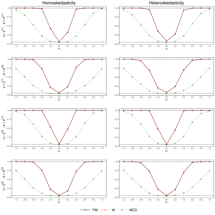
Figure C5: Power of tests with $(n,p_{x},p_{z})=(300,250,10)$ under 5% level over 1000 simulations. “MCD” represents the modified Craig–Donald test by Kolesár, (2018). The nominal size 0.05 and power 1 are shown by the horizontal dashed lines.

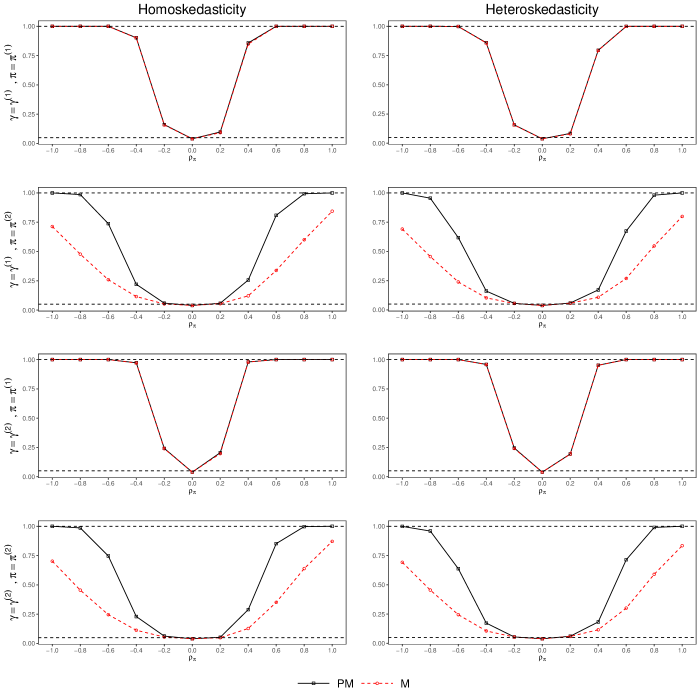
Figure C6: Power of tests with $(n,p_{x},p_{z})=(300,250,100)$ under 5% level over 1000 simulations. “MCD” represents the modified Craig–Donald test by Kolesár, (2018). The nominal size 0.05 and power 1 are shown by the horizontal dashed lines.

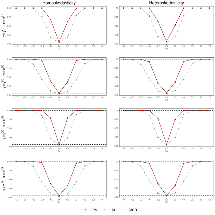
Figure C7: Power of tests with $(n,p_{x},p_{z})=(500,350,10)$ under 5% level over 1000 simulations. “MCD” represents the modified Craig–Donald test by Kolesár, (2018). The nominal size 0.05 and power 1 are shown by the horizontal dashed lines.

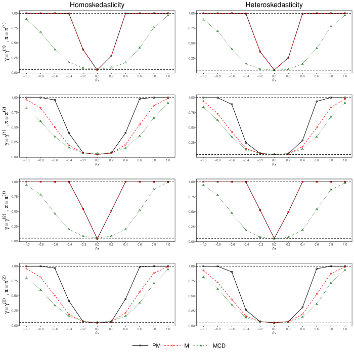
Figure C8: Power of tests with $(n,p_{x},p_{z})=(500,350,100)$ under 5% level over 1000 simulations. “MCD” represents the modified Craig–Donald test by Kolesár, (2018). The nominal size 0.05 and power 1 are shown by the horizontal dashed lines.

C.2 Simulation Results for $\beta$ Estimation

Table C1: Estimation and Inference of Endogenous Effects under Homoskedasticity

$n$	$p_{x}$	$p_{z}$	MAE			Coverage			Length
			IQ	LIML	mbtsls	IQ	LIML	mbtsls	IQ	LIML	mbtsls
$\gamma=\gamma^{(1)}$
150	50	10	0.022	0.021	0.021	0.942	0.937	0.940	0.101	0.099	0.099
		100	0.026	NA	NA	0.915	NA	NA	0.107	NA	NA
	100	10	0.023	0.029	0.029	0.935	0.945	0.947	0.106	0.139	0.142
		100	0.027	NA	NA	0.895	NA	NA	0.108	NA	NA
300	150	10	0.015	0.016	0.016	0.935	0.949	0.952	0.070	0.080	0.080
		100	0.016	0.016	0.017	0.931	0.953	0.962	0.072	0.084	0.087
	250	10	0.015	0.030	0.030	0.945	0.941	0.941	0.072	0.141	0.143
		100	0.016	NA	NA	0.929	NA	NA	0.073	NA	NA
500	350	10	0.011	0.017	0.017	0.937	0.950	0.952	0.053	0.080	0.081
		100	0.012	0.018	0.018	0.935	0.941	0.944	0.053	0.084	0.087
	450	10	0.012	0.029	0.029	0.948	0.943	0.947	0.054	0.140	0.142
		100	0.011	NA	NA	0.953	NA	NA	0.054	NA	NA
$\gamma=\gamma^{(2)}$
150	50	10	0.036	0.036	0.036	0.924	0.943	0.943	0.163	0.174	0.175
		100	0.040	NA	NA	0.892	NA	NA	0.167	NA	NA
	100	10	0.036	0.052	0.053	0.931	0.943	0.947	0.168	0.248	0.255
		100	0.040	NA	NA	0.900	NA	NA	0.166	NA	NA
300	150	10	0.024	0.028	0.028	0.936	0.942	0.946	0.113	0.141	0.142
		100	0.025	0.032	0.034	0.932	0.955	0.961	0.114	0.160	0.173
	250	10	0.024	0.053	0.054	0.950	0.937	0.934	0.115	0.250	0.257
		100	0.025	NA	NA	0.933	NA	NA	0.115	NA	NA
500	350	10	0.018	0.029	0.029	0.942	0.951	0.949	0.086	0.141	0.142
		100	0.018	0.034	0.037	0.937	0.933	0.945	0.086	0.160	0.174
	450	10	0.018	0.050	0.051	0.940	0.949	0.950	0.086	0.249	0.255
		100	0.018	NA	NA	0.957	NA	NA	0.086	NA	NA

Note: “MAE” denotes the mean absolute error. “Coverage” and “Length” are the empirical coverage rate and the average length of the 95% confidence intervals, respectively. “IQ” represents the IQ estimator defined in (5). “LIML” and “mbtsls” represent the LIML estimator and modified bias-corrected two stage least square estimator (Kolesár et al.,, 2015), respectively. The standard errors of the latter two estimators are constructed by the minimum distance approach (Kolesár,, 2018). “NA” means “not available”.

Table C2: Estimation and Inference of Endogenous Effects under Heteroskedasticity

$n$	$p_{x}$	$p_{z}$	MAE			Coverage			Length
			IQ	LIML	mbtsls	IQ	LIML	mbtsls	IQ	LIML	mbtsls
$\gamma=\gamma^{(1)}$
150	50	10	0.025	0.021	0.021	0.942	0.921	0.927	0.117	0.099	0.100
		100	0.029	NA	NA	0.918	NA	NA	0.119	NA	NA
	100	10	0.026	0.031	0.031	0.927	0.933	0.930	0.120	0.142	0.143
		100	0.029	NA	NA	0.918	NA	NA	0.122	NA	NA
300	150	10	0.017	0.017	0.017	0.935	0.929	0.928	0.081	0.080	0.080
		100	0.019	0.018	0.018	0.921	0.933	0.932	0.082	0.084	0.087
	250	10	0.019	0.029	0.030	0.932	0.943	0.943	0.083	0.141	0.143
		100	0.019	NA	NA	0.931	NA	NA	0.083	NA	NA
500	350	10	0.013	0.017	0.017	0.950	0.937	0.939	0.062	0.080	0.080
		100	0.014	0.017	0.018	0.929	0.941	0.942	0.062	0.084	0.087
	450	10	0.013	0.029	0.029	0.929	0.931	0.931	0.062	0.142	0.144
		100	0.014	NA	NA	0.933	NA	NA	0.062	NA	NA
$\gamma=\gamma^{(2)}$
150	50	10	0.045	0.039	0.039	0.935	0.914	0.921	0.208	0.174	0.176
		100	0.047	NA	NA	0.902	NA	NA	0.205	NA	NA
	100	10	0.046	0.057	0.058	0.924	0.921	0.919	0.211	0.253	0.259
		100	0.046	NA	NA	0.925	NA	NA	0.208	NA	NA
300	150	10	0.031	0.032	0.032	0.933	0.912	0.912	0.146	0.140	0.140
		100	0.033	0.035	0.038	0.904	0.925	0.924	0.147	0.159	0.174
	250	10	0.033	0.052	0.053	0.931	0.948	0.946	0.149	0.250	0.256
		100	0.032	NA	NA	0.920	NA	NA	0.148	NA	NA
500	350	10	0.023	0.030	0.030	0.944	0.923	0.929	0.113	0.140	0.141
		100	0.025	0.034	0.037	0.927	0.932	0.936	0.113	0.160	0.174
	450	10	0.024	0.053	0.054	0.938	0.936	0.938	0.113	0.252	0.258
		100	0.024	NA	NA	0.937	NA	NA	0.114	NA	NA

Note: “MAE” denotes the mean absolute error. “Coverage” and “Length” are the empirical coverage rate and the average length of the 95% confidence intervals, respectively. “IQ” represents the IQ estimator defined in (5). “LIML” and “mbtsls” represent the LIML estimator and modified bias-corrected two stage least square estimator (Kolesár et al.,, 2015), respectively. The standard errors of the latter two estimators are constructed by the minimum distance approach (Kolesár,, 2018). “NA” means “not available”.

References

- Anatolyev and Gospodinov, (2011) Anatolyev, S. and Gospodinov, N. (2011). Specification testing in models with many instruments. Econometric Theory, 27(2):427–441.
- Andrews et al., (2019) Andrews, I., Stock, J., and Sun, L. (2019). Weak instruments in IV regression: Theory and practice. Annual Review of Economics, 11:727–753.
- Angrist et al., (1999) Angrist, J. D., Imbens, G. W., and Krueger, A. B. (1999). Jackknife instrumental variables estimation. Journal of Applied Econometrics, 14(1):57–67.
- Arias-Castro et al., (2011) Arias-Castro, E., Candès, E. J., and Plan, Y. (2011). Global testing under sparse alternatives: Anova, multiple comparisons and the higher criticism. The Annals of Statistics, 39(5):2533–2556.
- Arnold et al., (2022) Arnold, D., Dobbie, W., and Hull, P. (2022). Measuring racial discrimination in bail decisions. American Economic Review, 112(9):2992–3038.
- Bai and Ng, (2010) Bai, J. and Ng, S. (2010). Instrumental variable estimation in a data rich environment. Econometric Theory, 26:1577–1606.
- Bekker and Crudu, (2015) Bekker, P. A. and Crudu, F. (2015). Jackknife instrumental variable estimation with heteroskedasticity. Journal of Econometrics, 185(2):332–342.
- Belloni et al., (2012) Belloni, A., Chen, D., Chernozhukov, V., and Hansen, C. (2012). Sparse models and methods for optimal instruments with an application to eminent domain. Econometrica, 80:2369–2429.
- Belloni et al., (2014) Belloni, A., Chernozhukov, V., and Hansen, C. (2014). Inference on treatment effects after selection among high-dimensional controls. The Review of Economic Studies, 81(2):608–650.
- Bickel et al., (2009) Bickel, P. J., Ritov, Y., and Tsybakov, A. B. (2009). Simultaneous analysis of lasso and dantzig selector. The Annals of Statistics, 37(4):1705–1732.
- Breunig et al., (2020) Breunig, C., Mammen, E., and Simoni, A. (2020). Ill-posed estimation in high-dimensional models with instrumental variables. Journal of Econometrics, 219(1):171–200.
- Bühlmann and van de Geer, (2011) Bühlmann, P. and van de Geer, S. (2011). Statistics for high-dimensional data: methods, theory and applications. Springer Science & Business Media.
- Cai and Guo, (2020) Cai, T. T. and Guo, Z. (2020). Semisupervised inference for explained variance in high dimensional linear regression and its applications. Journal of the Royal Statistical Society: Series B (Statistical Methodology), 82(2):391–419.
- Cai et al., (2011) Cai, T. T., Liu, W., and Luo, X. (2011). A constrained minimization approach to sparse precision matrix estimation. Journal of the American Statistical Association, 106(494):594–607.
- Cai et al., (2014) Cai, T. T., Liu, W., and Xia, Y. (2014). Two-sample test of high dimensional means under dependence. Journal of the Royal Statistical Society: Series B (Statistical Methodology), 76(2):349–372.
- Caner et al., (2018) Caner, M., Han, X., and Lee, Y. (2018). Adaptive elastic net GMM estimation with many invalid moment conditions: Simultaneous model and moment selection. Journal of Business & Economic Statistics, 36(1):24–46.
- Carrasco, (2012) Carrasco, M. (2012). A regularization approach to the many instruments problem. Journal of Econometrics, 170:383–398.
- Carrasco and Doukali, (2017) Carrasco, M. and Doukali, M. (2017). Efficient estimation using regularized jackknife IV estimator. Annals of Economics and Statistics, (128):109–149.
- Carrasco and Doukali, (2021) Carrasco, M. and Doukali, M. (2021). Testing overidentifying restrictions with many instruments and heteroskedasticity using regularized jackknife IV. The Econometrics Journal, pages 1–27.
- (20) Chang, J., Chen, S., Tang, C. Y., and Wu, T. T. (2021a). High-dimensional empirical likelihood inference. Biometrika, 108:127–147.
- (21) Chang, J., Shi, Z., and Zhang, J. (2021b). Culling the herd of moments with penalized empirical likelihood. arXiv preprint arXiv:2108.03382.
- Chao et al., (2014) Chao, J. C., Hausman, J. A., Newey, W. K., Swanson, N. R., and Woutersen, T. (2014). Testing overidentifying restrictions with many instruments and heteroskedasticity. Journal of Econometrics, 178:15–21.
- Cheng and Liao, (2015) Cheng, X. and Liao, Z. (2015). Select the valid and relevant moments: An information-based lasso for GMM with many moments. Journal of Econometrics, 186(2):443–464.
- Chernozhukov et al., (2013) Chernozhukov, V., Chetverikov, D., and Kato, K. (2013). Gaussian approximations and multiplier bootstrap for maxima of sums of high-dimensional random vectors. The Annals of Statistics, 41(6):2786–2819.
- Chernozhukov et al., (2015) Chernozhukov, V., Hansen, C., and Spindler, M. (2015). Post-selection and post-regularization inference in linear models with many controls and instruments. American Economic Review, 105(5):486–90.
- Donald and Newey, (2001) Donald, S. and Newey, W. (2001). Choosing the number of instruments. Econometrica, 69:1161–1191.
- Donald et al., (2003) Donald, S. G., Imbens, G. W., and Newey, W. K. (2003). Empirical likelihood estimation and consistent tests with conditional moment restrictions. Journal of Econometrics, 117(1):55–93.
- Donoho and Jin, (2004) Donoho, D. and Jin, J. (2004). Higher criticism for detecting sparse heterogeneous mixtures. The Annals of Statistics, 32(3):962–994.
- Fan et al., (2015) Fan, J., Liao, Y., and Yao, J. (2015). Power enhancement in high-dimensional cross-sectional tests. Econometrica, 83(4):1497–1541.
- Fan et al., (2021) Fan, J., Weng, H., and Zhou, Y. (2021). Optimal estimation of functionals of high-dimensional mean and covariance matrix. arXiv preprint arXiv:1908.07460.
- Fan and Wu, (2022) Fan, Q. and Wu, Y. (2022). Endogenous treatment effect estimation with a large and mixed set of instruments and control variables. The Review of Economics and Statistics, pages 1–45.
- Fan and Zhong, (2018) Fan, Q. and Zhong, W. (2018). Nonparametric additive instrumental variable estimator: A group shrinkage estimation perspective. Journal of Business & Economic Statistics, 36(3):388–399.
- Frandsen et al., (2023) Frandsen, B., Lefgren, L., and Leslie, E. (2023). Judging judge fixed effects. American Economic Review, 113(1):253–277.
- Frankel and Romer, (1999) Frankel, J. A. and Romer, D. H. (1999). Does trade cause growth? American Economic Review, 89(3):379–399.
- Gold et al., (2020) Gold, D., Lederer, J., and Tao, J. (2020). Inference for high-dimensional instrumental variables regression. Journal of Econometrics, 217(1):79–111.
- Guo, (2021) Guo, Z. (2021). Post-selection problems for causal inference with invalid instruments: A solution using searching and sampling. arXiv e-prints, pages arXiv–2104.
- (37) Guo, Z., Kang, H., Cai, T. T., and Small, D. S. (2018a). Confidence intervals for causal effects with invalid instruments by using two-stage hard thresholding with voting. Journal of the Royal Statistical Society: Series B (Statistical Methodology), 80(4):793–815.
- (38) Guo, Z., Kang, H., Cai, T. T., and Small, D. S. (2018b). Testing endogeneity with high dimensional covariates. Journal of Econometrics, 207(1):175–187.
- Guo et al., (2021) Guo, Z., Renaux, C., Bühlmann, P., and Cai, T. T. (2021). Group inference in high dimensions with applications to hierarchical testing. Electronic Journal of Statistics, 15(2):6633–6676.
- Guo et al., (2019) Guo, Z., Wang, W., Cai, T. T., and Li, H. (2019). Optimal estimation of genetic relatedness in high-dimensional linear models. Journal of the American Statistical Association, 114(525):358–369.
- Hall and Heyde, (1980) Hall, P. and Heyde, C. C. (1980). Martingale limit theory and its application. Academic Press.
- Hansen and Kozbur, (2014) Hansen, C. and Kozbur, D. (2014). Instrumental variables estimation with many weak instruments using regularized jive. Journal of Econometrics, 182(2):290–308.
- Hansen, (1982) Hansen, L. P. (1982). Large sample properties of generalized method of moments estimators. Econometrica, pages 1029–1054.
- Ingster and Suslina, (2003) Ingster, Y. and Suslina, I. (2003). Nonparametric Goodness-of-fit Testing under Gaussian Models. Springer.
- Javanmard and Montanari, (2014) Javanmard, A. and Montanari, A. (2014). Confidence intervals and hypothesis testing for high-dimensional regression. The Journal of Machine Learning Research, 15(1):2869–2909.
- Kang et al., (2016) Kang, H., Zhang, A., Cai, T. T., and Small, D. S. (2016). Instrumental variables estimation with some invalid instruments and its application to mendelian randomization. Journal of the American Statistical Association, 111(513):132–144.
- Kock and Preinerstorfer, (2019) Kock, A. B. and Preinerstorfer, D. (2019). Power in high-dimensional testing problems. Econometrica, 87(3):1055–1069.
- Kock and Preinerstorfer, (2021) Kock, A. B. and Preinerstorfer, D. (2021). Consistency of -norm based tests in high dimensions: characterization, monotonicity, domination. arXiv preprint arXiv:2103.11201.
- Kolesár, (2018) Kolesár, M. (2018). Minimum distance approach to inference with many instruments. Journal of Econometrics, 204(1):86–100.
- Kolesár et al., (2015) Kolesár, M., Chetty, R., Friedman, J., Glaeser, E., and Imbens, G. W. (2015). Identification and inference with many invalid instruments. Journal of Business & Economic Statistics, 33(4):474–484.
- Lee and Okui, (2012) Lee, Y. and Okui, R. (2012). Hahn–Hausman test as a specification test. Journal of Econometrics, 167(1):133–139.
- Liang et al., (2022) Liang, X., Sanderson, E., and Windmeijer, F. (2022). Selecting valid instrumental variables in linear models with multiple exposure variables: Adaptive lasso and the median-of-medians estimator. arXiv preprint arXiv:2208.05278.
- Liao, (2013) Liao, Z. (2013). Adaptive GMM shrinkage estimation with consistent moment selection. Econometric Theory, 29(5):857–904.
- Mei and Shi, (2022) Mei, Z. and Shi, Z. (2022). On lasso for high dimensional predictive regression. arXiv preprint arXiv:2212.07052.
- Merlevède et al., (2011) Merlevède, F., Peligrad, M., and Rio, E. (2011). A Bernstein type inequality and moderate deviations for weakly dependent sequences. Probability Theory and Related Fields, 151(3):435–474.
- Mikusheva and Sun, (2020) Mikusheva, A. and Sun, L. (2020). Inference with many weak instruments. arXiv preprint arXiv:2004.12445.
- Okui, (2011) Okui, R. (2011). Instrumental variable estimation in the presence of many moment conditions. Journal of Econometrics, 165:70–86.
- Pang et al., (2014) Pang, H., Liu, H., and Vanderbei, R. J. (2014). The fastclime package for linear programming and large-scale precision matrix estimation in R. Journal of Machine Learning Research.
- Sargan, (1958) Sargan, J. D. (1958). The estimation of economic relationships using instrumental variables. Econometrica, pages 393–415.
- Sun et al., (2021) Sun, B., Liu, Z., and Tchetgen Tchetgen, E. (2021). On multiply robust mendelian randomization (mr2) with many invalid genetic instruments. medRxiv.
- Tibshirani, (1996) Tibshirani, R. (1996). Regression shrinkage and selection via the lasso. Journal of the Royal Statistical Society: Series B (Methodological), 58(1):267–288.
- van de Geer et al., (2014) van de Geer, S., Bühlmann, P., Ritov, Y., and Dezeure, R. (2014). On asymptotically optimal confidence regions and tests for high-dimensional models. The Annals of Statistics, 42(3):1166–1202.
- Vershynin, (2010) Vershynin, R. (2010). Introduction to the non-asymptotic analysis of random matrices. arXiv preprint arXiv:1011.3027.
- Windmeijer et al., (2019) Windmeijer, F., Farbmacher, H., Davies, N., and Davey Smith, G. (2019). On the use of the lasso for instrumental variables estimation with some invalid instruments. Journal of the American Statistical Association, 114(527):1339–1350.
- Windmeijer et al., (2021) Windmeijer, F., Liang, X., Hartwig, F. P., and Bowden, J. (2021). The confidence interval method for selecting valid instrumental variables. Journal of the Royal Statistical Society: Series B (Statistical Methodology), 83(4):752–776.
- Ye et al., (2021) Ye, T., Liu, Z., Sun, B., and Tchetgen Tchetgen, E. (2021). GENIUS-MAWII: For robust mendelian randomization with many weak invalid instruments. arXiv preprint arXiv:2107.06238.
- Zhang and Zhang, (2014) Zhang, C.-H. and Zhang, S. (2014). Confidence intervals for low dimensional parameters in high dimensional linear models. Journal of the Royal Statistical Society: Series B (Statistical Methodology), 76(1):217–242.
- Zhang and Cheng, (2017) Zhang, X. and Cheng, G. (2017). Simultaneous inference for high-dimensional linear models. Journal of the American Statistical Association, 112(518):757–768.
- Zhu, (2018) Zhu, Y. (2018). Sparse linear models and -regularized 2SLS with high-dimensional endogenous regressors and instruments. Journal of Econometrics, 202(2):196–213.