Deep Ensemble as a Gaussian Process Approximate Posterior

Abstract

Deep Ensemble (DE) is an effective alternative to Bayesian neural networks for uncertainty quantification in deep learning. The uncertainty of DE is usually conveyed by the functional inconsistency among the ensemble members, say, the disagreement among their predictions. Yet, the functional inconsistency stems from unmanageable randomness and may easily collapse in specific cases. To render the uncertainty of DE reliable, we propose a refinement of DE where the functional inconsistency is explicitly characterized, and further tuned w.r.t. the training data and certain priori beliefs. Specifically, we describe the functional inconsistency with the empirical covariance of the functions dictated by ensemble members, which, along with the mean, define a Gaussian process (GP). Then, with specific priori uncertainty imposed, we maximize functional evidence lower bound to make the GP specified by DE approximate the Bayesian posterior. In this way, we relate DE to Bayesian inference to enjoy reliable Bayesian uncertainty. Moreover, we provide strategies to make the training efficient. Our approach consumes only marginally added training cost than the standard DE, but achieves better uncertainty quantification than DE and its variants across diverse scenarios.

[#1]

1 Introduction

Bayesian treatment of deep neural networks (DNNs) is promised to enjoy principled Bayesian uncertainty while unleashing the capacity of DNNs, with Bayesian neural networks (BNNs) as popular examples (MacKay, 1992; Hinton & Van Camp, 1993; Neal, 1995; Graves, 2011). Nevertheless, despite the surge of advance in BNNs (Louizos & Welling, 2016; Zhang et al., 2018), many existing BNNs still face obstacles in accurate and scalable inference (Sun et al., 2019), and exhibit limitations in uncertainty quantification and out-of-distribution robustness (Ovadia et al., 2019).

Alternatively, Deep Ensemble (DE) (Lakshminarayanan et al., 2017) trains multiple independent, randomly-initialized DNNs for ensemble, presenting higher flexibility and effectiveness than BNNs. Practitioners tend to interpret the functional inconsistency among the ensemble members, say, the disagreement among their predictions, as a proxy of DE’s uncertainty. However, the functional inconsistency stems from the unmanageable randomness in DNN initialization and stochastic gradient descent (SGD), thus is likely to collapse in specific cases (see Figure 2). To fix this issue, recent works like RMS (Lu & Van Roy, 2017; Osband et al., 2018; Pearce et al., 2020) and NTKGP (He et al., 2020) refine DE to be a Bayesian inference approach in the spirit of “sample-then-optimize” (Matthews et al., 2017). Yet, these works often make strong assumptions like Gaussian likelihoods and linearized/infinite-width models.

This work aims at tackling these issues. We first reveal that the unreliable uncertainty of DE arises from the gap that the functional inconsistency are not properly adapted w.r.t. the training data and certain priori beliefs, but is leveraged to quantify post data uncertainty in the test phase. To bridge the gap, we propose to explicitly incorporate the functional inconsistency into modeling. Viewing the ensemble members as a set of basis functions, the functional inconsistency can be formally described by their empirical covariance, which, along with their mean, specify a Gaussian process (GP). Such a GP is referred to as DE-GP for short hereinafter. Given this setup, we advocate tuning the whole DE-GP, including its mean and covariance, w.r.t. the training data under the functional variational inference (fVI) paradigm (Sun et al., 2019) given specific priors. Namely, we regard DE-GP as an parametric approximate posterior so as to enjoy the principled Bayesian uncertainty. By fVI, DE-GP can handle classification problems directly and exactly, without casting them into regression ones as done by some existing Bayesian variants of DE (He et al., 2020).

Without loss of generality, we adopt a prior also in the form of GP, then the gradients of the KL divergence between the DE-GP approximate posterior and the GP prior involved in fVI can be easily estimated without reliance on complicated gradient estimators (Shi et al., 2018b). We provide recipes to make the training even faster, then the additional computation overhead induced by DE-GP upon DE is minimal. We also identify the necessity of including an extra weight-space regularization term to guarantee the generalization performance of DE-GP when using deep architectures.

Empirically, DE-GP outperforms DE and its variants on various regression datasets, and presents superior uncertainty estimates and out-of-distribution robustness without compromising accuracy in standard image classification tasks. DE-GP also shows promise in solving contextual bandit problems, where the uncertainty guides exploration.

2 Related Work

Bayesian neural networks. Bayesian treatment of DNNs is an emerging topic yet with a long history (Mackay, 1992; Hinton & Van Camp, 1993; Neal, 1995; Graves, 2011). BNNs can be learned by variational inference (Blundell et al., 2015; Hernández-Lobato & Adams, 2015; Louizos & Welling, 2016; Zhang et al., 2018; Khan et al., 2018; Deng et al., 2020), Laplace approximation (Mackay, 1992; Ritter et al., 2018), Markov chain Monte Carlo (Welling & Teh, 2011; Chen et al., 2014; Zhang et al., 2019), particle-optimization based variational inference (Liu & Wang, 2016), Monte Carlo dropout (Gal & Ghahramani, 2016), and other methods (Maddox et al., 2019). To avoid the difficulties of posterior inference in weight space, some recent works advocate performing Bayesian inference in function space (Sun et al., 2019; Rudner et al., 2021; Wang et al., 2019). In function space, BNNs of infinite or even finite width equal to GPs (Neal, 1996; Lee et al., 2018; Novak et al., 2018; Khan et al., 2019), which provides supports for constructing an approximate posterior in the form of GP.

Deep Ensemble. As an alternative to BNNs, DE (Lakshminarayanan et al., 2017) has shown promise in diverse uncertainty quantification scenarios (Ovadia et al., 2019), yet lacks a proper Bayesian interpretation. Wilson & Izmailov (2020) interpreted DE as a method that approximates the Bayesian posterior predictive, but it is hard to judge whether the approximation is reliable or not in practice. The notion of “sample-then-optimize” (Matthews et al., 2017) has also been considered to make DE Bayesian. For example, RMS (Lu & Van Roy, 2017; Osband et al., 2018; Pearce et al., 2020) regularizes the ensemble members towards randomised priors to obtain posterior samples, while it typically assumes linear data likelihood which is impractical for deep models and classification tasks. He et al. (2020) proposed to add a randomised function to each ensemble member to realize a function-space Bayesian interpretation, but the method is asymptotically exact in the infinite width limit and is limited to regressions. By contrast, DE-GP works without restrictive assumptions. In parallel, D’Angelo & Fortuin (2021) proposed to add a repulsive term to DE but the method relies on less scalable gradient estimators.

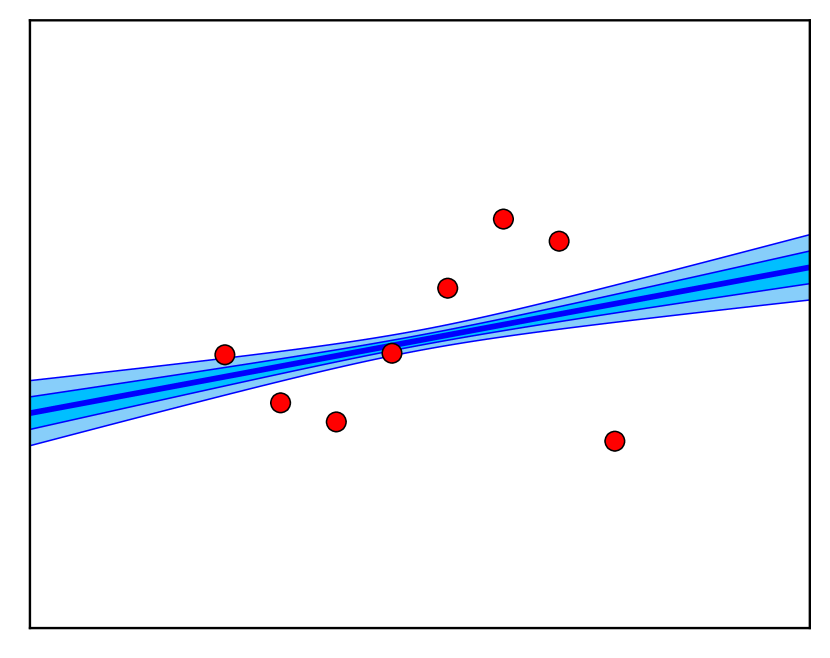
0 hidden layer

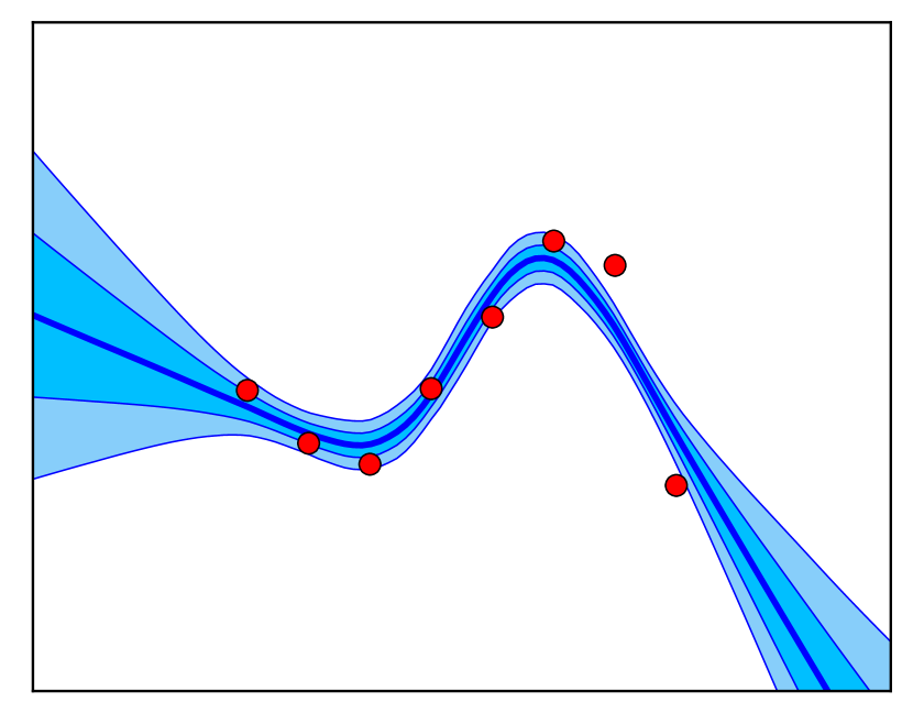
1 hidden layer

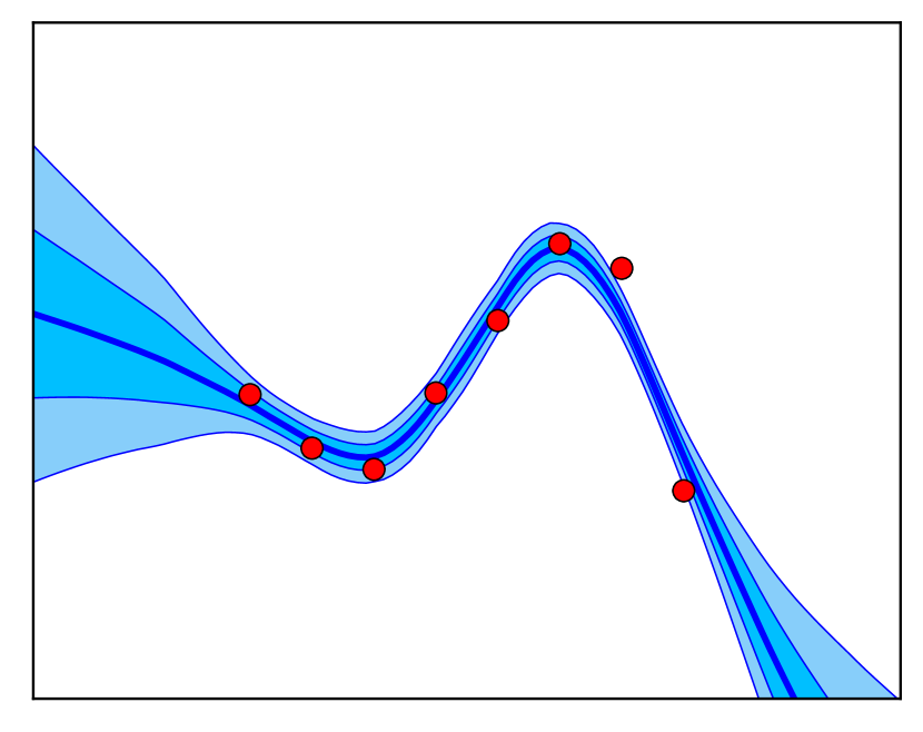
2 hidden layers

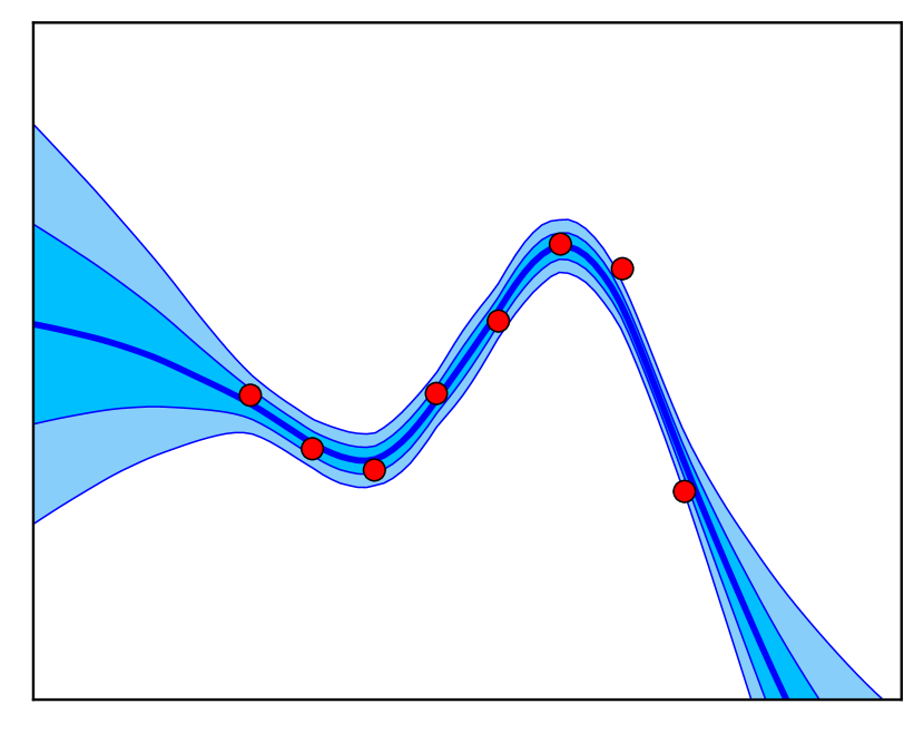
3 hidden layers

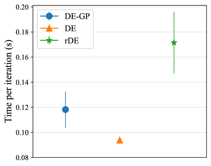
Training speed comparison

Figure 1: DE-GP behaves similarly to the non-parameteric NN-GP (the gold standard), with only marginally added overheads upon DE. The settings are identical to those in Figure 2. The training speed is measured with the MLP architecture with 3 hidden layers of size 256.

DE

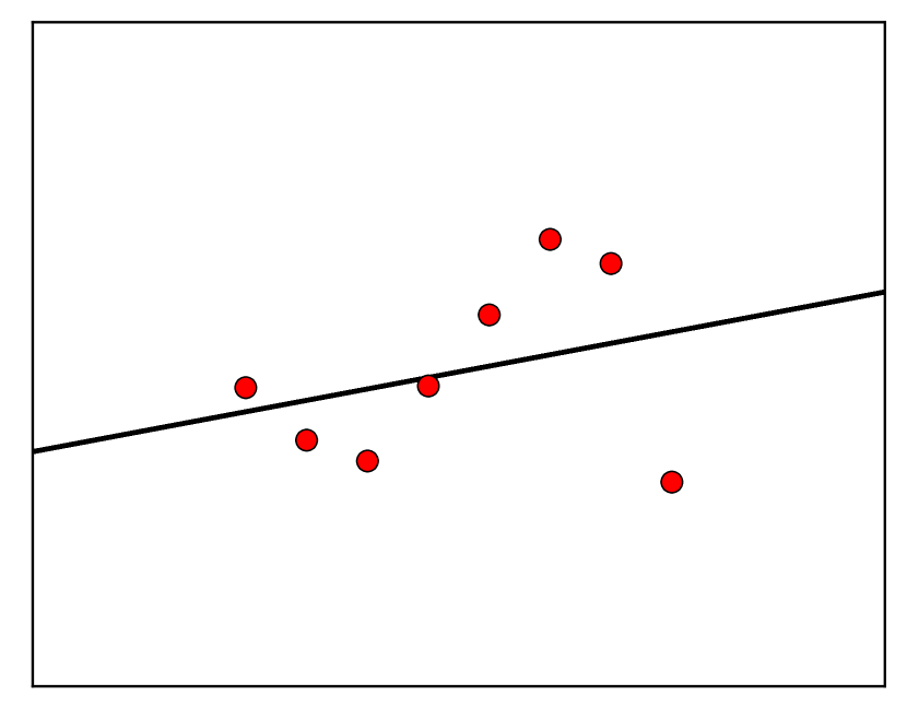
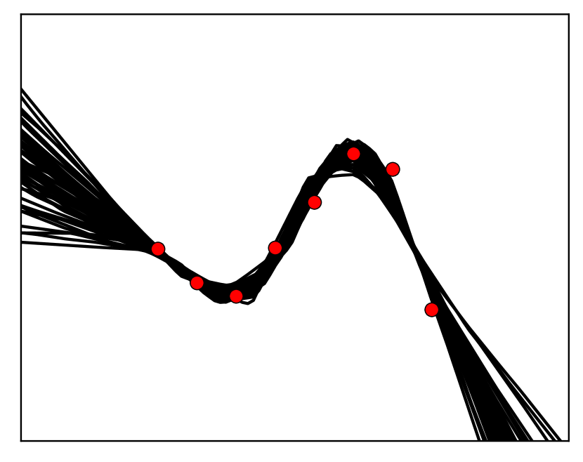
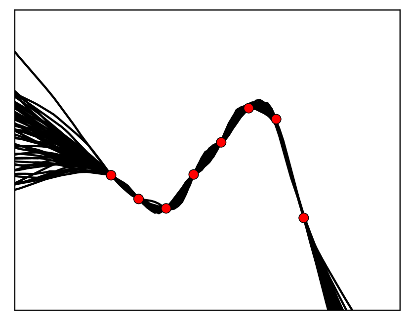
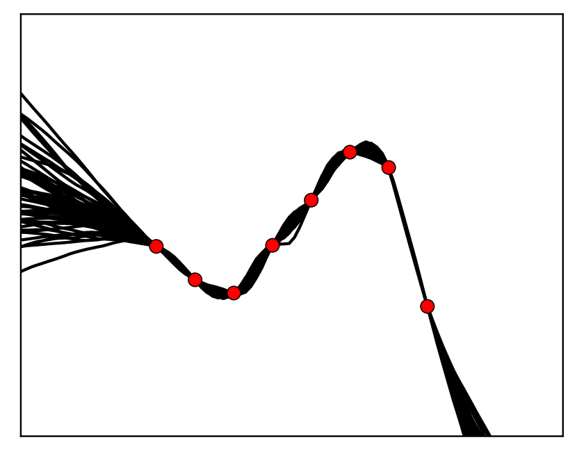
rDE

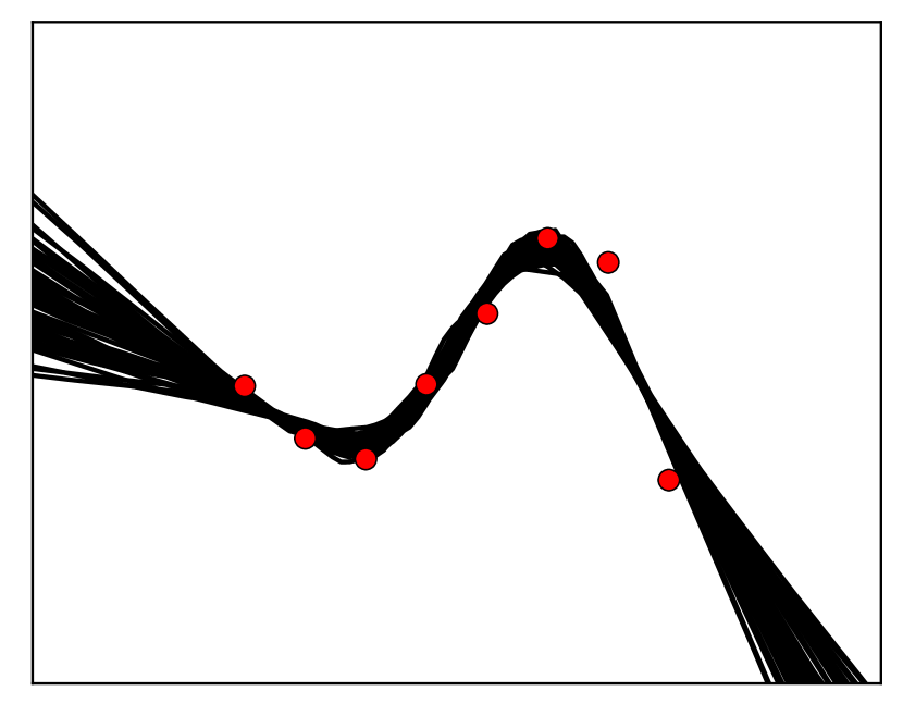
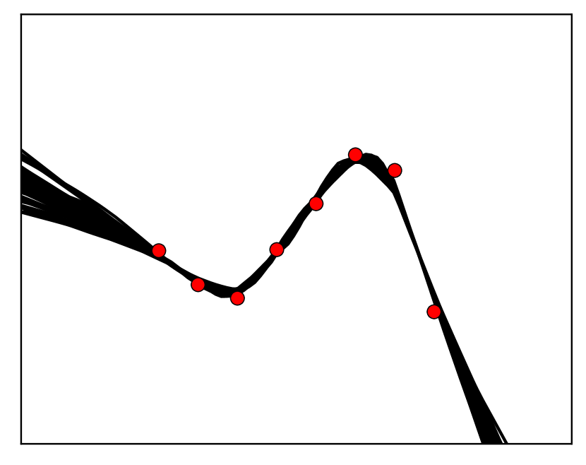
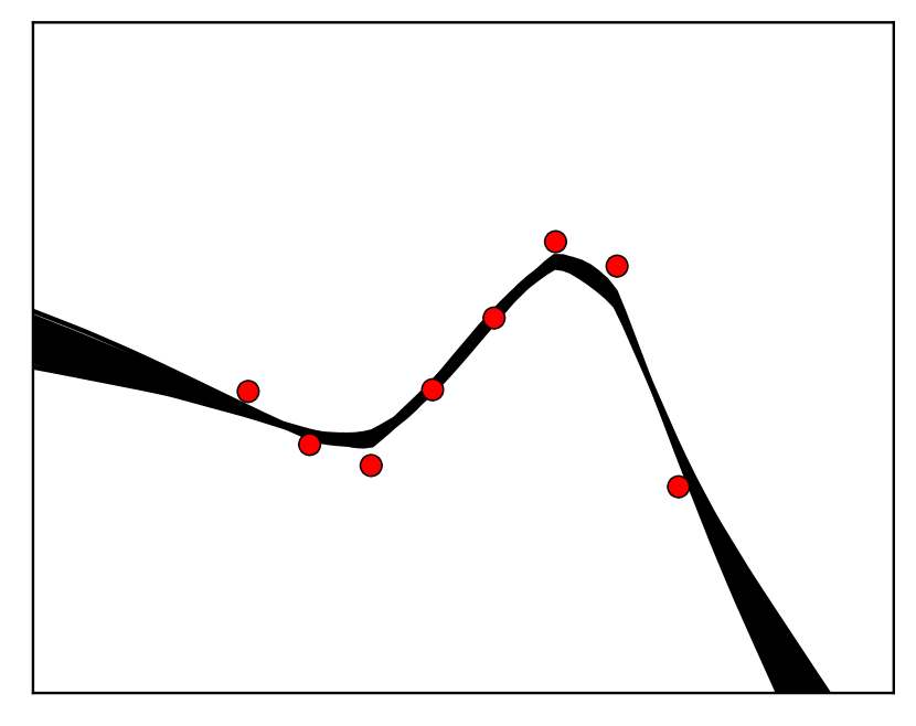
NN-GP

0 hidden layer

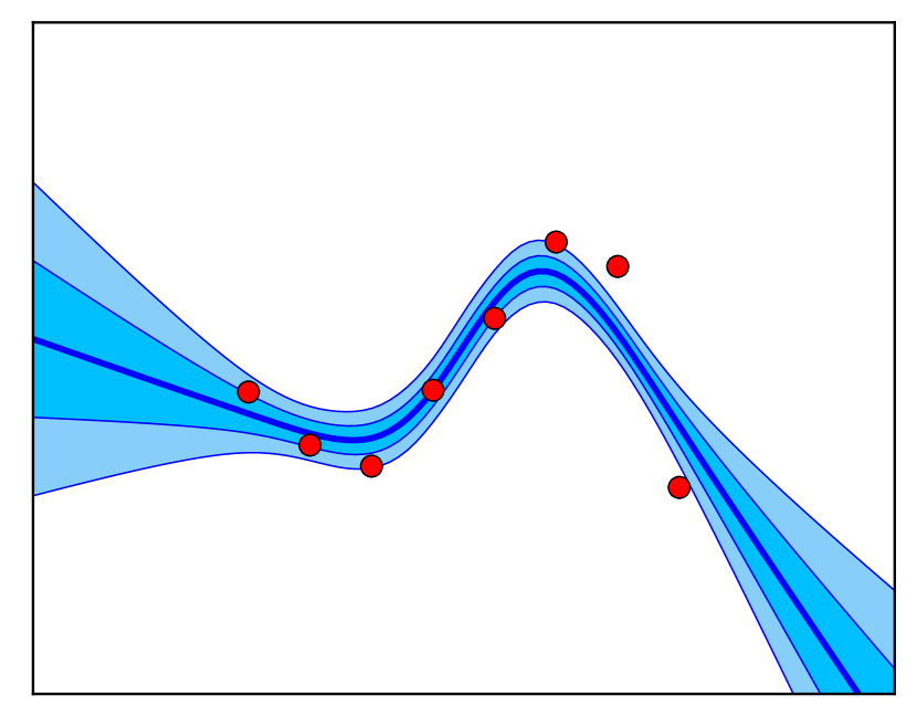
1 hidden layer

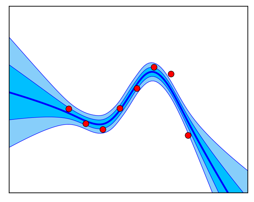
2 hidden layers

3 hidden layers

Figure 2: 1-D regression on $y=\sin 2x+\epsilon,\epsilon\sim\mathcal{N}(0,0.2)$. Red dots refer to the training data (the rightest dot is deliberately perturbed to cause significant data noise). Rows: DE, rDE and NN-GP (the gold standard). Columns: using multilayer perceptrons (MLPs) architectures with 0 hidden layer, 1 hidden layer of size 64, 2 hidden layers of size 128, and 3 hidden layers of size 256. DE and rDE use $50$ MLPs for ensemble. The weight-space priors for rDE and NN-GP are Gaussian distributions. Black lines for DE and rDE refer to the predictions of the ensemble members. Dark blue curves and shaded regions for DE-GP refer to mean predictions and uncertainty. Compared to NN-GP, DE and rDE suffer from over-confidence and less calibrated uncertainty estimates.

3 Motivation

Assuming access to a dataset $\mathcal{D}=(\mathbf{X},\mathbf{Y})=\{({\bm{x}}_{i},{\bm{y}}_{i})\}_{i=1}^{n}$, with ${\bm{x}}_{i}\in\mathcal{X}$ as data and ${\bm{y}}_{i}$ as $C$-dimensional targets, we can use a DNN $g(\cdot,{\bm{w}}):\mathcal{X}\rightarrow\mathbb{R}^{C}$ with weights ${\bm{w}}$ to fit it. Despite impressive performance, the regularly trained DNNs are prone to over-confidence, making it hard to decide how certain they are about the predictions. Lacking the ability to reliably quantify predictive uncertainty is unacceptable for realistic decision-making scenarios.

A principled mechanism for uncertainty quantification in deep learning is to apply Bayesian treatment to DNNs to reason about Bayesian uncertainty. The resulting models are known as BNNs. In BNNs, ${\bm{w}}$ is treated as a random variable. Given some prior beliefs $p({\bm{w}})$, we chase the posterior $p({\bm{w}}|\mathcal{D})$. In practice, it is intractable to analytically compute the true posterior $p({\bm{w}}|\mathcal{D})$ due to the high non-linearity of DNNs, so some approximate posterior $q({\bm{w}})$ is usually found by techniques like variational inference (Blundell et al., 2015), Laplace approximation (Mackay, 1992), Monte Carlo dropout (Gal & Ghahramani, 2016), etc.

BNNs marginalize over the posterior to predict for new data ${\bm{x}}^{*}$ (a.k.a. the posterior predictive):

$$p(y|{\bm{x}}^{*},\mathcal{D}) =\mathbb{E}_{p({\bm{w}}|\mathcal{D})}p(y|{\bm{x}}^{*},{\bm{w}})$$ (1)

$$\approx\mathbb{E}_{q({\bm{w}})}p(y|{\bm{x}}^{*},{\bm{w}})\approx\frac{1}{S}\sum_{s=1}^{S}p(y|{\bm{x}}^{*},{\bm{w}}_{s}),$$

where ${\bm{w}}_{s}\sim q({\bm{w}}),s=1,...,S$. This procedure propagates the embedded model uncertainty into the prediction. However, most of the existing BNN approaches face obstacles in precise posterior inference due to non-trivial and convoluted posterior dependencies (Louizos & Welling, 2016; Zhang et al., 2018; Shi et al., 2018a; Sun et al., 2019), and deliver unsatisfactory uncertainty estimates and out-of-distribution (OOD) robustness (Ovadia et al., 2019).

As a workaround of BNNs, Deep Ensemble (DE) (Lakshminarayanan et al., 2017) deploys a set of $M$ DNNs $\{g(\cdot,{\bm{w}}_{i})\}_{i=1}^{M}$ to interpret the data from different angles. In this sense, we can view DE as an approximate posterior in the form of a mixture of deltas (MoD) $q({\bm{w}})=\frac{1}{M}\sum_{i=1}^{M}\delta({\bm{w}}-{\bm{w}}_{i})$. Nevertheless, instead of being tuned under Bayesian inference principles, the ensemble members are independently trained under deterministic learning principles like maximum likelihood estimation (MLE) and maximum a posteriori (MAP) (we refer to the resulting models as DE and regularized DE (rDE) respectively):

$$\max_{{\bm{w}}_{1},...,{\bm{w}}_{M}}\mathcal{L}_{\text{DE}}= \max_{{\bm{w}}_{1},...,{\bm{w}}_{M}}\frac{1}{M}\sum_{i=1}^{M}\log p(\mathcal{D}|{\bm{w}}_{i}),$$ (2)

$$\max_{{\bm{w}}_{1},...,{\bm{w}}_{M}}\mathcal{L}_{\text{rDE}}= \max_{{\bm{w}}_{1},...,{\bm{w}}_{M}}\frac{1}{M}\sum_{i=1}^{M}[\log p(\mathcal{D}|{\bm{w}}_{i})+\log p({\bm{w}}_{i})].$$

The randomness in initialization and SGD diversifies the ensemble members, making them explore distinct modes of the non-convex loss landscape of DNNs (Fort et al., 2019; Wilson & Izmailov, 2020), and in turn boost the ensemble performance. In parallel, researchers have found that DE is also promising in quantifying uncertainty (Lakshminarayanan et al., 2017; Ovadia et al., 2019). The functional inconsistency among the ensemble members is usually interpreted as a proxy of DE’s uncertainty. However, we question the efficacy of the uncertainty of DE given that the functional inconsistency arises from the randomness in DNN initialization and SGD instead of a Bayesian treatment, i.e., the true model uncertainty is not explicitly considered during training. To confirm this apprehension, we evaluate DE and rDE on a simple 1-D regression problem. We choose neural network Gaussian process (NN-GPs) (Neal, 1996) as a golden standard because it equals to BNNs in the infinite-width limit and allows for analytical function-space posterior inference. We depict the results in Figure 2.

The results echo our concerns on DE. It is evident that (i) DE and rDE collapse to a single model in the linear case (the first column), attributed to that the loss surface is convex w.r.t. the model parameters; (ii) DE and rDE reveal minimal uncertainty in in-distribution regions, although there is severe data noise; (iii) the uncertainty of DE and rDE deteriorates as the model size increases regardless of whether there is over-fitting.

In essence, the functional inconsistency in DE has not been properly adapted w.r.t. the priori uncertainty and training data, but is used to quantify post data uncertainty. Such a gap is thought of as the cause of the unreliability issue of DE’s uncertainty. Having identified this, we propose to incorporate the functional inconsistency into modeling, and perform Bayesian inference to tune the whole model to enjoy principled Bayesian uncertainty. We describe how to realize this in the following.

4 Methodology

This section provides the details for the modeling, inference, and training procedure of the proposed DE-GP. We impress the readers in advance by the results of DE-GP on the aforementioned regression problem shown in Figure 1.

4.1 Modeling

Viewing the ensemble members $\{g(\cdot,{\bm{w}}_{i})\}_{i=1}^{M}$ as a set of basis functions, the functional inconsistency among them can be formally represented by the empirical covariance of these functions in the following form:

$$\small\scalebox{1.0}{$k({\bm{x}},{\bm{x}}^{\prime}):=\frac{1}{M}\sum_{i=1}^{M}\left(g_{i}({\bm{x}})-m({\bm{x}})\right)\left(g_{i}({\bm{x}}^{\prime})-m({\bm{x}}^{\prime})\right)^{\top}$},$$ (3)

where $g_{i}$ refers to $g(\cdot,{\bm{w}}_{i})$ and $m({\bm{x}}):=\frac{1}{M}\sum_{i=1}^{M}g_{i}({\bm{x}})$. From the definition, $k$ is a matrix-valued kernel, with values in the space of $C\times C$ matrices.

Then, the incorporation of functional inconsistency amounts to building a model with $k({\bm{x}},{\bm{x}}^{\prime})$. Naturally, the DE-GP $\mathcal{GP}(f|m({\bm{x}}),k({\bm{x}},{\bm{x}}^{\prime}))$ comes into the picture. Nevertheless, $k({\bm{x}},{\bm{x}}^{\prime})$ is of low rank, so we opt to add a small scaled identity matrix $\lambda\mathbf{I}_{C}$ upon $k({\bm{x}},{\bm{x}}^{\prime})$ to avoid singularity. Unless specified otherwise, we refer to the resulting covariance kernel as $k({\bm{x}},{\bm{x}}^{\prime})$ in the following.

We can train both DE-GP and DE to approximate the true Bayesian posteriors associated with some priors. In this sense, DE-GP shifts the family of the approximate posteriors from MoDs, which are singular and often lead to ill-defined learning objectives (Hron et al., 2018), to the amenable GPs. The variations in $k({\bm{x}},{\bm{x}}^{\prime})$ are confined to having up to $M-1$ rank, echoing the recent investigations showing that low-rank approximate posteriors for deep models conjoin effectiveness and efficiency (Maddox et al., 2019; Izmailov et al., 2020; Dusenberry et al., 2020).

Akin to the kernels in (Wilson et al., 2016), the DE-GP kernels are highly flexible, and may automatically discover the underlying structures of high-dimensional data without manual participation.

4.2 Inference

As stated above, we take DE-GP as a parametric approximate posterior, i.e., $q(f)=\mathcal{GP}(f|m({\bm{x}}),k({\bm{x}},{\bm{x}}^{\prime}))$, and push it to approach the true posterior over functions associated with specific priors by fVI (Sun et al., 2019).

Prior We can freely choose a distribution over functions (i.e., a stochastic process) as the prior attributed to the fVI paradigm. Without loss of generality, we use the MC estimates of NN-GPs (MC NN-GPs) (Novak et al., 2018) as the prior because (i) they correspond to the Gaussian priors on weights $p({\bm{w}})=\mathcal{N}(\bm{0},\texttt{diag}(\bm{\sigma_{0}^{2}}))$ ; (ii) they carry valuable inductive bias of certain finitely wide DNN architectures; (iii) they are more accessible than NN-GPs in practice; (iv) they have been evaluated in some related works like (Wang et al., 2019). Concretely, supposing a finitely wide DNN composed of a feature projector ${h(\cdot,{\bm{w}}):\mathcal{X}\rightarrow\mathbb{R}^{\hat{C}}}$ and a linear readout layer with weight variance $\sigma_{w}^{2}$ and bias variance $\sigma_{b}^{2}$, the MC NN-GP prior is $p(f)=\mathcal{GP}(f|0,k_{p}({\bm{x}},{\bm{x}}^{\prime}))$, where

$$k_{p}({\bm{x}},{\bm{x}}^{\prime}) :=(\sigma_{w}^{2}\hat{k}_{p}({\bm{x}},{\bm{x}}^{\prime})+\sigma_{b}^{2})\mathbf{I}_{C},$$ (4)

$$\text{and}\,\,\hat{k}_{p}({\bm{x}},{\bm{x}}^{\prime}) :=\frac{1}{S\hat{C}}\sum_{s=1}^{S}h({\bm{x}},{\bm{w}}_{s})^{\top}h({\bm{x}}^{\prime},{\bm{w}}_{s}).$$

${\bm{w}}_{s}$ are i.i.d. samples from $p({\bm{w}})$. We highlight that $\hat{k}_{p}$ is scalar-valued yet ${k}_{p}$ is matrix-valued. Keep in mind that the MC NN-GP priors can be defined with distinct architectures from the DE-GP approximate posteriors.

In practice, DE-GP benefits from learning in the parametric family specified by DNNs ensemble, hence can even outperform the analytical NN-GP posteriors on some metrics.

fELBO Following (Sun et al., 2019), we maximize the functional ELBO (fELBO) to achieve fVI:

$$\small\max_{q(f)}\mathbb{E}_{q(f)}[\log p(\mathcal{D}|f)]-D_{\mathrm{KL}}[q(f)\|p(f)].$$ (5)

Notably, there is a KL divergence between two GPs, which, on its own, is challenging to cope with. Fortunately, as proved by (Sun et al., 2019), we can take the KL divergence between the marginal distributions of function evaluations as a substitute for it, giving rise to a more tractable objective:

$$\scalebox{0.9}{$\mathcal{L}=\mathbb{E}_{q(f)}\left[\sum_{({\bm{x}}_{i},{\bm{y}}_{i})\in\mathcal{D}}\log p({\bm{y}}_{i}|f({\bm{x}}_{i}))\right]-D_{\mathrm{KL}}\left[q(\mathbf{f}^{\tilde{\mathbf{X}}})\|p(\mathbf{f}^{\tilde{\mathbf{X}}})\right],$}$$ (6)

where $\tilde{\mathbf{X}}$ denotes a measurement set including all training inputs $\mathbf{X}$, and $\mathbf{f}^{\tilde{\mathbf{X}}}$ is the concatenation of the vectorized outputs of $f$ for $\tilde{\mathbf{X}}$, i.e., $\mathbf{f}^{\tilde{\mathbf{X}}}\in\mathbb{R}^{|\tilde{\mathbf{X}}|C}$.

It has recently been shown that the fELBO is often ill-defined, since the KL divergence in function space is infinite (Burt et al., 2020), which may lead to several pathologies. Yet, Figure 1 and Figure 2, which form posterior approximation quality checks, prove the empirical efficacy of the used fELBO.

4.3 Training

We outline the training procedure of DE-GP in Algorithm 1, and elaborate some details below.

4.3.1 Mini-batch Training

In deep learning scenarios, DE-GP should proceed by mini-batch training. At each step, we manufacture a stochastic measurement set with a mini-batch $\mathcal{D}_{s}=(\mathbf{X}_{s},\mathbf{Y}_{s})$ from the training data $\mathcal{D}$ and some random samples $\mathbf{X}_{\nu}$ from a continuous distribution (e.g., a uniform distribution) $\nu$ supported on $\mathcal{X}$. Then, we adapt the objective defined in Equation 6 to the following form:

$$\underset{{\bm{w}}_{1},...,{\bm{w}}_{M}}{\max}\,\mathcal{L}=\underset{{\bm{w}}_{1},...,{\bm{w}}_{M}}{\max} \scalebox{0.95}{$\mathbb{E}_{f\sim q(f)}\left[\sum_{({\bm{x}}_{i},{\bm{y}}_{i})\in\mathcal{D}_{s}}\log p({\bm{y}}_{i}|f({\bm{x}}_{i}))\right]$}$$ (7)

$$\;\scalebox{0.95}{$-\,\alpha D_{\mathrm{KL}}\left[q(\mathbf{f}^{\tilde{\mathbf{X}}_{s}})\|p(\mathbf{f}^{\tilde{\mathbf{X}}_{s}})\right]$},$$

where ${\tilde{\mathbf{X}}_{s}}$ indicates the union of ${\mathbf{X}_{s}}$ and ${\mathbf{X}_{\nu}}$. We opt to fix the hyper-parameters specifying the MC NN-GP prior $p(f)$, but to tune the coefficient $\alpha$ to better trade off between data evidence and priori regularization rather than fixing $\alpha$ as 1. When tuning $\alpha$, we intentionally set it as large as possible to avoid colder posteriors and worse uncertainty estimates.

The importance of the incorporation of extra measurement points $\mathbf{X}_{\nu}$ depends on the data and the problem at hand. Section B.2 reports a study on the aforementioned 1-D regression where the DE-GP is trained without the incorporation of $\mathbf{X}_{\nu}$, and the results are still seemingly promising.

4.3.2 Analytical Estimation of KL

We then provides strategies to efficiently estimate the KL term in Equation 7. Thanks to the variational inference in the GP family, the marginal distributions in the KL are both multivariate Gaussians, i.e., $q(\mathbf{f}^{\tilde{\mathbf{X}}_{s}})=\mathcal{N}(\mathbf{f}^{\tilde{\mathbf{X}}_{s}}|\mathbf{m}^{\tilde{\mathbf{X}}_{s}},\mathbf{k}^{\tilde{\mathbf{X}}_{s},\tilde{\mathbf{X}}_{s}})$, $p(\mathbf{f}^{\tilde{\mathbf{X}}_{s}})=\mathcal{N}(\mathbf{f}^{\tilde{\mathbf{X}}_{s}}|\mathbf{0},\mathbf{k}_{p}^{\tilde{\mathbf{X}}_{s},\tilde{\mathbf{X}}_{s}})$, with the kernel matrices $\mathbf{k}^{\tilde{\mathbf{X}}_{s},\tilde{\mathbf{X}}_{s}},\mathbf{k}_{p}^{\tilde{\mathbf{X}}_{s},\tilde{\mathbf{X}}_{s}}\in\mathbb{R}^{|\tilde{\mathbf{X}}_{s}|C\times|\tilde{\mathbf{X}}_{s}|C}$ as the joints of pair-wise outcomes.

Thus, the marginal KL divergence and its gradients can be estimated exactly without resorting to complicated approximations (Sun et al., 2019; Rudner et al., 2021). We further offer prescriptions for efficiently computing the inversion of $\mathbf{k}_{p}^{\tilde{\mathbf{X}}_{s},\tilde{\mathbf{X}}_{s}}$ and the determinant of $\mathbf{k}^{\tilde{\mathbf{X}}_{s},\tilde{\mathbf{X}}_{s}}$ involved in the KL.

As discussed in Section 4.2, there is a simple structure in $\mathbf{k}_{p}^{\tilde{\mathbf{X}}_{s},\tilde{\mathbf{X}}_{s}}$, so we can write it in the form of Kronecker product:

$$\small\mathbf{k}_{p}^{\tilde{\mathbf{X}}_{s},\tilde{\mathbf{X}}_{s}}=(\sigma_{w}^{2}\mathbf{\hat{k}}_{p}^{\tilde{\mathbf{X}}_{s},\tilde{\mathbf{X}}_{s}}+\sigma_{b}^{2})\otimes\mathbf{I}_{C},$$ (8)

where $\mathbf{\hat{k}}_{p}^{\tilde{\mathbf{X}}_{s},\tilde{\mathbf{X}}_{s}}\in\mathbb{R}^{|\tilde{\mathbf{X}}_{s}|\times|\tilde{\mathbf{X}}_{s}|}$ corresponds to the evaluation of kernel $\hat{k}_{p}$. Hence we can exploit the property of Kronecker product to inverse $\mathbf{k}_{p}^{\tilde{\mathbf{X}}_{s},\tilde{\mathbf{X}}_{s}}$ in $\mathcal{O}(|\tilde{\mathbf{X}}_{s}|^{3})$ complexity.

Besides, as $\mathbf{k}^{\tilde{\mathbf{X}}_{s},\tilde{\mathbf{X}}_{s}}$ is low-rank, we can leverage the matrix determinant lemma (Harville, 1998) to compute the determinant of $\mathbf{k}^{\tilde{\mathbf{X}}_{s},\tilde{\mathbf{X}}_{s}}$ in $\mathcal{O}(|\tilde{\mathbf{X}}_{s}|CM^{2})$ time given that usually $M\ll|\tilde{\mathbf{X}}_{s}|C$ (e.g., $10$ $\ll$ $256C$).

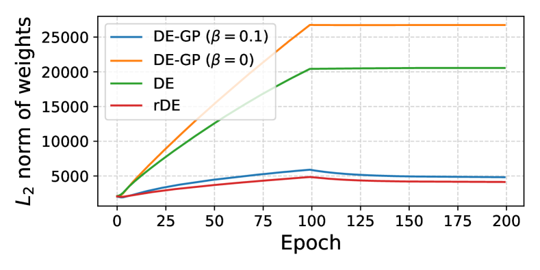
Figure 3: The $L_{2}$ norm of weights varies w.r.t. training step. The models are trained on CIFAR-10 with ResNet-20 architecture. DE-GP ($\beta=0$) finds solutions with high complexity and poor test accuracy (see Table 1), yet DE-GP ($\beta=0.1$) settles this.

4.3.3 An Extra Regularization on Weights

Generally, we usually introduce an $L_{2}$ regularization term on weights when optimizing over a parametric function class like DNNs. In this sense, we can generalize Equation 7 as:

$$\underset{{\bm{w}}_{1},...,{\bm{w}}_{M}}{\max}\,\mathcal{L} =\scalebox{1.0}{$\mathbb{E}_{f\sim q(f)}\left[\sum_{({\bm{x}}_{i},{\bm{y}}_{i})\in\mathcal{D}_{s}}\log p({\bm{y}}_{i}|f({\bm{x}}_{i}))\right]$}$$ (9)

$$\;\;\;\scalebox{1.0}{$-\,\alpha D_{\mathrm{KL}}\left[q(\mathbf{f}^{\tilde{\mathbf{X}}_{s}})\|p(\mathbf{f}^{\tilde{\mathbf{X}}_{s}})\right]-\beta\sum_{i}||{\bm{w}}_{i}||_{2}^{2}$},$$

where $\beta$ is set as 0 in default. Ideally, the KL divergence in Equation 9 is enough to help DE-GP to resist over-fitting (in function space). Its effectiveness is evidenced by the results in Figure 1, but we have empirically observed that it may lose efficacy when facing deep architectures like ResNets (He et al., 2016).

Specifically, we conducted a set of experiments with DE, rDE, and DE-GP using ResNet-20 architecture on CIFAR-10 benchmark (Krizhevsky et al., 2009). We plot how the $L_{2}$ norm of $\{{\bm{w}}_{i}\}_{i=1}^{M}$ varies w.r.t. training step in Figure 3 and display the comparison on test accuracy in Table 1.

An immediate conclusion is that the KL in Equation 9 cannot cause proper regularization effects on weights for DE-GP when using ResNet-20, thus the learned DE-GP suffers from high complexity and hence poor performance.

Having identified this, we suggest activating the $L_{2}$ weight regularization term in Equation 9 when handling deep architectures. In practice, we can set $\beta$ according to commonly used weight decay coefficient. We trained a DE-GP with $L_{2}$ weight regularization of intensity $0.1$ for the above case. The results in Figure 3 and Table 1 testify its effectiveness.

This extra regularization may introduce bias to the posterior inference corresponding to the imposed MC NN-GP prior. But, if we think of the extra regularization as a kind of extra prior knowledge, we can then justify it within the posterior regularization scheme (Ganchev et al., 2010) (see Appendix A).

Algorithm 1 The training of DE-GP

1:  Input: $\mathcal{D}$: dataset;

$\{g(\cdot,{\bm{w}}_{i})\}_{i=1}^{M}$

: a deep ensemble of size $M$; $k_{p}$: MC NN-GP prior kernel;

$\alpha,\beta$

: trade-off coefficients;

$\nu$

: distribution for sampling extra measurement points; $U$: number of MC samples for estimating the expected log-likelihood

2:  while not converged do

3:    

$\mathcal{D}_{s}=(\mathbf{X}_{s},\mathbf{Y}_{s})\subset\mathcal{D},\,\mathbf{X}_{\nu}\sim\nu,\tilde{\mathbf{X}}_{s}=\{\mathbf{X}_{s},\,\mathbf{X}_{\nu}\}$

4:    

$\mathbf{g}_{i}^{\tilde{\mathbf{X}}_{s}}=g(\tilde{\mathbf{X}}_{s},{\bm{w}}_{i}),\,i=1,...,M$

5:    

$\mathbf{m}^{\tilde{\mathbf{X}}_{s}}=\frac{1}{M}\sum_{i}\mathbf{g}_{i}^{\tilde{\mathbf{X}}_{s}}$

6:    

$\mathbf{k}^{\tilde{\mathbf{X}}_{s},\tilde{\mathbf{X}}_{s}}=\frac{1}{M}\sum_{i=1}^{M}(\mathbf{g}_{i}^{\tilde{\mathbf{X}}_{s}}-\mathbf{m}^{\tilde{\mathbf{X}}_{s}})(\mathbf{g}_{i}^{\tilde{\mathbf{X}}_{s}}-\mathbf{m}^{\tilde{\mathbf{X}}_{s}})^{\top}+\lambda\mathbf{I}_{|\tilde{\mathbf{X}}_{s}|C}$

7:    

$\mathbf{k}_{p}^{\tilde{\mathbf{X}}_{s},\tilde{\mathbf{X}}_{s}}=k_{p}(\tilde{\mathbf{X}}_{s},\tilde{\mathbf{X}}_{s})$

8:    

$\mathcal{L}_{1}=\frac{1}{U}\sum_{i=1}^{U}\sum_{({\bm{x}},{\bm{y}})\in\mathcal{D}_{s}}\log p({\bm{y}}|\mathbf{f}_{i}({\bm{x}})),\,\mathbf{f}_{i}\sim\mathcal{N}(\mathbf{m}^{\tilde{\mathbf{X}}_{s}},\mathbf{k}^{\tilde{\mathbf{X}}_{s},\tilde{\mathbf{X}}_{s}})$

9:    

$\mathcal{L}_{2}=D_{\mathrm{KL}}[\mathcal{N}(\mathbf{m}^{\tilde{\mathbf{X}}_{s}},\mathbf{k}^{\tilde{\mathbf{X}}_{s},\tilde{\mathbf{X}}_{s}})\|\mathcal{N}(\mathbf{0},\mathbf{k}_{p}^{\tilde{\mathbf{X}}_{s},\tilde{\mathbf{X}}_{s}})]$

10:    

$\mathcal{L}_{3}=\sum_{i}||{\bm{w}}_{i}||_{2}^{2}$

11:    

${\bm{w}}_{i}={\bm{w}}_{i}+\eta\nabla_{{\bm{w}}_{i}}(\mathcal{L}_{1}-\alpha\mathcal{L}_{2}-\beta\mathcal{L}_{3}),\,i=1,...,M$

12:  end while

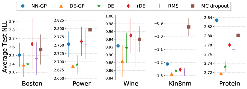
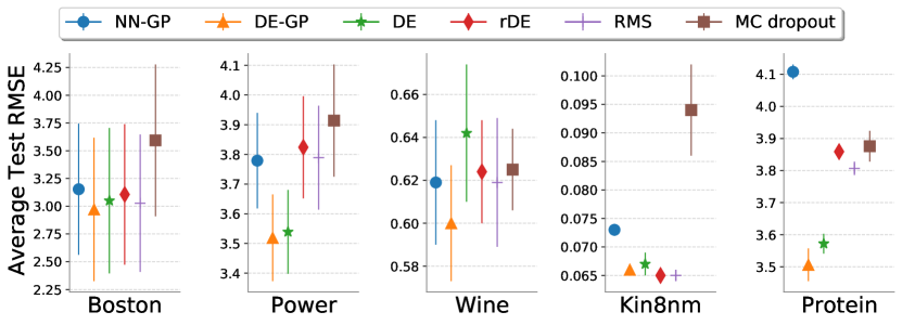
Figure 4: Comparison on average test NLL and RMSE on UCI regression problems. The lower the better.

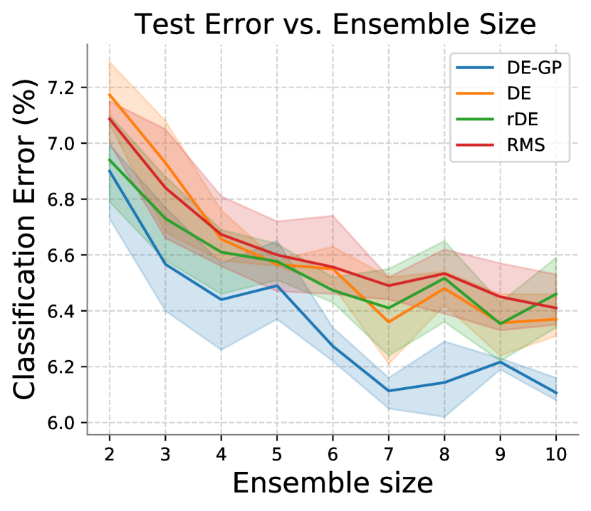
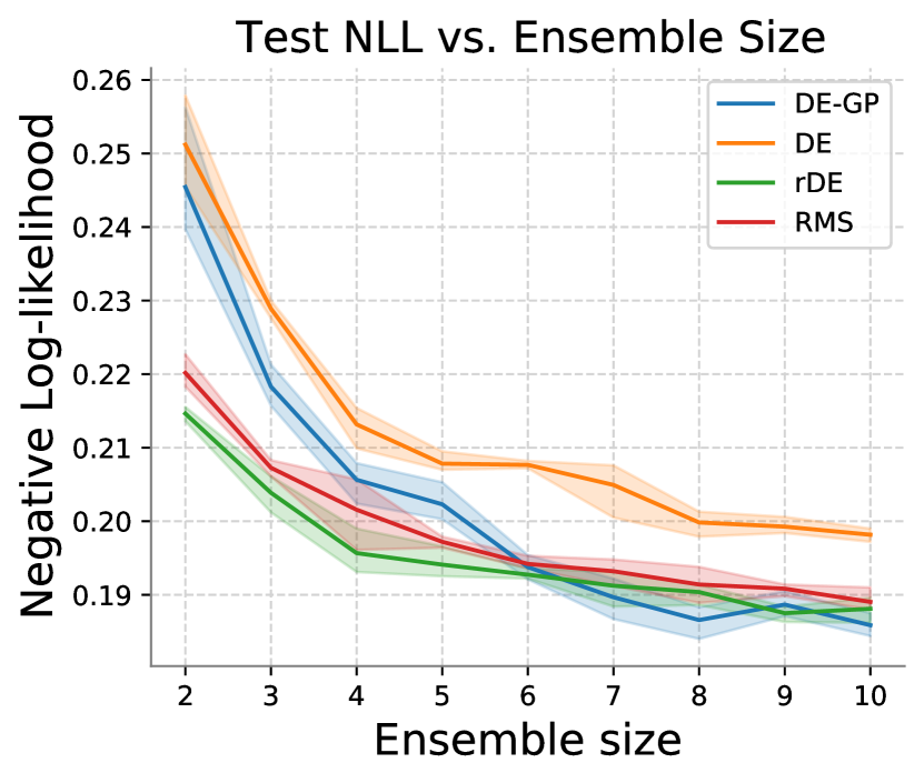
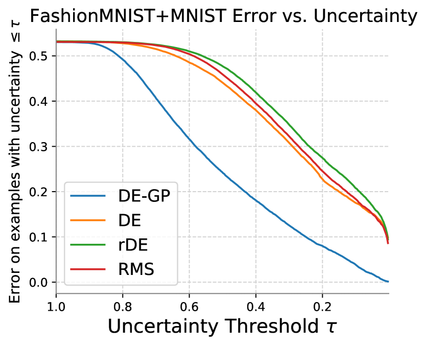
Figure 5: (Left): Test error varies w.r.t. ensemble size on Fashion-MNIST. (Middle): Test NLL varies w.r.t. ensemble size on Fashion-MNIST. (Right): Test error versus uncertainty plots for methods trained on Fashion-MNIST and tested on both Fashion-MNIST and MNIST. Ensemble size is fixed as 10.

4.4 Discussions

Diversity. The diversity among the ensemble members in function space is explicitly encouraged by the KL divergence term in Equation 9. Nonetheless, the expected log-likelihood in Equation 9 enforces each ensemble member to yield the same, correct outcomes for the training data. Thereby, the diversity mainly exists in the regions far away from the training data (see Figure 1). Yet, the diversity in DE does not have a clear theoretical support.

Efficiency. Compared to the overhead introduced by DNNs, the effort for estimating the KL in Equation 9 is negligible. The added cost of DE-GP primarily arises from the extra measurement points and the evaluation of the prior kernels. In practice, we use a small batch size for the extra measurement points. We build the MC NN-GP prior kernels with cheap architectures and perform MC estimation in parallel. Eventually, DE-GP is only marginally slower than DE.

Weight sharing. DE-GP does not care about how $g_{i}$ are parameterized, so we can perform weight sharing among $g_{i}$, for example, using a shared feature extractor and $M$ independent MLP classifiers to construct $M$ ensemble members (Deng et al., 2021). With shared weights, DE-GP is still likely to be reliable because our learning principle induces diversity in function space regardless of the weights. Experiments in Section 5.3 validate this.

Limitations. Despite being Bayesian in principle, DE-GP loses parallelisability. Nevertheless, it may be a common issue, e.g., the methods of (D’Angelo & Fortuin, 2021) also entail concurrent updates of the ensemble members.

5 Experiments

We perform extensive evaluation to demonstrate that DE-GP yields better uncertainty estimates than the baselines, while preserving non-degraded predictive performance. The baselines include DE, rDE, NN-GP, RMS, etc. In all experiments, we estimate the MC NN-GP prior kernels with $10$ MC samples and set the sampling distribution for extra measurement points $\nu$ as the uniform distribution over the data region. The number of MC samples for estimating the expected log-likelihood (i.e., $U$ in Algorithm 1) is $256$. Unless otherwise stated, we set the regularization constant $\lambda$ as $0.05$ times of the average eigenvalue of the central covariance matrices, and set the weight and bias variance for defining the MC NN-GP prior kernel at each layer as $2/\texttt{fan\_in}$ and $0.01$, where fan_in is the number of input features, as suggested by He et al. (2015).

5.1 Illustrative 1-D Regression

We build a regression problem with $8$ data from $y=\sin 2x+\epsilon,\epsilon\sim\mathcal{N}(0,0.2)$ as shown in Figure 2. The rightest datum is deliberately perturbed to cause data noise. For NN-GP, we analytically estimate the GP kernel and perform GP regression without training DNNs. For DE-GP, DE, and rDE, we train 50 MLPs. By default, we set $\alpha=1$, $\beta=0$.

Figure 2 and Figure 1 show the comparison on prediction and training efficiency. As shown, DE-GP delivers calibrated uncertainty estimates across settings, on par with the non-parametric Bayesian baseline NN-GP. Yet, DE and rDE suffer from degeneracy issue as the dimension of weights increases. Though NN-GP outperforms other methods, the involved analytical GP regression may have scalability and effectiveness issues when facing modern architectures (Novak et al., 2018), while DE-GP does not suffer from them.

Table 1: Test accuracy comparison on CIFAR-10. Results are summarized over 8 trials.

Architecture	DE-GP ($\beta=0.1$)	DE-GP ($\beta=0$)	DE	rDE	RMS
ResNet-20	94.67$\pm$0.04%	93.71$\pm$0.06%	93.43$\pm$0.08%	94.58$\pm$0.05%	93.63$\pm$0.07%
ResNet-56	95.55$\pm$0.04%	94.24$\pm$0.07%	94.04$\pm$0.07%	95.56$\pm$0.06%	94.45$\pm$0.03%

Figure 6: Test error versus uncertainty plots for methods trained on CIFAR-10 and tested on both CIFAR-10 and SVHN with ResNet-20 (Left) or ResNet-56 (Right) architecture.

Figure 7: Expected Calibration Error on CIFAR-10 corruptions for models trained with ResNet-20 (Left) or ResNet-56 (Right) architecture. We summarize the results across 19 types of skew in each box.

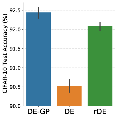
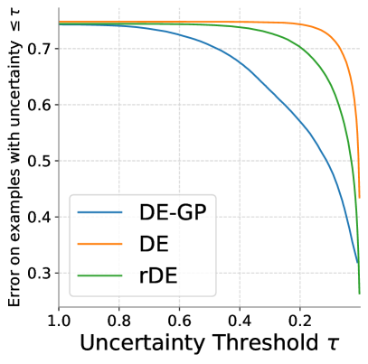
Figure 8: In-distribution test accuracy (Left) and error versus uncertainty plots on the combination CIFAR-10 and SVHN (Right) under weight sharing. (ResNet-20)

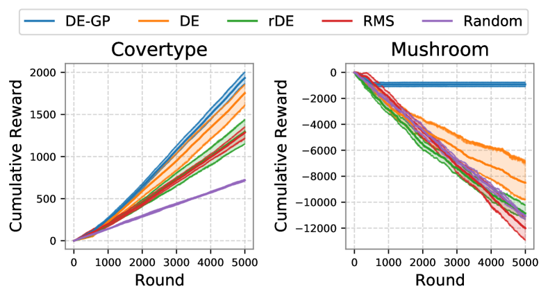
Figure 9: Cumulative reward varies w.r.t. round on Covertype (Left) and Mushroom (Right). Random corresponds to the Uniform algorithm. Summarized over 5 trials.

5.2 UCI Regression

We then assess DE-GP on 5 UCI real-valued regression problems. The used architecture is a MLP with 2 hidden layers of 256 units and ReLU activation. 10 networks are trained for DE, DE-GP and other variants. For DE-GP, we set $\beta=0$ and tune $\alpha$ according to validation sets.

We perform cross validation with 5 splits. Figure 4 shows the results. DE-GP surpasses or approaches the baselines across scenarios in aspects of both test negative log-likelihood (NLL) and test root mean square error (RMSE). DE-GP even beats NN-GP, which is probably attributed to that the variational family specified by DE enjoys the beneficial inductive bias of practically sized SGD-trained DNNs, and DE-GP can flexibly trade off between the likelihood and the prior by tuning $\alpha$.

5.3 Classification on Fashion-MNIST and CIFAR-10

In the classification experiments, we augment the data log-likelihood (i.e., the first term in Equation 9) with a trainable temperature to tackle oversmoothing and avoid underconfidence.

Fashion-MNIST. We use a widened LeNet5 architecture with batch normalizations (BNs) (Ioffe & Szegedy, 2015) for the Fashion-MNIST dataset (Xiao et al., 2017). Considering the inefficiency of NN-GP, we mainly compare DE-GP to DE, rDE, and RMS. We set $\alpha$ as well as the regularization coefficients for rDE and RMS all as $0.1$ according to validation accuracy. For DE-GP, we use $\beta=0$ given the limited capacity of the architecture. The in-distribution performance is averaged over 8 runs. Figure 5-(Left) and Figure 5-(Middle) display how ensemble size impacts the test results. Surprisingly, the test error of DE-GP is even lower than the baselines, and its test NLL decreases rapidly as the ensemble size increases.

Besides, to compare the quality of uncertainty estimates, we use the trained models to make prediction and quantify epistemic uncertainty for both the in-distribution test set and the out-of-distribution (OOD) MNIST test set. All predictions on OOD data are regarded as wrong. The epistemic uncertainty is estimated by the mutual information between the prediction and the variable function:

$$\small\mathcal{I}(f,y|{\bm{x}},\mathcal{D})\approx H\left(\frac{1}{S}\sum_{s=1}^{S}p(y|f_{s}({\bm{x}}))\right)-\frac{1}{S}\sum_{s=1}^{S}H\left(p(y|f_{s}({\bm{x}}))\right),$$ (10)

where $H$ indicates Shannon entropy, with $f_{s}=g(\cdot,{\bm{w}}_{s})$ for DE, rDE, and RMS, and $f_{s}\sim q(f;{\bm{w}}_{1},...,{\bm{w}}_{M})$ for DE-GP. This is a naive extension of the weight uncertainty-based mutual epistemic uncertainty. We normalize the uncertainty estimates into $[0,1]$. For each threshold $\tau\in[0,1]$, we plot the average test error for data with $\leq\tau$ uncertainty in Figure 5-(Right). It is prominent that under various uncertainty thresholds, DE-GP makes fewer mistakes than the baselines, implying that DE-GP succeeds to assign relatively higher uncertainty for the OOD data.

CIFAR-10. Next, we apply DE-GP to the real-world image classification task CIFAR-10. We consider the popular ResNet architectures including ResNet-20 and ResNet-56. The ensemble size is fixed as $10$. We split the data as training set, validation set, and test set of size 45000, 5000, 10000, respectively. We set $\beta=0.1$, equivalent with the regularization coefficient on weight in rDE. We set $\alpha=0.1$ according to an ablation study in Section B.5. We use a lite ResNet-20 architecture without BNs and residual connections to set up the MC NN-GP prior kernel for both the ResNet-20 and ResNet-56 based variational posteriors.

We present the in-distribution test accuracy in Table 1 and the error versus uncertainty plots on the combination of CIFAR-10 and SVHN test sets in Figure 6. DE-GP is on par with the practically-used, competing rDE in aspect of test accuracy. DE-GP ($\beta=0$) shows unsatisfactory test accuracy, verifying the necessity of incorporating an extra weight-space regularization term when using deep networks. The error versus uncertainty plots are similar to those for Fashion-MNIST, substantiating the universality of DE-GP.

We further test the trained methods on CIFAR-10 corruptions (Hendrycks & Dietterich, 2018), a challenging OOD generalization/robustness benchmark for deep models. As shown in Figure 7 and Section B.3, DE-GP reveals smaller Expected Calibration Error (ECE) (Guo et al., 2017) and lower NLL at various levels of skew, reflecting its ability to make conservative predictions under corruptions.

More results for the deeper ResNet-110 architecture and the more challenging CIFAR-100 benchmark are provided in Section B.3 and Section B.4.

Weight Sharing. We build a ResNet-20 with 10 classification heads and a shared feature extraction module to evaluate the methods under weight sharing. We set a larger value for $\alpha$ for DE-GP to induce higher magnitudes of functional diversity. The test accuracy (over 8 trials) and error versus uncertainty plots on CIFAR-10 are illustrated in Figure 9. We exclude RMS from the comparison as it assumes i.i.d. ensemble members which may be incompatible with weight sharing. DE-GP benefits from a function-space diversity-promoting term, hence performs better than DE and rDE, which purely hinge on the randomness in weight space.

5.4 Contextual Bandit

Finally, we apply DE-GP to contextual bandit, an important decision-making task where the uncertainty helps to guide exploration. Following (Osband et al., 2016), we use DE-GP to achieve efficient exploration inspired by Thompson sampling. We reuse most of the settings for UCI regression. We leverage the GenRL library to build two contextual bandit problems Covertype and Mushroom (Riquelme et al., 2018). The cumulative reward is depicted in Figure 9. As desired, DE-GP offers better uncertainty estimates and hence beats the baselines by clear margins. The potential of DE-GP in more reinforcement learning and Bayesian optimization scenarios deserves future investigation.

6 Conclusion

In this work, we address the unreliability issue of the uncertainty estimates of Deep Ensemble by defining a Gaussian process with Deep Ensemble and training the model under the principle of functional variational inference. Doing so, we have successfully related Deep Ensemble to Bayesian inference to enjoy principled Bayesian uncertainty. We offer recipes to make the training feasible, and further identify the necessity of incorporating an extra weight-space regularization term when adopting deep architectures. Our method can be implemented easily and efficiently. Extensive experiments validate the effectiveness of our method. We hope this work may shed light on the development of better Bayesian deep learning approaches.

Appendix A An Explanation for the Weight-space Regularization

Posterior regularization (Ganchev et al., 2010; Zhu et al., 2014) provides a workaround for Bayesian approaches to impose extra prior knowledge. We can apply posterior regularization to functional variational inference by solving:

$$\small\max_{q(f)}\mathcal{L}=\mathbb{E}_{q(f)}[\log p(\mathcal{D}|f)]-D_{\mathrm{KL}}[q(f)\|p(f)]\;\text{s.t.:}\;q(f)\in Q.$$ (11)

$Q=\{q(f)|\mathbb{E}_{q(f)}\Omega(f)\leq{0}\}$ is a valid set defined in terms of a functional $\Omega$ which delivers some statistic of interest of a function. For tractable optimization, we can slack the constraint as a penalty:

$$\small\max_{q(f)}\mathcal{L}^{\prime}=\mathcal{L}-\beta\max\{\mathbb{E}_{q(f)}\Omega(f),0\},$$ (12)

where $\beta$ is a trade-off coefficient.

We next show that the extra weight-space regularization can be derived by imposing the extra prior that functions drawn from DE-GP should generalize well to the learning of DE-GP given the above paradigm.

Binary classification In the binary classification scenario, $y\in\{-1,1\}$ and $f,g_{i}:\mathcal{X}\rightarrow\mathbb{R}$. We use $0$-$1$ loss $\ell(f({\bm{x}}),y)=\mathbf{1}_{y\neq\text{sign}(f({\bm{x}}))}$ to measure the classification error on one datum. We assume an underlying distribution $\mu=\mu({\bm{x}},y)$ supported on $\mathcal{X}\times\{-1,1\}$ for generating the training data $\mathcal{D}$, based on which we can define the true risk of a function (hypothesis) $f$: $R(f):=\mathbb{E}_{({\bm{x}},y)\sim\mu}\ell(f({\bm{x}}),y)$. We set $\mathbb{E}_{q(f)}\Omega(f):=\mathbb{E}_{q(f)}R(f)$ in the seek of a posterior over functions that can generalize well.

By definition, a hypothesis sample $f\sim q(f)=\mathcal{GP}(m({\bm{x}}),k({\bm{x}},{\bm{x}}^{\prime}))$ can be decomposed as $f({\bm{x}})=\frac{1}{M}\sum_{i=1}^{M}g_{i}({\bm{x}})+\zeta({\bm{x}})$ with $\zeta({\bm{x}})\sim\mathcal{GP}(0,k({\bm{x}},{\bm{x}}^{\prime}))$. If $\text{sign}(f({\bm{x}}))\neq y$, it is impossible that $\text{sign}(g_{1}({\bm{x}}))=y$, …, $\text{sign}(g_{M}({\bm{x}}))=y$, and $\text{sign}(\zeta({\bm{x}}))=y$ all hold. In other words,

$$\small{\ell(f({\bm{x}}),y)\leq\sum_{i=1}^{M}[\ell(g_{i}({\bm{x}}),y)]+\ell(\zeta({\bm{x}}),y).}$$ (13)

We can further re-parameterize $\zeta({\bm{x}})$ as $\zeta({\bm{x}})=\frac{1}{\sqrt{M}}\sum_{i=1}^{M}\epsilon_{i}(g_{i}({\bm{x}})-m({\bm{x}}))+\sqrt{\lambda}\epsilon_{0},\epsilon_{i}\sim\mathcal{N}(0,1),i=0,...,M$, which is essentially a real-valued random function symmetric around 0. Thus, for any $({\bm{x}},y)\sim\mu$, we have $\mathbb{E}_{q(f)}\ell(\zeta({\bm{x}}),y)=\mathbb{E}_{\epsilon_{0},...,\epsilon_{M}}\ell(\zeta({\bm{x}}),y)=1/2$. As a result,

$$\mathbb{E}_{q(f)}R(f) \leq\mathbb{E}_{q(f)}\mathbb{E}_{({\bm{x}},y)\sim\mu}\sum_{i=1}^{M}[\ell(g_{i}({\bm{x}}),y)]+\mathbb{E}_{({\bm{x}},y)\sim\mu}[1/2]$$ (14)

$$=\sum_{i=1}^{M}[R(g_{i})]+1/2.$$

Namely, the expected generalization error of the approximately posteriori functions can be bounded from above by those of the DNN basis functions. Recalling the theoretical and empirical results showing that DNNs’ generalization error $R(g_{i})$ can be decreased by controlling model capacity in terms of norm-based regularization $\min_{{\bm{w}}_{i}}||{\bm{w}}_{i}||_{2}^{2}$ (Neyshabur et al., 2015, 2017; Bartlett et al., 2017; Jiang et al., 2019), we obtain an explanation for the extra weight-space regularization.

Multi-class Classification In the multi-class classification scenario where $y\in\{1,2,...,C\}$ and $f,g_{i}:\mathcal{X}\rightarrow\mathbb{R}^{C}$, we use the loss $\ell(f({\bm{x}}),y)=\mathbf{1}_{f({\bm{x}})[y]<\max_{y^{\prime}\neq y}f({\bm{x}})[y^{\prime}]}$ to measure prediction error where $f({\bm{x}})[j]$ denotes $j$-th coordinate of $f({\bm{x}})$. The distinct difference between this scenario and the binary classification scenario is that in this setting, $\zeta({\bm{x}})$ is a vector-valued function:

$$\small\zeta({\bm{x}})=\frac{1}{\sqrt{M}}\sum_{i=1}^{M}\epsilon_{i}(g_{i}({\bm{x}})-m({\bm{x}}))+\sqrt{\lambda}\bm{\epsilon}_{0},$$ (15)

where $\bm{\epsilon}_{0}\sim\mathcal{N}(\mathbf{0},\mathbf{I}_{C})$ and $\epsilon_{i}\sim\mathcal{N}(0,1),i=1,...,M$. We then make a mild assumption to simplify the analysis.

Assumption 1.

For any $({\bm{x}},y)\in\mu$, the elements on the diagonal of $k({\bm{x}},{\bm{x}})$ have the same value.

This assumption implies that for any $j,j^{\prime}\in\{1,...,C\}$,

$$\small\frac{1}{M}\sum_{i=1}^{M}(g_{i}({\bm{x}})[j]-m({\bm{x}})[j])^{2}+\lambda=\frac{1}{M}\sum_{i=1}^{M}(g_{i}({\bm{x}})[j^{\prime}]-m({\bm{x}})[j^{\prime}])^{2}+\lambda.$$ (16)

I.e.,

$$\small\sum_{i=1}^{M}(g_{i}({\bm{x}})[j]-m({\bm{x}})[j])^{2}=\sum_{i=1}^{M}(g_{i}({\bm{x}})[j^{\prime}]-m({\bm{x}})[j^{\prime}])^{2}.$$ (17)

Therefore, $\zeta({\bm{x}})$ possesses the same variance across its output coordinates and becomes a random guess classifier. Based on this, we have $\mathbb{E}_{q(f)}\ell(\zeta({\bm{x}}),y)=\mathbb{E}_{\epsilon_{0},...,\epsilon_{M}}\ell(\zeta({\bm{x}}),y)=(C-1)/C$. We can then derive a similar conclusion to that in the binary classification.

The validity of Assumption 1. When the data dimension $|\mathcal{X}|$ is high and the number of training data $n$ is finitely large, with zero probability the sampled data $({\bm{x}},y)\sim\mu$ resides in the training set. Therefore, only the KL divergence term of the fELBO explicitly affects the predictive uncertainty at ${\bm{x}}$. Because the MC NN-GP prior possesses a diagonal structure, it is hence reasonable to make the above assumption.

Appendix B More of Experiments

We provide experimental details and more results in this section.

B.1 Detailed Settings

Illustrative regression. For the problem on $y=\sin 2x+\epsilon,\epsilon\sim\mathcal{N}(0,0.1)$, we randomly sample 8 data points from $[-1.5,1.5]$. We add $-1.2$ to the target value of the rightest data point to introduce strong data noise. For optimizing the ensemble members, we use a SGD optimizer with $0.9$ momentum and $0.001$ learning rate. The learning rate follows a cosine decay schedule. The optimization takes $1000$ iterations. The extra measurement points are uniformly sampled from $[-2,2]$. The regularization constant $\lambda$ is set as $1e-4$ times of the average eigenvalue of the central covariance matrices.

UCI regression. We pre-process the UCI data by standard normalization. We set the variance for data noise and the weight variance for the prior kernel following (Pearce et al., 2020). The batch size for stochastic training is $256$. We use an Adam optimizer to optimize for $1000$ epochs. The learning rate is initialized as $0.01$ and decays by $0.99$ every $5$ epochs.

Fashion-MNIST classification. The used architecture is Conv(32, 3, 1)-BN-ReLU-MaxPool(2)-Conv(64, 3, 0)-BN-ReLU-MaxPool(2)-Linear(256)-ReLU-Linear(10), where Conv($x$, $y$, $z$) represents a 2D convolution with $x$ output channels, kernel size $y$, and padding $z$. The batch size for training data is $64$. We do not use extra measurement points here. We use an SGD optimizer to optimize for $24$ epochs. The learning rate is initialized as $0.1$ and follows a cosine decay schedule. We use an Adam optimizer with $1e-3$ learning rate to optimize the temperature. We use $1000$ MC samples to estimate the posterior predictive and the epistemic uncertainty, because the involved computation is only the cheap softmax transformation on the sampled function values.

CIFAR-10 classification. We perform data augmentation including random horizontal flip and random crop. The batch size for training data is $128$. We do not use extra measurement points here. We use a SGD optimizer with $0.9$ momentum to optimize for $200$ epochs. The learning rate is initialized as $0.1$ and decays by $0.1$ at $100$-th and $150$-th epochs. We use an Adam optimizer with $1e-3$ learning rate to optimize the temperature. We use $1000$ MC samples to estimate the posterior predictive and the epistemic uncertainty. Suggested by (Ovadia et al., 2019; He et al., 2020), we train models on CIFAR-10, and test them on the combination of CIFAR-10 and SVHN test sets. This is a standard benchmark for evaluating the uncertainty on OOD data.

Contextual bandit. We use MLPs with 2 hidden layers of 256 units. The batch size for training data is 512. We do not use extra measurement points here. We update the model (i.e., the agent) for $100$ epochs with an Adam optimizer every $50$ rounds. We set $\alpha=1$ and $\beta=0$ without tuning. DE, rDE, and RMS all randomly choose an ensemble member at per iteration, but our method randomly draws a sample from the defined Gaussian process for decision. This is actually emulating Thompson Sampling and advocated by Bootstrapped DQN (Osband et al., 2016). “Random” baseline corresponds to the Uniform algorithm.

MLPs w/o hidden layers

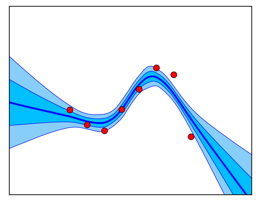
MLPs w/ 1 hidden layer

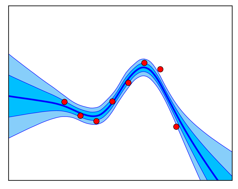
MLPs w 2 hidden layers

MLPs w 3 hidden layers

Figure 10: Results of DE-GP without using extra measurement points. The settings are equivalent to those in Figure 2.

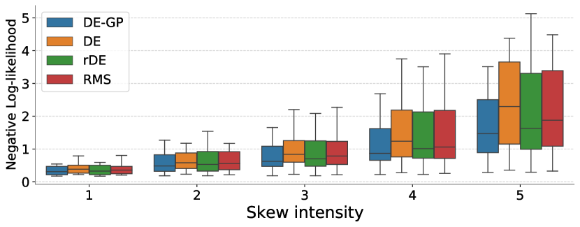
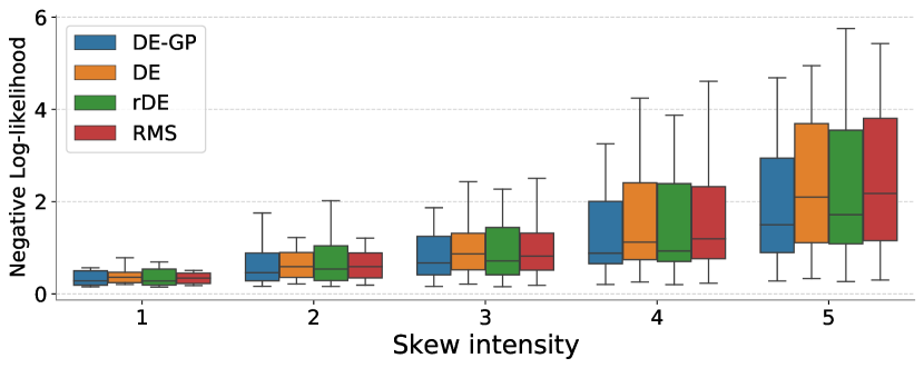
Figure 11: Negative log-likelihood on CIFAR-10 corruptions for models trained with ResNet-20 (Left) or ResNet-56 (Right) architecture. We summarize the results across 19 types of skew in each box.

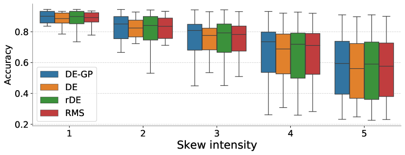
Figure 12: Test accuracy on CIFAR-10 corruptions for models trained with ResNet-20 (Left) or ResNet-56 (Right) architecture. We summarize the results across 19 types of skew in each box.

B.2 Results of DE-GP without using Extra Measurement Points

We depict the results of DE-GP without using extra measurement points on $y=\sin 2x+\epsilon,\epsilon\sim\mathcal{N}(0,0.2)$ problem in Figure 10. The results are promising.

B.3 More Results on CIFAR-10 Classification

We plot the negative log-likelihood and test accuracy on CIFAR-10 corruptions for models trained with ResNet-20 and ResNet-56 in Figure 11 and Figure 12. As shown, DE-GP outperforms the baselines in aspect of negative log-likelihood, but yields similar test accuracy to the baselines. Recapping the results in Figure 7, DE-GP indeed has improved OOD robustness, but may still face problems in OOD generalization.

We then conduct experiments with the deeper ResNet-110 architecture. Due to resource constraint, we use $5$ ensemble members. The other settings are roughly the same as those for ResNet-56. The results are offered in Figure 13, which validate the effectiveness of DE-GP for large networks.

Figure 13: (Left): Expected Calibration Error on CIFAR-10 corruptions for models trained with ResNet-110 architecture. We summarize the results across 19 types of skew in each box. (Right): Test error versus uncertainty plots for methods trained on CIFAR-10 and tested on both CIFAR-10 and SVHN with ResNet-110 architecture. Ensemble size is fixed as 5 for these experiments.

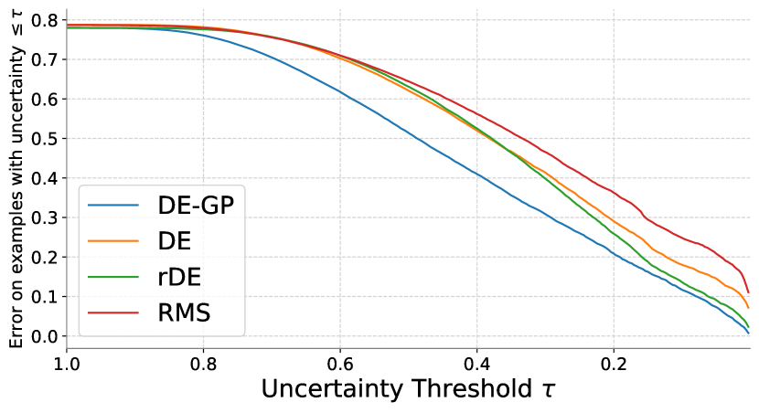
Figure 14: Test error versus uncertainty plots for methods trained on CIFAR-100 and tested on both CIFAR-100 and SVHN with ResNet-20 (Left) or ResNet-56 (Right) architecture.

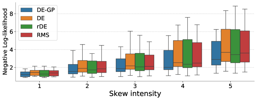
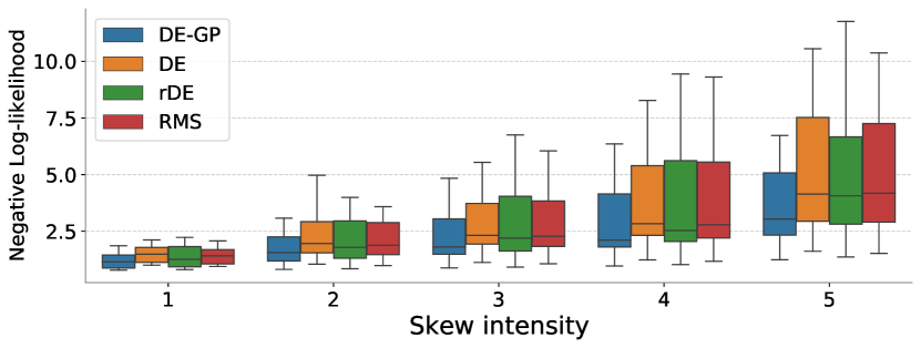
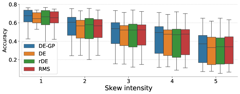
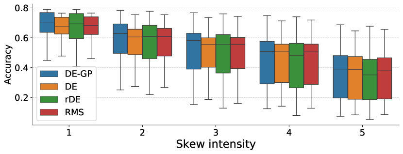
Figure 15: First row: test NLL on CIFAR-100 corruptions for models trained with ResNet-20 (Left) or ResNet-56 (Right) architecture. Second row: test accuracy on CIFAR-100 corruptions for models trained with ResNet-20 (Left) or ResNet-56 (Right) architecture. We summarize the results across 19 types of skew in each box.

B.4 Results on CIFAR-100

We further perform experiments on the more challenging CIFAR-100 benchmark. We present the in-distribution test accuracy of DE-GP as well as the baselines in Table 2. We can see that DE-GP ($\beta=0.1$) is still on par with rDE. We depict the error versus uncertainty plots on the combination of CIFAR-100 and SVHN test sets in Figure 14. It is shown that the uncertainty estimates yielded by DE-GP for OOD data are more calibrated than the baselines. We further test the trained methods on CIFAR-100 corruptions (Hendrycks & Dietterich, 2018), and present the comparisons in aspects of test accuracy and NLL in Figure 15. It is evident that DE-GP reveals lower NLL than the baselines at various levels of skew.

Table 2: Test accuracy comparison on CIFAR-100.

Architecture	DE-GP ($\beta=0.1$)	DE	rDE	RMS
ResNet-20	76.59%	74.14%	76.81%	75.08%
ResNet-56	79.51%	76.46%	79.21%	76.77%

B.5 Ablation Study on $\alpha$

We have conducted an ablation study on $\alpha$ (using ResNet-20 on CIFAR-10). The results are presented in Table 3. We can see that DE-GP is not sensitive to the value of $\alpha$. We in practice set $\alpha=0.1$ in the CIFAR experiments. We did not use a smaller $\alpha$ as it may result in colder posteriors and in turn worse uncertainty estimates.

Table 3: Ablation study on $\alpha$ for DE-GP ($\beta=0.1$) (using ResNet-20 on CIFAR-10).

$\alpha$	0.1	0.05	0.01	0.005
Accuracy	94.67$\pm$0.09%	94.66$\pm$0.07%	94.67$\pm$0.04%	94.83$\pm$0.10%

B.6 Ablation Study on the Architecture of Prior Kernel

We perform an ablation study on the architecture for defining the prior MC NN-GP kernel, with the results listed in Table 4. Surprisingly, using the cheap ResNet-20 architecture results in DE-GP with better test accuracy. We deduce this is because a deeper prior architecture induces more complex, black-box correlation for the function, which may lead to over-regularization.

Table 4: Ablation study on the architecture of the prior MC NN-GP kernel.

	ResNet-20	ResNet-56	ResNet-110
ResNet-56 (10 ensemble member)	95.50%	95.28%	-
ResNet-110 (5 ensemble member)	95.54%	-	94.87%

References

- Bartlett et al. (2017) Bartlett, P. L., Foster, D. J., and Telgarsky, M. J. Spectrally-normalized margin bounds for neural networks. Advances in Neural Information Processing Systems, 30:6240–6249, 2017.
- Blundell et al. (2015) Blundell, C., Cornebise, J., Kavukcuoglu, K., and Wierstra, D. Weight uncertainty in neural network. In International Conference on Machine Learning, pp. 1613–1622, 2015.
- Burt et al. (2020) Burt, D. R., Ober, S. W., Garriga-Alonso, A., and van der Wilk, M. Understanding variational inference in function-space. In Third Symposium on Advances in Approximate Bayesian Inference, 2020.
- Chen et al. (2014) Chen, T., Fox, E., and Guestrin, C. Stochastic gradient hamiltonian monte carlo. In International conference on machine learning, pp. 1683–1691. PMLR, 2014.
- D’Angelo & Fortuin (2021) D’Angelo, F. and Fortuin, V. Repulsive deep ensembles are bayesian. arXiv preprint arXiv:2106.11642, 2021.
- Deng et al. (2020) Deng, Z., Zhang, H., Yang, X., Dong, Y., and Zhu, J. Bayesadapter: Being bayesian, inexpensively and reliably, via bayesian fine-tuning. arXiv preprint arXiv:2010.01979, 2020.
- Deng et al. (2021) Deng, Z., Yang, X., Xu, S., Su, H., and Zhu, J. Libre: A practical bayesian approach to adversarial detection. In Proceedings of the IEEE/CVF Conference on Computer Vision and Pattern Recognition (CVPR), pp. 972–982, June 2021.
- Dusenberry et al. (2020) Dusenberry, M., Jerfel, G., Wen, Y., Ma, Y., Snoek, J., Heller, K., Lakshminarayanan, B., and Tran, D. Efficient and scalable bayesian neural nets with rank-1 factors. In International conference on machine learning, pp. 2782–2792. PMLR, 2020.
- Fort et al. (2019) Fort, S., Hu, H., and Lakshminarayanan, B. Deep ensembles: A loss landscape perspective. arXiv preprint arXiv:1912.02757, 2019.
- Gal & Ghahramani (2016) Gal, Y. and Ghahramani, Z. Dropout as a Bayesian approximation: Representing model uncertainty in deep learning. In International Conference on Machine Learning, pp. 1050–1059, 2016.
- Ganchev et al. (2010) Ganchev, K., Graça, J., Gillenwater, J., and Taskar, B. Posterior regularization for structured latent variable models. The Journal of Machine Learning Research, 11:2001–2049, 2010.
- Graves (2011) Graves, A. Practical variational inference for neural networks. In Advances in Neural Information Processing Systems, pp. 2348–2356, 2011.
- Guo et al. (2017) Guo, C., Pleiss, G., Sun, Y., and Weinberger, K. Q. On calibration of modern neural networks. In International Conference on Machine Learning, pp. 1321–1330. PMLR, 2017.
- Harville (1998) Harville, D. A. Matrix algebra from a statistician’s perspective, 1998.
- He et al. (2020) He, B., Lakshminarayanan, B., and Teh, Y. W. Bayesian deep ensembles via the neural tangent kernel. In Advances in Neural Information Processing Systems, volume 33, 2020.
- He et al. (2015) He, K., Zhang, X., Ren, S., and Sun, J. Delving deep into rectifiers: Surpassing human-level performance on imagenet classification. In Proceedings of the IEEE international conference on computer vision, pp. 1026–1034, 2015.
- He et al. (2016) He, K., Zhang, X., Ren, S., and Sun, J. Deep residual learning for image recognition. In Proceedings of the IEEE Conference on Computer Vision and Pattern Recognition, pp. 770–778, 2016.
- Hendrycks & Dietterich (2018) Hendrycks, D. and Dietterich, T. Benchmarking neural network robustness to common corruptions and perturbations. In International Conference on Learning Representations, 2018.
- Hernández-Lobato & Adams (2015) Hernández-Lobato, J. M. and Adams, R. Probabilistic backpropagation for scalable learning of Bayesian neural networks. In International Conference on Machine Learning, pp. 1861–1869, 2015.
- Hinton & Van Camp (1993) Hinton, G. and Van Camp, D. Keeping neural networks simple by minimizing the description length of the weights. In ACM Conference on Computational Learning Theory, 1993.
- Hron et al. (2018) Hron, J., Matthews, A., and Ghahramani, Z. Variational bayesian dropout: pitfalls and fixes. In International Conference on Machine Learning, pp. 2019–2028. PMLR, 2018.
- Ioffe & Szegedy (2015) Ioffe, S. and Szegedy, C. Batch normalization: Accelerating deep network training by reducing internal covariate shift. In International conference on machine learning, pp. 448–456. PMLR, 2015.
- Izmailov et al. (2020) Izmailov, P., Maddox, W. J., Kirichenko, P., Garipov, T., Vetrov, D., and Wilson, A. G. Subspace inference for bayesian deep learning. In Uncertainty in Artificial Intelligence, pp. 1169–1179. PMLR, 2020.
- Jiang et al. (2019) Jiang, Y., Neyshabur, B., Mobahi, H., Krishnan, D., and Bengio, S. Fantastic generalization measures and where to find them. In International Conference on Learning Representations, 2019.
- Khan et al. (2018) Khan, M. E., Nielsen, D., Tangkaratt, V., Lin, W., Gal, Y., and Srivastava, A. Fast and scalable Bayesian deep learning by weight-perturbation in adam. In International Conference on Machine Learning, pp. 2616–2625, 2018.
- Khan et al. (2019) Khan, M. E. E., Immer, A., Abedi, E., and Korzepa, M. Approximate inference turns deep networks into gaussian processes. Advances in Neural Information Processing Systems, 32, 2019.
- Krizhevsky et al. (2009) Krizhevsky, A., Hinton, G., et al. Learning multiple layers of features from tiny images. 2009.
- Lakshminarayanan et al. (2017) Lakshminarayanan, B., Pritzel, A., and Blundell, C. Simple and scalable predictive uncertainty estimation using deep ensembles. In Advances in Neural Information Processing Systems, pp. 6402–6413, 2017.
- Langley (2000) Langley, P. Crafting papers on machine learning. In Langley, P. (ed.), Proceedings of the 17th International Conference on Machine Learning (ICML 2000), pp. 1207–1216, Stanford, CA, 2000. Morgan Kaufmann.
- Lee et al. (2018) Lee, J., Bahri, Y., Novak, R., Schoenholz, S. S., Pennington, J., and Sohl-Dickstein, J. Deep neural networks as gaussian processes. In International Conference on Learning Representations, 2018.
- Liu & Wang (2016) Liu, Q. and Wang, D. Stein variational gradient descent: A general purpose Bayesian inference algorithm. In Advances in Neural Information Processing Systems, pp. 2378–2386, 2016.
- Louizos & Welling (2016) Louizos, C. and Welling, M. Structured and efficient variational deep learning with matrix gaussian posteriors. In International Conference on Machine Learning, pp. 1708–1716, 2016.
- Lu & Van Roy (2017) Lu, X. and Van Roy, B. Ensemble sampling. In NIPS, 2017.
- MacKay (1992) MacKay, D. J. A practical Bayesian framework for backpropagation networks. Neural Computation, 4(3):448–472, 1992.
- Mackay (1992) Mackay, D. J. C. Bayesian methods for adaptive models. PhD thesis, California Institute of Technology, 1992.
- Maddox et al. (2019) Maddox, W. J., Izmailov, P., Garipov, T., Vetrov, D. P., and Wilson, A. G. A simple baseline for bayesian uncertainty in deep learning. In Advances in Neural Information Processing Systems, pp. 13153–13164, 2019.
- Matthews et al. (2017) Matthews, A. G. d. G., Hron, J., Turner, R. E., and Ghahramani, Z. Sample-then-optimize posterior sampling for bayesian linear models. In NeurIPS Workshop on Advances in Approximate Bayesian Inference, 2017.
- Neal (1995) Neal, R. M. Bayesian Learning for Neural Networks. PhD thesis, University of Toronto, 1995.
- Neal (1996) Neal, R. M. Priors for infinite networks. In Bayesian Learning for Neural Networks, pp. 29–53. Springer, 1996.
- Neyshabur et al. (2015) Neyshabur, B., Tomioka, R., and Srebro, N. Norm-based capacity control in neural networks. In Conference on Learning Theory, pp. 1376–1401. PMLR, 2015.
- Neyshabur et al. (2017) Neyshabur, B., Bhojanapalli, S., Mcallester, D., and Srebro, N. Exploring generalization in deep learning. Advances in Neural Information Processing Systems, 30:5947–5956, 2017.
- Novak et al. (2018) Novak, R., Xiao, L., Bahri, Y., Lee, J., Yang, G., Hron, J., Abolafia, D. A., Pennington, J., and Sohl-dickstein, J. Bayesian deep convolutional networks with many channels are gaussian processes. In International Conference on Learning Representations, 2018.
- Osband et al. (2016) Osband, I., Blundell, C., Pritzel, A., and Van Roy, B. Deep exploration via bootstrapped dqn. Advances in neural information processing systems, 29:4026–4034, 2016.
- Osband et al. (2018) Osband, I., Aslanides, J., and Cassirer, A. Randomized prior functions for deep reinforcement learning. Advances in Neural Information Processing Systems, 31, 2018.
- Ovadia et al. (2019) Ovadia, Y., Fertig, E., Ren, J., Nado, Z., Sculley, D., Nowozin, S., Dillon, J., Lakshminarayanan, B., and Snoek, J. Can you trust your model’s uncertainty? evaluating predictive uncertainty under dataset shift. Advances in Neural Information Processing Systems, 32:13991–14002, 2019.
- Pearce et al. (2020) Pearce, T., Leibfried, F., and Brintrup, A. Uncertainty in neural networks: Approximately bayesian ensembling. In International conference on artificial intelligence and statistics, pp. 234–244. PMLR, 2020.
- Riquelme et al. (2018) Riquelme, C., Tucker, G., and Snoek, J. Deep bayesian bandits showdown: An empirical comparison of bayesian deep networks for thompson sampling. In International Conference on Learning Representations, 2018.
- Ritter et al. (2018) Ritter, H., Botev, A., and Barber, D. A scalable laplace approximation for neural networks. In 6th International Conference on Learning Representations, ICLR 2018-Conference Track Proceedings, volume 6. International Conference on Representation Learning, 2018.
- Rudner et al. (2021) Rudner, T. G. J., Chen, Z., and Gal, Y. Rethinking function-space variational inference in bayesian neural networks. In Third Symposium on Advances in Approximate Bayesian Inference, 2021. URL https://openreview.net/forum?id=KtY5qphxnCv.
- Shi et al. (2018a) Shi, J., Sun, S., and Zhu, J. Kernel implicit variational inference. In International Conference on Learning Representations, 2018a.
- Shi et al. (2018b) Shi, J., Sun, S., and Zhu, J. A spectral approach to gradient estimation for implicit distributions. arXiv preprint arXiv:1806.02925, 2018b.
- Sun et al. (2019) Sun, S., Zhang, G., Shi, J., and Grosse, R. Functional variational Bayesian neural networks. In International Conference on Learning Representations, 2019.
- Wang et al. (2019) Wang, Z., Ren, T., Zhu, J., and Zhang, B. Function space particle optimization for Bayesian neural networks. In International Conference on Learning Representations, 2019.
- Welling & Teh (2011) Welling, M. and Teh, Y. W. Bayesian learning via stochastic gradient langevin dynamics. In Proceedings of the 28th international conference on machine learning (ICML-11), pp. 681–688, 2011.
- Wilson & Izmailov (2020) Wilson, A. G. and Izmailov, P. Bayesian deep learning and a probabilistic perspective of generalization. In Advances in Neural Information Processing Systems, volume 33, pp. 4697–4708, 2020.
- Wilson et al. (2016) Wilson, A. G., Hu, Z., Salakhutdinov, R., and Xing, E. P. Deep kernel learning. In Artificial intelligence and statistics, pp. 370–378. PMLR, 2016.
- Xiao et al. (2017) Xiao, H., Rasul, K., and Vollgraf, R. Fashion-mnist: a novel image dataset for benchmarking machine learning algorithms. arXiv preprint arXiv:1708.07747, 2017.
- Zhang et al. (2018) Zhang, G., Sun, S., Duvenaud, D., and Grosse, R. Noisy natural gradient as variational inference. In International Conference on Machine Learning, pp. 5847–5856, 2018.
- Zhang et al. (2019) Zhang, R., Li, C., Zhang, J., Chen, C., and Wilson, A. G. Cyclical stochastic gradient mcmc for bayesian deep learning. In International Conference on Learning Representations, 2019.
- Zhu et al. (2014) Zhu, J., Chen, N., and Xing, E. P. Bayesian inference with posterior regularization and applications to infinite latent svms. The Journal of Machine Learning Research, 15(1):1799–1847, 2014.