Abstract

Universality in anomaly flow by an Aharonov-Bohm (AB) phase $\theta_{H}$ is shown in the flat $M^{4}\times(S^{1}/Z_{2})$ spacetime and in the Randall-Sundrum (RS) warped space. We analyze $SU(2)$ gauge theory with doublet fermions. With orbifold boundary conditions the $U(1)$ part of gauge symmetry remains unbroken at $\theta_{H}=0$ and $\pi$. Chiral anomalies smoothly vary with $\theta_{H}$ in the RS space. It is shown that anomaly coefficients associated with this anomaly flow are expressed in terms of the values of the wave functions of gauge fields at the UV and IR branes in the RS space. The anomaly coefficients depend on $\theta_{H}$, the warp factor of the RS space, and the orbifold boundary conditions for fermions, but not on the bulk mass parameters of fermions.

1 Introduction

In gauge-Higgs unification (GHU), gauge symmetry is dynamically broken by an Aharonov-Bohm (AB) phase, $\theta_{H}$, in the fifth dimension[1, 2, 3, 4, 5, 6, 7]. It has been shown recently that chiral anomalies [8, 9, 10, 11] in GHU flow with $\theta_{H}$, that is, anomaly coefficients smoothly change with $\theta_{H}$ in the Randall-Sundrum (RS) warped space [12]. In the GUT-inspired $SO(5)\times U(1)_{X}\times SU(3)_{C}$ GHU models in the RS space, chiral quarks and leptons at $\theta_{H}=0$ are transformed to vector-like fermions at $\theta_{H}=\pi$[13]. As $\theta_{H}$ varies from 0 to $\pi$, $SU(2)_{L}\times U(1)_{Y}\times SU(3)_{C}$ gauge symmetry is converted to $SU(2)_{R}\times U(1)_{Y^{\prime}}\times SU(3)_{C}$ gauge symmetry. Chiral fermions appearing as zero modes of fermion multiplets in the spinor representation of $SO(5)$ at $\theta_{H}=0$ become massive fermions having vector-like gauge couplings at $\theta_{H}=\pi$. The chiral anomaly induced by each quark or lepton at $\theta_{H}=0$ smoothly changes and vanishes at $\theta_{H}=\pi$.

In the RS space each fermion multiplet is characterized by its own dimensionless bulk mass parameter $c$ which controls the mass and wave function of the fermion. In the previous paper [12] it has been recognized by numerical evaluation that the anomaly coefficients depend on $\theta_{H}$, but not on the bulk mass parameter $c$. This fact leads to a puzzle. How can the $\theta_{H}$-dependence of the anomaly coefficients be determined and expressed independently of the details of the fermion field? This is the main theme addressed in this paper. We are going to show that the anomaly coefficients at general $\theta_{H}$ are expressed in terms of the values of the wave functions of gauge fields at the UV and IR branes in the RS space. The anomaly coefficients depend on $\theta_{H}$, the warp factor $z_{L}$ of the RS space, and boundary conditions of the fermion field, but not on the bulk mass parameter $c$. The universality of the anomaly flow is observed.

We stress that the universal behavior is highly nontrivial. In GHU in the RS space gauge couplings of each fermion mode depend on $\theta_{H}$, $z_{L}$ and $c$. To find the total anomaly coefficients one needs to sum all contributions coming from triangle loop diagrams in which all possible Kaluza-Klein (KK) excited modes of fermions are running. The universality of the anomaly flow is established only when all contributions are taken into account.

The phenomenon of anomaly flow is different from that of anomaly inflow in which anomalies and fermion zero modes on defects such as strings and domain walls or on the boundary of spacetime are intertwined and related to each other [14, 15, 16]. In orbifold gauge theory gauge couplings of fermion modes vary with the AB phase $\theta_{H}$ in the fifth dimension, and anomalies also vary with $\theta_{H}$. We are going to show that the $\theta_{H}$-dependence of the anomalies is expressed by a holographic formula involving the values of the wave functions of gauge fields.

In this paper we analyze $SU(2)$ GHU models in the flat $M^{4}\times(S^{1}/Z_{2})$ spacetime and in the RS warped space with orbifold boundary conditions which break $SU(2)$ to $U(1)$. The $U(1)$ gauge symmetry survives at $\theta_{H}=0$ and $\pi$. Fermion doublet multiplets have zero modes at $\theta_{H}=0$ or $\pi$, depending on their boundary conditions. Chiral anomalies appear in various combinations of Kaluza-Klein (KK) modes of gauge fields. In the flat $M^{4}\times(S^{1}/Z_{2})$ spacetime all 4D gauge couplings are determined analytically, but the KK mass spectrum of gauge and fermion fields exhibit level crossings as $\theta_{H}$ varies. In the RS space there occurs no level crossing in the spectrum, and all gauge couplings smoothly vary with $\theta_{H}$. The flat spacetime limit of the RS space gives rise to singular behavior of the anomalies as functions of $\theta_{H}$, reproducing the known result in the flat spacetime.

In Section 2 $SU(2)$ GHU models are introduced both in flat $M^{4}\times(S^{1}/Z_{2})$ spacetime and in the RS space. In Section 3 chiral anomalies are evaluated and expressed in a simple form which involves the values of the wave functions of gauge fields at the UV and IR branes and boundary conditions of fermion fields. In Section 4 conditions for anomaly cancellation are derived. Section 5 is devoted to a summary and discussions.

2 $SU(2)$ GHU

We consider $SU(2)$ GHU in the flat $M^{4}\times(S^{1}/Z_{2})$ spacetime with coordinate $x^{M}$ ($M=0,1,2,3,5$, $x^{5}=y$) whose action is given by

$$I_{\rm flat} =\int d^{4}x\int_{0}^{L}dy\,{\cal L}_{\rm flat}~{},$$ (2.1)

$${\cal L}_{\rm flat} =-\frac{1}{2}{\rm Tr}\,F_{MN}F^{MN}+\overline{\Psi}\gamma^{M}D_{M}\Psi~{},$$ (2.2)

where ${\cal L}_{\rm flat}(x^{\mu},y)={\cal L}_{\rm flat}(x^{\mu},y+2L)={\cal L}_{\rm flat}(x^{\mu},-y)$. Here $F_{MN}=\partial_{M}A_{N}-\partial_{N}A_{N}-ig_{A}[A_{M},A_{N}]$, $A_{M}=\hbox{$\frac{1}{2}$}\sum_{a=1}^{3}A^{a}_{M}\tau^{a}$ where $\tau^{a}$’s are Pauli matrices. We adopt the metric $\eta_{MN}={\rm diag}\,(-1,1,1,1,1)$. $\Psi$ is an $SU(2)$ doublet and $D_{M}=\partial_{M}-ig_{A}A_{M}$. $\overline{\Psi}=i\Psi^{\dagger}\gamma^{0}$. Orbifold boundary conditions are given, with $(y_{0},y_{1})=(0,L)$, by

$$\begin{pmatrix}A_{\mu}\cr A_{y}\end{pmatrix}(x,y_{j}-y) =P_{j}\begin{pmatrix}A_{\mu}\cr-A_{y}\end{pmatrix}(x,y_{j}+y)P_{j}^{-1}~{},$$ (2.3)

$$\Psi(x,y_{j}-y) =\begin{cases}+P_{j}\gamma^{5}\Psi(x,y_{j}+y)&\hbox{type 1A}\cr\kern 3.0pt\cr-P_{j}\gamma^{5}\Psi(x,y_{j}+y)&\hbox{type 1B}\cr\kern 3.0pt\cr(-1)^{j}P_{j}\gamma^{5}\Psi(x,y_{j}+y)&\hbox{type 2A}\cr\kern 3.0pt\cr(-1)^{j+1}P_{j}\gamma^{5}\Psi(x,y_{j}+y)&\hbox{type 2B}\end{cases},$$ (2.4)

$$P_{0}=P_{1} =\tau^{3}~{}.$$ (2.5)

The $SU(2)$ symmetry is broken to $U(1)$ by the boundary conditions (2.5). $A^{3}_{\mu},A^{1,2}_{y}$ are parity even at both $y_{0}$ and $y_{1}$, and have constant zero modes. The zero mode of $A^{3}_{\mu}$ is the 4D $U(1)$ gauge field, and the 4D gauge coupling is given by

$$g_{4}=\frac{g_{A}}{\sqrt{L}}~{}.$$ (2.6)

We denote the doublet field as $\Psi=(u,d)^{t}$. In type 1A (1B) $u_{R}$ and $d_{L}$ ($u_{L}$ and $d_{R}$) are parity even at both $y_{0}$ and $y_{1}$, and have zero modes, leading to chiral structure.

The zero modes of $A_{y}^{1,2}$ may develop nonvanishing expectation values. Without loss of generality one may assume that $\langle A_{y}^{1}\rangle=0$. An AB phase $\theta_{H}$ along the fifth dimension is given by

$$P\exp\bigg{\{}ig_{A}\int_{0}^{2L}dy\,\langle A_{y}\rangle\bigg{\}}=e^{i\theta_{H}\tau^{2}}=\begin{pmatrix}\cos\theta_{H}&\sin\theta_{H}\cr-\sin\theta_{H}&\cos\theta_{H}\end{pmatrix}~{},$$ (2.7)

$$\theta_{H}=g_{4}L\,\langle A_{y}^{2}\rangle~{}.$$ (2.8)

The AB phase $\theta_{H}$ is a physical quantity. It couples to fields, affecting their mass spectrum. One can change the value of $\theta_{H}$ by a gauge transformation, which also alters boundary conditions. Under a large gauge transformation given by

$$\tilde{A}_{M} =\Omega A_{M}\Omega^{-1}+\frac{i}{g_{A}}\Omega\partial_{M}\Omega^{-1}~{},~{}~{}\tilde{\Psi}=\Omega\Psi~{},$$ (2.9)

$$\Omega =\exp\Big{(}\frac{i}{2}\theta(y)\tau^{2}\Big{)}~{},~{}~{}\theta(y)=\theta_{H}\Big{(}1-\frac{y}{L}\Big{)}~{},$$ (2.10)

$\tilde{\theta}_{H}=0$ and boundary condition matrices become

$$\tilde{P}_{j} =\Omega(y_{j}-y)P_{j}\Omega^{-1}(y_{j}+y)~{},$$ (2.11)

$$\tilde{P}_{0} =\begin{pmatrix}\cos\theta_{H}&-\sin\theta_{H}\cr-\sin\theta_{H}&-\cos\theta_{H}\end{pmatrix},~{}~{}\tilde{P}_{1}=\tau^{3}~{}.$$ (2.12)

Although the AB phase $\tilde{\theta}_{H}$ vanishes, boundary conditions become nontrivial. Physics remains the same. This gauge is called the twisted gauge[17, 18].

Fields in the twisted gauge satisfy free equations. KK expansions for $\tilde{A}_{\mu}^{1},\,\tilde{A}_{\mu}^{3}$ are given by

$$\begin{pmatrix}\tilde{A}_{\mu}^{1}(x,y)\cr\kern 5.0pt\cr\tilde{A}_{\mu}^{3}(x,y)\end{pmatrix} =\sum_{n=-\infty}^{\infty}B_{\mu}^{(n)}(x)\frac{1}{\sqrt{\pi R}}\begin{pmatrix}\sin\Big{[}\frac{\displaystyle ny}{\displaystyle R}-\theta(y)\Big{]}\cr\cos\Big{[}\frac{\displaystyle ny}{\displaystyle R}-\theta(y)\Big{]}\end{pmatrix}$$ (2.13)

where $L=\pi R$. In the original gauge they become

$$\begin{pmatrix}A_{\mu}^{1}(x,y)\cr\kern 5.0pt\cr A_{\mu}^{3}(x,y)\end{pmatrix} =\sum_{n=-\infty}^{\infty}B_{\mu}^{(n)}(x)\frac{1}{\sqrt{\pi R}}\begin{pmatrix}\sin\frac{\displaystyle ny}{\displaystyle R}\cr\cos\frac{\displaystyle ny}{\displaystyle R}\end{pmatrix}.$$ (2.14)

The mass of the $B_{\mu}^{(n)}(x)$ mode is $m_{n}(\theta_{H})=R^{-1}\big{|}n+\frac{\theta_{H}}{\pi}\big{|}$. The spectrum is periodic in $\theta_{H}$ with period $\pi$.

Similarly the fermion field $\Psi$ in the twisted gauge

$$\tilde{\Psi}=\begin{pmatrix}\tilde{u}\cr\tilde{d}\end{pmatrix}=\begin{pmatrix}\cos\hbox{$\frac{1}{2}$}\theta(y)&\sin\hbox{$\frac{1}{2}$}\theta(y)\cr-\sin\hbox{$\frac{1}{2}$}\theta(y)&\cos\hbox{$\frac{1}{2}$}\theta(y)\end{pmatrix}\begin{pmatrix}u\cr d\end{pmatrix}$$ (2.15)

satisfies free equations in the bulk region $0<y<L$. The KK expansion of $\tilde{\Psi}$ in the type 1A is given by

$$\begin{pmatrix}\tilde{u}_{R}(x,y)\cr\kern 5.0pt\cr\tilde{d}_{R}(x,y)\end{pmatrix} =\sum_{n=-\infty}^{\infty}\psi_{R}^{(n)}(x)\frac{1}{\sqrt{\pi R}}\begin{pmatrix}\cos\Big{[}\frac{\displaystyle ny}{\displaystyle R}-\hbox{$\frac{1}{2}$}\theta(y)\Big{]}\cr\sin\Big{[}\frac{\displaystyle ny}{\displaystyle R}-\hbox{$\frac{1}{2}$}\theta(y)\Big{]}\end{pmatrix},$$ (2.16)

$$\begin{pmatrix}\tilde{u}_{L}(x,y)\cr\kern 5.0pt\cr\tilde{d}_{L}(x,y)\end{pmatrix} =\sum_{n=-\infty}^{\infty}\psi_{L}^{(n)}(x)\frac{1}{\sqrt{\pi R}}\begin{pmatrix}-\sin\Big{[}\frac{\displaystyle ny}{\displaystyle R}-\hbox{$\frac{1}{2}$}\theta(y)\Big{]}\cr\cos\Big{[}\frac{\displaystyle ny}{\displaystyle R}-\hbox{$\frac{1}{2}$}\theta(y)\Big{]}\end{pmatrix}.$$ (2.17)

In the original gauge it becomes

$$\underline{\hbox{type 1A}}:~{}~{}\begin{pmatrix}u_{R}(x,y)\cr\kern 5.0pt\cr d_{R}(x,y)\end{pmatrix} =\sum_{n=-\infty}^{\infty}\psi_{R}^{(n)}(x)\frac{1}{\sqrt{\pi R}}\begin{pmatrix}\cos\frac{\displaystyle ny}{\displaystyle R}\cr\sin\frac{\displaystyle ny}{\displaystyle R}\end{pmatrix},$$ (2.18)

$$\begin{pmatrix}u_{L}(x,y)\cr\kern 5.0pt\cr d_{L}(x,y)\end{pmatrix} =\sum_{n=-\infty}^{\infty}\psi_{L}^{(n)}(x)\frac{1}{\sqrt{\pi R}}\begin{pmatrix}-\sin\frac{\displaystyle ny}{\displaystyle R}\cr\cos\frac{\displaystyle ny}{\displaystyle R}\end{pmatrix}.$$ (2.19)

$\psi_{R}^{(n)}$ and $\psi_{L}^{(n)}$ combine to form the $\psi^{(n)}(x)$ mode, whose mass is given by $m_{n}(\theta_{H})=R^{-1}\big{|}n+\frac{\theta_{H}}{2\pi}\big{|}$. The spectrum is periodic in $\theta_{H}$ with period $2\pi$. The KK expansion for type 1B is obtained by interchanging left-handed and right-handed components in (2.19).

For $\Psi$ in type 2A the KK expansion is

$$\underline{\hbox{type 2A}}:~{}~{}\begin{pmatrix}u_{R}(x,y)\cr\kern 5.0pt\cr d_{R}(x,y)\end{pmatrix} =\sum_{n=-\infty}^{\infty}\psi_{R}^{(n+\frac{1}{2})}(x)\frac{1}{\sqrt{\pi R}}\begin{pmatrix}\cos\frac{\displaystyle(n+\hbox{$\frac{1}{2}$})y}{\displaystyle R}\cr\sin\frac{\displaystyle(n+\hbox{$\frac{1}{2}$})y}{\displaystyle R}\end{pmatrix},$$ (2.20)

$$\begin{pmatrix}u_{L}(x,y)\cr\kern 5.0pt\cr d_{L}(x,y)\end{pmatrix} =\sum_{n=-\infty}^{\infty}\psi_{L}^{(n+\frac{1}{2})}(x)\frac{1}{\sqrt{\pi R}}\begin{pmatrix}-\sin\frac{\displaystyle(n+\hbox{$\frac{1}{2}$})y}{\displaystyle R}\cr\cos\frac{\displaystyle(n+\hbox{$\frac{1}{2}$})y}{\displaystyle R}\end{pmatrix}.$$ (2.21)

$\ \psi_{R}^{(n+\frac{1}{2})}$ and $\psi_{L}^{(n+\frac{1}{2})}$ combine to form the $\psi^{(n+\frac{1}{2})}(x)$ mode, whose mass is given by $m_{n+\frac{1}{2}}(\theta_{H})=R^{-1}\big{|}n+\hbox{$\frac{1}{2}$}+\frac{\theta_{H}}{2\pi}\big{|}$. The KK expansion for type 2B is obtained by interchanging left-handed and right-handed components in (2.21).

Next we examine $SU(2)$ GHU in the RS space whose metric is given by [19]

$$ds^{2}=e^{-2\sigma(y)}\eta_{\mu\nu}dx^{\mu}dx^{\nu}+dy^{2}$$ (2.22)

where $\eta_{\mu\nu}=\mbox{diag}(-1,+1,+1,+1)$, $\sigma(y)=\sigma(y+2L)=\sigma(-y)$ and $\sigma(y)=ky$ for $0\leq y\leq L$. It has the same topology as $M^{4}\times(S^{1}/Z_{2})$. In the fundamental region $0\leq y\leq L$ the metric can be written, in terms of the conformal coordinate $z=e^{ky}$, as

$$ds^{2}=\frac{1}{z^{2}}\bigg{(}\eta_{\mu\nu}dx^{\mu}dx^{\nu}+\frac{dz^{2}}{k^{2}}\bigg{)}\quad(1\leq z\leq z_{L}=e^{kL})~{}.$$ (2.23)

$z_{L}$ is called the warp factor of the RS space. The action in RS is

$$I_{\rm RS} =\int d^{5}x\sqrt{-\det G}\,{\cal L}_{\rm RS}~{},$$ (2.24)

$${\cal L}_{\rm RS} =-\frac{1}{2}{\rm Tr}\,F_{MN}F^{MN}+\overline{\Psi}{\cal D}(c)\Psi~{},$$ (2.25)

$${\cal D}(c) =\gamma^{A}{e_{A}}^{M}\bigg{(}D_{M}+\frac{1}{8}\omega_{MBC}[\gamma^{B},\gamma^{C}]\bigg{)}-c\,\sigma^{\prime}$$ (2.26)

where $\sigma^{\prime}(y)=k$ for $0\leq y\leq L$. Note ${\cal L}_{\rm RS}(x^{\mu},y)={\cal L}_{\rm RS}(x^{\mu},-y)={\cal L}_{\rm RS}(x^{\mu},y+2L)$. Fields $A_{M}$ and $\Psi$ satisfy the same boundary conditions (2.5) as in the flat spacetime. The dimensionless bulk mass parameter $c$ in ${\cal D}(c)$ controls the mass and wave function of the fermion field. The KK mass scale is given by

$$m_{{\rm KK}} =\frac{\pi k}{z_{L}-1}$$ (2.27)

which becomes $1/R$ in the flat spacetime limit $k\rightarrow 0$.

In the KK expansion in the $z$ coordinate, $A_{z}^{a}(x,z)=k^{-1/2}\sum A_{z}^{a(n)}(x)h_{n}(z)$, the zero mode $A_{z}^{2(0)}$ has a wave function $h_{0}(z)=\sqrt{2/(z_{L}^{2}-1)}\,z$. In the $y$-coordinate $A_{y}^{2(0)}$ has a wave function $v_{0}(y)=ke^{ky}h_{0}(z)$ for $0\leq y\leq L$ and $v_{0}(-y)=v_{0}(y)=v_{0}(y+2L)$. The AB phase $\theta_{H}$ in (2.8) becomes

$$\theta_{H} =\frac{\langle A_{z}^{2(0)}\rangle}{f_{H}}~{},~{}~{}f_{H}=\frac{1}{g_{4}}\sqrt{\frac{2k}{L(z_{L}^{2}-1)}}~{}.$$ (2.28)

The twisted gauge [17, 18], in which $\tilde{\theta}_{H}=0$, is related to the original gauge by a large gauge transformation

$$\Omega(z) =e^{i\theta(z)\tau^{2}/2}~{},~{}~{}\theta(z)=\theta_{H}\,\frac{z_{L}^{2}-z^{2}}{z_{L}^{2}-1}~{}.$$ (2.29)

In the $y$-coordinate it becomes

$$\Omega(y) =\exp\bigg{\{}i\theta_{H}\sqrt{\frac{2}{z_{L}^{2}-1}}\int_{y}^{L}dy\,v_{0}(y)\cdot\frac{\tau^{2}}{2}\bigg{\}}.$$ (2.30)

In the twisted gauge $\tilde{A}_{\mu}^{1,3}(x,z)$ satisfy free equations in $1\leq z\leq z_{L}$ and boundary conditions (2.12). The mass spectrum $\{m_{n}(\theta_{H})=k\lambda_{n}(\theta_{H})\}$ ($\lambda_{0}<\lambda_{1}<\lambda_{2}<\cdots$) is given by

$$Z_{\mu}^{(n)}:~{}SC^{\prime}(1;\lambda_{n})+\lambda_{n}\sin^{2}\theta_{H}=0$$ (2.31)

where $S(z;\lambda)$ and $C(z;\lambda)$ are expressed in terms of Bessel functions and are given by (A.5). The KK expansions in the twisted gauge in the region $1\leq z\leq z_{L}$ are written as

$$\begin{pmatrix}\tilde{A}_{\mu}^{1}(x,z)\cr\kern 5.0pt\cr\tilde{A}_{\mu}^{3}(x,z)\end{pmatrix} =\frac{1}{\sqrt{L}}\sum_{n=0}^{\infty}Z_{\mu}^{(n)}(x)\,\tilde{\bf h}_{n}(z)~{},~{}~{}\tilde{\bf h}_{n}(z)=\begin{pmatrix}\tilde{h}_{n}(z)\cr\tilde{k}_{n}(z)\end{pmatrix}$$ (2.32)

where the mode functions $\tilde{\bf h}_{n}(z)$ are given in (B.6). In the original gauge the KK expansions of $A_{\mu}^{1,3}(x,y)$ become

$$\begin{pmatrix}A_{\mu}^{1}(x,y)\cr\kern 5.0pt\cr A_{\mu}^{3}(x,y)\end{pmatrix} =\frac{1}{\sqrt{L}}\sum_{n=0}^{\infty}Z_{\mu}^{(n)}(x)\,\begin{pmatrix}h_{n}(y)\cr k_{n}(y)\end{pmatrix},$$ (2.33)

$$\begin{pmatrix}h_{n}(y)\cr k_{n}(y)\end{pmatrix} =\begin{pmatrix}-h_{n}(-y)\cr k_{n}(-y)\end{pmatrix}=\begin{pmatrix}h_{n}(y+2L)\cr k_{n}(y+2L)\end{pmatrix}$$ (2.34)

$$=\begin{pmatrix}\cos\theta(z)&\sin\theta(z)\cr-\sin\theta(z)&\cos\theta(z)\end{pmatrix}\begin{pmatrix}\tilde{h}_{n}(z)\cr\tilde{k}_{n}(z)\end{pmatrix}\quad{\rm for~{}}0\leq y\leq L~{}.$$ (2.35)

For a fermion field $\Psi(x,z)$ it is most convenient to express its KK expansion for $\check{\Psi}(x,z)=z^{-2}\Psi(x,z)$. Equations of motion in the region $1\leq z\leq z_{L}$ become

$$-kD_{-}(c)\,\check{\Psi}_{R}+\sigma^{\mu}\partial_{\mu}\check{\Psi}_{L}=0~{},~{}-kD_{+}(c)\,\check{\Psi}_{L}+\bar{\sigma}^{\mu}\partial_{\mu}\check{\Psi}_{R}=0~{},$$ (2.36)

$$\quad\sigma^{\mu}=(I_{2},\vec{\sigma})~{},~{}\bar{\sigma}^{\mu}=(-I_{2},\vec{\sigma})~{},~{}D_{\pm}(c)=\pm\frac{\partial}{\partial z}+\frac{c}{z}~{}.$$ (2.37)

In the presence of gauge fields $\partial_{M}$ is replaced by $\partial_{M}-ig_{A}A_{M}$. The Neumann boundary conditions at $z=(z_{0},z_{1})=(1,z_{L})$, corresponding to even parity, for left- and right-handed components are given by $D_{+}(c)\check{\Psi}_{L}\big{|}_{z_{j}}=0$ and $D_{-}(c)\check{\Psi}_{R}\big{|}_{z_{j}}=0$.

The spectrum of the KK modes of the fermion field $\Psi$ is determined by

$$\chi^{(n)}:~{}\begin{cases}S_{L}S_{R}(1;\lambda_{n},c)+\sin^{2}\hbox{$\frac{1}{2}$}\theta_{H}=0&\hbox{for type 1A/B}\cr\kern 5.0pt\cr S_{L}S_{R}(1;\lambda_{n},c)+\cos^{2}\hbox{$\frac{1}{2}$}\theta_{H}=0&\hbox{for type 2A/B}\end{cases}$$ (2.38)

where functions $S_{L/R}(z;\lambda,c)$ are given in (A.14). The spectrum is periodic in $\theta_{H}$ with period $2\pi$. A massless mode appears at $\theta_{H}=0$ for type 1A and 1B, whereas it appears at $\theta_{H}=\pi$ for type 2A and 2B. There is no level crossing in the spectrum except for the case $c=0$. The spectra of the gauge fields (2.31) and fermion fields (2.38) are displayed in Figure 1.

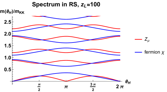
Figure 1: The mass spectrum of gauge fields $Z_{\mu}^{(n)}$ and fermion fields $\chi^{(n)}$ (type 1A) in the RS warped space is displayed. The warp factor is $z_{L}=100$ and the bulk mass parameter of $\Psi$ is $c=0.25$. There is no level crossing in the spectrum.

The KK expansion of the fermion field $\Psi$ in the twisted gauge in the region $1\leq z\leq z_{L}$ is expressed as

$$\begin{pmatrix}\tilde{\check{u}}_{R}(x,z)\cr\kern 5.0pt\cr\tilde{\check{d}}_{R}(x,z)\end{pmatrix} =\sqrt{k}\sum_{n=0}^{\infty}\chi_{R}^{(n)}(x)\,\tilde{\bf f}_{Rn}(z)~{},~{}\tilde{\bf f}_{Rn}(z)=\begin{pmatrix}\tilde{f}_{Rn}(z)\cr\tilde{g}_{Rn}(z)\end{pmatrix},$$ (2.39)

$$\begin{pmatrix}\tilde{\check{u}}_{L}(x,z)\cr\kern 5.0pt\cr\tilde{\check{d}}_{L}(x,z)\end{pmatrix} =\sqrt{k}\sum_{n=0}^{\infty}\chi_{L}^{(n)}(x)\,\tilde{\bf f}_{Ln}(z)~{},~{}\tilde{\bf f}_{Ln}(z)=\begin{pmatrix}\tilde{f}_{Ln}(z)\cr\tilde{g}_{Ln}(z)\end{pmatrix}.$$ (2.40)

The mode functions $\tilde{\bf f}_{Rn}(z)$ and $\tilde{\bf f}_{Ln}(z)$ for type 1A are given in (B.12). In the original gauge the expansions of $\check{u}(x,y)$ and $\check{d}(x,y)$ become

$$\begin{pmatrix}{\check{u}}_{R}(x,y)\cr\kern 2.0pt\cr{\check{d}}_{R}(x,y)\end{pmatrix} =\sqrt{k}\sum_{n=0}^{\infty}\chi_{R}^{(n)}(x)\begin{pmatrix}f_{Rn}(y)\cr g_{Rn}(y)\end{pmatrix},$$ (2.41)

$$\begin{pmatrix}{\check{u}}_{L}(x,y)\cr\kern 2.0pt\cr{\check{d}}_{L}(x,y)\end{pmatrix} =\sqrt{k}\sum_{n=0}^{\infty}\chi_{L}^{(n)}(x)\begin{pmatrix}f_{Ln}(y)\cr g_{Ln}(y)\end{pmatrix},$$ (2.42)

where

$$\underline{\hbox{type 1A}}~{}~{}$$ (2.43)

$$\begin{pmatrix}f_{Rn}(y)\cr g_{Rn}(y)\end{pmatrix} =\begin{pmatrix}f_{Rn}(-y)\cr-g_{Rn}(-y)\end{pmatrix}=\begin{pmatrix}f_{Rn}(y+2L)\cr g_{Rn}(y+2L)\end{pmatrix}$$ (2.44)

$$=\begin{pmatrix}\cos\hbox{$\frac{1}{2}$}\theta(z)&-\sin\hbox{$\frac{1}{2}$}\theta(z)\cr\kern 2.0pt\cr\sin\hbox{$\frac{1}{2}$}\theta(z)&\cos\hbox{$\frac{1}{2}$}\theta(z)\end{pmatrix}\begin{pmatrix}\tilde{f}_{Rn}(z)\cr\tilde{g}_{Rn}(z)\end{pmatrix}\quad{\rm for~{}}0\leq y\leq L~{},$$ (2.45)

$$\begin{pmatrix}f_{Ln}(y)\cr g_{Ln}(y)\end{pmatrix} =\begin{pmatrix}-f_{Ln}(-y)\cr g_{Ln}(-y)\end{pmatrix}=\begin{pmatrix}f_{Ln}(y+2L)\cr g_{Ln}(y+2L)\end{pmatrix}$$ (2.46)

$$=\begin{pmatrix}\cos\hbox{$\frac{1}{2}$}\theta(z)&-\sin\hbox{$\frac{1}{2}$}\theta(z)\cr\kern 2.0pt\cr\sin\hbox{$\frac{1}{2}$}\theta(z)&\cos\hbox{$\frac{1}{2}$}\theta(z)\end{pmatrix}\begin{pmatrix}\tilde{f}_{Ln}(z)\cr\tilde{g}_{Ln}(z)\end{pmatrix}\quad{\rm for~{}}0\leq y\leq L~{},$$ (2.47)

$$\underline{\hbox{type 2A}}~{}~{}$$ (2.48)

$$\begin{pmatrix}f_{Rn}(y)\cr g_{Rn}(y)\end{pmatrix} =\begin{pmatrix}f_{Rn}(-y)\cr-g_{Rn}(-y)\end{pmatrix}=\begin{pmatrix}-f_{Rn}(y+2L)\cr-g_{Rn}(y+2L)\end{pmatrix},$$ (2.49)

$$\begin{pmatrix}f_{Ln}(y)\cr g_{Ln}(y)\end{pmatrix} =\begin{pmatrix}-f_{Ln}(-y)\cr g_{Ln}(-y)\end{pmatrix}=\begin{pmatrix}-f_{Ln}(y+2L)\cr-g_{Ln}(y+2L)\end{pmatrix}.$$ (2.50)

For type 1B (2B), the parity of $f_{R/Ln},g_{R/Ln}$ is reversed compared to type 1A (2A).

3 Anomalies

Doublet fermions in type 1A or 1B are chiral at $\theta_{H}=0$. Massless modes appear for right-handed $u$ and left-handed $d$ (left-handed $u$ and right-handed $d$) for type 1A (1B). They become massive as $\theta_{H}$ varies, and their gauge couplings become purely vector-like at $\theta_{H}=\pi$. Chiral anomalies exist at $\theta_{H}=0$, smoothly vary as $\theta_{H}$ in the RS space, and vanish at $\theta_{H}=\pi$. This phenomenon is called the anomaly flow by an AB phase [12].

Chiral anomalies arise from triangular loop diagrams. Gauge couplings of fermions have been obtained in Ref.[12]. Substituting the KK expansions (2.35) and (2.42) into

$$g_{A}\int_{1}^{z_{L}}\frac{dz}{k}\,\Big{\{}{\check{\Psi}}_{R}^{\dagger}\bar{\sigma}^{\mu}A_{\mu}{\check{\Psi}}_{R}-{\check{\Psi}}_{L}^{\dagger}\sigma^{\mu}A_{\mu}{\check{\Psi}}_{L}\Big{\}}~{},$$ (3.1)

one finds that the couplings in

$$\frac{g_{4}}{2}\sum_{n=0}^{\infty}\sum_{\ell=0}^{\infty}\sum_{m=0}^{\infty}Z_{\mu}^{(n)}(x)\Big{\{}t^{R}_{n\ell m}\,\chi_{R}^{(\ell)}(x)^{\dagger}\bar{\sigma}^{\mu}\chi_{R}^{(m)}(x)+t^{L}_{n\ell m}\,\chi_{L}^{(\ell)}(x)^{\dagger}\sigma^{\mu}\chi_{L}^{(m)}(x)\Big{\}}$$ (3.2)

are given by

$$t^{R}_{n\ell m} =\int_{1}^{z_{L}}dz\,\Big{\{}\tilde{h}_{n}(z)\big{(}\tilde{f}_{R\ell}^{*}(z)\tilde{g}_{Rm}(z)+\tilde{g}_{R\ell}^{*}(z)\tilde{f}_{Rm}(z)\big{)}$$ (3.3)

$$\hskip 85.35826pt+\tilde{k}_{n}(z)\big{(}\tilde{f}_{R\ell}^{*}(z)\tilde{f}_{Rm}(z)-\tilde{g}_{R\ell}^{*}(z)\tilde{g}_{Rm}(z)\big{)}\Big{\}}$$ (3.4)

$$=\frac{k}{2}\int_{-a}^{2L-a}dy\,e^{\sigma(y)}\Big{\{}h_{n}(y)\big{(}f_{R\ell}^{*}(y)g_{Rm}(y)+g_{R\ell}^{*}(y)f_{Rm}(y)\big{)}$$ (3.5)

$$\hskip 85.35826pt+k_{n}(y)\big{(}f_{R\ell}^{*}(y)f_{Rm}(y)-g_{R\ell}^{*}(y)g_{Rm}(y)\big{)}\Big{\}},$$ (3.6)

$$t^{L}_{n\ell m} =-\int_{1}^{z_{L}}dz\,\Big{\{}h_{n}(z)\big{(}f_{L\ell}^{*}(z)g_{Lm}(z)+g_{L\ell}^{*}(z)f_{Lm}(z)\big{)}$$ (3.7)

$$\hskip 85.35826pt+k_{n}(z)\big{(}f_{L\ell}^{*}(z)f_{Lm}(z)-g_{L\ell}^{*}(z)g_{Lm}(z)\big{)}\Big{\}}$$ (3.8)

$$=-\frac{k}{2}\int_{-a}^{2L-a}dy\,e^{\sigma(y)}\Big{\{}h_{n}(y)\big{(}f_{L\ell}^{*}(y)g_{Lm}(y)+g_{L\ell}^{*}(y)f_{Lm}(y)\big{)}$$ (3.9)

$$\hskip 85.35826pt+k_{n}(y)\big{(}f_{L\ell}^{*}(y)f_{Lm}(y)-g_{L\ell}^{*}(y)g_{Lm}(y)\big{)}\Big{\}}.$$ (3.10)

The couplings $t^{R}_{n\ell m}$ and $t^{L}_{n\ell m}$ are gauge-invariant. In the integral formulas in the $y$-coordinate the constant $a$ is arbitrary as the integrands are periodic functions with period $2L$. It is convenient to take $0<a<L$ in the following discussions. We note that the couplings $t^{R/L}_{n\ell m}$ depend not only on $\theta_{H}$ and $z_{L}$, but also on the bulk mass parameter $c$ of the fermion field $\Psi$.

The anomaly coefficient associated with the three legs of $Z_{\mu_{1}}^{(n_{1})}Z_{\mu_{2}}^{(n_{2})}Z_{\mu_{3}}^{(n_{3})}$ is given by

$$a_{n_{1}n_{2}n_{3}}=a_{n_{1}n_{2}n_{3}}^{R}+a_{n_{1}n_{2}n_{3}}^{L}~{},$$ (3.11)

$$a_{n_{1}n_{2}n_{3}}^{R}={\rm Tr}\,T^{R}_{n_{1}}T^{R}_{n_{2}}T^{R}_{n_{3}}~{},~{}~{}(T^{R}_{n})_{m\ell}=t^{R}_{nm\ell}~{},$$ (3.12)

$$a_{n_{1}n_{2}n_{3}}^{L}={\rm Tr}\,T^{L}_{n_{1}}T^{L}_{n_{2}}T^{L}_{n_{3}}~{},~{}~{}(T^{L}_{n})_{m\ell}=t^{L}_{nm\ell}~{}.$$ (3.13)

The anomaly coefficient $a_{n_{1}n_{2}n_{3}}$ depends on $\theta_{H}$, exhibiting the anomaly flow. It has been observed by numerical evaluation in Ref.[12] that $a_{n_{1}n_{2}n_{3}}$ does not depend on the bulk mass parameter $c$, though $a_{n_{1}n_{2}n_{3}}^{R}$ and $a_{n_{1}n_{2}n_{3}}^{L}$ do depend on $c$. We are going to show that $a_{n_{1}n_{2}n_{3}}(\theta_{H},z_{L})$ is expressed in terms of the values of the wave functions $k_{n_{j}}(y)$ at $y=0$ and $y=L$.

To see it we insert the formulas for $t^{R/L}_{n\ell m}$ in (3.10) into (3.13), and rearrange the traces.

$$a_{n_{1}n_{2}n_{3}}=\Big{(}\frac{k}{2}\Big{)}^{3}\int\int\int_{-a}^{2L-a}dy_{1}dy_{2}dy_{3}\,e^{\sigma(y_{1})+\sigma(y_{2})+\sigma(y_{3})}$$ (3.14)

$$\quad\times\Big{[}~{}k_{1}k_{2}k_{3}\big{\{}A_{R}(1,2)A_{R}(2,3)A_{R}(3,1)-B_{R}(1,2)B_{R}(2,3)B_{R}(3,1)$$ (3.15)

$$\hskip 62.59596pt+B_{L}(1,2)B_{L}(2,3)B_{L}(3,1)-A_{L}(1,2)A_{L}(2,3)A_{L}(3,1)\big{\}}$$ (3.16)

$$\quad\quad+k_{1}h_{2}h_{3}\big{\{}A_{R}(1,2)B_{R}(2,3)A_{R}(3,1)-B_{R}(1,2)A_{R}(2,3)B_{R}(3,1)$$ (3.17)

$$\hskip 62.59596pt+B_{L}(1,2)A_{L}(2,3)B_{L}(3,1)-A_{L}(1,2)B_{L}(2,3)A_{L}(3,1)\big{\}}$$ (3.18)

$$\quad\quad+h_{1}k_{2}h_{3}\big{\{}A_{R}(1,2)A_{R}(2,3)B_{R}(3,1)-B_{R}(1,2)B_{R}(2,3)A_{R}(3,1)$$ (3.19)

$$\hskip 62.59596pt+B_{L}(1,2)B_{L}(2,3)A_{L}(3,1)-A_{L}(1,2)A_{L}(2,3)B_{L}(3,1)\big{\}}$$ (3.20)

$$\quad\quad+h_{1}h_{2}k_{3}\big{\{}B_{R}(1,2)A_{R}(2,3)A_{R}(3,1)-A_{R}(1,2)B_{R}(2,3)B_{R}(3,1)$$ (3.21)

$$\hskip 62.59596pt+A_{L}(1,2)B_{L}(2,3)B_{L}(3,1)-B_{L}(1,2)A_{L}(2,3)A_{L}(3,1)\big{\}}~{}\Big{]}$$ (3.22)

where

$$k_{j}=k_{n_{j}}(y_{j})~{},~{}~{}h_{j}=h_{n_{j}}(y_{j})~{},$$ (3.23)

$$\begin{pmatrix}A_{R/L}(j,k)\cr B_{R/L}(j,k)\end{pmatrix}=\begin{pmatrix}A_{R/L}\cr B_{R/L}\end{pmatrix}(y_{j},y_{k})=\sum_{n=0}^{\infty}\begin{pmatrix}f_{R/Ln}(y_{j})f_{R/Ln}^{*}(y_{k})\cr g_{R/Ln}(y_{j})g_{R/Ln}^{*}(y_{k})\end{pmatrix}.$$ (3.24)

Eqs. (2.40) and (2.42) and the orthonormality relations of the mode functions imply that

$$\begin{pmatrix}\check{u}_{R/L}(x,y)\cr\check{d}_{R/L}(x,y)\end{pmatrix}=\frac{k}{2}\int_{-a}^{2L-a}dy^{\prime}\,e^{\sigma(y^{\prime})}\begin{pmatrix}A_{R/L}&C_{R/L}\cr D_{R/L}&B_{R/L}\end{pmatrix}(y,y^{\prime})\begin{pmatrix}\check{u}_{R/L}(x,y^{\prime})\cr\check{d}_{R/L}(x,y^{\prime})\end{pmatrix},$$ (3.25)

$$\hskip 56.9055pt\begin{pmatrix}C_{R/L}\cr D_{R/L}\end{pmatrix}(y,y^{\prime})=\sum_{n=0}^{\infty}\begin{pmatrix}f_{R/Ln}(y)g_{R/Ln}^{*}(y^{\prime})\cr g_{R/Ln}(y)f_{R/Ln}^{*}(y^{\prime})\end{pmatrix}.$$ (3.26)

We have made use of the relation $C_{R/L}=D_{R/L}=0$ in deriving (3.22). With the choice of the AB phase $\theta_{H}$ in (2.28) all mode functions $\{f_{Rn}(y)\}$ etc. can be taken to be real so that $A_{R/L}(y,y^{\prime})=A_{R/L}(y^{\prime},y)$ and $B_{R/L}(y,y^{\prime})=B_{R/L}(y^{\prime},y)$.

In addition to the relation (3.26), $A_{R/L}$ and $B_{R/L}$ must satisfy the parity relations and boundary conditions of the mode functions. With $(y_{0},y_{1})=(0,L)$

$$\underline{\hbox{type 1A}}:$$ (3.27)

$$\begin{pmatrix}A_{R}\cr B_{R}\cr A_{L}\cr B_{L}\end{pmatrix}(y_{j}-y,y^{\prime})=\begin{pmatrix}A_{R}\cr-B_{R}\cr-A_{L}\cr B_{L}\end{pmatrix}(y_{j}+y,y^{\prime})~{},$$ (3.28)

$$\begin{pmatrix}\hat{D}_{-}(c)A_{R}(y,y^{\prime})\cr\hat{D}_{+}(c)B_{L}(y,y^{\prime})\end{pmatrix}_{y={\epsilon},L-{\epsilon}}=0~{},~{}\hat{D}_{\pm}(c)=\pm\frac{\partial}{\partial y}+c\,k~{},$$ (3.29)

$$B_{R}(y_{j},y^{\prime})=A_{L}(y_{j},y^{\prime})=0~{},$$ (3.30)

$$\underline{\hbox{type 2A}}:$$ (3.31)

$$\begin{pmatrix}A_{R}\cr B_{R}\cr A_{L}\cr B_{L}\end{pmatrix}(y_{j}-y,y^{\prime})=\begin{pmatrix}(-1)^{j}A_{R}\cr(-1)^{j+1}B_{R}\cr(-1)^{j+1}A_{L}\cr(-1)^{j}B_{L}\end{pmatrix}(y_{j}+y,y^{\prime})~{},$$ (3.32)

$$\begin{pmatrix}\hat{D}_{-}(c)A_{R}(y,y^{\prime})\cr\hat{D}_{+}(c)B_{L}(y,y^{\prime})\end{pmatrix}_{y={\epsilon}}=\begin{pmatrix}\hat{D}_{-}(c)B_{R}(y,y^{\prime})\cr\hat{D}_{+}(c)A_{L}(y,y^{\prime})\end{pmatrix}_{y=L-{\epsilon}}=0~{},$$ (3.33)

$$B_{R}(0,y^{\prime})=A_{R}(L,y^{\prime})=A_{L}(0,y^{\prime})=B_{L}(L,y^{\prime})=0~{}.$$ (3.34)

The condition for type 1B (2B) are obtained by interchanging $R$ (right-handed) and $L$ (left-handed) in those for type 1A (2A). For $c\not=0$, parity even components of $A_{R/L}$ and $B_{R/L}$ functions exhibit the cusp behavior at $y,y^{\prime}=0,\pm L,\cdots$.

It is not easy to explicitly write down $A_{R/L}(y,y^{\prime})$ and $B_{R/L}(y,y^{\prime})$ functions for $c\not=0$ which satisfy the relations in both (3.26) and (3.34). In the previous paper [12] it has been recognized that the anomaly coefficient $a_{n_{1}n_{2}n_{3}}$ in (3.22) is independent of $c$. With this observation we shall derive an analytical expression for $a_{n_{1}n_{2}n_{3}}$ by evaluating it in the case $c=0$. We will confirm later that numerically evaluated $a_{n_{1}n_{2}n_{3}}$ for $c\not=0$ agrees with the analytical formula.

Fermion wave functions for $c=0$ are expressed in terms of trigonometric functions. They are summarized in Appendix B.3. Inserting the wave functions in (B.24) into $A_{R}(z,z^{\prime})=\sum f_{Rn}(z)f_{Rn}^{*}(z^{\prime})$, for instance, one finds for type 1A that, for $1\leq z,z^{\prime}\leq z_{L}$,

$$A_{R}(z,z^{\prime})^{c=0}$$ (3.35)

$$=\frac{1}{z_{L}-1}\sum_{n=-\infty}^{\infty}\cos\Big{(}n\pi\frac{z-z_{L}}{z_{L}-1}+\alpha(z)\Big{)}\cos\Big{(}n\pi\frac{z^{\prime}-z_{L}}{z_{L}-1}+\alpha(z^{\prime})\Big{)}$$ (3.36)

$$=\delta_{2(z_{L}-1)}(z-z^{\prime})\cos\big{\{}\alpha(z)-\alpha(z^{\prime})\big{\}}+\delta_{2(z_{L}-1)}(z+z^{\prime}-2)\cos\big{\{}\alpha(z)+\alpha(z^{\prime})\big{\}}$$ (3.37)

$$=\delta_{2(z_{L}-1)}(z-z^{\prime})+\delta_{2(z_{L}-1)}(z+z^{\prime}-2)~{},$$ (3.38)

$$\quad\alpha(z)=\frac{1}{2}\Big{\{}\theta_{H}\,\frac{z-z_{L}}{z_{L}-1}+\theta(z)\Big{\}}~{},~{}\alpha(1)=\alpha(z_{L})=0~{}.$$ (3.39)

Here $\delta_{L}(x)=\sum_{n}\delta(x-nL)$. With the extension (2.50) in the $y$-coordinate and similar manipulation one finds that

$$\underline{\hbox{type 1A},~{}c=0}$$ (3.40)

$$A_{R}(y,y^{\prime})=B_{L}(y,y^{\prime})=\frac{e^{-\sigma(y)}}{k}\big{\{}\delta_{2L}(y-y^{\prime})+\delta_{2L}(y+y^{\prime})\big{\}}~{},$$ (3.41)

$$B_{R}(y,y^{\prime})=A_{L}(y,y^{\prime})=\frac{e^{-\sigma(y)}}{k}\big{\{}\delta_{2L}(y-y^{\prime})-\delta_{2L}(y+y^{\prime})\big{\}}~{},$$ (3.42)

Formulas for type 1B are obtained by interchanging $R$ and $L$.

For fermions in type 2A, one finds for $1\leq z,z^{\prime}\leq z_{L}$ that

$$A_{R}(z,z^{\prime})^{c=0}$$ (3.43)

$$=\frac{1}{z_{L}-1}\sum_{n=-\infty}^{\infty}\sin\Big{(}n\pi\frac{z-z_{L}}{z_{L}-1}+\beta(z)\Big{)}\sin\Big{(}n\pi\frac{z^{\prime}-z_{L}}{z_{L}-1}+\beta(z^{\prime})\Big{)}$$ (3.44)

$$=\delta_{2(z_{L}-1)}(z-z^{\prime})\cos\big{\{}\beta(z)-\beta(z^{\prime})\big{\}}-\delta_{2(z_{L}-1)}(z+z^{\prime}-2)\cos\big{\{}\beta(z)+\beta(z^{\prime})\big{\}}~{},$$ (3.45)

$$\quad\beta(z)=\frac{1}{2}\Big{\{}(\theta_{H}+\pi)\,\frac{z-z_{L}}{z_{L}-1}+\theta(z)\Big{\}}~{},~{}\beta(1)=-\frac{1}{2}\pi~{},~{}\beta(z_{L})=0~{}.$$ (3.46)

Noting the relations in (2.50), one finds in the $y$-coordinate that

$$\underline{\hbox{type 2A},~{}c=0}$$ (3.47)

$$A_{R}(y,y^{\prime})=B_{L}(y,y^{\prime})=\frac{e^{-\sigma(y)}}{k}\big{\{}\hat{\delta}_{2L}(y-y^{\prime})+\hat{\delta}_{2L}(y+y^{\prime})\big{\}}~{},$$ (3.48)

$$B_{R}(y,y^{\prime})=A_{L}(y,y^{\prime})=\frac{e^{-\sigma(y)}}{k}\big{\{}\hat{\delta}_{2L}(y-y^{\prime})-\hat{\delta}_{2L}(y+y^{\prime})\big{\}}~{},$$ (3.49)

$$\hat{\delta}_{2L}(y)=\delta_{4L}(y)-\delta_{4L}(y-2L)~{}.$$ (3.50)

Formulas for type 2B are obtained by interchanging $R$ and $L$.

We insert the expressions (3.42) or (3.50) into (3.22). There appear products of three delta functions in the integrand. Take $0<a<L$. Then in the integration range $-a\leq y_{1},y_{2},y_{3}\leq 2L-a$, products of delta functions reduce to

$$\begin{matrix}\delta_{2L}(y_{1}-y_{2})\delta_{2L}(y_{2}-y_{3})\delta_{2L}(y_{3}+y_{1})\cr\kern 5.0pt\cr\delta_{2L}(y_{1}+y_{2})\delta_{2L}(y_{2}+y_{3})\delta_{2L}(y_{3}+y_{1})\end{matrix}~{}\bigg{\}}$$ (3.51)

$$\quad\Rightarrow\frac{1}{2}\Big{\{}\delta(y_{1})\delta(y_{2})\delta(y_{3})+\delta(y_{1}-L)\delta(y_{2}-L)\delta(y_{3}-L)\Big{\}}~{},$$ (3.52)

$$\begin{matrix}\hat{\delta}_{2L}(y_{1}-y_{2})\hat{\delta}_{2L}(y_{2}-y_{3})\hat{\delta}_{2L}(y_{3}+y_{1})\cr\kern 5.0pt\cr\hat{\delta}_{2L}(y_{1}+y_{2})\hat{\delta}_{2L}(y_{2}+y_{3})\hat{\delta}_{2L}(y_{3}+y_{1})\end{matrix}~{}\bigg{\}}$$ (3.53)

$$\quad\Rightarrow\frac{1}{2}\Big{\{}\delta(y_{1})\delta(y_{2})\delta(y_{3})-\delta(y_{1}-L)\delta(y_{2}-L)\delta(y_{3}-L)\Big{\}}~{}.$$ (3.54)

As $h_{n}(0)=h_{n}(L)=0$, only the terms proportional to $k_{1}k_{2}k_{3}$ in (3.22) survive. We find the formula for the anomaly coefficients;

$$a_{n\ell m}(\theta_{H},z_{L}) =Q_{0}k_{n}(0)k_{\ell}(0)k_{m}(0)+Q_{1}k_{n}(L)k_{\ell}(L)k_{m}(L)~{},$$ (3.55)

$$(Q_{0},Q_{1}) =\begin{cases}(+1,+1)&\hbox{for type 1A}\cr(-1,-1)&\hbox{for type 1B}\cr(+1,-1)&\hbox{for type 2A}\cr(-1,+1)&\hbox{for type 2B}\end{cases}~{}.$$ (3.56)

The anomaly coefficients are determined by the values of the wave functions of the gauge fields at the UV and IR branes and the parity conditions of the fermion fields.

The formula (3.56) is strikingly simple. The wave function $k_{n}(y)$ depends on $\theta_{H}$ and $z_{L}$. The sum of the chiral anomalies arising from all possible fermion KK modes are summarized in terms of $k_{n}(0)$ and $k_{n}(L)$. The $c$-independence of those anomalies is confirmed numerically. The anomaly coefficients $a_{n\ell m}$ given by (3.56) are compared with those determined by first evaluating the gauge couplings $t^{R/L}_{n\ell m}$ ($0\leq\ell,m\leq\ell_{0}$) in (3.10) and then taking the traces of $(\ell_{0}+1)$-dimensional matrices in (3.13). In Figure 2 the results for $a_{000},a_{111},a_{222}$ and $a_{012}$ are shown for type 1A fermions with $c=0.25$, $\ell_{0}=10$ and $z_{L}=10$. One sees that the numerically evaluated values for $c=0.25$ fall on the universal curves given by (3.56). We have checked that the numerically evaluated values for other values of $c$ fall on the universal curves as well.

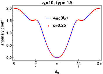
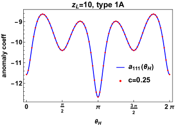
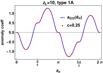
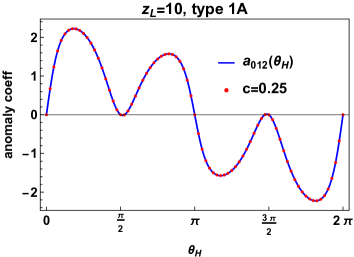
Figure 2: The anomaly coefficients $a_{000},a_{111},a_{222}$ and $a_{012}$ as functions of $\theta_{H}$ are shown for type 1A fermions for $z_{L}=10$. Blue curves represent the universal curves given by (3.56). Red dots represent the values determined from the gauge couplings $t^{R/L}_{n\ell m}$ ($0\leq\ell,m\leq\ell_{0}$) in (3.10) and then taking the traces of $(\ell_{0}+1)$-dimensional matrices in (3.13) for fermions with $c=0.25$ and $\ell_{0}=10$.

Some of $k_{n}(0;\theta_{H})$ and $k_{n}(L;\theta_{H})$ are plotted in Figure 3. Note that for $n=1,3,5,\cdots$, $|k_{n}(L;\theta_{H})|$ is much larger than $|k_{n}(0;\theta_{H})|$ for $z_{L}\geq 10$. Massless gauge bosons ($Z_{\mu}^{(0)}$) exist at $\theta_{H}=0$ and $\pi$. $k_{0}(0;0)=k_{0}(L;0)=1$ and $k_{0}(0;\pi)=-k_{0}(L;\pi)=1$ so that $a_{000}(\theta_{H}=0)=2$ and $a_{000}(\theta_{H}=\pi)=0$ for type 1A fermions and $a_{000}(\theta_{H}=0)=0$ and $a_{000}(\theta_{H}=\pi)=2$ for type 2A fermions. The anomaly flow is reflected in the behavior of the wave functions of the gauge fields at $y=0$ and $L$.

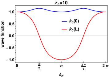
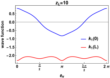
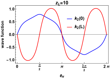
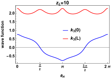
Figure 3: The values of the gauge wave functions $k_{n}(y;\theta_{H})$ ($n=0,1,2,3$) at $y=0$ (blue curves) and $y=L$ (red curves) for $z_{L}=10$ are shown.

Dependence of the anomaly coefficients $a_{n\ell m}$ on fermion types has a simple pattern. $a_{n\ell m}(\theta_{H})^{\rm{type}\,\rm{1A}}=-a_{n\ell m}(\theta_{H})^{\rm{type}\,\rm{1B}}$ and $a_{n\ell m}(\theta_{H})^{\rm{type}\,\rm{2A}}=-a_{n\ell m}(\theta_{H})^{\rm{type}\,\rm{2B}}$. Further $a_{n\ell m}(\theta_{H}+\pi)^{\rm{type}\,\rm{1A}}=a_{n\ell m}(\theta_{H})^{\rm{type}\,\rm{2A}}$ or $a_{n\ell m}(\theta_{H})^{\rm{type}\,\rm{2B}}$. (See Figure 4.) It follows from the property that $[k_{n}(0),k_{n}(L)]_{\theta_{H}+\pi}=[k_{n}(0),-k_{n}(L)]_{\theta_{H}}$ or $[-k_{n}(0),k_{n}(L)]_{\theta_{H}}$.

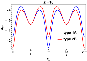
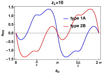
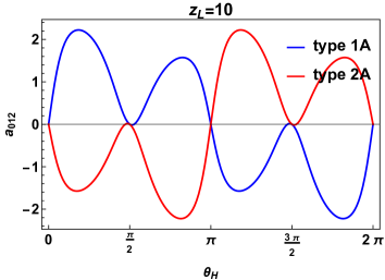
Figure 4: Dependence of the anomaly coefficients $a_{000},a_{111},a_{002}$ and $a_{012}$ on fermion types is shown for $z_{L}=10$. One sees that $a_{n\ell m}(\theta_{H}+\pi)^{\rm{type}\,\rm{1A}}=a_{n\ell m}(\theta_{H})^{\rm{type}\,\rm{2A}}$ or $a_{n\ell m}(\theta_{H})^{\rm{type}\,\rm{2B}}$.

Formulas in the flat $M^{4}\times(S^{1}/Z_{2})$ spacetime simplify. With the KK expansions (2.14), (2.19), and (2.21), the gauge couplings are written as

$$\frac{g_{4}}{2}\sum_{n=-\infty}^{\infty}\sum_{\ell=-\infty}^{\infty}\sum_{m=-\infty}^{\infty}B_{\mu}^{(n)}(x)\Big{\{}s^{R}_{n\ell m}\,\psi_{R}^{(\ell)}(x)^{\dagger}\bar{\sigma}^{\mu}\psi_{R}^{(m)}(x)+s^{L}_{n\ell m}\,\psi_{L}^{(\ell)}(x)^{\dagger}\sigma^{\mu}\psi_{L}^{(m)}(x)\Big{\}}$$ (3.57)

for type 1A and 1B fermions. For type 2A and 2B fermions $\psi_{R/L}^{(m)}(x)$ should be replaced by $\psi_{R/L}^{(m+\frac{1}{2})}(x)$. The anomaly coefficient associated with the three legs of $B_{\mu_{1}}^{(n_{1})}B_{\mu_{2}}^{(n_{2})}B_{\mu_{3}}^{(n_{3})}$ is given by

$$b_{n_{1}n_{2}n_{3}}=b_{n_{1}n_{2}n_{3}}^{R}+b_{n_{1}n_{2}n_{3}}^{L}~{},$$ (3.58)

$$b_{n_{1}n_{2}n_{3}}^{R}={\rm Tr}\,S^{R}_{n_{1}}S^{R}_{n_{2}}S^{R}_{n_{3}}~{},~{}~{}(S^{R}_{n})_{m\ell}=s^{R}_{nm\ell}~{},$$ (3.59)

$$b_{n_{1}n_{2}n_{3}}^{L}={\rm Tr}\,S^{L}_{n_{1}}S^{L}_{n_{2}}S^{L}_{n_{3}}~{},~{}~{}(S^{L}_{n})_{m\ell}=s^{L}_{nm\ell}~{}.$$ (3.60)

Applying the same argument as in the case of the RS space, one finds that

$$b_{n\ell m} =Q_{0}k^{\rm flat}_{n}(0)k^{\rm flat}_{\ell}(0)k^{\rm flat}_{m}(0)+Q_{1}k^{\rm flat}_{n}(L)k^{\rm flat}_{\ell}(L)k^{\rm flat}_{m}(L)$$ (3.61)

where $Q_{0},Q_{1}$ are given in (3.56). Since $k^{\rm flat}_{n}(y)=\cos(n\pi y/L)$ from (2.14), one finds that

$$b_{n\ell m} =Q_{0}+(-1)^{n+\ell+m}\,Q_{1}~{},$$ (3.62)

which agrees with the result in Ref.[12]. The formula (3.62) also results in the flat spacetime limit of (3.56). In the flat spacetime the level-crossing in the mass spectrum of gauge fields occurs at $\theta_{H}=0,\pm\hbox{$\frac{1}{2}$}\pi,\pm\pi,\cdots$. For this reason the flat spacetime limit of (3.56) becomes singular, as has been shown in Ref.[12].

4 Anomaly cancellation

The universality of the anomaly flow, expressed in the formula (3.56), has a profound implication in the model building, particularly in the GHU scenario. Chiral anomalies associated with gauge currents must be cancelled for the consistency of the theory in four dimensions [20, 21]. The fact that the anomaly coefficients are independent of the bulk mass parameters of fermions implies that anomaly cancellation can be achieved among various distinct fermions in the theory. In this section we examine this problem in the $SU(2)$ model.

Let us first recall the equations following from the action $I_{\rm RS}$ in (2.26) are, at the classical level,

$$\frac{1}{\sqrt{-\det G}}\,\partial_{M}\big{(}\sqrt{-\det G}\,F^{MN}\big{)}-ig_{A}[A_{M},F^{MN}]+J^{N}=0~{},$$ (4.1)

$${\cal D}(c)\,\Psi=0~{},$$ (4.2)

$$J^{N}=J^{Na}\frac{\tau^{a}}{2}~{},~{}~{}J^{Na}=-ig_{A}\overline{\Psi}\gamma^{A}{e_{A}}^{N}\frac{\tau^{a}}{2}\Psi~{}.$$ (4.3)

The current in five dimensions is covariantly conserved;

$$\frac{1}{\sqrt{-\det G}}\,\partial_{N}\big{(}\sqrt{-\det G}\,J^{N}\big{)}-ig_{A}[A_{N},J^{N}]=0~{}.$$ (4.4)

Note that the derivative term in the fifth coordinate generates mass terms in four dimensions when expanded in the KK modes. At the quantum level there arises an anomaly term on the righthand side of Eq. (4.4). The four-dimensional current $j_{(n)}^{\mu}(x)$ which couples with $Z_{\mu}^{(n)}(x)$ is

$$j_{(n)}^{\mu}(x) =\int_{0}^{L}dy\,\sqrt{-\det G}\,\big{\{}h_{n}(y)J^{\mu 1}+k_{n}(y)J^{\mu 3}\big{\}}$$ (4.5)

$$=\frac{g_{4}}{2}\sum_{\ell=0}^{\infty}\sum_{m=0}^{\infty}\Big{\{}t^{R}_{n\ell m}\,\chi_{R}^{(\ell)}(x)^{\dagger}\bar{\sigma}^{\mu}\chi_{R}^{(m)}(x)+t^{L}_{n\ell m}\,\chi_{L}^{(\ell)}(x)^{\dagger}\sigma^{\mu}\chi_{L}^{(m)}(x)\Big{\}}.$$ (4.6)

The divergence $\partial_{\mu}j_{(n)}^{\mu}$ picks up an anomalous term $j_{(n)}^{\rm anomaly}$ given by

$$j_{(n)}^{\rm anomaly}=-\Big{(}\frac{g_{4}}{2}\Big{)}^{3}\sum_{\ell=0}^{\infty}\sum_{m=0}^{\infty}\frac{a_{n\ell m}}{32\pi^{2}}\,{\epsilon}^{\mu\nu\rho\sigma}Z^{(\ell)}_{\mu\nu}Z^{(m)}_{\rho\sigma}$$ (4.7)

where $Z^{(\ell)}_{\mu\nu}=\partial_{\mu}Z_{\nu}^{(\ell)}-\partial_{\nu}Z_{\mu}^{(\ell)}$.

The conditions for the cancellation of the gauge anomalies are simple. Let the numbers of doublet fermions of type 1A, 1B, 2A and 2B be $n_{1A}$, $n_{1B}$, $n_{2A}$ and $n_{2B}$, respectively. It follows from (3.56) that the anomalies are cancelled if

$$n_{1A}=n_{1B}~{},~{}~{}n_{2A}=n_{2B}~{}.$$ (4.8)

In the presence of brane fermions, namely fermions living only on the UV or IR brane, the conditions are generalized. Suppose that there are $\hat{n}_{R}$ right-handed and $\hat{n}_{L}$ left-handed doublet brane fermions on the UV brane at $y=0$. As the $Z_{\mu}^{(n)}$ coupling of each brane fermion is given by $(g_{4}/2)\,k_{n}(0)$, the anomaly cancellation conditions become

$$n_{1A}-n_{1B}+n_{2A}-n_{2B}+\hat{n}_{R}-\hat{n}_{L}=0~{},$$ (4.9)

$$n_{1A}-n_{1B}-n_{2A}+n_{2B}=0~{},$$ (4.10)

We stress that the conditions (4.8) and (4.10) do not depend on $\theta_{H}$ and $z_{L}$. Furthermore the conditions guarantee that not only the zero mode anomaly $a_{000}$ but also all other anomalies $a_{n\ell m}$ are cancelled at once.

Fermion multiplets in the triplet representation do not contribute to anomalies in the $SU(2)$ gauge theory as is easily confirmed. The anomaly cancellation is achieved by the condition (4.8) or (4.10), namely by the condition for the numbers of doublet fermions with four types of orbifold boundary conditions. It does not depend on the AB phase $\theta_{H}$, namely the VEV of $A_{y}$. The situation is very similar to the anomaly cancellation condition in the SM.

5 Summary and discussions

In this paper we have examined the anomaly flow by the AB phase $\theta_{H}$ in the $SU(2)$ gauge theory in the RS space and in the flat $M^{4}\times(S^{1}/Z_{2})$ spacetime. The anomaly coefficients $a_{n\ell m}(\theta_{H},z_{L})$ induced by a fermion field in the bulk smoothly changes in $\theta_{H}$ in the RS space. Although the gauge couplings of the fermion, $t_{n\ell m}^{R/L}(\theta_{H},z_{L},c)$, nontrivially depend on the bulk mass parameter $c$ of the fermion, the total anomaly coefficients $a_{n\ell m}$ are independent of $c$. We have shown that those anomaly coefficients $a_{n\ell m}$ are expressed in terms of the values of the wave functions of the gauge fields at the UV and IR branes. The holographic formula (3.56) manifestly exhibits the $c$-independence. We have confirmed that the values of the anomaly coefficients numerically evaluated directly from $t_{n\ell m}^{R/L}(\theta_{H},z_{L},c)$ fall precisely on the curves given by (3.56). It has been left for future investigation to find an analytic proof of the $c$-independence of the expression (3.22).

As has been mentioned in the previous section, the universality in anomaly flow is critically important in the construction of realistic models of particle physics. GHU models have been proposed to unify the 4D Higgs boson with gauge fields in the framework of gauge theory on five-dimensional orbifolds in which the gauge hierarchy problem is naturally solved [5, 7, 22, 23, 24, 25, 26, 27, 28, 29, 30, 31, 32, 33, 34]. In particular, $SO(5)\times U(1)_{X}\times SU(3)_{C}$ GHU in the RS space with $\theta_{H}\sim 0.1$ and $z_{L}=10^{5}\sim 10^{10}$ has been shown to reproduce nearly the same phenomenology at low energies as the SM [31, 33]. As in the case of the SM, all chiral anomalies associated with gauge currents must be cancelled. Generalization of the argument on the universality to the group $SO(5)\times U(1)_{X}\times SU(3)_{C}$ is necessary. Further the technology developed in the present paper can be applied to the evaluation of anomalies of global currents such as baryon and lepton numbers. The phenomenon of anomaly flow may possibly be related to Chern-Simons terms in five dimensions[35, 36, 37]. These issues will be clarified in separate papers.

Appendix A Basis functions

Wave functions of gauge fields and fermions are expressed in terms of the following basis functions. For gauge fields we introduce

$$C(z;\lambda) =\frac{\pi}{2}\lambda zz_{L}F_{1,0}(\lambda z,\lambda z_{L})~{},$$ (A.1)

$$S(z;\lambda) =-\frac{\pi}{2}\lambda zF_{1,1}(\lambda z,\lambda z_{L})~{},$$ (A.2)

$$C^{\prime}(z;\lambda) =\frac{\pi}{2}\lambda^{2}zz_{L}F_{0,0}(\lambda z,\lambda z_{L})~{},$$ (A.3)

$$S^{\prime}(z;\lambda) =-\frac{\pi}{2}\lambda^{2}zF_{0,1}(\lambda z,\lambda z_{L})~{},$$ (A.4)

$$F_{\alpha,\beta}(u,v) \equiv J_{\alpha}(u)Y_{\beta}(v)-Y_{\alpha}(u)J_{\beta}(v)~{},$$ (A.5)

where $J_{\alpha}(u)$ and $Y_{\alpha}(u)$ are Bessel functions of the first and second kind. They satisfy

$$-z\frac{d}{dz}\frac{1}{z}\frac{d}{dz}\begin{pmatrix}C\cr S\end{pmatrix}=\lambda^{2}\begin{pmatrix}C\cr S\end{pmatrix}~{},$$ (A.6)

$$C(z_{L};\lambda)=z_{L}~{},~{}~{}C^{\prime}(z_{L};\lambda)=0~{},$$ (A.7)

$$S(z_{L};\lambda)=0~{},~{}~{}S^{\prime}(z_{L};\lambda)=\lambda~{},$$ (A.8)

$$CS^{\prime}-SC^{\prime}=\lambda z~{}.$$ (A.9)

To express wave functions of KK modes of gauge fields, we make use of

$$\hat{S}(z;\lambda)=N_{0}(\lambda)S(z;\lambda)~{},~{}~{}\hat{C}(z;\lambda)=N_{0}(\lambda)^{-1}C(z;\lambda)~{},$$ (A.10)

$$\check{S}(z;\lambda)=N_{1}(\lambda)S(z;\lambda)~{},~{}~{}\check{C}(z;\lambda)=N_{1}(\lambda)^{-1}C(z;\lambda)~{},$$ (A.11)

$$\qquad N_{0}(\lambda)=\frac{C(1;\lambda)}{S(1;\lambda)}~{},~{}~{}N_{1}(\lambda)=\frac{C^{\prime}(1;\lambda)}{S^{\prime}(1;\lambda)}~{}.$$ (A.12)

For fermion fields with a bulk mass parameter $c$, we define

$$\begin{pmatrix}C_{L}\cr S_{L}\end{pmatrix}(z;\lambda,c) =\pm\frac{\pi}{2}\lambda\sqrt{zz_{L}}F_{c+\frac{1}{2},c\mp\frac{1}{2}}(\lambda z,\lambda z_{L})~{},$$ (A.13)

$$\begin{pmatrix}C_{R}\cr S_{R}\end{pmatrix}(z;\lambda,c) =\mp\frac{\pi}{2}\lambda\sqrt{zz_{L}}F_{c-\frac{1}{2},c\pm\frac{1}{2}}(\lambda z,\lambda z_{L})~{}.$$ (A.14)

These functions satisfy

$$D_{+}(c)\begin{pmatrix}C_{L}\cr S_{L}\end{pmatrix}=\lambda\begin{pmatrix}S_{R}\cr C_{R}\end{pmatrix},$$ (A.15)

$$D_{-}(c)\begin{pmatrix}C_{R}\cr S_{R}\end{pmatrix}=\lambda\begin{pmatrix}S_{L}\cr C_{L}\end{pmatrix},~{}~{}D_{\pm}(c)=\pm\frac{d}{dz}+\frac{c}{z}~{},$$ (A.16)

$$C_{R}=C_{L}=1~{},~{}~{}S_{R}=S_{L}=0\quad{\rm at~{}}z=z_{L}~{},$$ (A.17)

$$C_{L}C_{R}-S_{L}S_{R}=1~{}.$$ (A.18)

Also $C_{L}(z;\lambda,-c)=C_{R}(z;\lambda,c)$ and $S_{L}(z;\lambda,-c)=-S_{R}(z;\lambda,c)$ hold. To express wave functions of KK modes of fermion fields, we make use of

$$\hat{S}_{L}(z;\lambda,c)=N_{L}(\lambda,c)S_{L}(z;\lambda,c)~{},~{}~{}\hat{C}_{L}(z;\lambda,c)=N_{R}(\lambda,c)C_{L}(z;\lambda,c)~{},$$ (A.19)

$$\hat{S}_{R}(z;\lambda,c)=N_{R}(\lambda,c)S_{R}(z;\lambda,c)~{},~{}~{}\hat{C}_{R}(z;\lambda,c)=N_{L}(\lambda,c)C_{R}(z;\lambda,c)~{},$$ (A.20)

$$\check{S}_{L}(z;\lambda,c)=N_{R}(\lambda,c)^{-1}S_{L}(z;\lambda,c)~{},~{}~{}\check{C}_{L}(z;\lambda,c)=N_{L}(\lambda,c)^{-1}C_{L}(z;\lambda,c)~{},$$ (A.21)

$$\check{S}_{R}(z;\lambda,c)=N_{L}(\lambda,c)^{-1}S_{R}(z;\lambda,c)~{},~{}~{}\check{C}_{R}(z;\lambda,c)=N_{R}(\lambda,c)^{-1}C_{R}(z;\lambda,c)~{},$$ (A.22)

$$\qquad N_{L}(\lambda,c)=\frac{C_{L}(1;\lambda,c)}{S_{L}(1;\lambda,c)}~{},~{}~{}N_{R}(\lambda,c)=\frac{C_{R}(1;\lambda,c)}{S_{R}(1;\lambda,c)}~{}.$$ (A.23)

Appendix B Wave functions in RS

B.1 Gauge fields $Z_{\mu}^{(n)}$

The mode functions of the gauge fields $Z_{\mu}^{(n)}(x)$ in (2.32) are given by

$$\tilde{\bf h}_{0}(z) =\bar{\bf h}_{0}^{a}(z)~{},$$ (B.1)

$$\tilde{\bf h}_{2\ell-1}(z) =(-1)^{\ell}\begin{cases}\bar{\bf h}_{2\ell-1}^{a}(z)&{\rm for}-\frac{1}{2}\pi<\theta_{H}<\frac{1}{2}\pi\cr\bar{\bf h}_{2\ell-1}^{b}(z)&{\rm for~{}}0<\theta_{H}<\pi\cr-\bar{\bf h}_{2\ell-1}^{a}(z)&{\rm for~{}}\frac{1}{2}\pi<\theta_{H}<\frac{3}{2}\pi\cr-\bar{\bf h}_{2\ell-1}^{b}(z)&{\rm for~{}}\pi<\theta_{H}<2\pi\cr\bar{\bf h}_{2\ell-1}^{a}(z)&{\rm for~{}}\frac{3}{2}\pi<\theta_{H}<\frac{5}{2}\pi\end{cases}~{}~{}(\ell=1,2,3,\cdots),$$ (B.2)

$$\tilde{\bf h}_{2\ell}(z) =(-1)^{\ell}\begin{cases}\bar{\bf h}_{2\ell}^{b}(z)&{\rm for}-\frac{1}{2}\pi<\theta_{H}<\frac{1}{2}\pi\cr-\bar{\bf h}_{2\ell}^{a}(z)&{\rm for~{}}0<\theta_{H}<\pi\cr-\bar{\bf h}_{2\ell}^{b}(z)&{\rm for~{}}\frac{1}{2}\pi<\theta_{H}<\frac{3}{2}\pi\cr\bar{\bf h}_{2\ell}^{a}(z)&{\rm for~{}}\pi<\theta_{H}<2\pi\cr\bar{\bf h}_{2\ell}^{b}(z)&{\rm for~{}}\frac{3}{2}\pi<\theta_{H}<\frac{5}{2}\pi\end{cases}~{}(\ell=1,2,3,\cdots),$$ (B.3)

$$\bar{\bf h}_{n}^{a}(z) =\frac{1}{\sqrt{r^{a}_{n}}}\begin{pmatrix}-s_{H}\hat{S}(z;\lambda_{n})\cr c_{H}C(z;\lambda_{n})\end{pmatrix},~{}~{}\bar{\bf h}_{n}^{b}(z)=\frac{1}{\sqrt{r^{b}_{n}}}\begin{pmatrix}c_{H}S(z;\lambda_{n})\cr s_{H}\check{C}(z;\lambda_{n})\end{pmatrix},$$ (B.4)

$$s_{H}=\sin\theta_{H}~{},~{}~{}c_{H}=\cos\theta_{H}~{},$$ (B.5)

$$r_{n}=\frac{1}{kL}\int_{1}^{z_{L}}\frac{dz}{z}\big{\{}|\hat{h}_{n}(z)|^{2}+|\hat{k}_{n}(z)|^{2}\big{\}}\quad{\rm for}~{}\begin{pmatrix}\hat{h}_{n}(z)\cr\hat{k}_{n}(z)\end{pmatrix}.$$ (B.6)

$\hat{S}$ and $\check{C}$ are given in (A.12). In the above formulas, the two expressions given in an overlapping $\theta_{H}$ region are the same. The connection formulas are necessary as one of them fails to make sense at the boundary in $\theta_{H}$.

B.2 Fermion fields $\chi_{R/L}^{(n)}$

The mode functions of the fermion fields $\chi_{R/L}^{(n)}(x)$ in (2.40) are given, for type 1A and $c>0$, by

$$\underline{\hbox{type 1A}}$$ (B.7)

$$\tilde{\bf f}_{R,2\ell}(z) =\begin{cases}\bar{\bf f}_{R,2\ell}^{a}(z)&{\rm for~{}}-\pi<\theta_{H}<\pi\cr\bar{\bf f}_{R,2\ell}^{b}(z)&{\rm for~{}}0<\theta_{H}<2\pi\cr-\bar{\bf f}_{R,2\ell}^{a}(z)&{\rm for~{}}\pi<\theta_{H}<3\pi\cr-\bar{\bf f}_{R,2\ell}^{b}(z)&{\rm for~{}}2\pi<\theta_{H}<4\pi\cr\bar{\bf f}_{R,2\ell}^{a}(z)&{\rm for~{}}3\pi<\theta_{H}<5\pi\cr\end{cases}~{}(\ell=0,1,2,\cdots),$$ (B.8)

$$\tilde{\bf f}_{R,2\ell-1}(z) =\begin{cases}\bar{\bf f}_{R,2\ell-1}^{c}(z)&{\rm for~{}}-\pi<\theta_{H}<\pi\cr\bar{\bf f}_{R,2\ell-1}^{d}(z)&{\rm for~{}}0<\theta_{H}<2\pi\cr-\bar{\bf f}_{R,2\ell-1}^{c}(z)&{\rm for~{}}\pi<\theta_{H}<3\pi\cr-\bar{\bf f}_{R,2\ell-1}^{d}(z)&{\rm for~{}}2\pi<\theta_{H}<4\pi\cr\bar{\bf f}_{R,2\ell-1}^{c}(z)&{\rm for~{}}3\pi<\theta_{H}<5\pi\cr\end{cases}~{}(\ell=1,2,3,\cdots),$$ (B.9)

$$\tilde{\bf f}_{L0}(z) =\bar{\bf f}_{L0}^{a}(z),$$ (B.10)

$$\tilde{\bf f}_{L,2\ell-1}(z) =\begin{cases}\bar{\bf f}_{L,2\ell-1}^{a}(z)&{\rm for~{}}-\pi<\theta_{H}<\pi\cr\bar{\bf f}_{L,2\ell-1}^{b}(z)&{\rm for~{}}0<\theta_{H}<2\pi\cr-\bar{\bf f}_{L,2\ell-1}^{a}(z)&{\rm for~{}}\pi<\theta_{H}<3\pi\cr-\bar{\bf f}_{L,2\ell-1}^{b}(z)&{\rm for~{}}2\pi<\theta_{H}<4\pi\cr\bar{\bf f}_{L,2\ell-1}^{a}(z)&{\rm for~{}}3\pi<\theta_{H}<5\pi\cr\end{cases}~{}(\ell=1,2,3,\cdots),$$ (B.11)

$$\tilde{\bf f}_{L,2\ell}(z) =\begin{cases}\bar{\bf f}_{L,2\ell}^{c}(z)&{\rm for~{}}-\pi<\theta_{H}<\pi\cr\bar{\bf f}_{L,2\ell}^{d}(z)&{\rm for~{}}0<\theta_{H}<2\pi\cr-\bar{\bf f}_{L,2\ell}^{c}(z)&{\rm for~{}}\pi<\theta_{H}<3\pi\cr-\bar{\bf f}_{L,2\ell}^{d}(z)&{\rm for~{}}2\pi<\theta_{H}<4\pi\cr\bar{\bf f}_{L,2\ell}^{c}(z)&{\rm for~{}}3\pi<\theta_{H}<5\pi\cr\end{cases}~{}(\ell=1,2,3,\cdots),$$ (B.12)

Here

$$\bar{\bf f}_{Rn}^{a}(z)=\frac{1}{\sqrt{r^{a}_{n}}}\begin{pmatrix}\bar{c}_{H}C_{R}(z;\lambda_{n},c)\cr-\bar{s}_{H}\hat{S}_{R}(z;\lambda_{n},c)\end{pmatrix},~{}~{}\bar{\bf f}_{Rn}^{b}(z)=\frac{1}{\sqrt{r^{b}_{n}}}\begin{pmatrix}\bar{s}_{H}C_{R}(z;\lambda_{n},c)\cr\bar{c}_{H}\check{S}_{R}(z;\lambda_{n},c)\end{pmatrix},$$ (B.13)

$$\bar{\bf f}_{Rn}^{c}(z)=\frac{1}{\sqrt{r^{c}_{n}}}\begin{pmatrix}\bar{s}_{H}\hat{C}_{R}(z;\lambda_{n},c)\cr\bar{c}_{H}S_{R}(z;\lambda_{n},c)\end{pmatrix},~{}~{}\bar{\bf f}_{Rn}^{d}(z)=\frac{1}{\sqrt{r^{d}_{n}}}\begin{pmatrix}-\bar{c}_{H}\check{C}_{R}(z;\lambda_{n},c)\cr\bar{s}_{H}S_{R}(z;\lambda_{n},c)\end{pmatrix},$$ (B.14)

$$\bar{\bf f}_{Ln}^{a}(z)=\frac{1}{\sqrt{r^{a}_{n}}}\begin{pmatrix}\bar{s}_{H}\hat{S}_{L}(z;\lambda_{n},c)\cr\bar{c}_{H}C_{L}(z;\lambda_{n},c)\end{pmatrix},~{}~{}\bar{\bf f}_{Ln}^{b}(z)=\frac{1}{\sqrt{r^{b}_{n}}}\begin{pmatrix}-\bar{c}_{H}\check{S}_{L}(z;\lambda_{n},c)\cr\bar{s}_{H}C_{L}(z;\lambda_{n},c)\end{pmatrix},$$ (B.15)

$$\bar{\bf f}_{Ln}^{c}(z)=\frac{1}{\sqrt{r^{c}_{n}}}\begin{pmatrix}\bar{c}_{H}S_{L}(z;\lambda_{n},c)\cr-\bar{s}_{H}\hat{C}_{L}(z;\lambda_{n},c)\end{pmatrix},~{}~{}\bar{\bf f}_{Ln}^{d}(z)=\frac{1}{\sqrt{r^{d}_{n}}}\begin{pmatrix}\bar{s}_{H}S_{L}(z;\lambda_{n},c)\cr\bar{c}_{H}\check{C}_{L}(z;\lambda_{n},c)\end{pmatrix},$$ (B.16)

$$\qquad\bar{c}_{H}=\cos\hbox{$\frac{1}{2}$}\theta_{H}~{},~{}\bar{s}_{H}=\sin\hbox{$\frac{1}{2}$}\theta_{H}~{},$$ (B.17)

$$\qquad r_{n}=\int_{1}^{z_{L}}dz\big{\{}|\hat{f}_{n}(z)|^{2}+|\hat{g}_{n}(z)|^{2}\big{\}}\quad{\rm for}~{}\begin{pmatrix}\hat{f}_{n}(z)\cr\hat{g}_{n}(z)\end{pmatrix}.$$ (B.18)

Functions $\hat{S}_{R/L},\check{S}_{R/L}$ etc. are defined in (A.23). In (B.12) two expressions in an overlapping region in $\theta_{H}$ are the same.

B.3 Fermion fields $\chi_{R/L}^{(n)}$ for $c=0$

For $c=0$ $C_{R/L}(z;\lambda,0)$ and $S_{R/L}(z;\lambda,0)$ reduce to trigonometric functions.

$$\begin{pmatrix}C_{L}\cr S_{L}\end{pmatrix}(z;\lambda,0) =\begin{pmatrix}\cos\lambda(z-z_{L})\cr\sin\lambda(z-z_{L})\end{pmatrix},$$ (B.19)

$$\begin{pmatrix}C_{R}\cr S_{R}\end{pmatrix}(z;\lambda,0) =\begin{pmatrix}\cos\lambda(z-z_{L})\cr-\sin\lambda(z-z_{L})\end{pmatrix}.$$ (B.20)

The spectrum and wave functions in $1\leq z=e^{ky}\leq z_{L}$ in the original gauge are given for type 1A by

$$\underline{\hbox{type 1A}}:$$ (B.21)

$$\lambda_{n}=\frac{1}{z_{L}-1}\big{|}n\pi+\hbox{$\frac{1}{2}$}\theta_{H}\big{|}\quad(-\infty<n<\infty),$$ (B.22)

$$\begin{pmatrix}f_{Rn}(y)\cr\kern 5.0pt\cr g_{Rn}(y)\end{pmatrix}=\frac{1}{\sqrt{z_{L}-1}}\begin{pmatrix}\cos\Big{\{}(n\pi+\hbox{$\frac{1}{2}$}\theta_{H})\frac{\displaystyle z-z_{L}}{\displaystyle z_{L}-1}+\hbox{$\frac{1}{2}$}\theta(z)\Big{\}}\cr\sin\Big{\{}(n\pi+\hbox{$\frac{1}{2}$}\theta_{H})\frac{\displaystyle z-z_{L}}{\displaystyle z_{L}-1}+\hbox{$\frac{1}{2}$}\theta(z)\Big{\}}\end{pmatrix},$$ (B.23)

$$\begin{pmatrix}f_{Ln}(y)\cr\kern 5.0pt\cr g_{Ln}(y)\end{pmatrix}=\frac{1}{\sqrt{z_{L}-1}}\begin{pmatrix}-\sin\Big{\{}(n\pi+\hbox{$\frac{1}{2}$}\theta_{H})\frac{\displaystyle z-z_{L}}{\displaystyle z_{L}-1}+\hbox{$\frac{1}{2}$}\theta(z)\Big{\}}\cr\cos\Big{\{}(n\pi+\hbox{$\frac{1}{2}$}\theta_{H})\frac{\displaystyle z-z_{L}}{\displaystyle z_{L}-1}+\hbox{$\frac{1}{2}$}\theta(z)\Big{\}}\end{pmatrix},$$ (B.24)

and for type 2A by

$$\underline{\hbox{type 2A}}:$$ (B.25)

$$\lambda_{n}=\frac{1}{z_{L}-1}\big{|}(n+\hbox{$\frac{1}{2}$})\pi+\hbox{$\frac{1}{2}$}\theta_{H}\big{|}\quad(-\infty<n<\infty),$$ (B.26)

$$\begin{pmatrix}f_{Rn}(y)\cr\kern 5.0pt\cr g_{Rn}(y)\end{pmatrix}=\frac{1}{\sqrt{z_{L}-1}}\begin{pmatrix}-\sin\Big{\{}(n\pi+\hbox{$\frac{1}{2}$}\pi+\hbox{$\frac{1}{2}$}\theta_{H})\frac{\displaystyle z-z_{L}}{\displaystyle z_{L}-1}+\hbox{$\frac{1}{2}$}\theta(z)\Big{\}}\cr\cos\Big{\{}(n\pi+\hbox{$\frac{1}{2}$}\pi+\hbox{$\frac{1}{2}$}\theta_{H})\frac{\displaystyle z-z_{L}}{\displaystyle z_{L}-1}+\hbox{$\frac{1}{2}$}\theta(z)\Big{\}}\end{pmatrix},$$ (B.27)

$$\begin{pmatrix}f_{Ln}(y)\cr\kern 5.0pt\cr g_{Ln}(y)\end{pmatrix}=\frac{1}{\sqrt{z_{L}-1}}\begin{pmatrix}\cos\Big{\{}(n\pi+\hbox{$\frac{1}{2}$}\pi+\hbox{$\frac{1}{2}$}\theta_{H})\frac{\displaystyle z-z_{L}}{\displaystyle z_{L}-1}+\hbox{$\frac{1}{2}$}\theta(z)\Big{\}}\cr\sin\Big{\{}(n\pi+\hbox{$\frac{1}{2}$}\pi+\hbox{$\frac{1}{2}$}\theta_{H})\frac{\displaystyle z-z_{L}}{\displaystyle z_{L}-1}+\hbox{$\frac{1}{2}$}\theta(z)\Big{\}}\end{pmatrix}.$$ (B.28)

Note that the expressions (B.24) and (B.28) reduce, up to normalization factors, to the expressions (2.19) and (2.21) in the flat spacetime limit, respectively. For other regions in $y$, the wave functions are defined by (2.50).

References

References

[1]
Y. Hosotani,
“Dynamical mass generation by compact extra dimensions”,
Phys. Lett. B126, 309 (1983).
[2]
A. T. Davies and A. McLachlan,
“Gauge group breaking by Wilson loops”,
Phys. Lett. B200, 305 (1988).
[3]
Y. Hosotani,
“Dynamics of nonintegrable phases and gauge symmetry breaking”,
Ann. Phys. (N.Y.)190, 233 (1989).
[4]
A. T. Davies and A. McLachlan,
“Congruency class effects in the Hosotani model”,
Nucl. Phys. B317, 237 (1989).
[5]
H. Hatanaka, T. Inami and C.S. Lim,
“The gauge hierarchy problem and higher dimensional gauge theories”,
Mod. Phys. Lett. A13, 2601 (1998).
[6]
H. Hatanaka,
“Matter representations and gauge symmetry breaking via compactified space”,
Prog. Theoret. Phys. 102, 407 (1999).
[7]
M. Kubo, C.S. Lim and H. Yamashita,
“The Hosotani mechanism in bulk gauge theories with an orbifold extra space ”,
Mod. Phys. Lett. A17, 2249 (2002).
[9]
J.S. Bell and R. Jackiw,
“A PCAC puzzle: in the model”,
Nuovo Cim. A60, 47 (1969).
[10]
K. Fujikawa,
“Path-integral measure for gauge-invariant fermion theories”,
Phys. Rev. Lett. 42, 1195 (1979).
[11]
K. Fujikawa,
“Path integral for gauge theories with fermions”,
Phys. Rev. D21, 2848 (1980).
[12]
S. Funatsu, H. Hatanaka, Y. Hosotani, Y. Orikasa and N. Yamatsu,
“Anomaly flow by an Aharonov-Bohm phase”,
Prog. Theoret. Exp. Phys. 2022, 043B04 (2022).
(arXiv:2202.01393)
[13]
S. Funatsu, H. Hatanaka, Y. Hosotani, Y. Orikasa and N. Yamatsu,
“Electroweak and left-right phase transitions in gauge-Higgs unification”,
Phys. Rev. D104, 115018 (2021).
[14]
C.G. Callan, Jr. and J.A. Harvey,
“Anomalies and fermion zero modes on strings and domail walls”,
Nucl. Phys. B250, 427 (1985).
[15]
H. Fukaya, T. Onogi and S. Yamaguchi,
“Atiyah-Patodi-Singer index from the domain-wall fermion Dirac operator”,
Phys. Rev. D96, 125004 (2017).
[16]
E. Witten and K. Yonekura,
“Anomaly inflow and the -invariant”,
arXiv:1909.08775.
[18]
Y. Hosotani and Y. Sakamura,
“Anomalous Higgs couplings in the gauge-Higgs unification in warped spacetime”,
Prog. Theoret. Phys. 118, 935 (2007).
[19]
L. Randall and R. Sundrum,
“A large mass hierarchy from a small extra dimension”,
Phys. Rev. Lett. 83, 3370 (1999).
[20]
C. Bouchiat, J. Iliopoulos and Ph. Meyer,
“An anomaly-free version of Weinberg’s model”,
Phys. Lett. B38, 519 (1972).
[21]
D.J. Gross and R. Jackiw,
“Effects of anomalies on quasi-renormalizable theories”,
Phys. Rev. D6, 477 (1972).
[22]
G. Burdman and Y. Nomura,
“Unification of Higgs and gauge fields in five dimensions”,
Nucl. Phys. B656, 3 (2003).
[23]
C. Csaki, C. Grojean and H. Murayama,
“Standard model Higgs from higher dimensional gauge fields”,
Phys. Rev. D67, 085012 (2003).
[24]
C.A. Scrucca, M. Serone, L. Silvestrini,
“Electroweak symmetry breaking and fermion masses from extra dimensions”,
Nucl. Phys. B669, 128 (2003).
[25]
K. Agashe, R. Contino and A. Pomarol,
“The minimal composite Higgs model”,
Nucl. Phys. B719, 165 (2005).
[26]
G. Cacciapaglia, C. Csaki, S.C. Park,
“Fully radiative electroweak symmetry breaking”,
JHEP03, 099 (2006).
[27]
A. D. Medina, N. R. Shah and C. E. M. Wagner,
“Gauge-Higgs unification and radiative electroweak symmetry breaking in warped extra dimensions”,
Phys. Rev. D76, 095010 (2007).
[28]
Y. Hosotani, K. Oda, T. Ohnuma and Y. Sakamura,
“Dynamical electroweak symmetry breaking in gauge-Higgs
unification with top and bottom quarks”,
Phys. Rev. D78, 096002 (2008);
Erratum-ibid. D79, 079902 (2009).
[29]
Y. Hosotani, S. Noda and N. Uekusa,
“The electroweak gauge couplings in gauge-Higgs unification”,
Prog. Theoret. Phys. 123, 757 (2010).
[30]
S. Funatsu, H. Hatanaka, Y. Hosotani, Y. Orikasa and T. Shimotani,
“Novel universality and Higgs decay in the gauge-Higgs unification”,
Phys. Lett. B722, 94 (2013).
[31]
S. Funatsu, H. Hatanaka, Y. Hosotani, Y. Orikasa and N. Yamatsu,
“GUT inspired gauge-Higgs unification”,
Phys. Rev. D99, 095010 (2019).
[32]
J. Yoon and M.E. Peskin,
“Dissection of an gauge-Higgs unification model”,
Phys. Rev. D100, 015001 (2019).
[33]
S. Funatsu, H. Hatanaka, Y. Hosotani, Y. Orikasa and N. Yamatsu,
“CKM matrix and FCNC suppression in gauge-Higgs unification”,
Phys. Rev. D101, 055016 (2020).
[34]
S. Funatsu, H. Hatanaka, Y. Hosotani, Y. Orikasa and N. Yamatsu,
“Fermion pair production at linear collider experiments
in GUT inspired gauge-Higgs unification”,
Phys. Rev. D102, 015029 (2020);
[35]
B. Gripaios and S.M. West,
“Anomaly holography”,
Nucl. Phys. B789, 362 (2008).
[36]
S. Hong and G. Rigo,
“Anomaly inflow and holography”,
JHEP05, 72 (2021).
[37]
Y. Adachi, C.S. Lim, and N. Maru,
“The strong CP problem and higher dimensional gauge theories”,
arXiv:2108.07367.