An intuition for physicists: information gain from experiments

Abstract

How much one has learned from an experiment is quantifiable by the information gain, also known as the Kullback-Leibler divergence. The narrowing of the posterior parameter distribution $P(\theta|D)$ compared with the prior parameter distribution $\pi$($\theta$), is quantified in units of bits, as:

$$D_{\mathrm{KL}}(P|\pi)=\int\log_{2}\left(\frac{P(\theta|D)}{\pi(\theta)}\right)\,P(\theta|D)\,d\theta$$

This research note gives an intuition what one bit of information gain means. It corresponds to a Gaussian shrinking its standard deviation by a factor of three.

1 Gaussian update

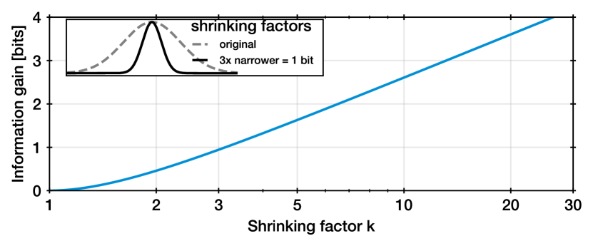
Figure 1: The more the Gaussian shrinks (x-axis), the higher the information gain (y-axis, in bits). The inset illustrates a shrinkage factor $k=3$ between prior (dashed) and posterior (solid curve).

Consider for the posterior a Gaussian with standard deviation $\sigma$, and for the prior a Gaussian at the same mean, but wider by a factor $k$, $\sigma^{\prime}=k\sigma$. The inset of Figure 1 illustrates this scenario. After some computation we find:

$$D_{\mathrm{KL}} =\int\left(2\pi\sigma{{}^{2}}\right)^{-\frac{1}{2}}e^{-\frac{\theta{{}^{2}}}{2\sigma^{2}}}\times\left(-\frac{1}{2}\log_{2}\left(2\pi\sigma{{}^{2}}\right)-\frac{\theta{{}^{2}}}{2\sigma^{2}}+\frac{1}{2}\log_{2}\left(2\pi\sigma{{}^{2}}k^{2}\right)+\frac{\theta{{}^{2}}}{2\sigma^{2}k^{2}}\right)d\theta$$

$$=\log_{2}k+\left(k^{-2}-1\right)/2/\ln 2$$

This relation between the more intuitive “Gaussian shrinkage factor $k$” and bits is illustrated in Figure 1.

The update of a flat prior distribution to a flat posterior distribution narrowed by a shrinkage factor $k$ gives $D_{\mathrm{KL}}(P|\pi)=\log_{2}k$. That is, two (eight) bits corresponds to $k=4$ ($256$). This follows the usual computer science interpretation that removing $b$ bits restricting the possibility space by a factor of $2^{b}$, which here is the shrinkage factor of the posterior volume $k$.

2 Estimation from posterior samples

The information gain can be computed easily from one-dimensional histograms of posterior samples as:

$$D_{\mathrm{KL}}(P|\pi)\approx\sum_{i}\frac{n_{i}}{N}\log_{2}\frac{n_{i}/N}{m_{i}/M},$$

where $n_{i}$ ($m_{i}$) are posterior (prior) samples within bin $i$, out of $N$ ($M$) total samples. If the bin widths are sized to contain equal prior mass (e.g., equal size for uniform priors), the formula simplifies to: $D_{\mathrm{KL}}(P|\pi)\approx\sum_{i=1}^{B}n_{i}/N\log_{2}\left(n_{i}B/N\right)$. Empty bins should be skipped. Negative $D_{\mathrm{KL}}$ are numerical artifacts and should be set to zero.

The general-purpose Bayesian inference package UltraNest (Buchner, 2021) computes the information gain overall (using the method of Skilling, 2004) and for each parameter.

References

• Buchner (2021) Buchner, J. 2021, The Journal of Open Source Software, 6, 3001
• Skilling (2004) Skilling, J. 2004, AIP Conference Proceedings, 735, 395