Optically detected magnetic resonance with an open source platform

Abstract

Localized electronic spins in solid-state environments form versatile and robust platforms for quantum sensing, metrology and quantum information processing. With optically detected magnetic resonance (ODMR), it is possible to prepare and readout highly coherent spin systems, up to room temperature, with orders of magnitude enhanced sensitivities and spatial resolutions compared to induction-based techniques, allowing for single spin manipulations. While ODMR was first observed in organic molecules, many other systems have since then been identified. Among them is the nitrogen-vacancy (NV) center in diamond, which is used both as a nanoscale quantum sensor for external fields and as a spin qubit. Other systems permitting ODMR are rare earth ions used as quantum memories and many other color centers trapped in bulk or 2-dimensional host materials. In order to allow the broadest possible community of researchers and engineers to investigate and develop novel ODMR-based materials and applications, we review here the setting up of ODMR experiments using commercially available hardware. We also present in detail the dedicated collaborative open-source interface named Qudi and describe the features we added to speed-up data acquisition, relax instrument requirements and extend its applicability to ensemble measurements. Covering both hardware and software development, this article aims to overview the setting of ODMR experiments and provide an efficient, portable and collaborative interface to implement innovative experiments to optimize the development time of ODMR experiments for scientists of any backgrounds.

Introduction

Spin is a quantum property of elementary particles which confers them an intrinsic magnetic moment that can be associated with a circulating charge flow in their wave function Ohanian (1998). In atoms and ions, while the nuclear spins remain essentially shielded, the unpaired electrons result in magnetic moments that are three order of magnitude stronger – of the order of the Bohr magneton. It makes electron spins the main contributors to most materials’ magnetic properties. In the modern context of the second quantum revolution Dowling and Milburn (2003), electron spins, such as in quantum dots Vandersypen et al. (2017); Zhang et al. (2018a), color centers in diamond Chang, Hsiao, and Su (2018) or silicon carbide Castelletto and Boretti (2020), or rare earth ions Bertaina et al. (2007) have been either studied as individual quantum systems or as ensembles. While electron spins naturally interact with various external and internal fields, they can also be isolated from unwanted perturbations by experimental design or choice of system Camenzind et al. (2018), making them either great quantum sensors Degen, Reinhard, and Cappellaro (2017) or highly coherent quantum bits (or qubits) for quantum information processing Wesenberg et al. (2009); Pezzagna and Meijer (2021).

Standard inductive radio- and microwave techniques for spin resonance measurements suffer from poor sensitivity and low spatial resolution. Indeed, under achievable magnetic fields electronic spin transition energies typically lie in the microwave (MW) domain, with associated Boltzmann temperatures of few tens of millikelvin, so that they are very weakly polarized at ambient conditions. Additionally, sensing MW fields at the single photon level remains a tremendous challenge Lescanne et al. (2020) and the associated wavelengths (millimeter to centimeter) is by far larger than the few tens of nanometers required for directly probing spin-spin interactions Dolde et al. (2014). Even using magnetic field gradients magnetic resonance imaging (MRI) cannot achieve spatial resolution below tens of micrometers Blank et al. (2009). All these limitations affect both the spatial resolution in quantum sensing and the scaling of entangled qubits’ networks for useful quantum computing.

Optically detected magnetic resonance (ODRM) Suter (2020) offers a powerful solution to these problems. It is applicable to a range of material systems (see Table 1) whose joint optical and magnetic properties render their electron-spin magnetic transition detectable in the optical domain. The following ingredients are characteristics of ODMR systems:

• Firstly, the electronic spin can be polarized by optical pumping to a much higher degree than under thermal equilibrium. Associated with naturally low spin-lattice coupling Gugler et al. (2018), certain electronic spins can maintain long polarization and coherence times even at elevated temperature Balasubramanian et al. (2009). Together these properties can totally relax the need for cryogenic conditions.

• Secondly, the strength of optical signal (typically absorption, fluorescence or phosphorescence) must depend on the electronic spin state or its projection along a quantization axis. Since optical fields can routinely be detected at the shot-noise limit, the sensitivity of magnetic resonance spectroscopy and the fidelity of spin state readout can be significantly increased while spin initialization and readout can be achieved with a much higher spatial resolution set by the optical wavelength (or below).

• Finally, these advantages can be translated to nuclear spin spectroscopy through the use of hyperfine coupling Nishimura et al. (2020).

Together, these features are placing ODMR at the core of many emerging spin-based quantum technologies.

Despite the growing number of researchers and engineers active in this area and the availability of advanced optical and microwave (MW) equipment, building and operating an ODMR setup for a specific purpose usually demands substantial hardware and software developments. Moreover, beyond the apparent simplicity of ODMR measurements, a certain amount of tacit knowledge is needed to avoid some pitfalls that can spoil measurement accuracy and reproducibility.

The object of this article is twofold: (i) to describe a typical ODMR setup, from its conception and construction to the optimization of specific measurements and (ii) to present, in details, the ODMR-dedicated open source platform Qudi Binder et al. (2017) with the features we developed for speeding-up acquisitions, relaxing instrumental requirements, widening its applications and lowering entry barriers.

In Sec. I, we first recall ODMR main principles and measurement techniques and review the most studied material systems with their applications. We then present the hardware configuration needed for ODMR experiments in Sec. II. Aspects related to optical setup, generation of MW signals, pulses and bias magnetic fields are discussed. We show how some ODMR experiments (in continuous wave and pulsed modes) can be visualized directly with an oscilloscope and determine when the use of a computer interface is useful or required. In Sec. III, we describe how these instruments are connected together and present the most common strategies for synchronizing ODMR experiments. Both the computer and oscilloscope interfaces are covered. The section IV is dedicated to the open source platform Qudi, first release in 2017 Binder et al. (2017) and upgraded by us for efficient and versatile ODMR experiment operations. Finally, in Sec. V we give a few practical advice to perform reliable and contrasted measurements, in particular accounting for technical noise and instrument imperfections. We take a specific focus on NV center ensembles as an illustrative scenario.

We believe that the software experimental developments presented here will help newcomers achieve faster and better results for their desired application and provide experts an efficient, portable, and collaborative platform to explore innovative experiments.

I Optically Detected Magnetic Resonance

I.1 Main principles

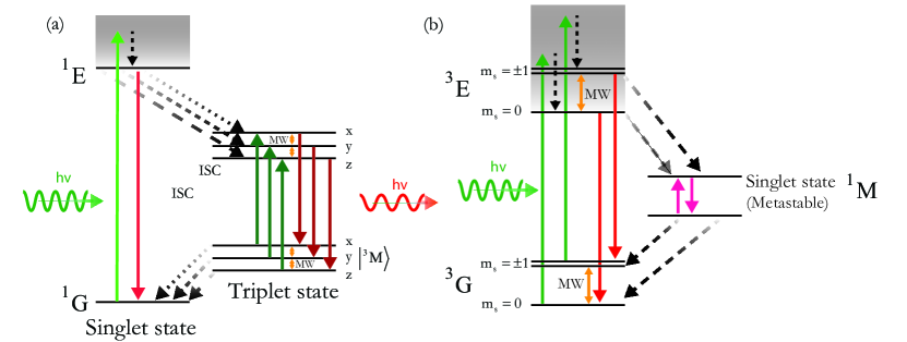
Figure 1: InterSystem Crossing (ISC) based ODMR dynamics when the ground state is singlet (a) or triplet (b).

ODMR relies on two main features: (i) initialization (i.e. polarization) of the spin state under optical excitation (spin pumping) and (ii) spin-state-dependent optical properties, such as fluorescence, phosphorescence, absorption, or, as more recently demonstrated, photocurrent Bourgeois, Gulka, and Nesladek (2020), used for spin state readout. While feature (i) boosts the contrast of the spin resonance signal, feature (ii) allows to advantageously trade low energy MW photons for much higher energy optical ones in the spin state measurement. These properties may arise from spin-orbit coupling (see Fig. 1), a relativistic effect that allows for inter-system crossing (ISC), e.g. transitions between singlet $S=0$ and triplet $S=1$ state manifolds Penfold et al. (2018); Marian (2012) (in a spin-1 system). The probability of ISC may depend on the initial spin state, which in turn may result in spin-dependent optical properties and spin-dependent relaxation pathways. In other systems (see Sec. I.3), ODMR can be achieved under resonant optical pumping such as using $\Lambda$-shaped configurations.

I.2 Interactions with external quantities

In a system that is not isotropic, a quantization axis emerges; noting $m_{S}$ the spin quantum number (i.e. the spin projection along that axis), the dipolar spin-spin interaction lifts the degeneracy between the states $\left|m_{S}=0\right>$ and $\left|m_{S}=\pm 1\right>$ among the $S=1$ triplet, by an amount called zero-field splitting (ZFS), often denoted with $D$. Further degeneracy is lifted between $\left|m_{S}=-1\right>$ and $\left|m_{S}=+1\right>$ by a parameter $E$ when the symmetry is less than axial. The eigenstates, potentially made of superpositions of pure spin states, are then often denoted $x$, $y$ and $z$. $D$ and $E$ depend on geometrical aspects and therefore on pressure and temperature. In addition, Stark and Zeeman effects further separate the $\left|m_{S}=-1\right>$ and $\left|m_{S}=+1\right>$ state which makes ODMR systems naturally sensitive to magnetic and electric fields. Finally, further interactions may occur with other electron or nuclear spins, resulting in more level splittings, spin dephasing and diffusion, etc.

I.3 Main ODMR systems and their applications

We can distinguish two main configurations linked to the multiplicity of the ground state (see Fig. 1). The ground state of organic molecules are typically spin singlets, where all electrons are paired in covalent bonds or lone pairs Carbonera (2009). Photoexcitation followed by ISC may promote the molecule into a spin triplet state and enable ODMR as in Fig. 1 (a). Since 1967 Kwiram, Alvin L. (1967); Schmidt et al. (1967); Sharnoff (2004), such process has been exploited to enhance the detection limit of magnetic resonance Carbonera (2009) with a particular application in photosynthesis research Giacometti et al. (2007); Kwiram and Ross (1982). ODMR from a single molecule was reported for the first time in 1993 independently by Wrachtrup et al. Wrachtrup et al. (1993) and Köhler et al. Köhler et al. (1993). Both experiments relied on the photoexcited metastable triplet state of a pentacene molecule trapped in a p-terphenyl host crystal. Pentacene’s spin-dependent optical properties have also been used inside MW resonators Arroo, Alford, and Breeze (2021), such as for demonstrating the first room temperature maser Oxborrow, Breeze, and Alford (2012) or conversely for cooling a microwave mode Wu et al. (2021).

The negatively charged Nitrogen-Vacancy center (NV^-) in diamond - hereafter called NV center - belongs to the second configuration depicted in Fig. 1 (b). Its ground ³A₂ and main excited ³E optical states are spin triplets. The first single NV center ODMR signal was reported by Gruber et al. in 1997 Gruber et al. (1997). For the following reasons, NV centers then became the most studied ODMR system:

• ISC combined with a low Debye-Waller factor allows for an efficient off-resonance optical pumping and readout over a large range of wavelengths, even far over room temperature Liu et al. (2019) and under high pressures Doherty et al. (2014).

• Diamond is bio-compatible making NV-doped nanodiamonds particularly relevant Chipaux et al. (2018) when used as biomarkers Haziza et al. (2017); Hemelaar et al. (2017); Miller et al. (2020) or quantum sensors Sigaeva et al. (2022a); Morita et al. (2023); Zhang et al. (2021).

• NV centers can exhibit long spin relaxation and coherence times Balasubramanian et al. (2009) thanks to the low density of nuclear spins in diamond and the decoupling of spin states from lattice phonons Gugler et al. (2018). It makes them versatile quantum sensors Barry et al. (2020) for detection and imaging of magnetic and electric fields, temperature, strain, currents and associated noises Degen, Reinhard, and Cappellaro (2017); Schirhagl et al. (2014); Rondin et al. (2014), as well as for microwave field imaging Shao et al. (2016) or spectroscopy Chipaux et al. (2015a); Meinel et al. (2021).

• NV center ODMR properties can be extended to polarize Healey et al. (2021); Rizzato et al. (2022); Gao et al. (2022) and/or detect Mamin, Sherwood, and Rugar (2012); Staudacher et al. (2013); Sushkov et al. (2014); Lovchinsky et al. (2016) other electron or nuclear spins in their vicinity and perform their magnetic resonance spectroscopyWood et al. (2016); Mignon et al. (2023). In these cases the sensitivity can go down to a single nuclear spin, orders of magnitude better than conventional electron paramagnetic resonance (EPR) and nuclear magnetic resonance (NMR) methods.

• Finally, thanks to their excellent coherence properties and couplings to even longer lived nuclear spins Bradley et al. (2019), NV centers are also promising qubits for quantum information processing Pezzagna and Meijer (2021) and fundamental studies of quantum mechanics Hensen et al. (2015).

Other diamond defects from the group IV-vacancy category Bradac et al. (2019) have recently revealed their ODMR signals, such as the negatively charged silicon-vacancy center (SiV^-) Pingault et al. (2017) and its neutral form (SiV⁰) Zhang et al. (2020), the Germanium-Vacancy (GeV) Siyushev et al. (2017) and the Tin-Vacancy (SnV) Iwasaki et al. (2017) centers. In these cases, ODMR is possible only at cryogenic temperatures since it requires resonant optical addressing – differing from the scheme presented in Fig. 1. Single-defect ODMR signals have recently been reported in silicon carbide Nagy et al. (2018); Castelletto and Boretti (2020); Yan et al. (2020) or hexagonal boron nitride Stern et al. (2022); Murzakhanov et al. (2022). Notably, the so called V1 center in silicon carbide Nagy et al. (2018) involves a spin quartet $S=\frac{3}{2}$ ground state. Rare earth ions in crystal lattices are also intensely studied for long lasting and broadband optical quantum memories Zhong and Goldner (2019); Grimm et al. (2021). One can cite $Ce^{3+}$ in YAG Xia et al. (2015) or $Yb^{3+}$ Zhou et al. (2020) and $Eu^{3+}$ Ortu et al. (2022) in $Y_{2}SiO_{5}$. Semiconductor quantum dots have also been used in ODMR experiments Ivanov et al. (2018); O. Tolmachev et al. (2020). The optical wavelengths and microwave frequencies associated to those systems are summarized in Table 1.

System	Optical pumping	Microwave	Comments / Applications
(host)	[Off-resonance]	Zero field splitting $D\textrm{ and }E$
	(On-resonance (ZPL))	Gyromagnetic ratio $\gamma$
Organic molecules	Various	$D=500\textrm{ to }$1500\text{\,}\mathrm{MHz}$$	Sensitive EPR spectroscopy Carbonera (2009)
		$E=0\textrm{ to }$500\text{\,}\mathrm{MHz}$$	Photosynthesis Agostini et al. (2021)
Pentacene	[Green - yellow,	$D=$1395\text{\,}\mathrm{MHz}$$	First single molecule ODMR signal Wrachtrup et al. (1993); Köhler et al. (1993)
(p-terphenyl crystal)	e.g. $585\text{\,}\mathrm{nm}$]	$E=$53\text{\,}\mathrm{MHz}$$	First room temperature maser Oxborrow, Breeze, and Alford (2012); Arroo, Alford, and Breeze (2021)
NV- center	[Green e.g. $515\textrm{ or }$532\text{\,}\mathrm{n}\mathrm{m}$$]	$D=$2.87\text{\,}\mathrm{GHz}$$	Quantum sensing
(Diamond)	$($637\text{\,}\mathrm{n}\mathrm{m}$=$1.945\text{\,}\mathrm{eV}$)$	$\gamma=$28\text{\,}\mathrm{GHz}\text{\,}{\mathrm{T}}^{-1}$$	Quantum computation
Group IV-Vacancy			Cryogenic temperature. Becker and Neu (2020)
centers (Diamond)			Quantum networks Chen, Zheludev, and Gao (2020)
SiV-	$($737\text{\,}\mathrm{nm}$)$	$D=$50\text{\,}\mathrm{GHz}$$	Pingault et al. (2017)
SiV0	$($946\text{\,}\mathrm{nm}$)$	$D=$944\text{\,}\mathrm{GHz}$$	Zhang et al. (2020)
GeV	$($612\text{\,}\mathrm{nm}$)$	$D=$170\text{\,}\mathrm{GHz}$$	Siyushev et al. (2017)
SnV	$($260\text{\,}\mathrm{nm}$)$		Iwasaki et al. (2017)
V1 center	$\left($861\text{\,}\mathrm{nm}$\right)$	$D=$2\text{\,}\mathrm{MHz}$$	Spin quartet Nagy et al. (2018)
PL8 center	[$920\text{\,}\mathrm{nm}$]	$D=$1.39\text{\,}\mathrm{GHz}$$	Room temperature Yan et al. (2020)
(4H-Silicon carbide)	$\left(1007\textrm{ to }$1024\text{\,}\mathrm{nm}$\right)$	$E=$4\text{\,}\mathrm{MHz}$$	Castelletto and Boretti (2020)
Unknown defects	[$532\text{\,}\mathrm{nm}$]	$D=0.1\textrm{ to }$2.4\text{\,}\mathrm{GHz}$$	Stern et al. (2022)
(Boron Nitride)
Rare earth ions			Quantum memories Zhong and Goldner (2019); Grimm et al. (2021)
$Ce^{3+}$ (YAG)	$\left(460\textrm{ and }$486\text{\,}\mathrm{nm}$\right)$	$<2$2.2\text{\,}\mathrm{GHz}$$	Xia et al. (2015)
$Yb^{3+}$ ($Y_{2}SiO_{5}$)	$\left($980\text{\,}\mathrm{nm}$\right)$	$<$2.62\text{\,}\mathrm{GHz}$$	Zhou et al. (2020)
$Eu^{3+}$ ($Y_{2}SiO_{5}$)	$\left($580\text{\,}\mathrm{nm}$\right)$	$34.5$ and $46.2\text{\,}\mathrm{MHz}$	Ortu et al. (2022)
Quantum dots
(In,Al)As/(AlAs)	[$360\textrm{ and }$404\text{\,}\mathrm{nm}$]$		Ivanov et al. (2018)
CdSe/(Cd,Mn)S	[$405\text{\,}\mathrm{nm}$]	$60\text{\,}\mathrm{GHz}$	O. Tolmachev et al. (2020)

Table 1: Summary of some popular ODMR systems and their main parameters.

I.4 Main ODMR techniques

I.4.1 Continuous wave mode

ODMR can be performed under continuous wave (CW) optical and MW excitation. A CW-ODMR spectrum is obtained by recording the optical emission or absorption as function of the MW frequency that is being swept. When spin resonances are reached, dips or peaks appear in the recorded optical intensity (see Fig. 2), allowing to measure physical parameters affecting the resonance frequencies or to determine the gyromagnetic ratio of the system itself (EPR spectroscopy). For a given system, several external parameters affect the precision of the spectrum obtained by CW-ODMR through the change in signal-to-noise ratio and spin resonance linewidth. These parameters include MW power (via power broadening Dréau et al. (2011) and sample heating), laser power (via change in excitation rate, governing spin polarization, optical emission and photo-ionization rates), MW sweeping method and pace, etc. Optimization of CW-ODMR signal acquisition is discussed in Sec. V.2.

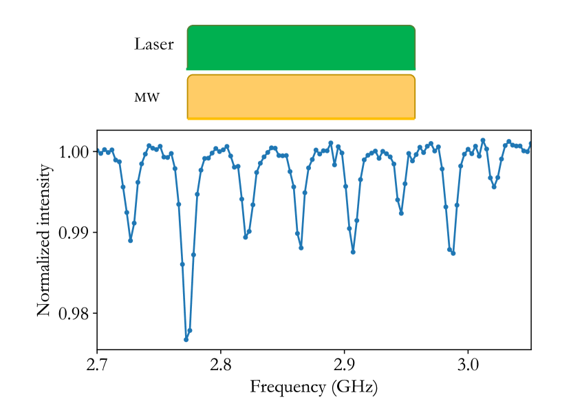
Figure 2: Example of a continuous-wave ODMR spectrum from an NV-center ensemble under d.c. magnetic field, displaying eight resonances (hyperfine splitting not resolved) with contrasts on the order of 1%.

I.4.2 Pulse sequences

Pulsed ODMR has the first advantage of mitigating power broadening by letting the system evolve freely after optical and MW excitation. It also allows to tune the system for being specifically sensitive to certain quantities and insensitive to unwanted perturbations, taking advantage of decades of development in the field of magnetic resonance spectroscopy Vandersypen and Chuang (2005). Good practices for optimizing a pulsed ODMR signal are discussed in Sec. V.3. Below, we first introduce the most elementary pulse sequences (in the case of a spin triplet).

Common to most sequences, a first laser pulse initializes the system (e.g. in state $|m_{S}=0\rangle$). After a period of spin manipulation with MW pulses and/or free evolution, a second laser pulse interrogates the spin state projection along the $\left(|m_{S}=0\rangle,|m_{S}=+1\rangle\right)$ basis through the optical emission or absorption intensity. It also re-initializes the system for the subsequent measurement. In the Bloch sphere representation, a MW $\pi$-pulse performs a $\pi$ rotation along a certain axis; for instance, it can swap the $|m_{S}=0\rangle$ and $|m_{S}=+1\rangle$ (or $|m_{S}=-1\rangle$). A $\pi/2$ pulse only performs a quarter turn, placing an initial $|m_{S}=0\rangle$ state into an equal superposition $\frac{1}{\sqrt{2}}\left(|m_{S}=0\rangle+e^{i\phi}|m_{S}=+1\rangle\right)$ (or $|-1\rangle$).

Relaxometry – $T_{1}$ measurement

— This sequence, reported in Fig. 3(a), requires no MW fields. The two initialization and readout optical pulses are separated by a varying dark time $\tau$. It allows for probing the relaxation dynamics from an initialized pure state to a thermal equilibrium. Interesting for applications, the relaxation time, or $T_{1}$, can sense the magnetic noise of the local environment Tetienne et al. (2013); Rollo et al. (2021) such as the one created by free radicals species in living cells Sigaeva et al. (2022a); Morita et al. (2023) or by chemical reactions Barton et al. (2020).

Rabi sequence – $\pi$-pulse calibration

— In this sequence, reported in Fig. 3(b), the delay between the optical pulses is fixed and a MW pulse is applied for a varying duration $\tau$ (alternatively, its power can be varied). The measured optical signal as a function of $\tau$ shows Rabi oscillations. From this measurement the duration of $\pi$ and $\frac{\pi}{2}$-pulses can be inferred as half and quarter periods of the oscillations, respectively.

Ramsey sequence – $T_{2}^{*}$ measurement

— This sequence, reported in Fig. 3(c), consists in a pump-probe experiment where two $\pi/2$ pulses are inserted. The first $\pi/2$, immediately after the initialization laser pulse, induces spin precession. After the free evolution time $\tau$ the precession is halted by a second $\pi/2$ pulse before the read-out laser pulse is applied. The optical signal as function of $\tau$ presents oscillations at the difference-frequency between the applied MW field and the spin transition being probed. Therefore, this sequence can be used for d.c. sensing and offers better sensitivity compared to the CW-ODMR approach Dréau et al. (2011) by eluding the detrimental effect of power broadening. Ramsey fringes are damped with a time constant reflecting the spin dephasing time or heterogeneous decoherence time called $T_{2}^{*}$.

Hahn echo sequence – $T_{2}$ measurement

— This sequence, reported in Fig. 3(d), uses a $\pi$-pulse in the middle of the Ramsey sequence. This approach mitigates the effect of slowly fluctuating fields (such as from the nuclear spin bath) by canceling in the second half of the evolution the accumulated phase difference from the first half and restoring the original coherence. The characteristic decay time measured with this protocol is usually called $T_{2}$, and can typically be one or two orders of magnitude longer than $T_{2}^{*}$. More and more complex and faster dynamical decoupling sequences can be employed to extend $T_{2}$; yet, it remains bounded by relaxation time through $T_{2}<2\cdot T_{1}$. Such echo sequence is particularly suitable of a.c. field sensing as it can filter a narrow frequency window Degen, Reinhard, and Cappellaro (2017).

Many efforts have been devoted to develop and optimize pulse sequences for increasing sensitivities to specific quantities and frequencies while canceling other noises. A comprehensive review dedicated to NV centers can be found in Barry et al. (2020).

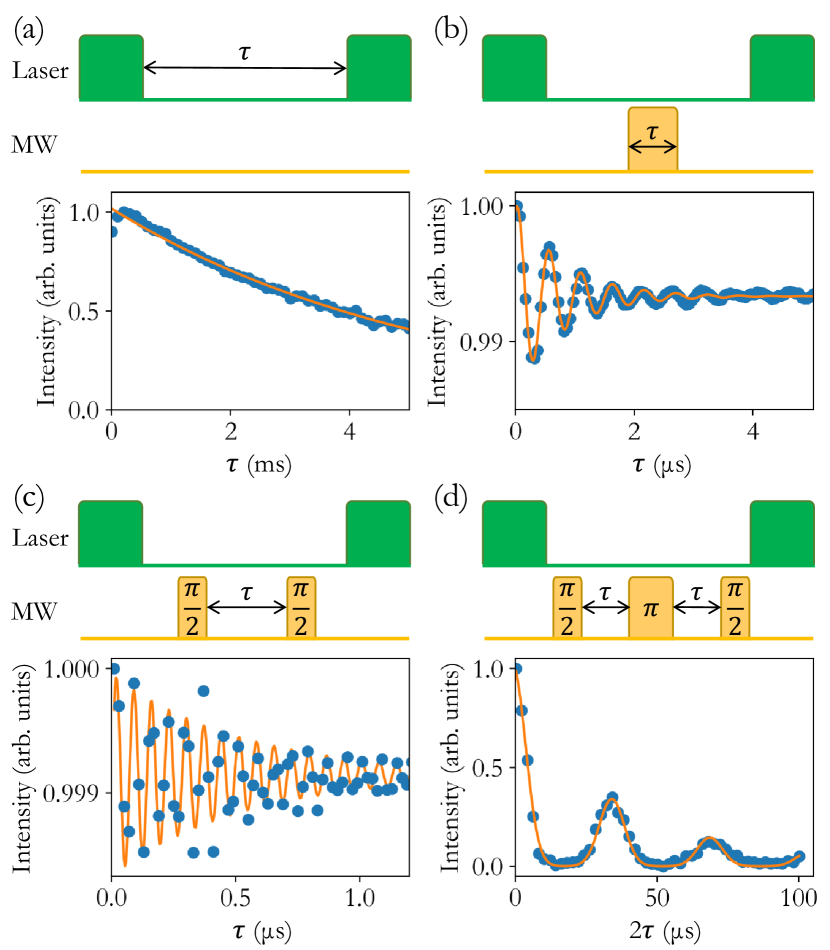
Figure 3: Most common pulse sequences for ODMR: a) Relaxometry b) Rabi sequence c) Ramsey sequence d) Hahn echo sequence. In each panel, laser and MW pulses are represented schematically in the top part. In the bottom part, NV centers’ experimental data obtained in our set-up from are shown.

II Hardware for continuous and pulsed ODMR

We review here the instrumental requirements for ODMR measurements in terms of optical setup, MW generation and biased magnetic field. Both CW and pulsed ODMR measurements are discussed. We take the diamond NV center as an accessible example (green pumping, red photoluminescence (PL)). However, the properties of other defects summarized in Table 1 can be consulted in order to adapt the equipment for their study, with a special care given on the optical wavelengths, microwave frequencies and possible need for cryogenic environment.

II.1 Photoluminescence microscopy

As mentioned in Sec. I, ODMR relies on monitoring an optical signal such as the PL. It is obtained by directing a pumping beam (a laser or LED) onto the system of interest and routing the luminescence signal onto a photodectector (such as an amplified photodiode, a single photon counting module or a camera).

The simple optical setup reported in Fig. 4 analogous to an epifluorescence microscope can represent the minimal required optical setup to perform ODMR. An excitation laser beam is reflected on a dichroic mirror and focused on the sample via a microscope objective or a simple lens. The sample’s luminescence is collected by the same lens and sent to a photodetector. Alternatively, the sample can be pumped from another side or by total internal reflection Chipaux et al. (2015b); Wolf et al. (2015); Clevenson et al. (2015) to relax the need for a dichroic mirror or optimize pump power utilization and spatial homogeneity of excitation. An inverted configuration of the microscope (e.g. where the objective is below the sample) is preferred when using liquid immersion objectives, especially for biological applications Webb et al. (2021).

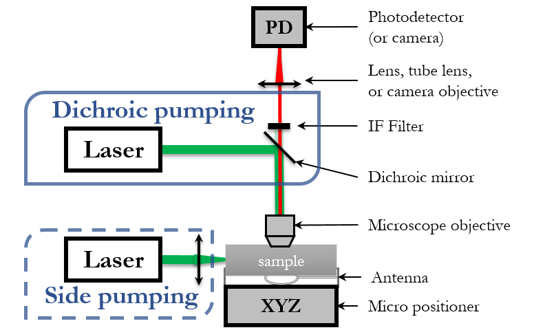
Figure 4: Schematic of a simple OMDR setup.

II.1.1 Light detector and imaging mode

The choice of the light detector is probably the most impacting point in the development of a new setup. It is governed by two main aspects:

Single-pixel vs. wide-field imaging

— In the former case, a photodetector is sufficient, with appropriate filters placed in front of it to discriminate the signal of interest from the scattered laser light and the possible background luminescence from ODMR-inactive centers Jonkman et al. (2020). At the cost of small loss of transmitted power, spatially filtering the luminescence signal through a confocal pinhole or an optical fiber reduces the out-of-focus background and collection area (see Fig. 5). If imaging capability is desired it can be obtained by confocal scanning (see II.1.5 and Fig. 5).

For wide-field imaging, a pixel array (camera) is required in combination with a large and homogeneous illumination area. Comprehensive reviews about wide-field imaging in the particular case of NV centers can be found in Levine et al. (2019); Nomura (2021); Scholten et al. (2021). Besides, accordingly to the specific experiments, different cameras (e.g. CCD or a CMOS) can be preferred Wojciechowski et al. (2018).

Strength of optical signal

— It depends on the number of luminescent centers or molecules being addressed, their individual quantum yields and the collection + detection efficiency. For the study of single or few emitters, a digital photon counter (d-PC) is necessary, such as a reverse-biased avalanche photodiode operated in Geiger mode or a superconducting nanowire detector. d-PCs generate electrical pulses (e.g. TTL) upon photon absorption with a quantum efficiency that can exceed 80%, allowing for the study of photon fluxes down to sub-kHz level, limited by the dark count rate of the detector.

For measurements on large ensembles, d-PCs typically saturate at count rates of few tens of MHz (i.e. few picowatts at visible wavelengths). Above that analog photodectors (a-PDs) can be used, such as amplified or avalanche photodiodes. In a wide-field configuration with a weakly emitting system, particularly sensitive cameras are required such as Electron Multiplying CCD (low noise) or phosphorus intensified camera (gated).

To enhance the sensitivity in under significant background signal, one can modulate and demodulate the ODMR signal (e.g. through the applied MW frequency) with the help of a lock-in amplifier Kuwahata et al. (2020). Such methods can be of great help in the context of biosensing where background emission is strong Miller et al. (2020). For wide-field imaging, the recently developed arrays for lock-in detector Wojciechowski et al. (2018) may find numerous applications in the upcoming years.

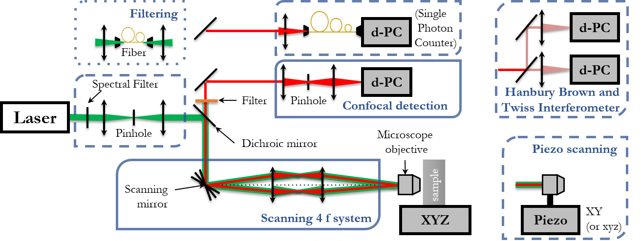
Figure 5: Schematic of a typical home-build confocal microscope used for low light ODMR experiments. The collimated laser beam is spectrally filtered (to remove broadband spontaneous emission) before being reflected on the dichroic mirror and focused on the sample using a high-NA objective lens. Photoluminescence is collected by the same objective, passes through the dichroic mirror and an interference filter (band-pass or long-pass) to reject the excitation light, and is optionally spatially filtered using a confocal pinhole or an optical fiber before its intensity is measured by the detector. In order to scan the sample both a scanning mirror or a piezo stage can be used. To study single emitters, a Hanbury-Brown and Twiss interferometer can be added.

II.1.2 Optical components and alignment

When addressing individual emitters, one of the most important parameters is the objective’s numerical aperture ($NA$) defined as $NA=n\,\sin{\theta}$, with $n$ the refractive index of the immersion medium and ${\theta}$ the half-cone angle of collection. For isotropic emission pattern, it limits the fraction of collected to emitted light to:

$$\eta<\frac{1}{2}\left(1-\cos{\theta}\right)$$ (1)

with $\cos{\theta}={\sqrt{1-{(NA/n)}^{2}}}$.

Through diffraction, it also limits the achievable resolution $r_{min}$ defined as the minimum distance at which two objects can be distinguished. As commonly determined by the Rayleigh criterion:

$$r_{min}=\frac{r_{Airy}}{2}=0.61\cdot\frac{\lambda}{NA}$$ (2)

where $\lambda$ is the wavelength of the optical source and $r_{Airy}$ the radius of its diffraction pattern on the sample. Similarly, the axial (depth) resolution is set by:

$$z_{min}=1.4\frac{\lambda n}{{NA}^{2}}$$ (3)

A larger $NA$ is usually obtained at the cost of a smaller working distance. As a good compromise, an air objective with $NA$ up to 0.9 can offer a working distance of 1 mm. In contrast, in a confocal setting, the magnification $M_{obj}$ of the microscope objective bears no direct relation to spatial resolution and collection efficiency. It matters however for the design of the excitation and collection optics as well as in the case of wide-field imaging on a pixel array.

To achieve a spatial resolution limited by Abbe's diffraction and avoid unnecessary light loss, care should be taken to the following aspects:

• Firstly, the excitation beam diameter $\Phi$ should match or exceed the back aperture diameter of the microscope objective given by:

  $$\Phi=2f^{\prime}_{obj}\tan{\theta}$$ (4)

  with $\tan{\theta}=\frac{NA/n}{\sqrt{1-{(NA/n)}^{2}}}$, $f^{\prime}_{obj}=\frac{l_{tube}}{M_{obj}}$ the effective focal lens of the microscope objective, $l_{tube}$ being the tube lens as defined by the microscope supplier (e.g. $180\text{\,}\mathrm{m}\mathrm{m}$ for Olympus, $200\text{\,}\mathrm{m}\mathrm{m}$ for Nikon and Mitutoyo and $165\text{\,}\mathrm{m}\mathrm{m}$ for Zeiss).

• Secondly, the confocal pinhole of radius $r_{hole}$ (or optical fiber of numerical aperture $NA_{fiber}$) has to be chosen to match the diffraction pattern of the photoluminescence beam on the pinhole (or fiber). When the image is sent to infinity after the objective the total magnification up to the pinhole (or fiber) equals:

  $$M_{tot}=M_{obj}*M_{lens}=M_{obj}\frac{f^{\prime}_{lens}}{l_{tube}}$$ (5)

  where $f^{\prime}_{lens}$ is the focal length of the lens used to focus on the pinhole. So to provide good confocal resolution while avoiding significant optical loss, $r_{hole}$ can be chosen to match the radius of the Airy diffraction pattern:

  $$r_{hole}=1.22\times M_{tot}\frac{\lambda_{PL}}{NA}$$ (6)

  Here, $\lambda_{PL}$ refers to the wavelength of the photoluminescent signal. The pinhole can also be chosen smaller. This would enhance the resolution (e.g. reduce $r_{min}$) by a factor down to $2/3$, at the cost of more optical loss.

• If an optical fiber is used instead, its numerical aperture can be taken as:

  $$NA_{fiber}=\frac{NA}{M_{tot}}$$ (7)

  In those cases, either the focusing lens, the pinhole or optical fiber can be changed to obtain the desired spatial filtering. Further details about the basics of confocal microscopy can be found in Jerome and Price (2018).

Many efforts have been devoted to surpass the diffraction limit in ODMR using super-resolution techniques such as stochastic optical reconstruction microscopy (STORM) and stimulated emission depletion (STED) microscopy Hsiao et al. (2016); Jin et al. (2018).

II.1.3 Light source

For the most studied ODMR systems (Sec. I.3), the optical pumping can be performed off resonance. Consequently, there is no stringent requirement on temporal coherence and linewidth of the light source, so that even a white-light LED can be employed, as long as suitable filter sets are used to prevent leakage of excitation light into the detector. However, fluctuations in laser power affects the contrast of the ODMR, as well as the stability and coherence of the NV centers. Therefore, it is important to carefully control the laser power fluctuation against temperature.

Transverse spatial coherence (single mode emission) is required in a confocal configuration in order to obtain a diffraction-limited spot size at the focus. As shown in Fig. 5, a spatial filter (pinhole or mono-mode fiber) can be introduced in the excitation path to improve transverse coherence. In this case, and using large NA, optical powers of milliwatts or less are often sufficient to saturate the emitter. Therefore, commercially available solid state lasers are a great and affordable option. Optionally, neutral density filters allow to adjust the power incident on the sample while maintaining the laser at its optimal operating power. In the wide-field configuration, the laser power is diluted over the entire area of interest, requiring high power lasers up to watts level. In all cases, temporal fluctuation in laser power represents the main source of technical noise, which can be mitigated by adding a feedback control loop or monitoring laser power in real time through a second detector. Other forms of technical noises related to pulsed measurements are discussed in Sec. II.3.

II.1.4 PL digitization and visualization

Different approaches are used to measure the PL as a function of the type of signal coming from the photodetector.

Analog photodetectors (a-PDs) deliver an electric signal proportional to light intensity (temporally averaged over a given bandwidth) that can be visualized directly on an oscilloscope for both continuous and pulsed measurements. Alternatively, a computer interfaced acquisition card that embeds an Analog to Digital Converter (ADC) can be used. In this context, the most relevant features of these data acquisition cards (DAQ) are the number of input and output channels and the maximum sampling rate. The sampling rate sets an upper limit to the fastest dynamics that can be measured under analog acquisition. While the oscilloscope sampling rate can be chosen up to the GHz range, the DAQ analog inputs are often limited to a few MHz. Modern oscilloscopes can be interfaced on a computer for direct collection of the data temporally stored in the oscilloscope (see Sec. IV.1). In case of pulsed acquisition (see Sec. II.3) averaging over several repetition is needed to obtain sufficient signal to noise ratio and/or to reduce the communication bandwidth requirement with the computer. Consequently, it demands a sync pulse for each repetition and limits the averaging strategy to the $NP$ method described in Sec. III.4.

Digital photocounters (d-PCs) deliver nanosecond pulses (e.g. TTL) with sharp rising edge. In such case, the use of a computer becomes almost unavoidable. Conventionally, a time tagging instrument or counter (e.g. from Swabian instruments or PicoQuant) provides time resolution down to picosecond range, below the typical timing jitter of the detector. Such resolution can be useful to resolve the PL lifetime (see Sec. V), or to acquire second order autocorrelation function $(g^{(2)})$ (e.g. to evidence single photon operationsAharonovich et al. (2011); Tchernij et al. (2017); Monticone et al. (2014)). Otherwise, ODMR rarely involves that fast processes. Such a time precision can then become a disadvantage as the instrument buffer becomes more rapidly saturated by the recorded time tags. A field-programmable gate array (FPGA) can be used as a cost effective alternative to time-tagging instrument, but it requires dedicated programming skills. DAQ cards also include general purpose timers/counters. As presented in Sec. III.1 it is possible to configure them for photon counting with sampling rate up to twice their internal clock, which is two orders of magnitude faster than their analog inputs.

Finally, in the case of a wide-field configuration, the camera conventionally embeds its own ADC and directly delivers a digital image to the computer. In such cases, however, acquisition rates are at best up to hundreds of hertz, often too slow to resolve the pulse dynamics. When pulses cannot be isolated from each others, the averaging possibility is limited to the $NP$ method described in Sec. III.4.

II.1.5 Scanning in a confocal microscope

In a confocal microscopy configuration, locating individual emitters or mapping an area requires scanning the focal spot over the sample. Two possibilities arise:

• The sample or the microscope objective is mounted on an $xy$ (or $xyz$) piezo-based nanopositioning stage so as to scan their respective position. In such case, the range is often limited by the stage itself from a few tens to a couple of hundreds of micrometers. If moving the objective, the field of view can also be limited by the shift of its back aperture with respect to the excitation and collection beams.

• The optical beam is angle-scanned by means of a 2-axis oscillating mirror and a $4f$ relay lens system. In such case, the field of view can be chosen by the $4f$ lenses and is ultimately limited by the field number of the microscope objectives.

While the first method is significantly less bulky, the second option is typically more affordable and offers a faster scanning rate. It can also offer the flexibility of changing the objective to adjust the field of view and resolution. Note that stepper motors and slip-stick piezo stages have bad repeatably: for accurate mapping and positioning, closed-loop positioners should be privileged. We also warn that magnetic materials should be avoided, in particular in the sample stage. In both cases, controlling the scanning device requires a computer program and a Digital to Analog Converter interface. Such functions are often provided via the aforementioned DAQ cards.

Component	Key specs	Ex. of Brand (and model)	Price (€)	Sec.
Light source	wavelength	any diode laser	$\sim$ 300-7k	II.1.3
	intensity stability	Thorlabs (CPS 532)
	transverse coherence	Coherent (OBIS 532 nm)
	power (for wide-field)	Labs-electronic (DLnSec 520nm)
	intensity modulation option	Cobolt (06-MLD 515 nm)
	diffraction efficiency	Gooch & housego (AOMO 3350-199)	$\sim$ 4k	II.3
AOM + RF driver	switching time (rise/fall)	AA Opto Electronic (MT350-A0.12-xx)
	numerical aperture	Nikon, Leica, Zeiss, etc.	$\sim$ 500-5k	II.1.2
Microscope Objective	working distance	Mitutoyo (0.6NA 1.3mm WD)
	Immersion medium (air, oil…)	Olympus (LMPLFLN 50X 0.5NA)
Dichroic mirror / fluorescence filter	cut-on wavelength	depending on the ODMR system	$\sim$ 100-500	II.1.2
	absorption losses	Semroc, Thorlabs, Chroma. etc.
	extinction outside transm. band
Light detector	wavelength range			II.1.1
Analog (a-PD)	bandwidth	Newport	$\sim$ 1k-2k
	noise equivalent power	Thorlabs (APD410A/M)
Digital (d-PC)	quantum efficiency	IDquantique (ID100), (ID120)	$\sim$ 2k-8k
	dark count rate	Excelitas (SPCM-AQRH)
	timing jitter
Camera	pixel size/number	Thorlabs, UEye	$\sim$ 500-1500
	repetition rate, Gating	Andor, Princeton instruments	$\sim$ 2k-20k
	quantum Efficiency, readout noise
Piezo stage or scanning mirror	scanning speed	Thorlabs (GVS212/M)		II.1.5
	resolution, repeatability	MadCityLab (Nano-3D200)
	travel range	Newport (FMS-300)
	closed vs. open loop
MW source	frequency range	Wainvam (Wainvam-e1)	$\sim$ 500-	II.2
	phase noise	DS Instruments (SG4400L,SG6000L)	600
	sweep rate	Anritsu (MG3691c), Agilent (n9310a)	50k
	power	Keysight (M9384B)
	pulse modulation	Rohde&Schwarz (SMB100B)
	frequency range			II.2
MW amplifier	gain and maximal power	MiniCircuit (ZHL-16W-43-S+)	$\sim$ 5k
	field intensity	$\Omega$-shaped antenna Opaluch et al. (2021)	$<10$	II.2
MW antenna	bandwidth	wire loop, straight wire
	spatial homogeneity	Sasaki et al. Sasaki et al. (2016)
	insertion loss	Minicircuit ZFSW-2-4,		II.2
MW switch	switching time (rise/fall)	Minicircuit ZASWA-2-50DRA+,
Acquisition card	maximum ADC sampling rate	Keysight-U2300A	$\sim$ 3k-7k	II.1.4
(DAQ)	number of i/o channels	National Instrument (PCIe-6363)		II.1.5
	minimum pulse width	Spincore (PulseBlasterESR-PRO)	$\sim$ 4k	II.3
	number of channels	Zurich Instrument
Pulse generator	max. number of pulses	Swabian Instrument (Pulse streamer 8/2)
	minimum bin width	PicoQuant (PicoHarp300),	$\sim$ 3k-10k	II.1.4
Time-tagger	dead time	IDquantique (ID900)
	timing jitter
	bulk or nanodiamonds (ND)	Element6, Appsilon B.V. (bulk)	$\sim$ 100-3k
Diamond sample	NV density	Van Moppes, Pureon,
	NV coherence/relaxation time	Adamas nanotechnologies (ND)

Table 2: Necessary equipment for a confocal ODMR instrument, with remarks and examples of suitable providers. The cells in gray color highlight specific equipment for pulsed experiments. In italic is what we used in our own NV setups. We underline the minimum equipment required to perform a ODMR confocal microscopy experiment.

Apart from the essential components described in the previous paragraphs, the setup can be improved to allow additional characterization features. For example, sending the luminescence to a spectrometer allows to verify its origin and to quantify the amount of background emission (for example, for NV centers, emission from $\mathrm{NV}^{0}$ is detrimental to the contrast). Moreover, to confirm that a single emitter contributes to the signal, a Hanbury-Brown and Twiss (HBT) interferometer can be used to measure the second-order autocorrelation function $(g^{(2)})$.

II.2 Microwave instrumentation

The manipulation of electron spins is most readily achieved with near-resonant, coherent MW radiation. According to the targeted spin resonance(s) the MW source should have an appropriate frequency range (See Table 1). Also, the phase (or frequency) noise of the source can be the limiting factor when studying highly coherent spin transitions. While a variable crystal oscillator (VCO) can be used as a very cost effective solution, tabletop MW generators such as from Rohde & Shwartz or Anritsu are often preferred in metrology and high-resolution spectroscopy for their spectral purity and power stability. A key specification for CW-ODMR is the dwell time in frequency sweep, which affects the acquisition time. MW powers above 30 dBm that can be achieved with standard MW amplifiers. An insulator should be placed after the MW source and/or the amplifier to prevent damage from back reflections.

MW pulses can be carved out of a CW MW source using external switches. Some MW generators may also directly embed an internal switch, which typically offers better performance to measure coherence times less than $100\text{\,}\mathrm{ns}$ due to lower phase noise between pulses. Furthermore, the MW source must be capable of frequency modulation (FM) for lock-in measurements. Compatibility between the various MW components must be checked.

The MW radiation is delivered to the sample by MW antennas. Working with ensembles may require spatially homogeneous MW amplitude over several hundreds of $\mu m^{2}$. Several designs focusing on optimizing their field intensity and spatial homogeneity can be found in Abe and Sasaki (2018); Sasaki et al. (2016); Opaluch et al. (2021); Herrmann et al. (2016); Bayat et al. (2014). Particularly, a trade-off needs to be found between the power conversion required to reach a fast enough Rabi oscillation frequency, the area of field homogeneity, and the bandwidth of the antenna (important when bias magnetic fields are applied to split the resonances). When spatial homogeneity is not essential, e.g. when working with a single spin, a small wire loop or straight wire can serve as MW antenna Zheng et al. (2019).

II.3 Pulse generation

For time domain measurements (such the ones described in Sec. I.4) a pulse generator must be included in the setup. While a minimum of two output channels is required to control both the MW and the laser, more channels can be useful for synchronization or for more versatile pulse schemes (such as rotating the spin around different axes on the Bloch sphere, or driving with multiple MW frequencies at once). The pulse generator must provide a minimum pulse length significantly shorter than the minimum coherence time to be measured. To allow multi-pulse protocols (e.g for Ramsey fringes), it must be possible to fire more than one pulse in each channel after a single trigger.

Two different options are available to produce optical pulses, starting with acousto-optic modulators (AOM). For a wide-field illumination, special care should be taken about the maximum optical admissible beam intensity to prevent any damage of the device. This is to be considered together with the desired rise and fall times, since all those parameters depend on the beam diameter on the AOM. As a handy alternative, laser diodes may embed pulsing capabilities. Unfortunately, overshoot can be present at the beginning of the pulse and depend on the preceding off state duration (through thermal relaxation). It may cause measurement artifacts, in particular when the repetition rate of the laser is varied, like in $T_{1}$ measurement (see Sec. I.4). While post treatment mitigation methods are presented in Sec. V.3, the use of an AOM reduces such artifacts.

II.4 Bias magnetic field

Several applications require a bias d.c. magnetic field and precise controls of its strength and orientation, which allows to tailor the system eigenstates so that they are most susceptible to the perturbation of interest Dolde et al. (2011); Michl et al. (2019). For example, when NV centers are used for magnetometry and temperature sensing, a bias axial magnetic field often allows to improve the sensitivity Barry et al. (2020); Moreva et al. (2020); Kraus et al. (2014). In addition, applying a field of the proper magnitude parallel to the quantization axis allows to work in specific level configurations such as at the ground state or exited state-level anti-crossing (GSLAC or ESLAC) Ivády et al. (2021). Cross-relaxation conditions between different spin systems can be matched by properly tuning the magnitude of an axial magnetic field Broadway et al. (2016); Lazda et al. (2021). These configurations can be particularly relevant in the context of all optical sensing Wickenbrock et al. (2016); Broadway et al. (2016) or spin polarization Jacques et al. (2009). Finally, a transverse magnetic field can be relevant in specific situations, e.g. for electrometry Dolde et al. (2011).

Different options are available and reported in literature to achieve this:

• Place a permanent magnet on a micrometer stage Bauch et al. (2018); Hart et al. (2021); Moreva et al. (2020). Controlling the direction, uniformity and intensity of the field can be challenging. Using a pair of permanent magnets mounted on a rotation stage can be helpful. Fine calibration is required for precise magnetic field alignment and repeatability.

• Design a system of three Helmholtz coils, each addressing one axis Choi (2019); Zhang et al. (2018b). This approach requires more initial efforts, but leads to higher precision and control. It allows to generate a bias field in any possible direction and to swiftly switch between different bias fields. Ref. Crosser et al. (2010) presents a useful numerical model to simulate the magnetic field in the center of the coils for varying parameters. If the bias field needs to be modified during the measurement (as for example in real time electrometry Yang et al. (2020); Zhang et al. (2021)), this approach is particularly convenient.

• Hybrid solutions, matching the specific application requirements Wickenbrock et al. (2016); Webb et al. (2020); Yang et al. (2020); Stürner et al. (2021). It is often not necessary to generate a bias field in any possible directions. Simpler systems compound of one or a pair of Helmholtz coils and permanent magnets are often sufficient. Placing the sample on a rotation stage can offer more convenience and versatility.

To conclude this Section, we refer to Table 2 that summarizes hardware requirement for a typical room-temperature confocal ODMR setup.

III Connection and synchronization

We previously mentioned that the visualization of ODMR signals can be either performed on an oscilloscope or through an acquisition card on a computer and we described when the second option is necessary. Here we explain how to connect and synchronize all devices in either case, focusing on four typical ODMR measurements.

III.1 Photon detection

As mentioned in sec. II.1.4, two main types of detectors (analog photodectors, a-PD vs. digital photon counters, d-PC) can be employed depending mainly on the signal intensity. The required connections for each case are illustrated in Fig. 6. On the one hand, the analog signal coming from an a-PD can be measured either directly with the help of an oscilloscope or on a computer after digitization via DAQ. In the latter case, the a-PD is plugged to an analog input. The analog acquisition is limited to the clock frequency of the ADC, $f_{ADC}$, such that the temporal resolution cannot be better than $T_{Sampling}=1/f_{ADC}$. For example, in the case of the NI-6364 card and for single channel, $T_{Sampling}=$0.5\text{\,}\mathrm{\SIUnitSymbolMicro s}$$, increased to $n_{c}\times T_{Sampling}$ when $n_{c}$ channels are used.

On the other hand, the output of a d-PC is a train of pulses (e.g. TTL), each corresponding to one (or more) detected photon. A DAQ can be used to measure this signal. Commonly, one of its internal counters is configured to count the number of received pulses through one of its PFI (Programmable Function Input). The count is then periodically stored in the DAQ buffer and reset. As a result, the number of counts per interval is obtained. In such a case, the sampling rate can be similar to analog signals.

In order to increase the temporal resolution, which is most desired in pulsed measurements, three counters of DAQ can be used for time tagging. Two counters are set at a high data rate as inputs to count the arriving signal from the d-PC and sync signal that triggers the acquisition. The third counter is set as output and it generates a periodic TTL signal to internally reset the other two. Their count are then saved in the buffer after receiving the TTL reset signal. The reset signal determines the temporal time-tagging resolution. Knowing the relative time difference between sync and signal, the averaged temporal signal can be reconstructed.

Alternatively, the role of the clock and the d-PC pulses can be inverted.The pulse count is then increased by one at each period of the clock, while each pulse, when detected, triggers its storage to the buffer. This results in a list of time-stamped events. At the cost of more information saved, which can slow down the computer, this architecture can achieve a better time resolution. With the same NI-6363 card considered above, one can achieve the temporal resolution of $T_{Sampling}=1/(2*f_{counter_{clock}})=$5\text{\,}\mathrm{ns}$$; the factor 2 accounts for both rising and falling edges being counted.

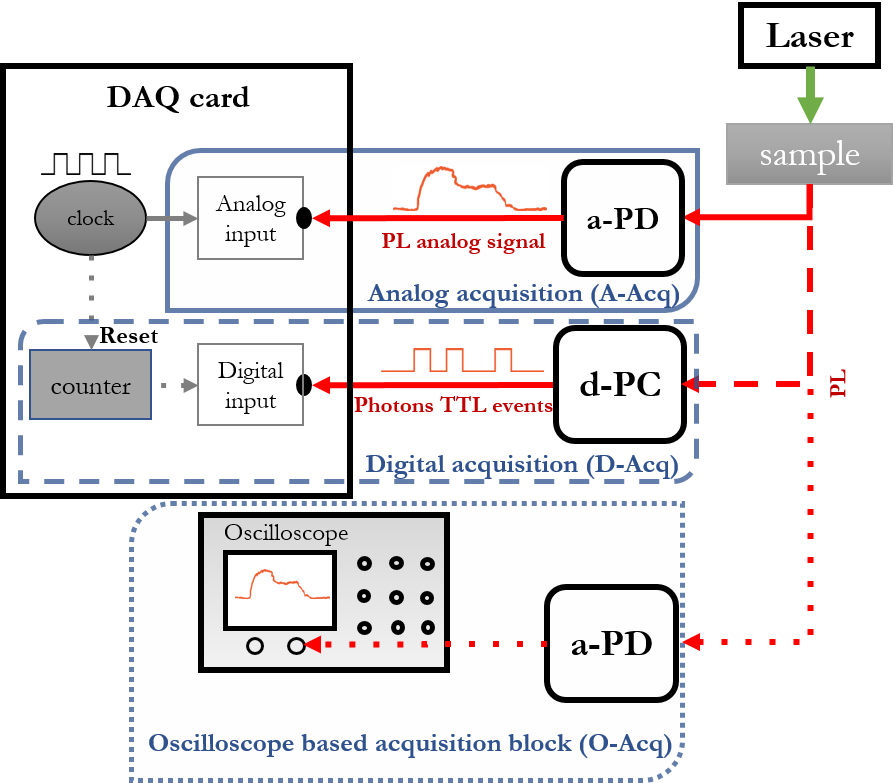
Figure 6: Hardware connections for monitoring a photoluminescence signal. The solid and dashed/dotted lines indicate the three hardware alternatives. The green color refers to the pumping beam and the red to the sample photoluminescence (PL). DAQ card internal connections are shown in gray. The analog, digital and oscilloscope-based acquisition blocks introduced here, are also used in Fig.s 7, 8, and 9 along with the same conventions.

III.2 Confocal scanning

In confocal microscopy, a scanning device (such as a piezo stage or a scanning mirror) is controlled while the sample PL is monitored. Synchronizing the two allows to attribute to each pixels its corresponding PL intensity, creating an image. As illustrated in Fig. 7, these controls and PL monitoring are commonly performed with a DAQ card in which an analog output is used for each spatial axes $(x),(y)$ and $(z)$. The measurement is performed by generating a sync signal of frequency $f_{sync}$ in the acquisition card and three step-ramp functions ranging from the lowest to the highest voltage are sent to the control ports of the scanning device. Each sync period therefore corresponds to a specific position of the scanning device for which the PL is collected. The sync frequency and order of the generated step ramp functions are eventually used to build the PL image.

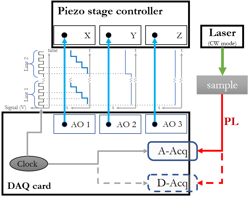
Figure 7: Hardware connections and synchronization links for confocal scanning. The analog and digital data acquisition blocks are introduced in Fig. 6.

III.3 CW ODMR

Continuous wave ODMR spectra are measured in a similar way, with the difference that the sweep is applied on the MW frequency instead of the beam (or sample) position. Each optical intensity must be attributed to the corresponding MW frequency. As described in Sec. I.4, the plot of the PL versus MW frequency mirrors the magnetic resonance spectrum. As reported in Fig. 8 the DAQ sends a TTL sync signal to the MW source and triggers frequency change while the corresponding PL signal is recorded simultaneously.

In case of using an oscilloscope for acquisition, the MW source, set in frequency modulation mode, becomes the synchronization master. It sends either a sweep or a TTL signal with the same period to a second input of the oscilloscope to trigger at the beginning of each sweep. The horizontal temporal scale of the oscilloscope can then be adjusted to display the PL as a function of the frequency. In the case of using a VCO, the frequency has to be set by an external voltage source, such as generated by a DAQ or waveform generator. The visualization on an oscilloscope can be performed in the same way.

Typical MW sources offer two modes to change the MW frequency: sweep and list. In the sweep mode, the minimum and maximum frequency and the step size are defined. As the MW generator receives a TTL signal, it changes the frequency by the defined step. In the list mode, the list of frequencies are previously stored in the generator, then as a TTL signal is received, the frequency is changed to the next one in the list. The list mode allows to perform random sweeping of the MW frequency mitigating problems such as hysteresis due to frequency-dependent MW heating through the antenna resonance. In practice, the acquisition speed of a CW-ODMR spectrum is limited by how fast the MW generation hardware can switch the output frequency. This values is for example around 1 ms minimum per step for R&S SMF100A.

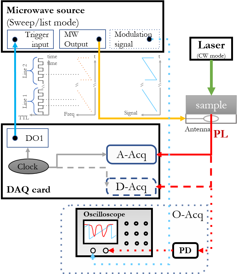
Figure 8: Hardware connections and synchronization links for CW-ODMR, MW connections are shown in orange. Other conventions are the same as in Fig. 6.

III.4 Pulsed measurements

As depicted in Fig. 9, pulsed measurements require synchronizing the laser and MW pulses with the optical signal acquisition. A pulse generator sends a TTL signal to command the laser and MW output switch. An additional TTL signal is also generated within the pulse generator to trigger the acquisition and set the time reference for each measurement. This signal is sent to the DAQ or oscilloscope. For each data point of a pulsed experiment, the optical signal is analyzed against the change of one variable (e.g., duration of the MW pulse or wait time between MW and laser pulses, see Sec.I.4).

Averaging strategies

— We discuss two different options, where $i\in\{1;P\}$ labels the value of a parameter (e.g. waiting time) to be swept among $P$ values and $N$ is the number of repetition over which the signal is to be averaged.

• A first averaging method is denoted as $"NP"$, where each $i^{th}$ pulse sequence is individually repeated $N$ times, before moving to the next parameter value from the $1^{st}$ to the $P^{th}$.

• In the second one, denoted as $"PN"$, a full series of $P$ sequences (consisting of $P+1$ optical pulses since the first only serves as initial polarization) is sent at once while the PL is recorded. This sequence is then repeated $N$ times to reach the desired signal to noise ratio. In this method, a slow varying noise similarly affects signals corresponding to all parameter values and is therefore averaged out. It also allows to monitor how the signal to noise ratio improves over the successive repetitions. However, it demands sufficient time resolution to isolate signals from each pulse sequence making it hardly compatible with the use of a camera. It also requires digitizing and storing the full sequence at once, which also limits the use of an oscilloscope (see Sec. II.1.4).

Synchronization strategies

— In either cases, two distinct synchronization methods are possible:

• ‘Sync method 1’: Only two TTL sync pulses are generated, at the start and at end of each series of $N$ (or $P$) sequences.The incoming optical signal is continuously recorded between the initial and final pulses according to the sampling rate. The position of each pulse is then calculated by software (see Sec. V.3). This cannot be done when using an oscilloscope.

• ‘Sync method 2’: A TTL pulse is sent at the beginning of each pulse to be either timestamped by the counter with a DAQ card or used to trigger the oscilloscope.

Fig. 9b depicts two out of the four possible combinations of averaging and synchronization strategies in the case of a Rabi oscillation measurements.

Implementation with a DAQ card

— The implementation of aforementioned methods with an NI card can be elaborated based on the type of the acquired signal.

• In the analog case, the a-PD signal is sent to an analog input channel of the DAQ card. As discussed in section III.1, the ADC captures and saves the analog signal into the buffer until it is read out. With ‘Sync method 1’, the generated sync pulses are transmitted to another analog channel of the DAQ card and the acquisition starts as soon as it receives a sync pulse. As a consequence, the optical signal is recorded even when the laser is off. Identification of each pulse then requires post-processing as described in Sec. V. With ´Sync method 2’, the generated sync pulses are sent to a digital channel of the DAQ card. The channel is adjusted to acquire the pulses during the laser pulse windows using start edge trigger and pause trigger protocols of the DAQ card.

• Acquiring data from a d-PC, however, demands time-tagging as described in section III.1. Similarly, the ‘sync method 1’ records all the photon received. the pulses are found and reconstructed by post-processing. With ‘sync method 2’ the trigger signals are time-tagged and mark the beginning of each pulse.

One chooses the synchronization method depending on hardware limitations and desired averaging strategy discussed above.

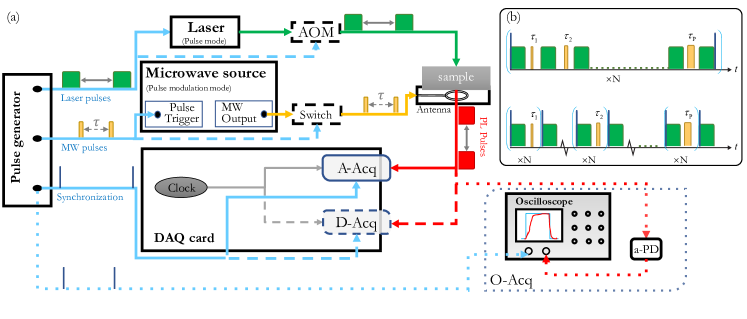
Figure 9: (a) Hardware connections and synchronization links for pulsed experiments. Solid and dashed lines indicate different alternatives depending on available hardware. (For example, if the laser permits pulsed modulation, the AOM is not required.) (b) Averaging and synchronization strategies in the case of a Rabi measurement. Top: $PN$ strategy with ‘Sync method 1’, Bottom: $NP$ method with ‘Sync method 2’

IV Qudi, an open-source interface for ODMR experiments

As discussed in Secs. II and III, the use of a dedicated software can be necessary to control a confocal microscope or deal with photon counting. It can also automatize the control of ODMR instruments to speedup the measurements and ease their reproducibility, either for fundamental studies or application developments. Ideally, the software interface should deal with both single photon counters in low light conditions and analog photodetectors, process confocal and wide-field images, and freely combine different measurement parameters and methods.

Several options exist for coding such interface program. On the one hand, mid-level languages such as C++ or FORTRAN, down to the lower-level ones such as assembly, offer the best possibilities to optimize computer resources. They are often the best option for demanding computational physics and simulations, artificial intelligence related research, or for processing of complex or voluminous data Mirams et al. (2013). On the other hand, higher level programming languages, such as Python or Java, greatly facilitate design, development and maintenance of codes. They also ensure better portability between different hardware configurations. They are therefore particularly appropriate for interfacing laboratory experiments Cao et al. (2013); Chapman and Chang (2000). A comparison between programming languages including C, C++, Java and Python can be found in Prechelt (2000).

Among others, Labview (for Laboratory Virtual Instrument Engineering Workbench), a proprietary programming environment developed by National Instruments Bitter, Mohiuddin, and Nawrocki (2006), offers a graphical diagram coding style making it more intuitive to newcomers in programming. Moreover, it permits to easily interface with laboratory instruments and offers libraries for signal generation, data acquisition and processing that allow to rapidly setup basic experiments. However, when the experimental complexity increases, this graphical programming style can become difficult to handle. It also remains incompatible with versioning and collaborative tools such as Github for sharing codes and subroutine within a community.

In this context, Python, a high-level programming language, offers a great alternative Cahn and Russo (2007). Coding environments and interpreters being open source, it is particularly popular and used in various domains, including experiment control. It supports versatile and efficient community-developed libraries. Moreover, it offers sufficient level of abstraction to allow portability between computers of different configurations and making it upgradeable to new functionalities, embeds efficient multi-threading and signaling capabilities allowing for parallel operations (data acquisition, processing and display).

Here, we introduce Qudi, an open-source Python code dedicated to ODMR measurements. First presented in Binder et al. (2017), it is an open-source collaborative project shared on Github and it benefits from a well programmed Python-based architecture. We first present Qudi’s original features and the ones we added to improve its performance and extend its applicability. We then detail Qudi’s architecture and presents how to configure and use it.The official Qudi’s version is available on GithubQud (a) and a general documentation based on developers "in code" comments along with a brief general tutorial can be found here Qud (b). For those not already merged within the official Github, the added features can be found on our Github page forked from it Our (a).

IV.1 Qudi’s features

Qudi Binder et al. (2017); Qud (a); Our (a), initially released in 2017, integrates modules for performing ODMR experiments, instrument control, and real-time data acquisition and processing. It enables fast imaging by scanning the beam position while collecting luminescence. Qudi can locate ODMR emitters and track them during acquisition, compensating for sample drift. It is particularly useful for studying nanoparticles in liquid suspensions McGuinness et al. (2011); Sigaeva et al. (2022b). It provides useful tools for interfacing a scanning confocal microscope by controlling piezo-based nanopositioning stages or scanning mirrors and collecting the optical emission signal. Possibilities include in-plane scanning $(xy)$, $z$-stack acquisitions (to obtain 3D images), out of plane cross-sections $(xz)$ or $(yz)$ as well as any other direction cuts depending on the wiring and instrument. Associated to confocal microscope hardware (see Sec. II.1), Qudi can locate and track ODMR emitters, compensating for sample drift. This feature is particularly interesting when dealing with nanoparticles in a liquid suspension such as in biomedical applications McGuinness et al. (2011); Sigaeva et al. (2022b).

Qudi efficiently controls the instruments required for acquiring CW ODMR spectra and determining spin resonance frequencies. Real-time fitting of analytical curves on ODMR data allows for adjustment of acquisition parameters and quick sharing of results with collaborators. In addition to the CW ODMR signal, Qudi is designed for the study of spin dynamics with pulse sequences such as for measuring longitudinal spin relaxation curves ($T_{1}$), Rabi oscilations, Ramsey ($T^{*}_{2}$) or Hahn Echo ($T_{2}$) sequences (see Sec. I.4). It can control the pulse generator for triggering laser and MW pulses (see Sec. II.3) in a synchronous manner with the collection of the photoluminescence (see Sec. III.4). It also enables the design of complex pulse sequences, including dynamical decoupling sequences. Predefined methods like XY8 pulses are available via the graphical interface, and new pulse sequences can be easily added to the program Qud (c).

Qudi offers tools for on-the-go pulse extraction, analysis, and automated experimental parameter settings. This simplifies long measurement sequences across different materials. Using Qudi’s Jupiter notebooks Qud (d), one can design and automate independent experiments to vary multiple control variables, enabling efficient exploration of parameter space.

Module	Original features	Added features
	Analog acquisition	Acquisition with oscilloscope
Counting	Digital acquisition	Faster analog and digital DAQ acquisition
	Analog acquisition	Acquisition with oscilloscope
Confocal	Digital acquisition	Control with Pulse Streamer
		Arbitrary/random MW sweep
		Acquisition with oscilloscope
		Acquisition with Spectrometer
ODMR	Analog acquisition Digital acquisition	Lock-in detection*
		Analog acquisition with DAQ
		Analog acquisition with oscilloscope
		Digital acquisition with DAQ
		Pulse extraction improved
Pulsed	Digital acquisition with time tagging device	New pulse sequences

Table 3: Summary of Qudi main features in the original release Qud (a) and in our upgraded version Our (a). *Under development.

The initial version of Qudi was focused for experiments on single quantum emitters, thus requiring digital single photon counting modules as well as time tagging electronics in the pulsed measurements. In order to broaden its contextual applicability, we added several features.

At first, a direct oscilloscope interface was implemented for data acquisition (see Sec. II.1.4) while, conversly, NI card (or similar DAQ device)’s digital inputs can now also be used as a fast event counter and the minimum temporal resolution has been reduced to half the card internal clock period, making it sufficient for ODMR experiments without need of dedicated time tagging instruments.

Two strategies for photon counting were implemented (see Sec. III.1) and a new logic for pulsed measurements was coded to enhance acquisition speed and eliminate the need for post-treatment and pulse extraction described in Sec. III.4. Pulsed measurements using analog signals were also added, making the system compatible with analog photodiode signals for studies of ensemble (see Sec. II.1.1). Analog acquisition in CW-ODMR was also improved by increasing the sample rate per frequency sweep, optimizing signal-to-noise ratio (see Sec. III.1).

Finally, an arbitrary/random MW frequency sweep was added to minimize thermal effects of the resonator on the ODMR signal and an optical spectrometer module was incorporated for ODMR signal acquisition using a user-specified spectral window. The summary of the added features to the Qudi platform is shown in Table 3.

IV.2 Main architecture

Qudi is made of different modules that are loaded and connected together by a manager component. The science modules responsible for experiment control are divided into three categories: GUI (graphical user interface), logic, and hardware. As detailed in the following, this division is based on a clear separation of tasks among the categories and offers a reliable and flexible software architecture and simultaneous (multi-threading) acquisition, data treatment and visualization. Importantly, the setting of those modules and the links between them is to be defined in a configuration file (See Sec. IV.3).The important notion of hardware interface (higher abstraction level of hardware module) is also introduced.

IV.2.1 Modules

GUI modules —

They create an interactive graphical interface that allows the user to control the experiment and to visualize the acquired data. In particular, the GUI allows to start and stop the acquisition, to adjust the experimental parameters (e.g. MW power, frequency sweep range, acquisition time…), to save the data and to fit them with pre-defined functions, simply pushing buttons or inserting values into the interactive windows. Changes made in the graphic interface, such as a pushed button or a modified parameter, trigger a broadcast signal sent to the related logic modules. Although GUI modules offer an intuitive and efficient way to interact with the logic modules, Qudi can also be fully functional without them via the integrated Ipython console or via a Jupyter notebook.

Logic modules —

They form the basis of every experiment designed in Qudi. Their main function is to coordinate the different tasks necessary to perform a complete experiment. They serve as a bridge between the two other kinds of modules. On one side they receive the emitted signals from the GUI modules and they send others to the hardware modules to configure the instruments sig . Conversely, they gather and analyze data coming from the hardware modules and pass them to the GUI modules for display.

Each experiment depends on a variety of generic tasks that are common to different types of measurements, such as fitting appropriate curves, saving data, etc. Therefore, rather than having a single logic module for each experiment performing all these tasks, they are divided in multiple logic modules used in a versatile manner. Besides communication with hardware and GUI modules, each logic module can receive inputs from and send outputs to other related logic modules. Note that logic modules are the only ones allowed to talk to modules of the same category.

Hardware modules —

The main task of these modules is to allow an effective communication between the logic modules and the specific hardware. Receiving orders from the logic modules, they run the equipment drivers (often provided by the supplier) to act onto the experiment. They also send the output signals of the instruments to the logic modules, to be further analyzed, displayed and eventually saved. Moreover, hardware modules can also work as virtual dummy or mock hardware, emulating the functionality of a real device. This possibility can be very helpful for configuring a new setup. As an example, modules and links between them that are required for the four typical experiments described in Sec. III are presented in Figure 10.

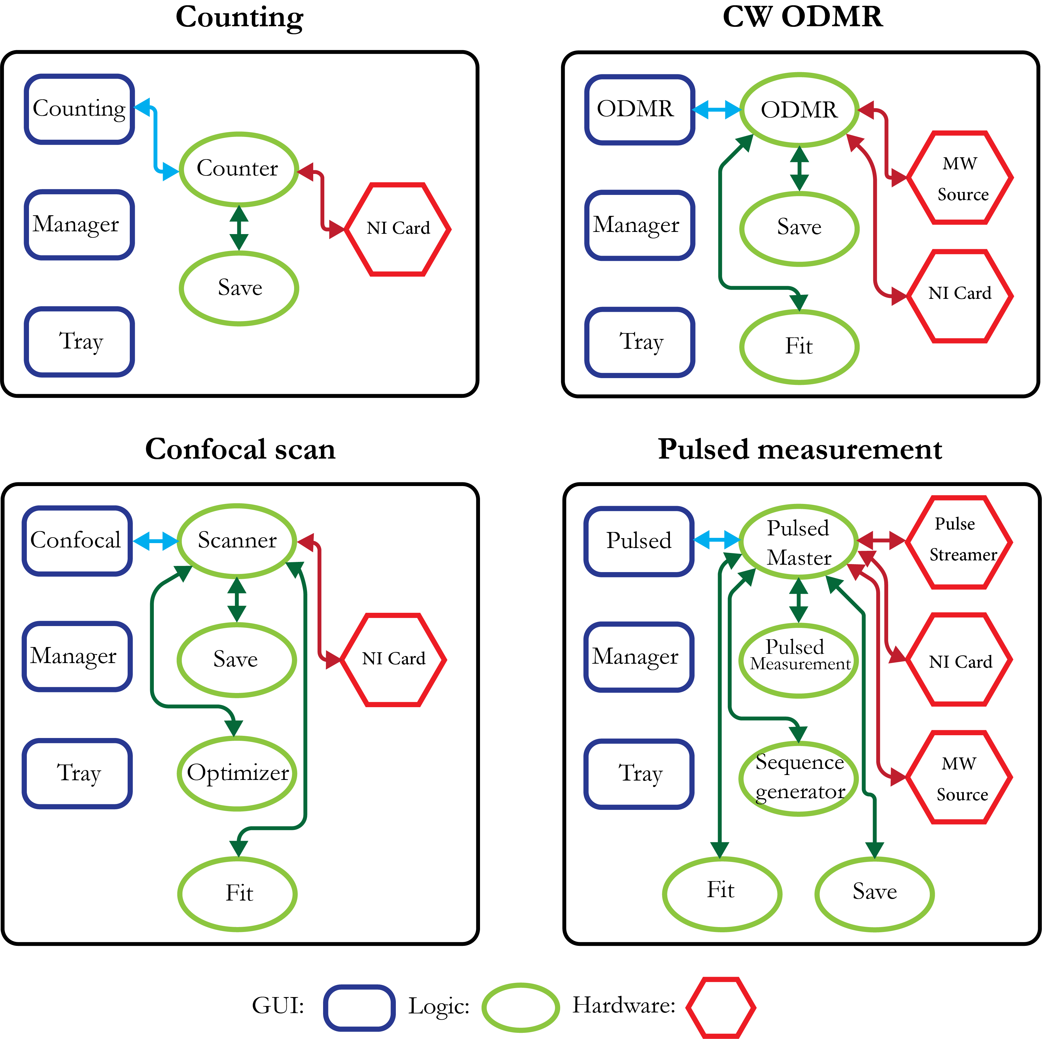
Figure 10: Block diagrams for the software connections of counting, confocal scan, CW ODMR, and pulsed measurement which needs to be included in the configuration file.

IV.2.2 Hardware interfaces

Even if a set of instruments have common features for performing similar tasks, there is, between different models and suppliers, a wide difference in command structure, grammar and connection methods. In order to handle this complexity, a specific interface is defined for each category of instruments. In the context of object oriented programming, hardware modules are classes that inherit from hardware interfaces. The running of a laboratory equipment consists in defining and operating instances (objects) from the instruments-related classes. The interface therefore consists of a set of functions that each hardware module within the same category must implement. Therefore, each instrument used in an experiment should have its own class compatible with the related interface class in Qudi. This class needs to control the instrument while respecting constraints on its operation as specified in its data sheet. To accomplish this task, the class may use drivers provided by the instrument’s manufacturer. Various instruments have already been introduced in Qudi in different categories (such as spectrometers, cameras, MW generators, pulse generators, etc.). However, due to the wide variety of systems, applications, suppliers and models available, it may be necessary to add a new device or modify the class for an instrument whose model is slightly different from the one defined in the code.

IV.3 Utilization

Installing Qudi is rather straightforward from Qudi Documentation's instructions doc . It can be cloned from the original Qud (a) or our Our (a) Github.

Performing experiments with Qudi, also requires to tune it specifically for the user’s hardware environment and specific needs by writing a configuration file, which, in particular, defines the connections between the modules that are used such as represented in Figure 10. Besides, installing an instrument that is not yet supported requires to write the corresponding hardware module class (see above section IV.2.1). Finally, for important coding project such as Qudi, it can be useful to configure the Python environment to ensure the good functioning of the different packages and libraries that are used in different places of the code. This can be performed through a conda environment installer such as the one called Anaconda available in the Github subfolder qudi\tools.

The utilization of the module we added in our Github Our (a) (see Sec. IV.1) is detailed in Babashah (2023), Our (b).

In the following section, we will focus on the characterization of an NV center ensemble to propose some practical advice and discuss good practices when performing typical ODMR experiments with a home-build confocal microscope (see part. II) controlled using Qudi.

V Good practices for ODMR measurements: NV Center characterization

As described in Sec. I.4 the main figures of merit characterizing an ODMR system are the longitudinal spin relaxation time $T_{1}$, dephasing time $T_{2}^{*}$ and coherence time $T_{2}$ (the latter being dependent on the type of echo sequence used to measure it). In this section, we describe the procedure and methods to reliably perform these measurements such as presented in Fig. 3. As an illustration, we characterize a small ensemble of NV centers in bulk diamond using a single pixel detector in a confocal geometry (see Sec. II.1.1). While an extensive review on optimizing sensitivity with NV centers can be found in Barry et al. (2020), we aim here to provide practical advice on how to easily reach good measurement quality in terms of acquisition speed, contrast and repeatability.

The measurements presented in this section are performed on a bulk diamond sample enriched in NV centers and provided by Appsilon B.V. Other possibilities for commercial diamond providers are summarized in Table 2. It should be noted that the figures of merit discussed here can vary significantly depending on the material quality. For practical purposes, we provide throughout the section typical values for these figures of merit in an NV ensemble. They are given for a sample at room temperature, in the absence of external perturbation (magnetic field, electric field, pressure, etc.).

V.1 Procedure

The sample is first placed in the optical setup and its position adjusted to match the object focal plane of the objective. A confocal scan allows to image the sample and identify the region of interest. At this step, further alignment of the setup to ensure that maximum signal is emitted by and collected from the NV centers is possible. A single NV center can provide photon count rates above $100\text{\,}\mathrm{kHz}$ when using a numerical aperture exceeding 0.9 and a laser excitation power in the mW range. The total PL depends linearly on the number of NVs in the ensemble. According to the level of brightness of the sample and collection efficiency of the setup, a proper detector (e.g. photon counter or analog photodiode) and possibly a neutral density filter are selected. Then, we use Qudi ODMR interface to perform a CW-ODMR scan. The goal of this step is to adjust the bias magnetic field (by monitoring the different resonances in the spectrum) and to identify the resonance frequency that will be used for the following pulsed measurements.

One specificity with NVs is that each center can take one of the four $(111)$ crystallographic orientations of the diamond lattice. Considering the two allowed MW transitions from $\left|m_{s}=0\right>$ to $\left|m_{s}=-1\right>$ and $\left|m_{s}=+1\right>$, this can lead to eight distinct resonances (that are further split by hyperfine interaction) whose frequencies correspond to the projection of the magnetic field along each orientation. It allows to perform vectorial magnetometry Maertz et al. (2010); Chipaux et al. (2015b), even without biased applied fieldsLenz et al. (2021); Wang et al. (2022). Certain applications require a specific magnetic field alignment (see Sec. II.4). In this example, we target a bias field such that the Zeeman splitting for at least one NV orientation is different from all other orientations, i.e at least one pair of transitions in the spectrum is non-degenerate.

We select a MW frequency resonant with one of these two transitions (corresponding to either $\left|m_{s}=-1\right>$ or $\left|m_{s}=+1\right>$) and perform pulsed measurements to characterize $T_{1}$, $T_{2}$ and $T_{2}^{*}$. To this end, we move to Qudi interface for pulsed Measurement. Rabi oscillations are first measured to determine the duration of a $\pi$-pulse which is half the oscillation period. We note in passing that the decay of Rabi oscillations is not simply related to any of the time constants mentioned above because increasing the MW pulse duration reduces is spectral bandwidth and thus progressively filters a smaller set of NV centers among the inhomogeneously broadened ensemble. Since a good estimate of $T_{2}^{*}$ can be obtained from the CW-ODMR linewidth (in the limit of low MW powers) it is recommended to use sufficient MW power in the pulse sequences so that the $\pi$-pulse is shorter than $T_{2}^{*}$ in order to efficiently drive all NV centers in the ensemble. The last step consists in applying each of the dedicated pulse sequences to extract $T_{1}$, $T_{2}$ and $T_{2}^{*}$, previously presented in Sec. I.4.

V.2 CW ODMR

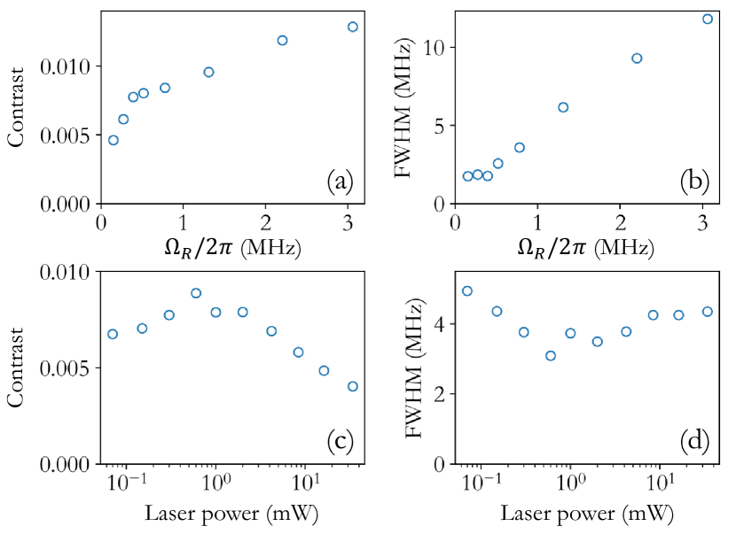
Figure 11: (a, c) Contrast and (b, d) FWHM of a single resonance in the CW ODMR spectrum, versus (a, b) MW Rabi frequency and (c, d) laser power.

In order to perform CW ODMR with highest possible contrast and narrow linewidth, a compromise must be reached in terms of both MW and laser powers, as illustrated in Fig. 11. While the optical excitation rate must be faster than the $1/T_{1}$ relaxation rate to ensure that all spins are well polarized, a too high rate can decrease the ODMR contrast by competing with the MW excitation and preventing a large population difference between states $\left|m_{s}=0\right>$ and $\left|m_{s}=1\right>$ Jensen et al. (2013). On the other hand, while increasing the MW power first enhances the contrast, it then broadens the resonances through power broadeningDréau et al. (2011) and eventually reaches saturation of the spin transition.

As practical guidelines (for NV ensembles) the optimal laser power is the one maximizing contrast and the optimal MW power is the highest power for which the linewidth remain close to the $T_{2}^{*}$ limit. For further optimization, the optimum condition for the laser and MW power can be derived analytically using a rate equation approach Dréau et al. (2011); Jensen et al. (2013). Typically, a single NV center exhibit an ODMR contrast above $10\%$. For an ensemble with 4 possible NV orientations, this results in best contrast of around $2\%$ for each resonance in the ODMR spectrum, close to the values reported in Fig. 11. The presence of other photoluminsecent defects, such as neutral NV0, causes a reduction of the ODMR contrast.

V.3 Pulsed experiments

To improve the quality of a pulsed experiment several factors should be taken into account. Some are general to all pulsed protocols, while others are more specific. Common requirements for all pulsed experiments are reliable initialization and readout. Laser pulse duration needs to be long enough to ensure maximum polarization in state $\left|m_{s}=0\right>$. The characteristic time for spin polarization depends on the optical power density and typically ranges from $100\text{\,}\mathrm{ns}$ to $1\text{\,}\mathrm{\SIUnitSymbolMicro s}$. For NV centers, the initialization pulse must be followed by a waiting time, typically $1~{}{\mathrm{\mu s}}$, to allow relaxation of population trapped in the singlet state towards the ground state $\left|m_{s}=0\right>$ Robledo et al. (2011). The characteristic polarization time also impacts the readout phase. Depending on the time resolution of the hardware (see Sec. II.1.4 and III.1), it can be convenient to reduce the laser power, to polarize the spin slower and be able to resolve it dynamics as in Fig. 12. The duration of the optical pulse needs to be adjusted accordingly.

In the case of ‘Synchronization method 1’ (see Sec. III.4) in which only the beginning and the end of a sequence is triggered, it is necessary to locate each pulse within the entire recorded optical signal. In this case, two standard approaches are implemented in Qudi for pulse recognition. The first uses a threshold value to identify rising and falling edges of a pulse. The second relies on a convolution of the signal with a Gaussian distribution and takes its first derivative, resulting in a pulse identification signal $S_{p}(t)$ given by:

$${S_{p}}(t)=\frac{{d}}{{dt}}\left[{S_{r}}(t)\otimes\frac{1}{{\sigma\sqrt{2\pi}}}{e^{-\frac{1}{2}{{(\frac{{t}}{\sigma})}^{2}}}}\right]$$ (8)

where $t$ represents the time and $S_{r}(t)$ is the raw signal acquired during the pulsed measurement; $\sigma$ is the standard deviation for the Gaussian filter. Rising and falling edges of pulses correspond to local maxima and minima of ${S_{p}}(t)$. The Gaussian filter allows to smooth the signal and reduces false pulse detection. This second method is thus generally more robust than the first one. Optimal extraction is achieved by adjusting the parameter $\sigma$.

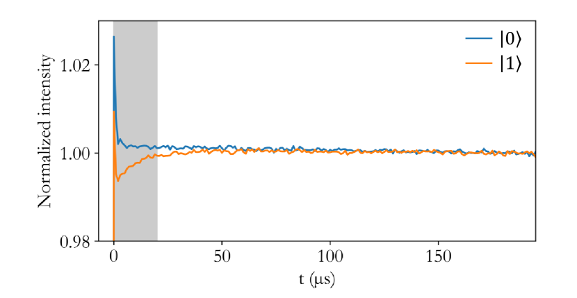
Figure 12: Normalized luminescence intensity during the readout laser pulse, for spins initialized in state $\left|0\right>$ (blue curve) and $\left|1\right>$ (orange, using a $\pi$-pulse between optical pumping and readout), collected with NA 0.65 objective and 35 mW incident laser power. The shaded gray region indicates a good choice of time window for signal integration, yielding high SNR.

Figure 12 displays the time evolution of luminescence intensity during a laser pulse starting at $t=0$, for spins initially prepared either in $\left|m_{s}=0\right>$ or $\left|m_{s}=1\right>$. The different levels of PL in the two cases and the spin polarization dynamics, are clearly resolved. To obtain a measure of the spin projection along the quantization axis the PL intensity is integrated over an early time window marked as gray shaded area, and normalized to the PL intensity integrated at the end of the pulse (not represented), when spins are polarized again. It allows to compensate possible slow fluctuations of the laser intensity or collection efficiency.

To maximize the signal to noise ratio, the time window should start with the laser pulse, where the PL difference between $\left|m_{s}=0\right>$ and $\left|m_{s}=1\right>$ is maximal. If the initial time of a pulse is not properly identified by the pulse extraction method for all pulses in the sequence (e.g. due to slow laser rise time), the resulting timing jitter translates into noise on the total integrated signal. In this case excluding very early times of the readout pulse can be beneficial.

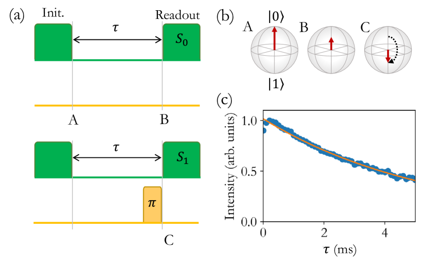
Figure 13: (a) Pulse protocol for optimized $T_{1}$ measurement, with the addition of a $\pi$-pulse to extract $S_{1}$. (b) Bloch sphere representation of the spin state at times of the pulse protocol indicated in (a). (c) Resulting signal versus delay $\tau$, fitted with an exponential decay (solid line)

Several other sources of noise can affect readout fidelity. Among them, some are spin-independent, for example due to NV ionization and NV- recombination caused by the laser pulse Aslam et al. (2013); Giri et al. (2018). A powerful solution to suppress this kind of noise is to repeat the pulsed protocol but inverse the spin state onto $\left|m_{s}=1\right>$ just before readout using a $\pi$-pulse as illustrated in Fig. 13  Jarmola et al. (2012). The extracted signals with and without inserted $\pi$-pulse are labeled $S_{1}$ and $S_{0}$, respectively. The expectation value of the spin state projection is linearly related to the difference signal $S_{0}-S_{1}$ from which spin-independent common noise is removed. The result of this procedure for a $T_{1}$ measurement is illustrated in Fig. 13.

Another important source of artifacts arises when the dark time $\Delta T$ between consecutive laser pulses is swept. As mentioned in Sec. II.3 it can lead to variation in laser pulse intensities over for the entire sequence. In most cases, a simple solution is to keep $\Delta T$ constant, adjusting some waiting times before and after the microwave pulses accordingly, as long as $\Delta T\ll T_{1}$. It is however not possible for a $T_{1}$ measurement. Fortunately, the protocol discussed just above allows to partially mitigate such artifact by normalizing the signal by $S_{0}+S_{1}$. Such protocol also allows to extract a relevant signal even when the setup temporal resolution does not allow to resolve the pulse dynamic, e.g. when using a camera in a widefield configuration.

A final knob for optimization of pulsed measurements is in the definition of $\pi$, $\pi/2$ and other pulses. The duration of such pulses is in principle extracted from the measured period of Rabi oscillations. However, in practice small deviations can arise, e.g. due to not perfectly square MW pulses and fitting errors. It is thus good practice to perform a calibration step. To this end, we use a Hahn echo sequence with fixed delay and monitor the echo amplitude for varying initial, central and final MW pulses. The result of this procedure is illustrated in Fig. 14, where the initial and final pulses are half the central pulse. Every second sequence, we also replace the final pulse with a $3\pi/2$-pulse, to apply the above common noise rejection strategy. The optimum pulse duration corresponds to the simultaneous maximum echo amplitude when the final pulse is $\pi/2$ and minimum when it is $3\pi/2$. This ensures maximum contrast for a $T_{2}$ measurement, using the Hahn echo sequence (Fig. 3(d)). The calibrated $\pi/2$-pulse is also used for $T_{2}^{*}$ measurement using Ramsey interferometry (Fig. 3(c)).

As stated earlier, $T_{1}$, $T_{2}$ and $T_{2}^{*}$ depend greatly on the diamond quality, as well as on the presence of external perturbations. For an NV ensemble with moderate concentration (below 1ppm), $T_{1}$ is usually on the order of several milliseconds, $T_{2}^{*}\approx 0.5-1\mathrm{\mu s}$ and $T_{2}$ is limited to few 10s of $\mathrm{\mu s}$ with a simple spin-echo sequence, but can be extended to several 100 $\mathrm{\mu s}$ with better dynamical decoupling protocols. The interested reader should refer to e.g. Ref. Barry et al. (2020) for a more quantitative, in-depth discussion of these coherence times, which is beyond the scope of the present paper.

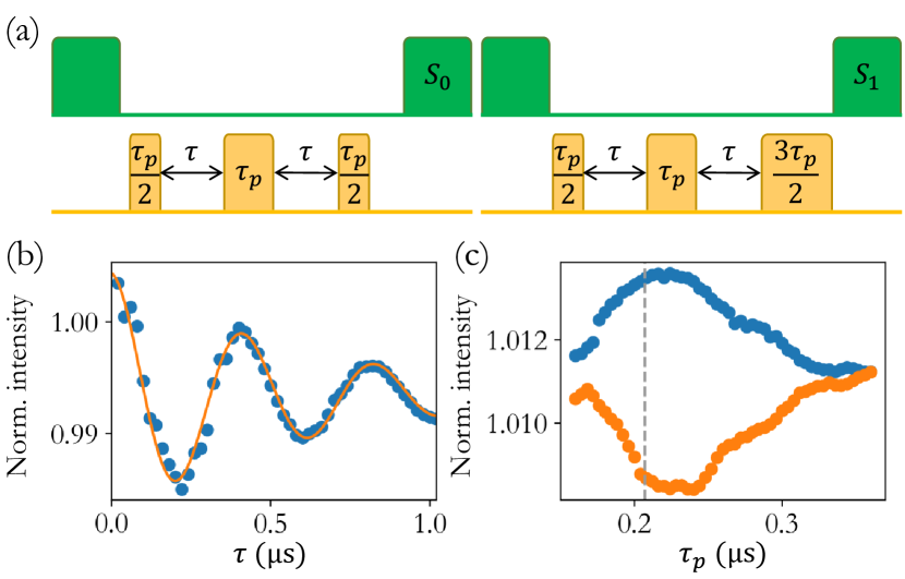
Figure 14: (a) Hahn echo sequence used for optimization of $\pi$ and $\pi/2$-pulses. (b) Rabi oscillations with cosine fit (solid line). (c) Echo amplitude versus pulse duration $\tau_{p}$. The delay is $\tau=500~{}\mathrm{ns}$. Dashed line indicates the $\pi$-pulse duration extracted from fit of Rabi oscillations in (b) which appears not to be optimal.

Conclusions and perspectives

In this article, we present the settings of an experimental breadboard for ODMR experiments with both commercially available instruments and an open-source interface. In particular, we show that a relatively inexpensive acquisition card equipped with analog-to-digital converter, together with our upgrades on the Python-based software Qudi, allow anyone with minimal experimental skills to setup ODMR instrumentation capable of advanced magnetic resonance pulse sequences and address both individual optically-active spin-systems and large ensembles. We believe that our work will help foster the development of ODMR studies and their applications to sensing and metrology, quantum technologies, and material science, while also making ODRM methods more accessible to non-specialists. We encourage Qudi users to develop new instrument modules and make them available on GitHub to participate to wider openness and collaboration in research. We conclude by mentioning a few envisioned directions for both hardware and software developments in the coming years.

Performing ODMR at room temperature without space constraints does not present significant hardware challenges anymore. Yet, implementing similar measurements in confined environments, in ultra-high vacuum or at cryogenic temperatures, can rapidly become much more complex. While optical excitation and collection through free space or optical fiber is usually feasible in such circumstances, it can be challenging to locally provide enough MW power (without spurious heating) and apply strong enough and precisely oriented bias magnetic fields. Therefore, an integrated solution in the form of a chip-scale cryo-compatible device, with footprint below a few square millimeters, and which embeds a d.c. supplied MW oscillator and antenna, would be a valuable commodity for ODMR experiments. Such devices have already been developed in the context of conventional electron and nuclear spin resonance spectroscopy Matheoud, Sahin, and Boero (2018).

Regarding MW generation, voltage-controlled oscillators (VCOs) are inexpensive and compact alternatives to high-end MW sources, and lowering their phase noise would make them more useful for advanced measurements. Design of MW antennas delivering strong and homogeneous driving fields over wide areas is still in progress.

For single-emitter ODMR, both the digital single photon counting modules and the time tagging electronics drive the costs of the setup higher (typically 5’000 EUR each). As a cheaper alternative to the latter, FPGAs can be programmed for photon counting to yield much better temporal resolution than an NI card. An open-source package based on a commonly available FPGA for a do-it-yourself time tagger would make single emitter measurements more accessible.

For generating complex, long and low noise pulse sequences, NI cards reach their limits. As above, FPGA-based open-source solutions have the potential to make such experiments accessible at lower costs and with a high degree of customization for specific needs.

Author declarations

Conflict of Interest

The authors declare no conflicts of interest.

Author Contributions

H.S and H.B. contributed equally to this work. H.B contributed significantly to the coding and assisted with the writing. H.S played a key role in writing the paper and valuably contributed to the coding. E.L contributed to the writing and revisions. H.B built the characterization setup for measurements. V.G. conducted, analyzed, and reported the measurements. M.C guided the writing throughout the project. M.C and C.G supervised the work and contributed to the writing and revisions.

Data availability

The original and updated version of qudi are available on github Qud (a); Our (a).

Bibliography

Bibliography

- Ohanian (1998) H. C. Ohanian, “What is spin?” American Journal of Physics 54, 500 (1998).
- Dowling and Milburn (2003) J. P. Dowling and G. J. Milburn, “Quantum technology: the second quantum revolution,” Philosophical Transactions of the Royal Society of London. Series A: Mathematical, Physical and Engineering Sciences 361, 1655–1674 (2003).
- Vandersypen et al. (2017) L. M. K. Vandersypen, H. Bluhm, J. S. Clarke, A. S. Dzurak, R. Ishihara, A. Morello, D. J. Reilly, L. R. Schreiber, and M. Veldhorst, “Interfacing spin qubits in quantum dots and donors-hot, dense, and coherent,” npj Quantum Information 3, 1–10 (2017).
- Zhang et al. (2018a) X. Zhang, , H.-O. Li, , K. Wang, , G. Cao, , M. Xiao, , and G.-P. Guo, “Qubits based on semiconductor quantum dots*,” Chinese Physics B 27, 020305 (2018a).
- Chang, Hsiao, and Su (2018) H.-C. Chang, W. W.-W. Hsiao, and M.-C. Su, “Color Centers in Diamond,” Fluorescent Nanodiamonds , 37–54 (2018).
- Castelletto and Boretti (2020) S. Castelletto and A. Boretti, “Silicon carbide color centers for quantum applications,” Journal of Physics: Photonics 2, 022001 (2020).
- Bertaina et al. (2007) S. Bertaina, S. Gambarelli, A. Tkachuk, I. N. Kurkin, B. Malkin, A. Stepanov, and B. Barbara, “Rare-earth solid-state qubits,” Nature Nanotechnology 2, 39–42 (2007).
- Camenzind et al. (2018) L. C. Camenzind, L. Yu, P. Stano, J. D. Zimmerman, A. C. Gossard, D. Loss, and D. M. Zumbühl, “Hyperfine-phonon spin relaxation in a single-electron GaAs quantum dot,” Nature Communications 9, 1–6 (2018).
- Degen, Reinhard, and Cappellaro (2017) C. L. Degen, F. Reinhard, and P. Cappellaro, “Quantum sensing,” Reviews of modern physics 89, 035002 (2017).
- Wesenberg et al. (2009) J. H. Wesenberg, A. Ardavan, G. A. D. Briggs, J. J. Morton, R. J. Schoelkopf, D. I. Schuster, and K. Mølmer, “Quantum computing with an electron spin ensemble,” Physical Review Letters 103, 070502 (2009).
- Pezzagna and Meijer (2021) S. Pezzagna and J. Meijer, “Quantum computer based on color centers in diamond,” Applied Physics Reviews 8, 011308 (2021).
- Lescanne et al. (2020) R. Lescanne, S. Deléglise, E. Albertinale, U. Réglade, T. Capelle, E. Ivanov, T. Jacqmin, Z. Leghtas, and E. Flurin, “Irreversible Qubit-Photon Coupling for the Detection of Itinerant Microwave Photons,” Physical Review X 10, 021038 (2020).
- Dolde et al. (2014) F. Dolde, V. Bergholm, Y. Wang, I. Jakobi, B. Naydenov, S. Pezzagna, J. Meijer, F. Jelezko, P. Neumann, T. Schulte-Herbrüggen, J. Biamonte, and J. Wrachtrup, “High-fidelity spin entanglement using optimal control,” Nature Communications 5, 1–9 (2014).
- Blank et al. (2009) A. Blank, E. Suhovoy, R. Halevy, L. Shtirberg, and W. Harneit, “ESR imaging in solid phase down to sub-micron resolution: methodology and applications,” Physical Chemistry Chemical Physics 11, 6689–6699 (2009).
- Suter (2020) D. Suter, “Optical detection of magnetic resonance,” Magnetic Resonance 1, 115–139 (2020).
- Gugler et al. (2018) J. Gugler, T. Astner, A. Angerer, J. Schmiedmayer, J. Majer, and P. Mohn, “Ab initio calculation of the spin lattice relaxation time $T_1$ for nitrogen-vacancy centers in diamond,” PHYSICAL REVIEW B 98, 214442 (2018).
- Balasubramanian et al. (2009) G. Balasubramanian, P. Neumann, D. Twitchen, M. Markham, R. Kolesov, N. Mizuochi, J. Isoya, J. Achard, J. Beck, J. Tissler, V. Jacques, P. R. Hemmer, F. Jelezko, and J. Wrachtrup, “Ultralong spin coherence time in isotopically engineered diamond.” Nature materials 8, 383–387 (2009).
- Nishimura et al. (2020) K. Nishimura, H. Kouno, Y. Kawashima, K. Orihashi, S. Fujiwara, K. Tateishi, T. Uesaka, N. Kimizuka, and N. Yanai, “Materials chemistry of triplet dynamic nuclear polarization,” Chem. Commun. 56, 7217–7232 (2020).
- Binder et al. (2017) J. M. Binder, A. Stark, N. Tomek, J. Scheuer, F. Frank, K. D. Jahnke, C. Müller, S. Schmitt, M. H. Metsch, T. Unden, T. Gehring, A. Huck, U. L. Andersen, L. J. Rogers, and F. Jelezko, “Qudi: A modular python suite for experiment control and data processing,” SoftwareX 6, 85–90 (2017).
- Bourgeois, Gulka, and Nesladek (2020) E. Bourgeois, M. Gulka, and M. Nesladek, “Photoelectric Detection and Quantum Readout of Nitrogen-Vacancy Center Spin States in Diamond,” (2020).
- Penfold et al. (2018) T. J. Penfold, E. Gindensperger, C. Daniel, and C. M. Marian, “Spin-vibronic mechanism for intersystem crossing,” Chemical reviews 118, 6975–7025 (2018).
- Marian (2012) C. M. Marian, “Spin-orbit coupling and intersystem crossing in molecules,” Wiley Interdisciplinary Reviews: Computational Molecular Science 2, 187–203 (2012).
- Carbonera (2009) D. Carbonera, “Optically detected magnetic resonance (odmr) of photoexcited triplet states,” Photosynthesis research 102, 403–414 (2009).
- Kwiram, Alvin L. (1967) Kwiram, Alvin L., “Optical detection of paramagnetic resonance in phosphorescent triplet states,” Chemical Physics Letters 1, 272–275 (1967).
- Schmidt et al. (1967) J. Schmidt, I. A. Hesselmann, M. S. De Groot, and J. H. Van der Waals, “Optical detection of electron resonance transitions in phosphorescent quinoxaline,” Chemical Physics Letters 1 (1967), 10.1016/0009-2614(67)85066-8.
- Sharnoff (2004) M. Sharnoff, “ESR-Produced Modulation of Triplet Phosphorescence,” The Journal of Chemical Physics 46, 3263 (2004).
- Giacometti et al. (2007) G. Giacometti, G. Agostini, S. Santabarbara, and D. Carbonera, “Odmr spectroscopy of molecular functions in photosynthetic membrane proteins,” Applied Magnetic Resonance 31, 179–191 (2007).
- Kwiram and Ross (1982) A. Kwiram and J. Ross, “Optical detection of magnetic resonance in biologically important molecules,” Annual Review of Biophysics and Bioengineering 11, 223–249 (1982).
- Wrachtrup et al. (1993) J. Wrachtrup, C. v. Borczyskowski, J. Bernard, M. Orrit, and R. Brown, “Optically detected spin coherence of single molecules,” Physical Review Letters 71, 3565 (1993).
- Köhler et al. (1993) J. Köhler, J. A. J. M. Disselhorst, M. C. J. M. Donckers, E. J. J. Groenen, J. Schmidt, and W. E. Moerner, “Magnetic resonance of a single molecular spin,” Nature 1993 363:6426 363, 242–244 (1993).
- Arroo, Alford, and Breeze (2021) D. M. Arroo, N. M. N. Alford, and J. D. Breeze, “Perspective on room-temperature solid-state masers,” Applied Physics Letters 119, 140502 (2021).
- Oxborrow, Breeze, and Alford (2012) M. Oxborrow, J. D. Breeze, and N. M. Alford, “Room-temperature solid-state maser,” Nature 2012 488:7411 488, 353–356 (2012).
- Wu et al. (2021) H. Wu, S. Mirkhanov, W. Ng, and M. Oxborrow, “Bench-Top Cooling of a Microwave Mode Using an Optically Pumped Spin Refrigerator,” Physical Review Letters 127, 053604 (2021).
- Gruber et al. (1997) A. Gruber, A. Dräbenstedt, C. Tietz, L. Fleury, J. Wrachtrup, and C. V. Borczyskowski, “Scanning Confocal Optical Microscopy and Magnetic Resonance on Single Defect Centers,” Science 276, 2012–2014 (1997).
- Liu et al. (2019) G. Q. Liu, X. Feng, N. Wang, Q. Li, and R. B. Liu, “Coherent quantum control of nitrogen-vacancy center spins near 1000 kelvin,” Nature Communications 2019 10:1 10, 1–8 (2019).
- Doherty et al. (2014) M. W. Doherty, V. V. Struzhkin, D. A. Simpson, L. P. McGuinness, Y. Meng, A. Stacey, T. J. Karle, R. J. Hemley, N. B. Manson, L. C. L. Hollenberg, and S. Prawer, “Electronic properties and metrology applications of the diamond NV - Center under pressure,” Physical Review Letters 112, 1–5 (2014).
- Chipaux et al. (2018) M. Chipaux, K. J. v. d. Laan, S. R. Hemelaar, M. Hasani, T. Zheng, and R. Schirhagl, “Nanodiamonds and Their Applications in Cells,” Small 14, 1704263 (2018).
- Haziza et al. (2017) S. Haziza, N. Mohan, Y. Loe-Mie, A. M. Lepagnol-Bestel, S. Massou, M. P. Adam, X. L. Le, J. Viard, C. Plancon, R. Daudin, P. Koebel, E. Dorard, C. Rose, F. J. Hsieh, C. C. Wu, B. Potier, Y. Herault, C. Sala, A. Corvin, B. Allinquant, H. C. Chang, F. Treussart, and M. Simonneau, “Fluorescent nanodiamond tracking reveals intraneuronal transport abnormalities induced by brain-disease-related genetic risk factors,” Nature Nanotechnology 12 (2017), 10.1038/nnano.2016.260.
- Hemelaar et al. (2017) S. Hemelaar, P. De Boer, M. Chipaux, W. Zuidema, T. Hamoh, F. P. Martinez, A. Nagl, J. Hoogenboom, B. Giepmans, and R. Schirhagl, “Nanodiamonds as multi-purpose labels for microscopy,” Scientific reports 7, 1–9 (2017).
- Miller et al. (2020) B. S. Miller, L. Bezinge, H. D. Gliddon, D. Huang, G. Dold, E. R. Gray, J. Heaney, P. J. Dobson, E. Nastouli, J. J. Morton, et al., “Spin-enhanced nanodiamond biosensing for ultrasensitive diagnostics,” Nature 587, 588–593 (2020).
- Sigaeva et al. (2022a) A. Sigaeva, H. Shirzad, F. P. Martinez, A. C. Nusantara, N. Mougios, M. Chipaux, and R. Schirhagl, “Diamond-based nanoscale quantum relaxometry for sensing free radical production in cells,” Small 18, 2105750 (2022a), https://onlinelibrary.wiley.com/doi/pdf/10.1002/smll.202105750 .
- Morita et al. (2023) A. Morita, A. C. Nusantara, A. Myzk, F. P. Perona Martinez, T. Hamoh, V. G. Damle, K. J. van der Laan, A. Sigaeva, T. Vedelaar, M. Chang, M. Chipaux, and R. Schirhagl, “Detecting the metabolism of individual yeast mutant strain cells when aged, stressed or treated with antioxidants with diamond magnetometry,” Nano Today 48, 101704 (2023).
- Zhang et al. (2021) T. Zhang, G. Pramanik, K. Zhang, M. Gulka, L. Wang, J. Jing, F. Xu, Z. Li, Q. Wei, P. Cigler, et al., “Toward quantitative bio-sensing with nitrogen–vacancy center in diamond,” ACS sensors 6, 2077–2107 (2021).
- Barry et al. (2020) J. F. Barry, J. M. Schloss, E. Bauch, M. J. Turner, C. A. Hart, L. M. Pham, and R. L. Walsworth, “Sensitivity optimization for NV-diamond magnetometry,” Reviews of Modern Physics 92, 15004 (2020).
- Schirhagl et al. (2014) R. Schirhagl, K. Chang, M. Loretz, and C. L. Degen, “Nitrogen-vacancy centers in diamond: nanoscale sensors for physics and biology,” Annual review of physical chemistry 65, 83–105 (2014).
- Rondin et al. (2014) L. Rondin, J.-P. Tetienne, T. Hingant, J.-F. Roch, P. Maletinsky, and V. Jacques, “Magnetometry with nitrogen-vacancy defects in diamond,” Reports on progress in physics 77, 056503 (2014).
- Shao et al. (2016) L. Shao, R. Liu, M. Zhang, A. V. Shneidman, X. Audier, M. Markham, H. Dhillon, D. J. Twitchen, Y.-F. Xiao, and M. Lončar, “Wide-Field Optical Microscopy of Microwave Fields Using Nitrogen-Vacancy Centers in Diamonds,” Advanced Optical Materials (2016), 10.1002/adom.201600039.
- Chipaux et al. (2015a) M. Chipaux, L. Toraille, C. Larat, L. Morvan, S. Pezzagna, J. Meijer, and T. Debuisschert, “Wide bandwidth instantaneous radio frequency spectrum analyzer based on nitrogen vacancy centers in diamond,” Applied Physics Letters 107, 233502 (2015a).
- Meinel et al. (2021) J. Meinel, V. Vorobyov, B. Yavkin, D. Dasari, H. Sumiya, S. Onoda, J. Isoya, and J. Wrachtrup, “Heterodyne sensing of microwaves with a quantum sensor,” Nature Communications 2021 12:1 12, 1–8 (2021).
- Healey et al. (2021) A. J. Healey, L. T. Hall, G. A. L. White, T. Teraji, M.-A. Sani, F. Separovic, J.-P. Tetienne, and L. C. L. Hollenberg, “Polarization Transfer to External Nuclear Spins Using Ensembles of Nitrogen-Vacancy Centers,” Physical Review Applied 10, 54052 (2021).
- Rizzato et al. (2022) R. Rizzato, F. Bruckmaier, K. S. Liu, S. J. Glaser, and D. B. Bucher, “Polarization Transfer from Optically Pumped Ensembles of N-V Centers to Multinuclear Spin Baths,” PHYSICAL REVIEW APPLIED 17, 24067 (2022).
- Gao et al. (2022) X. Gao, S. Vaidya, K. Li, P. Ju, B. Jiang, Z. Xu, A. E. L. Allcca, K. Shen, T. Taniguchi, K. Watanabe, et al., “Nuclear spin polarization and control in a van der waals material,” arXiv preprint 2203.13184 (2022).
- Mamin, Sherwood, and Rugar (2012) H. J. Mamin, M. H. Sherwood, and D. Rugar, “Detecting external electron spins using nitrogen-vacancy centers,” Physical Review B - Condensed Matter and Materials Physics 86, 1–8 (2012).
- Staudacher et al. (2013) T. Staudacher, F. Shi, S. Pezzagna, J. Meijer, J. Du, C. a. Meriles, F. Reinhard, and J. Wrachtrup, “Nuclear magnetic resonance spectroscopy on a (5-nanometer)3 sample volume.” Science (New York, N.Y.) 339, 561–3 (2013).
- Sushkov et al. (2014) A. O. Sushkov, I. Lovchinsky, N. Chisholm, R. L. Walsworth, H. Park, and M. D. Lukin, “Magnetic resonance detection of individual proton spins using quantum reporters,” Physical Review Letters 113 (2014), 10.1103/PhysRevLett.113.197601.
- Lovchinsky et al. (2016) I. Lovchinsky, A. O. Sushkov, E. Urbach, N. P. De Leon, S. Choi, K. De Greve, R. Evans, R. Gertner, E. Bersin, C. Muller, L. McGuinness, F. Jelezko, R. L. Walsworth, H. Park, and M. D. Lukin, “Nuclear magnetic resonance detection and spectroscopy of single proteins using quantum logic,” Science 351, 836–841 (2016).
- Wood et al. (2016) J. D. A. Wood, D. A. Broadway, L. T. Hall, A. Stacey, D. A. Simpson, J.-P. Tetienne, and L. C. L. Hollenberg, “Wide-band nanoscale magnetic resonance spectroscopy using quantum relaxation of a single spin in diamond,” Phys. Rev. B 94, 155402 (2016).
- Mignon et al. (2023) C. Mignon, A. R. Ortiz Moreno, H. Shirzad, S. K. Padamati, V. G. Damle, Y. Ong, R. Schirhagl, and M. Chipaux, “Fast, broad-band magnetic resonance spectroscopy with diamond widefield relaxometry,” ACS Sensors 8, 1667–1675 (2023).
- Bradley et al. (2019) C. E. Bradley, J. Randall, M. H. Abobeih, R. C. Berrevoets, M. J. Degen, M. A. Bakker, M. Markham, D. J. Twitchen, and T. H. Taminiau, “A Ten-Qubit Solid-State Spin Register with Quantum Memory up to One Minute,” Physical Review X 9, 031045 (2019).
- Hensen et al. (2015) B. Hensen, H. Bernien, A. E. Dréau, A. Reiserer, N. Kalb, M. S. Blok, J. Ruitenberg, R. F. Vermeulen, R. N. Schouten, C. Abellán, W. Amaya, V. Pruneri, M. W. Mitchell, M. Markham, D. J. Twitchen, D. Elkouss, S. Wehner, T. H. Taminiau, and R. Hanson, “Loophole-free Bell inequality violation using electron spins separated by 1.3 kilometres,” Nature 526, 682–686 (2015).
- Bradac et al. (2019) C. Bradac, W. Gao, J. Forneris, M. E. Trusheim, and I. Aharonovich, “Quantum nanophotonics with group iv defects in diamond,” Nature Communications 10, 1–13 (2019).
- Pingault et al. (2017) B. Pingault, D. D. Jarausch, C. Hepp, L. Klintberg, J. N. Becker, M. Markham, C. Becher, and M. Atatüre, “Coherent control of the silicon-vacancy spin in diamond,” Nature Communications 8 (2017), 10.1038/ncomms15579.
- Zhang et al. (2020) Z.-H. Zhang, P. Stevenson, G. Thiering, B. C. Rose, D. Huang, A. M. Edmonds, M. L. Markham, S. A. Lyon, A. Gali, and N. P. De Leon, “Optically Detected Magnetic Resonance in Neutral Silicon Vacancy Centers in Diamond via Bound Exciton States,” PHYSICAL REVIEW LETTERS 125, 237402 (2020).
- Siyushev et al. (2017) P. Siyushev, M. H. Metsch, A. Ijaz, J. M. Binder, M. K. Bhaskar, D. D. Sukachev, A. Sipahigil, R. E. Evans, C. T. Nguyen, M. D. Lukin, P. R. Hemmer, Y. N. Palyanov, I. N. Kupriyanov, Y. M. Borzdov, L. J. Rogers, and F. Jelezko, “Optical and microwave control of germanium-vacancy center spins in diamond,” Physical Review B 96, 081201 (2017).
- Iwasaki et al. (2017) T. Iwasaki, Y. Miyamoto, T. Taniguchi, P. Siyushev, M. H. Metsch, F. Jelezko, and M. Hatano, “Tin-Vacancy Quantum Emitters in Diamond,” Physical Review Letters 119 (2017), 10.1103/PhysRevLett.119.253601.
- Nagy et al. (2018) R. Nagy, M. Widmann, M. Niethammer, D. B. Dasari, I. Gerhardt, Ã. O. Soykal, M. Radulaski, T. Ohshima, J. Vučković, N. T. Son, I. G. Ivanov, S. E. Economou, C. Bonato, S. Y. Lee, and J. Wrachtrup, “Quantum Properties of Dichroic Silicon Vacancies in Silicon Carbide,” Physical Review Applied 9 (2018), 10.1103/PhysRevApplied.9.034022.
- Yan et al. (2020) F.-F. Yan, A.-L. Yi, J.-F. Wang, Q. Li, P. Yu, J.-X. Zhang, A. Gali, Y. Wang, J.-S. Xu, X. Ou, C.-F. Li, and G.-C. Guo, “Room-temperature coherent control of implanted defect spins in silicon carbide,” npj Quantum Information 2020 6:1 6, 1–6 (2020).
- Stern et al. (2022) H. L. Stern, Q. Gu, J. Jarman, S. Eizagirre Barker, N. Mendelson, D. Chugh, S. Schott, H. H. Tan, H. Sirringhaus, I. Aharonovich, and M. Atatüre, “Room-temperature optically detected magnetic resonance of single defects in hexagonal boron nitride,” Nature Communications 2022 13:1 13, 1–9 (2022).
- Murzakhanov et al. (2022) F. F. Murzakhanov, G. V. Mamin, S. B. Orlinskii, U. Gerstmann, W. G. Schmidt, T. Biktagirov, I. Aharonovich, A. Gottscholl, A. Sperlich, V. Dyakonov, and V. A. Soltamov, “Electron-nuclear coherent coupling and nuclear spin readout through optically polarized vb-spin states in hbn,” Nano Letters 22, 2718–2724 (2022), pMID: 35357842, https://doi.org/10.1021/acs.nanolett.1c04610 .
- Zhong and Goldner (2019) T. Zhong and P. Goldner, “Emerging rare-earth doped material platforms for quantum nanophotonics,” Nanophotonics 8, 2003–2015 (2019).
- Grimm et al. (2021) M. Grimm, A. Beckert, G. Aeppli, and M. Müller, “Universal quantum computing using electronuclear wavefunctions of rare-earth ions,” PRX Quantum 2, 010312 (2021).
- Xia et al. (2015) K. Xia, R. Kolesov, Y. Wang, P. Siyushev, R. Reuter, T. Kornher, N. Kukharchyk, A. D. Wieck, B. Villa, S. Yang, et al., “All-optical preparation of coherent dark states of a single rare earth ion spin in a crystal,” Physical review letters 115, 093602 (2015).
- Zhou et al. (2020) X. Zhou, H. Liu, Z. He, B. Chen, and J. Wu, “Investigation of the electronic structure and optical, epr, and odmr spectroscopic properties for 171yb3+-doped y2sio5crystal: A combined theoretical approach,” Inorganic Chemistry 59 (2020), 10.1021/acs.inorgchem.0c01430.
- Ortu et al. (2022) A. Ortu, A. Holzäpfel, J. Etesse, and M. Afzelius, “Storage of photonic time-bin qubits for up to 20 ms in a rare-earth doped crystal,” npj Quantum Information 8, 1–7 (2022).
- Ivanov et al. (2018) V. Y. Ivanov, T. S. Shamirzaev, D. R. Yakovlev, A. K. Gutakovskii, L. Owczarczyk, and M. Bayer, “Optically detected magnetic resonance of photoexcited electrons in (In,Al)As/AlAs quantum dots with indirect band gap and type-I band alignment,” PHYSICAL REVIEW B 97, 245306 (2018).
- O. Tolmachev et al. (2020) D. O. Tolmachev, V. Yu. Ivanov, D. R. Yakovlev, E. V. Shornikova, Bartłomiej Witkowski, Sushant Shendre, Furkan Isik, Savas Delikani, H. Volkan Demir, and Manfred Bayer, “Optically detected magnetic resonance in CdSe/CdMnS nanoplatelets,” Nanoscale 12, 21932–21939 (2020).
- Agostini et al. (2021) A. Agostini, L. Nicol, N. Da Roit, M. Bortolus, R. Croce, and D. Carbonera, “Altering the exciton landscape by removal of specific chlorophylls in monomeric LHCII provides information on the sites of triplet formation and quenching by means of ODMR and EPR spectroscopies,” Biochimica et Biophysica Acta (BBA) - Bioenergetics 1862, 148481 (2021).
- Becker and Neu (2020) J. N. Becker and E. Neu, “Chapter seven - the silicon vacancy center in diamond,” in Diamond for Quantum Applications Part 1, Semiconductors and Semimetals, Vol. 103, edited by C. E. Nebel, I. Aharonovich, N. Mizuochi, and M. Hatano (Elsevier, 2020) pp. 201–235.
- Chen, Zheludev, and Gao (2020) D. Chen, N. Zheludev, and W.-b. Gao, “Building blocks for quantum network based on group-iv split-vacancy centers in diamond,” Advanced Quantum Technologies 3, 1900069 (2020).
- Dréau et al. (2011) a. Dréau, M. Lesik, L. Rondin, P. Spinicelli, O. Arcizet, J.-F. F. Roch, and V. Jacques, “Avoiding power broadening in optically detected magnetic resonance of single NV defects for enhanced dc magnetic field sensitivity,” Physical Review B - Condensed Matter and Materials Physics 84, 195204 (2011).
- Vandersypen and Chuang (2005) L. M. Vandersypen and I. L. Chuang, “Nmr techniques for quantum control and computation,” Reviews of modern physics 76, 1037 (2005).
- Tetienne et al. (2013) J.-P. Tetienne, T. Hingant, L. Rondin, A. Cavaillès, L. Mayer, G. Dantelle, T. Gacoin, J. Wrachtrup, J.-F. Roch, and V. Jacques, “Spin relaxometry of single nitrogen-vacancy defects in diamond nanocrystals for magnetic noise sensing,” Physical Review B 87, 235436 (2013).
- Rollo et al. (2021) M. Rollo, A. Finco, R. Tanos, F. Fabre, T. Devolder, I. Robert-Philip, and V. Jacques, “Quantitative study of the response of a single nv defect in diamond to magnetic noise,” Physical Review B 103, 235418 (2021).
- Barton et al. (2020) J. Barton, M. Gulka, J. Tarabek, Y. Mindarava, Z. Wang, J. Schimer, H. Raabova, J. Bednar, M. B. Plenio, F. Jelezko, M. Nesladek, and P. Cigler, “Nanoscale Dynamic Readout of a Chemical Redox Process Using Radicals Coupled with Nitrogen-Vacancy Centers in Nanodiamonds,” ACS Nano (2020), 10.1021/acsnano.0c04010.
- Chipaux et al. (2015b) M. Chipaux, A. Tallaire, J. Achard, S. Pezzagna, J. Meijer, V. Jacques, J.-F. Roch, and T. Debuisschert, “Magnetic imaging with an ensemble of nitrogen-vacancy centers in diamond,” Eur. Phys. J. D 69 (2015b), 10.1140/epjd/e2015-60080-1.
- Wolf et al. (2015) T. Wolf, P. Neumann, K. Nakamura, H. Sumiya, T. Ohshima, J. Isoya, and J. Wrachtrup, “Subpicotesla diamond magnetometry,” Physical Review X 5, 041001 (2015).
- Clevenson et al. (2015) H. Clevenson, M. E. Trusheim, C. Teale, T. Schröder, D. Braje, and D. Englund, “Broadband magnetometry and temperature sensing with a light-trapping diamond waveguide,” Nature Physics 11, 393–397 (2015).
- Webb et al. (2021) J. L. Webb, L. Troise, N. W. Hansen, C. Olsson, A. M. Wojciechowski, J. Achard, O. Brinza, R. Staacke, M. Kieschnick, J. Meijer, et al., “Detection of biological signals from a live mammalian muscle using an early stage diamond quantum sensor,” Scientific reports 11, 1–11 (2021).
- Jonkman et al. (2020) J. Jonkman, C. M. Brown, G. D. Wright, K. I. Anderson, and A. J. North, “Tutorial: guidance for quantitative confocal microscopy,” Nature Protocols 15, 1585–1611 (2020).
- Levine et al. (2019) E. V. Levine, M. J. Turner, P. Kehayias, C. A. Hart, N. Langellier, R. Trubko, D. R. Glenn, R. R. Fu, and R. L. Walsworth, “Principles and techniques of the quantum diamond microscope,” Nanophotonics 8, 1945–1973 (2019).
- Nomura (2021) S. Nomura, “Wide-field imaging using ensembles of nv centers in diamond,” in Hybrid Quantum Systems (Springer, 2021) pp. 27–42.
- Scholten et al. (2021) S. C. Scholten, A. J. Healey, I. O. Robertson, G. J. Abrahams, D. A. Broadway, and J. P. Tetienne, “Widefield quantum microscopy with nitrogen-vacancy centers in diamond: Strengths, limitations, and prospects,” (2021).
- Wojciechowski et al. (2018) A. M. Wojciechowski, M. Karadas, A. Huck, C. Osterkamp, S. Jankuhn, J. Meijer, F. Jelezko, and U. L. Andersen, “Contributed review: Camera-limits for wide-field magnetic resonance imaging with a nitrogen-vacancy spin sensor,” Review of Scientific Instruments 89, 031501 (2018).
- Kuwahata et al. (2020) A. Kuwahata, T. Kitaizumi, K. Saichi, T. Sato, R. Igarashi, T. Ohshima, Y. Masuyama, T. Iwasaki, M. Hatano, F. Jelezko, et al., “Magnetometer with nitrogen-vacancy center in a bulk diamond for detecting magnetic nanoparticles in biomedical applications,” Scientific reports 10, 1–9 (2020).
- Jerome and Price (2018) W. G. Jerome and R. L. Price, Basic confocal microscopy (Springer, 2018).
- Hsiao et al. (2016) W. W.-W. Hsiao, Y. Y. Hui, P.-C. Tsai, and H.-C. Chang, “Fluorescent nanodiamond: a versatile tool for long-term cell tracking, super-resolution imaging, and nanoscale temperature sensing,” Accounts of chemical research 49, 400–407 (2016).
- Jin et al. (2018) D. Jin, P. Xi, B. Wang, L. Zhang, J. Enderlein, and A. M. van Oijen, “Nanoparticles for super-resolution microscopy and single-molecule tracking,” Nature methods 15, 415–423 (2018).
- Aharonovich et al. (2011) I. Aharonovich, S. Castelletto, D. Simpson, C.-H. Su, A. Greentree, and S. Prawer, “Diamond-based single-photon emitters,” Reports on progress in Physics 74, 076501 (2011).
- Tchernij et al. (2017) S. D. Tchernij, T. Herzig, J. Forneris, J. Kupper, S. Pezzagna, P. Traina, E. Moreva, I. Degiovanni, G. Brida, N. Skukan, et al., “Single-photon-emitting optical centers in diamond fabricated upon sn implantation,” ACS photonics 4, 2580–2586 (2017).
- Monticone et al. (2014) D. G. Monticone, K. Katamadze, P. Traina, E. Moreva, J. Forneris, I. Ruo-Berchera, P. Olivero, I. P. Degiovanni, G. Brida, and M. Genovese, “Beating the abbe diffraction limit in confocal microscopy via nonclassical photon statistics,” Physical review letters 113, 143602 (2014).
- Opaluch et al. (2021) O. R. Opaluch, N. Oshnik, R. Nelz, and E. Neu, “Optimized planar microwave antenna for nitrogen vacancy center based sensing applications,” Nanomaterials 11, 2108 (2021).
- Sasaki et al. (2016) K. Sasaki, Y. Monnai, S. Saijo, R. Fujita, H. Watanabe, J. Ishi-Hayase, K. M. Itoh, and E. Abe, “Broadband, large-area microwave antenna for optically detected magnetic resonance of nitrogen-vacancy centers in diamond,” Review of Scientific Instruments 87, 053904 (2016).
- Abe and Sasaki (2018) E. Abe and K. Sasaki, “Tutorial: Magnetic resonance with nitrogen-vacancy centers in diamond-microwave engineering, materials science, and magnetometry,” Journal of Applied Physics 123, 161101 (2018).
- Herrmann et al. (2016) J. Herrmann, M. A. Appleton, K. Sasaki, Y. Monnai, T. Teraji, K. M. Itoh, and E. Abe, “Polarization-and frequency-tunable microwave circuit for selective excitation of nitrogen-vacancy spins in diamond,” Applied Physics Letters 109, 183111 (2016).
- Bayat et al. (2014) K. Bayat, J. Choy, M. Farrokh Baroughi, S. Meesala, and M. Loncar, “Efficient, uniform, and large area microwave magnetic coupling to nv centers in diamond using double split-ring resonators,” Nano letters 14, 1208–1213 (2014).
- Zheng et al. (2019) H. Zheng, J. Xu, G. Z. Iwata, T. Lenz, J. Michl, B. Yavkin, K. Nakamura, H. Sumiya, T. Ohshima, J. Isoya, J. Wrachtrup, A. Wickenbrock, and D. Budker, “Zero-Field Magnetometry Based on Nitrogen-Vacancy Ensembles in Diamond,” Physical Review Applied 11, 064068 (2019).
- Dolde et al. (2011) F. Dolde, H. Fedder, M. W. Doherty, T. Nöbauer, F. Rempp, G. Balasubramanian, T. Wolf, F. Reinhard, L. C. Hollenberg, F. Jelezko, et al., “Electric-field sensing using single diamond spins,” Nature Physics 7, 459–463 (2011).
- Michl et al. (2019) J. Michl, J. Steiner, A. Denisenko, A. Bülau, A. Zimmermann, K. Nakamura, H. Sumiya, S. Onoda, P. Neumann, J. Isoya, et al., “Robust and accurate electric field sensing with solid state spin ensembles,” Nano letters 19, 4904–4910 (2019).
- Moreva et al. (2020) E. Moreva, E. Bernardi, P. Traina, A. Sosso, S. D. Tchernij, J. Forneris, F. Picollo, G. Brida, Ž. Pastuović, I. Degiovanni, et al., “Practical applications of quantum sensing: A simple method to enhance the sensitivity of nitrogen-vacancy-based temperature sensors,” Physical Review Applied 13, 054057 (2020).
- Kraus et al. (2014) H. Kraus, V. Soltamov, F. Fuchs, D. Simin, A. Sperlich, P. Baranov, G. Astakhov, and V. Dyakonov, “Magnetic field and temperature sensing with atomic-scale spin defects in silicon carbide,” Scientific reports 4, 1–8 (2014).
- Ivády et al. (2021) V. Ivády, H. Zheng, A. Wickenbrock, L. Bougas, G. Chatzidrosos, K. Nakamura, H. Sumiya, T. Ohshima, J. Isoya, D. Budker, et al., “Photoluminescence at the ground-state level anticrossing of the nitrogen-vacancy center in diamond: A comprehensive study,” Physical Review B 103, 035307 (2021).
- Broadway et al. (2016) D. A. Broadway, J. D. Wood, L. T. Hall, A. Stacey, M. Markham, D. A. Simpson, J.-P. Tetienne, and L. C. Hollenberg, “Anticrossing spin dynamics of diamond nitrogen-vacancy centers and all-optical low-frequency magnetometry,” Physical Review Applied 6, 064001 (2016).
- Lazda et al. (2021) R. Lazda, L. Busaite, A. Berzins, J. Smits, F. Gahbauer, M. Auzinsh, D. Budker, and R. Ferber, “Cross-relaxation studies with optically detected magnetic resonances in nitrogen-vacancy centers in diamond in external magnetic field,” Physical Review B 103, 134104 (2021).
- Wickenbrock et al. (2016) A. Wickenbrock, H. Zheng, L. Bougas, N. Leefer, S. Afach, A. Jarmola, V. M. Acosta, and D. Budker, “Microwave-free magnetometry with nitrogen-vacancy centers in diamond,” Applied Physics Letters 109, 053505 (2016).
- Jacques et al. (2009) V. Jacques, P. Neumann, J. Beck, M. Markham, D. Twitchen, J. Meijer, F. Kaiser, G. Balasubramanian, F. Jelezko, and J. Wrachtrup, “Dynamic polarization of single nuclear spins by optical pumping of nitrogen-vacancy color centers in diamond at room temperature,” Physical review letters 102, 057403 (2009).
- Bauch et al. (2018) E. Bauch, C. A. Hart, J. M. Schloss, M. J. Turner, J. F. Barry, P. Kehayias, S. Singh, and R. L. Walsworth, “Ultralong dephasing times in solid-state spin ensembles via quantum control,” Physical Review X 8, 031025 (2018).
- Hart et al. (2021) C. A. Hart, J. M. Schloss, M. J. Turner, P. J. Scheidegger, E. Bauch, and R. L. Walsworth, “N-v–diamond magnetic microscopy using a double quantum 4-ramsey protocol,” Physical Review Applied 15, 044020 (2021).
- Choi (2019) J. Choi, Quantum Many-Body Dynamics of a Disordered Electronic Spin Ensemble in Diamond, Ph.D. thesis, Harvard University (2019).
- Zhang et al. (2018b) C. Zhang, H. Yuan, N. Zhang, L. Xu, J. Zhang, B. Li, and J. Fang, “Vector magnetometer based on synchronous manipulation of nitrogen-vacancy centers in all crystal directions,” Journal of Physics D: Applied Physics 51, 155102 (2018b).
- Crosser et al. (2010) M. Crosser, S. Scott, A. Clark, and P. Wilt, “On the magnetic field near the center of helmholtz coils,” Review of Scientific Instruments 81, 084701 (2010).
- Yang et al. (2020) B. Yang, T. Murooka, K. Mizuno, K. Kim, H. Kato, T. Makino, M. Ogura, S. Yamasaki, M. E. Schmidt, H. Mizuta, et al., “Vector electrometry in a wide-gap-semiconductor device using a spin-ensemble quantum sensor,” Physical Review Applied 14, 044049 (2020).
- Webb et al. (2020) J. L. Webb, L. Troise, N. W. Hansen, J. Achard, O. Brinza, R. Staacke, M. Kieschnick, J. Meijer, J.-F. Perrier, K. Berg-Sørensen, et al., “Optimization of a diamond nitrogen vacancy centre magnetometer for sensing of biological signals,” Frontiers in Physics 8, 430 (2020).
- Stürner et al. (2021) F. M. Stürner, A. Brenneis, T. Buck, J. Kassel, R. Rölver, T. Fuchs, A. Savitsky, D. Suter, J. Grimmel, S. Hengesbach, et al., “Integrated and portable magnetometer based on nitrogen-vacancy ensembles in diamond,” Advanced Quantum Technologies 4, 2000111 (2021).
- Mirams et al. (2013) G. R. Mirams, C. J. Arthurs, M. O. Bernabeu, R. Bordas, J. Cooper, A. Corrias, Y. Davit, S.-J. Dunn, A. G. Fletcher, D. G. Harvey, et al., “Chaste: an open source c++ library for computational physiology and biology,” PLoS computational biology 9, e1002970 (2013).
- Cao et al. (2013) D.-S. Cao, Q.-S. Xu, Q.-N. Hu, and Y.-Z. Liang, “Chemopy: freely available python package for computational biology and chemoinformatics,” Bioinformatics 29, 1092–1094 (2013).
- Chapman and Chang (2000) B. Chapman and J. Chang, “Biopython: Python tools for computational biology,” ACM Sigbio Newsletter 20, 15–19 (2000).
- Prechelt (2000) L. Prechelt, “An empirical comparison of seven programming languages,” Computer 33, 23–29 (2000).
- Bitter, Mohiuddin, and Nawrocki (2006) R. Bitter, T. Mohiuddin, and M. Nawrocki, LabVIEW: Advanced programming techniques (Crc Press, 2006).
- Cahn and Russo (2007) M. H. Cahn and M. F. Russo, “Python and automated laboratory system control,” JALA: Journal of the Association for Laboratory Automation 12, 46–55 (2007).
- Qud (a) “Qudi original github,” https://github.com/Ulm-IQO/qudi (a).
- Qud (b) “Qudi documentation,” https://ulm-iqo.github.io/qudi-generated-docs/html-docs/ (b).
- Our (a) “Qudi github for our new version,” https://github.com/QexSoftware/qudi (a).
- McGuinness et al. (2011) L. P. McGuinness, Y. Yan, A. Stacey, D. A. Simpson, L. T. Hall, D. Maclaurin, S. Prawer, P. Mulvaney, J. Wrachtrup, F. Caruso, and others, “Quantum measurement and orientation tracking of fluorescent nanodiamonds inside living cells,” Nature nanotechnology 6, 358–363 (2011).
- Sigaeva et al. (2022b) A. Sigaeva, A. Hochstetter, S. Bouyim, M. Chipaux, M. Stejfova, P. Cigler, and R. Schirhagl, “Single-particle tracking and trajectory analysis of fluorescent nanodiamonds in cell-free environment and live cells,” Small 18, 2201395 (2022b), https://onlinelibrary.wiley.com/doi/pdf/10.1002/smll.202201395 .
- Qud (c) “Concept of predefined generate methods in qudi,” https://ulm-iqo.github.io/qudi-generated-docs/html-docs/predefined_generate_methods.html (c).
- Qud (d) “How to use qudi’s jupyter notebooks,” https://ulm-iqo.github.io/qudi-generated-docs/html-docs/jupyterkernel.html (d).
- (137) “Signals and slots in qt documentation,” https://doc.qt.io/qt-5/signalsandslots.html.
- (138) “Qudi installation,” https://ulm-iqo.github.io/qudi-generated-docs/html-docs/installation.html.
- Babashah (2023) H. Babashah, High-Precision Optical Magnetometry Using Nitrogen Vacancies in CVD Diamond, Ph.D. thesis, École Polytechnique Fédérale de Lausanne (2023), no. 10069 2023.
- Our (b) “Website for modules tutorial,” https://github.com/QexSoftware/qudi (b).
- Maertz et al. (2010) B. J. Maertz, A. P. Wijnheijmer, G. D. Fuchs, M. E. Nowakowski, and D. D. Awschalom, “Vector magnetic field microscopy using nitrogen vacancy centers in diamond,” Applied Physics Letters 96, 092504 (2010), https://doi.org/10.1063/1.3337096 .
- Lenz et al. (2021) T. Lenz, A. Wickenbrock, F. Jelezko, G. Balasubramanian, and D. Budker, “Magnetic sensing at zero field with a single nitrogen-vacancy center,” Quantum Science and Technology 6, 034006 (2021).
- Wang et al. (2022) N. Wang, C.-F. Liu, J.-W. Fan, X. Feng, W.-H. Leong, A. Finkler, A. Denisenko, J. Wrachtrup, Q. Li, and R.-B. Liu, “Zero-field magnetometry using hyperfine-biased nitrogen-vacancy centers near diamond surfaces,” Phys. Rev. Research 4, 013098 (2022).
- Jensen et al. (2013) K. Jensen, V. Acosta, A. Jarmola, and D. Budker, “Light narrowing of magnetic resonances in ensembles of nitrogen-vacancy centers in diamond,” Physical Review B 87, 014115 (2013).
- Robledo et al. (2011) L. Robledo, H. Bernien, T. Van Der Sar, and R. Hanson, “Spin dynamics in the optical cycle of single nitrogen-vacancy centres in diamond,” New Journal of Physics 13, 025013 (2011).
- Aslam et al. (2013) N. Aslam, G. Waldherr, P. Neumann, F. Jelezko, and J. Wrachtrup, “Photo-induced ionization dynamics of the nitrogen vacancy defect in diamond investigated by single-shot charge state detection,” New Journal of Physics 15, 013064 (2013).
- Giri et al. (2018) R. Giri, F. Gorrini, C. Dorigoni, C. E. Avalos, M. Cazzanelli, S. Tambalo, and A. Bifone, “Coupled charge and spin dynamics in high-density ensembles of nitrogen-vacancy centers in diamond,” Phys. Rev. B 98, 045401 (2018).
- Jarmola et al. (2012) A. Jarmola, V. Acosta, K. Jensen, S. Chemerisov, and D. Budker, “Temperature-and magnetic-field-dependent longitudinal spin relaxation in nitrogen-vacancy ensembles in diamond,” Physical review letters 108, 197601 (2012).
- Matheoud, Sahin, and Boero (2018) A. V. Matheoud, N. Sahin, and G. Boero, “A single chip electron spin resonance detector based on a single high electron mobility transistor,” Journal of Magnetic Resonance 294, 59–70 (2018).