Taiwan Axion Search Experiment with Haloscope: CD102 Analysis Details

Abstract

This paper presents the analysis of the data acquired during the first physics run of the Taiwan Axion Search Experiment with Haloscope (TASEH), a search for axions using a microwave cavity at frequencies between 4.70750 and 4.79815 GHz. The data were collected from October 13, 2021 to November 15, 2021, and are referred to as the CD102 data. The analysis of the TASEH CD102 data excludes models with the axion-two-photon coupling $\left|g_{a\gamma\gamma}\right|\gtrsim 8.2\times 10^{-14}\,\text{GeV}^{-1}$, a factor of eleven above the benchmark KSVZ model for the mass range $19.4687<m_{a}<19.8436\,\mu\text{eV}$.

I Introduction

The axion is a hypothetical particle predicted as a consequence of a solution to the strong CP problem [1, 2, 3], i.e. why the CP symmetry is conserved in the strong interaction when there is an explicit CP-violating term in the QCD Lagrangian. In other words, why is the electric dipole moment of the neutron so tiny: $\left|d_{n}\right|<1.8\times 10^{-26}~{}e\cdot\mathrm{cm}$ at 90% confidence level (C.L.) [4, 5]? The solution proposed by Peccei and Quinn is to introduce a new global Peccei-Quinn U(1)_PQ symmetry that is spontaneously broken; the axion is the pseudo Nambu-Goldstone boson of U(1)_PQ [1]. Axions are abundantly produced during the QCD phase transition in the early universe and may constitute the dark matter (DM) [6, 7, 8, 9]. In the post-inflationary PQ symmetry breaking scenario, where the PQ symmetry is broken after inflation, current calculations suggest a mass range of ${\cal O}(1–100)\,\mu\text{eV}$ for axions so that the cosmic axion density does not exceed the observed cold DM density [10, 11, 12, 13, 14, 15, 16, 17, 18, 19, 20, 21, 22]. Therefore, axions are compelling because they may explain at the same time two puzzles that are on scales different by more than thirty orders of magnitude.

Axions could be detected and studied via their two-photon interaction, the so-called “inverse Primakoff effect”. For QCD axions, i.e. the axions proposed to solve the strong CP problem, the axion-two-photon coupling constant $g_{a\gamma\gamma}$ is related to the mass of the axion $m_{a}$:

$$g_{a\gamma\gamma}=\left(\frac{g_{\gamma}\alpha}{\pi\Lambda^{2}}\right)m_{a},$$ (1)

where $g_{\gamma}$ is a dimensionless model-dependent parameter, $\alpha$ is the fine-structure constant, $\Lambda=78\,\text{MeV}$ is a scale parameter that can be derived from the mass and the decay constant of the pion and the ratio of the up to down quark masses. The numerical values of $g_{\gamma}$ are -0.97 and 0.36 in the Kim-Shifman-Vainshtein-Zakharov (KSVZ) [23, 24] and the Dine-Fischler-Srednicki-Zhitnitsky (DFSZ) [25, 26] benchmark models, respectively.

The detectors with the best sensitivities to axions with a mass of $\approx\,\mu\text{eV}$, as first put forward by Sikivie [27, 28], are haloscopes consisting of a microwave cavity immersed in a strong static magnetic field and operated at a cryogenic temperature. Via the two-photon coupling process, an axion in an external magnetic field can convert to an equal-energy photon with a frequency $f$ that is set by: $hf=E_{a}=m_{a}c^{2}+\frac{1}{2}m_{a}v^{2}$. The converted photons can be accumulated in a cavity with the resonant frequency matched with $f$ and subsequently be detected by a signal receiver through the readout probe with an adequate coupling to the cavity. The axion mass is unknown, therefore, the cavity resonator must allow the possibility to be tuned through a range of possible axion masses. The Axion Dark Matter eXperiment (ADMX), one of the flagship dark matter search experiments, had developed and improved the cavity design and readout electronics over the years. The results from the previous versions of ADMX and the Generation 2 ADMX (ADMX G2) excluded the KSVZ benchmark model within the mass range of 1.9–4.2$\,\mu\text{eV}$ and the DFSZ benchmark model for the mass ranges of 2.66–3.31 and 3.9–4.1$\,\mu\text{eV}$, respectively [29, 30, 31, 32, 33, 34, 35]. One of the major goals of ADMX G2 is to search for higher-mass axions in the range of 4–40$\,\mu\text{eV}$ (1–10 GHz), which is also the aim of the new haloscope experiments established during the last ten years. The Haloscope at Yale Sensitive to Axion Cold dark matter (HAYSTAC) had performed searches first for the mass range of 23.15–24$\,\mu\text{eV}$ [36, 37] and later at around 17$\,\mu\text{eV}$ [38]; they excluded axions with $\left|g_{\gamma}\right|\geq 1.38\left|g_{\gamma}^{\text{KSVZ}}\right|$ for $m_{a}=16.96-17.12$ and 17.14–17.28$\,\mu\text{eV}$ [38]. The Center for Axion and Precision Physics Research (CAPP) constructed and ran simultaneously several experiments targeting at different frequencies [39, 40, 41]; they have pushed the limits towards the KSVZ value within a narrow mass region of 10.7126–10.7186$\,\mu\text{eV}$ [41]. The QUest for AXions-$a\gamma$ (QUAX-$a\gamma$) also pushed their limits close to the upper bound of the QCD axion-two-photon couplings for $m_{a}\approx 43\,\mu\text{eV}$ [42].

This paper presents the analysis details of a search for axions for the mass range of 19.4687–19.8436$\,\mu\text{eV}$, from the Taiwan Axion Search Experiment with Haloscope (TASEH). The expected axion signal power and signal line shape, the noise power, and the signal-to-noise ratio are described in Secs. I.1–I.2. An overview of the TASEH experimental setup is presented in Sec. II. Section III gives a brief description of the calibration for the whole amplification chain while Sec. IV details the analysis procedure. Section V presents the analysis of the synthetic axion data and Sec. VI discusses the systematic uncertainties that may affect the limits on $\left|g_{a\gamma\gamma}\right|$. The final results and the conclusion are presented in Sec. VII and Sec. VIII, respectively.

I.1 The expected axion signal power and signal line shape

The axion-photon conversion signal power extracted from a microwave cavity on resonance is given by [43, 36]:

$$P_{s}=\left(g_{a\gamma\gamma}^{2}\frac{\hbar^{3}c^{3}\rho_{a}}{m_{a}^{2}}\right)\times\left(\omega_{c}\frac{1}{\mu_{0}}B_{0}^{2}VC_{mnl}Q_{L}\frac{\beta}{1+\beta}\right),$$ (2)

where $\rho_{a}=0.45\,\text{GeV}/\mathrm{cm}^{3}$ is the local dark-matter density. Both $0.45\,\text{GeV}/\mathrm{cm}^{3}$ (used by ADMX, HAYSTAC, CAPP, and QUAX) and $0.3\,\text{GeV}/\mathrm{cm}^{3}$ (more commonly cited by the other direct DM search experiments) are consistent with the recent measurements [44, 5]. The second set of parameters are related to the experimental setup and include: the angular resonant frequency of the cavity $\omega_{c}$, the vacuum permeability $\mu_{0}$, the nominal strength of the external magnetic field $B_{0}$, the volume of the cavity $V$, and the loaded quality factor of the cavity $Q_{L}=Q_{0}/(1+\beta)$, where $Q_{0}$ is the unloaded, intrinsic quality factor of the cavity and $\beta$ is the coupling coefficient which determines the amount of coupling of the signal to the receiver. The form factor $C_{mnl}$ is the normalized overlap of the electric field $\vec{\bm{E}}$, for a particular cavity resonant mode, with the external magnetic field $\vec{\bm{B}}$:

$$C_{mnl}=\frac{\left[\int\left(\vec{\bm{B}}\cdot\vec{\bm{E}}_{mnl}\right)d^{3}\bm{x}\right]^{2}}{B_{0}^{2}V\int E_{mnl}^{2}d^{3}\bm{x}}.$$ (3)

The magnetic field $\vec{\bm{B}}$ in TASEH points mostly along the axial direction of the cavity, with a small variation of field strength along the radial and axial directions. For cylindrical cavities, the largest form factor is from the TM₀₁₀ mode. The expected signal power derived from the experimental parameters of TASEH (see Table 1) is $P_{s}\simeq 1.4\times 10^{-24}$ W for a KSVZ axion with a mass of 19.5$\,\mu\text{eV}$.

In the direct dark matter search experiments, several assumptions are made in order to derive a signal line shape. The density and the velocity distributions of DM are related to each other through the gravitational potential. The DM in the galactic halo is assumed to be virialized. The DM halo density distribution is assumed to be spherically symmetric and close to be isothermal, which results in a velocity distribution similar to the Maxwell-Boltzmann distribution. The distribution of the measured signal frequency can be further derived from the velocity distribution after a change of variables and set $hf_{a}=m_{a}c^{2}$. For frequency $f\geq f_{a}$:

$$\mathcal{F}(f,f_{a})=\frac{2}{\sqrt{\pi}}\sqrt{f-f_{a}}\left(\frac{3}{\alpha}\right)^{3/2}e^{\frac{-3\left(f-f_{a}\right)}{\alpha}},$$ (4)

where $\alpha\equiv f_{a}\left<v^{2}\right>/c^{2}$. Previous axion searches typically adopt Eq. (4) when deriving their analysis results [45]. For a Maxwell-Boltzmann velocity distribution, the variance $\left<v^{2}\right>$ and the most probable velocity (speed) $v_{p}$ are related to each other: $\left<v^{2}\right>=3v_{p}^{2}/2=$(270 km/s)², where $v_{p}=220$ km/s is the local circular velocity of DM in the galactic rest frame and this value is also used by other axion experiments.

Equation (4) is modified if one considers that the relative velocity of the DM halo with respect to the Earth is not the same as the DM velocity in the galactic rest frame [46]. The velocity distributions shall also be truncated so that the DM velocity is not larger than the escape velocity of the Milky Way [47]. Several numerical simulations follow structure formation from the initial DM density perturbations to the largest halo today and take into account the merger history of the Milky Way, rather than assuming that the Milky Way is in a steady state. Earlier high-resolution DM-only simulations suggested velocity distributions noticeably different from the Maxwellian one [5, 47, 48]. The recent hydrodynamical simulations including baryons, which have a non-negligible effect on the DM distribution in the Solar neighborhood, find that the velocity distributions are closer to Maxwellian than previously thought [5, 48]. However, there may still be deviations and significant variations depending on the detailed characteristics of the halos. By studying the motion of stars that are expected to have the same kinematics as the DM, one could determine the DM velocity distribution from observations. The data from the Gaia satellite [49] imply that the local DM halo, similar to the local stellar halo, may have a component that is quasi-spherical and a component that is radially anisotropic, giving a velocity distribution slightly shifted towards higher values with respect to the Maxwellian one [50].

In order to compare the results of TASEH with those of the former axion searches, the analysis presented in this paper uses the axion signal line shape from Eq. (4) (see Sec. IV.4). A signal line width $\Delta f_{a}=m_{a}\left<v^{2}\right>/h\simeq$ 5 kHz, which is much smaller than the TASEH cavity line width $f_{a}/Q_{L}\simeq$ 240 kHz, is assumed. For a signal line shape as described in Eq. (4), a 5-kHz bandwidth includes about 95% of the distribution. Still given the caveats above and a lack of strong evidence for any particular choice of the velocity distribution, two different scenarios are considered and their results are presented for comparison: (i) without an assumption of signal line shape, and (ii) assuming a Gaussian signal line shape with a narrower full width at half maximum (FWHM), see Sec. VII for more details.

I.2 The expected noise and the signal-to-noise ratio

Several physics processes can contribute to the total noise and all of them can be seen as Johnson thermal noise at some effective temperature, or the so-called system noise temperature $T_{\text{sys}}$. The total noise power in a bandwidth $\Delta f$ is then:

$$P_{n}=k_{B}T_{\text{sys}}\Delta f,$$ (5)

where $k_{B}$ is the Boltzmann constant. The system noise temperature $T_{\text{sys}}$ has three major components:

$$T_{\text{sys}}=\tilde{T}_{\text{mx}}+\left(\tilde{T}_{\text{c}}-\tilde{T}_{\text{mx}}\right)L(\omega)+T_{\text{a}},$$ (6)

where $\omega$ is the angular frequency. The last term $T_{\text{a}}$ is the effective temperature of the noise added by the receiver. The sum of the first two terms, $\tilde{T}_{\text{mx}}+\left(\tilde{T}_{\text{c}}-\tilde{T}_{\text{mx}}\right)L(\omega)$, is equivalent to the sum of the noise reflected by the cavity from the attenuator anchored to the mixing flange and the noise from the cavity body itself. The symbol $\tilde{T}_{i}=\left(\frac{1}{e^{\left.\hbar\omega\middle/k_{B}T_{i}\right.}-1}+\frac{1}{2}\right)\left.\hbar\omega\middle/k_{B}\right.$ refers to the effective temperature due to the blackbody radiation at a physical temperature $T_{i}$ and the quantum noise associated with the zero-point fluctuation of the vacuum. The values $T_{\text{c}}\simeq 155$ mK and $T_{\text{mx}}\simeq 27$ mK are the physical temperatures of the cavity and of the mixing flange in the dilution refrigerator, respectively (see Sec. II). The difference of the effective temperatures $\tilde{T}_{\text{c}}-\tilde{T}_{\text{mx}}$ is modulated by a Lorentzian function $L(\omega)$. The derivation of the first two terms in Eq. (6) can be found in Appendix A.

Using the operation parameters of TASEH in Table 1 and the results from the calibration of readout electronics, the baseline value of $T_{\text{sys}}$ for TASEH is about 2.0–2.3 K, which gives a noise power of approximately $\left(1.4-1.6\right)\times 10^{-19}$ W within the 5-kHz axion signal line-width, five orders of magnitude larger than the signal. Nevertheless, what matters in the analysis is the signal significance, or the so-called signal-to-noise ratio (SNR) using the standard terminology of axion experiments, i.e. the ratio of the signal power to the fluctuation in the averaged noise power spectrum $\sigma_{n}$.

According to Dicke’s Radiometer Equation [51], $\sigma_{n}$ is given by:

$$\sigma_{n} = \frac{P_{n}}{\sqrt{N_{\text{avg}}}},$$ (7)

$$= \frac{P_{n}}{\sqrt{t\Delta f}},$$

$$= k_{B}T_{\text{sys}}\sqrt{\frac{\Delta f}{t}}$$

where $N_{\text{avg}}$ is the number of noise power spectra used in the average; it is related to the data integration time $t$ and the resolution bandwidth $\Delta f$. Assuming that all the axion signal power falls within $\Delta f$, the SNR will therefore be:

SNR $$= \frac{P_{s}}{\sigma_{n}},$$ (8)

$$= \frac{P_{s}}{k_{B}T_{\text{sys}}}\sqrt{\frac{t}{\Delta f}},$$

Combining Eq. (2) and Eq. (8), one could see that the SNR is maximized by an experimental setup with a strong magnetic field, a large cavity volume, an efficient cavity resonant mode, a receiver with low system noise temperature, and a long integration time.

II Experimental Setup

The detector of TASEH is located at the Department of Physics, National Central University, Taiwan and housed within a cryogen-free dilution refrigerator (DR) from BlueFors. An 8-Tesla superconducting solenoid with a bore diameter of 76 mm and a length of 240 mm is integrated with the DR.

While taking data, the cavity sits in the center of the magnet bore and is connected to the mixing flange of the DR. The cavity, made of oxygen-free high-conductivity (OFHC) copper, has an effective volume of 0.234 L and is a cylinder split into two halves along the axial direction [52]. The cylindrical cavity has an inner radius of 2.5 cm and a height of 12 cm. In order to maintain a smooth surface, the cavity underwent the processes of annealing, polishing, and chemical cleaning. The resonant frequency of the TM₀₁₀ mode at the cryogenic temperature can be tuned over the range of 4.667–4.959 GHz via the rotation of an off-axis OFHC copper tuning rod, from the position closer to the cavity wall to the position closer to the cavity center (i.e. when the vector from the rotation axis to the tuning rod is at an angle of $0^{\circ}$ to $180^{\circ}$, with respect to the vector from the cavity center to the rotation axis). The values of the form factor $C_{010}$, as defined in Eq. (3), are derived from the magnetic field map provided by BlueFors and the cavity electric field distribution simulated with Ansys HFSS (high-frequency structure simulator).

An output probe, made of a 50-$\Omega$ semi-rigid coaxial cable that is soldered to an SMA (SubMiniature version A) connector, is inserted into the cavity and its depth is set for $\beta\simeq 2$; the optimization of the value of $\beta$ is discussed in more detail in Ref. [52]. The signal from the output probe is directed to an impedance-matched amplification chain. The first-stage amplifier is a low noise high-electron-mobility transistor (HEMT) amplifier with an effective noise temperature of $\approx 2$ K, mounted on the 4 K flange. The signal is further amplified at room temperature via a three-stage post-amplifier, and down-converted and demodulated to in-phase (I) and quadrature (Q) components and digitized by an analog-to-digital converter with a sampling rate of 2 MHz.

The data for the analysis presented in this paper were collected by TASEH from October 13, 2021 to November 15, 2021, and are termed as the CD102 data, where CD stands for “cool down”. The CD102 data cover the frequency range of 4.70750–4.79815 GHz. In this paper, most of the frequencies in unit of GHz are quoted with five decimal places as the absolute accuracy of frequency is $\approx 10$ kHz. It shall be noted that the frequency resolution is 1 kHz. The temperature of the cavity stayed at $T_{\text{c}}\simeq 155$ mK, higher with respect to the mixing flange temperature $T_{\rm mx}\simeq 27$ mK; it is believed that the cavity had an unexpected thermal contact with the radiation shield in the DR. See Table 1 for the benchmark experimental parameters that can be used to estimate the sensitivity of the CD102 data, including the form factor $C_{010}$, the intrinsic, unloaded quality factor $Q_{0}$ at the cryogenic temperature, the number of resonant-frequency steps $N_{\text{step}}$, and the frequency difference between the steps $\Delta f_{s}$. Each resonant-frequency step is denoted as a “scan” and the data integration time was about 32-42 minutes. The integration time was determined based on the target $\left|g_{a\gamma\gamma}\right|$ limits and the experimental parameters in Table 1; the variation of the integration time aimed to remove the frequency-dependence in the $\left|g_{a\gamma\gamma}\right|$ limits caused by frequency dependence of the added noise $T_{\text{a}}$.

A more detailed description of the TASEH detector, the operation of the data run, and the calibration of the gain and added noise temperature of the whole amplification chain can be found in Ref. [52].

Table 1: The benchmark experimental parameters for estimating the sensitivity of the CD102 data. The definitions of the parameters can be found in Sec. I and Sec. II. More details regarding the determination and the measurements of some of the parameters may be found in Ref. [52].

$f_{\mathrm{lo}}$	4.70750 GHz
$f_{\mathrm{hi}}$	4.79815 GHz
$N_{\text{step}}$	837
$\Delta f_{\text{s}}$	95 – 115 kHz
$B_{0}$	8 Tesla
$V$	0.234 L
$C_{010}$	0.60 – 0.61
$Q_{0}$	58000 – 65000
$\beta$	1.9 – 2.3
$T_{\rm mx}$	27–28 mK
$T_{\mathrm{c}}$	155 mK
$T_{\text{a}}$	1.9–2.2 K
$\Delta f_{a}$	5 kHz

III Calibration

The noise is one of the most important parameters for the axion searches. Therefore, calibration for the amplification chain is a crucial part in the operation of TASEH. In order to perform a calibration, the HEMT is connected to a heat source (a 50-$\Omega$ resistor) instead of the cavity; various values of input currents are sent to the source to change its temperature monitored by a thermometer. The power from the source is delivered following the same transmission line as that in the CD102 run. The output power is fitted to a first-order polynomial, as a function of the source temperature, to extract the gain and added noise for the amplification chain. More details of the procedure can be found in Ref. [52].

The calibration was carried out before, during, and after the data taking, which showed that the performance of the system was stable over time. The average of the added noise $T_{\text{a}}$ over 19 measurements has the lowest value of 1.9 K at the frequency of 4.8 GHz and the highest value of 2.2 K at 4.72 GHz, as presented in Fig. 1. The error bars are the RMS of $T_{\text{a}}$ and the largest RMS is used to calculate the systematic uncertainty for the limits on $\left|g_{a\gamma\gamma}\right|$. The light blue points in Fig. 1 are the noise estimated from the CD102 data by removing the gain and subtracting the contribution from the cavity noise, assuming that the presence of a narrow signal in the data would have no effect on the estimation. A good agreement between the results from the calibration and the ones estimated from the CD102 data is shown. The biggest difference is 0.076 K in the frequency range during which the data were recorded after an earthquake. The source of the difference is not understood, therefore, the difference is quoted as a systematic uncertainty together with the RMS of the noise.

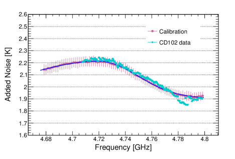
Figure 1: The average added noise obtained from the calibration (pink points) and the noise estimated from the CD102 data (light blue points) as a function of frequency. The error bars on the pink points are the RMS of $T_{\text{a}}$, as computed from the 19 measurements for each frequency in the calibration. The blue curve is obtained after performing a fit to the pink points and is used to estimate $T_{\text{a}}$ at the corresponding frequency.

IV Analysis Procedure

The goal of TASEH is to find the axion signal hidden in the noise. In order to achieve this, the analysis procedure includes the following steps:

1. Perform fast Fourier transform (FFT) on the IQ time series data to obtain the frequency-domain power spectrum.

2. Apply the Savitzky-Golay (SG) filter to remove the structure of the background in the frequency-domain power spectrum.

3. Combine all the spectra from different frequency scans with the weighting algorithm.

4. Merge bins in the combined spectrum to maximize the SNR.

5. Rescan the frequency regions with candidates and set limits on the axion-two-photon coupling $\left|g_{a\gamma\gamma}\right|$ if no candidates were found.

The analysis follows the procedure similar to that developed by the HAYSTAC experiment [45]. The important points and formulas for each step are highlighted below as a reminder for the convenience of readers. Note there are a few small differences between the HAYSTAC analysis and the one presented here. In this paper, the uncertainties are considered to be uncorrelated between different frequency bins while Ref. [45] takes into account the correlation. The frequency-domain spectra processed by each intermediate step are shown. The central results of the $\left|g_{a\gamma\gamma}\right|$ limits assume the signal line shape described by Eq. (4) as in Ref. [45]. In addition, the limits without an assumption of signal line shape and the limits assuming a Gaussian signal with a narrower FWHM are shown for comparison in Sec. VII. As a sanity check, the data are analyzed by two independent groups and their results are consistent with each other.

IV.1 Fast Fourier transform

The in-phase $I(t)$ and quadrature $Q(t)$ components of the time-domain data were sampled and saved in the TDMS (Technical Data Management Streaming) files - a binary format developed by National Instruments. The FFT is performed to convert the data into frequency-domain power spectrum in which the power is calculated using the following equation:

$$\text{Power}=\frac{|\text{FFT}(I+i\cdot Q)|^{2}}{N\cdot 2R},$$ (9)

where $N$ is the number of data points ($N=2000$ in the TASEH CD102 data), and $R$ is the input resistance of the signal analyzer (50 $\Omega$). The FFT is done for every one-millisecond subspectrum data. The integration time for each frequency scan was about 32-42 minutes, which resulted in 1920000 to 2520000 subspectra; an average over these subspectra gives the averaged frequency-domain power spectrum for each scan. The frequency span in the spectrum from each resonant-frequency scan is 2 MHz while the resolution is 1 kHz. In order to avoid the aliasing effect, a band-pass filter was applied in the data acquisition, giving a frequency span of 1.6 MHz (1600 frequency bins) that can be used for the analysis.

IV.2 Remove the structure of the background

In the absence of the axion signal, the output data spectrum is simply the noise from the cavity and the amplification chain. If axions are present in the cavity, the signal will be buried in the noise because the signal power is very weak. Therefore, the structure of the raw averaged output power spectrum, as shown in the upper left panel of Fig. 2, is dominated by the noise of the system and an explanation for the structure can be found in Appendix A. The SG filter [53], a digital filter that can smooth data without distorting the signal tendency, is applied to remove the structure of the background. The SG filter is performed on the averaged spectrum of each frequency scan by fitting adjacent points of successive sub-sets of data with an $n^{\text{th}}$-order polynomial. The result depends on two parameters: the number of data points used for fitting, the so-called window width, and the order of the polynomial. If the window is too wide, the filter will not remove small structures, and if it is too narrow, it may kill the signal. A window width of 201 frequency bins and a 4${}^{\text{th}}$-order polynomial were first chosen during the data taking, by requiring the ratio of the raw data to the filter output consistent with unity. The SG-filter parameters are also cross-checked using 10000 pseudo-experiments that include simulations of the noise spectrum and an axion signal with $\left|g_{a\gamma\gamma}\right|\approx 10\left|g_{a\gamma\gamma}^{\text{KSVZ}}\right|$; the measured signal power is found to be consistent with the injected one within 1%.

The SG-filter output can be considered as the averaged noise power. The raw averaged power spectrum is divided by the output of the SG filter, then unity is subtracted from the ratio to get the dimensionless normalized spectrum (lower left panel of Fig. 2). The relative deviation of power (RDP) in the normalized spectrum (and also in the spectra processed with rescaling, combining, and merging afterwards) are denoted by the symbol $\delta$. The values of RDPs can be zero, positive, or negative. In the absence of the axion signal, the RDPs in the normalized spectrum are samples drawn from a Gaussian distribution with a zero mean and a standard deviation of $\left.1\middle/\sqrt{N_{\text{spectra}}}\right.$, where $N_{\text{spectra}}$ is the number of subspectra used to compute the average (see Sec. IV.1 and the right panel of Fig. 2).

The normalized spectrum from each scan is further rescaled with the following formula:

$$\delta_{ij}^{\text{res}}=R_{ij}\delta_{ij}^{\text{norm}},$$ (10)

and the standard deviation of each bin is:

$$\sigma_{ij}^{\text{res}}=R_{ij}\sigma_{i}^{\text{norm}},$$ (11)

where

$$R_{ij}=\frac{k_{B}T_{\text{sys}}\Delta f_{\text{bin}}}{P_{ij}^{\text{KSVZ}}h_{ij}},$$ (12)

and

$$h_{ij}=\frac{1}{1+4Q_{Li}^{2}(\left.f_{ij}\middle/f_{ci}\right.-1)^{2}}.$$ (13)

The notations $\delta_{ij}^{\text{norm}}$ ($\delta_{ij}^{\text{res}}$) and $\sigma_{i}^{\text{norm}}$ ($\sigma_{ij}^{\text{res}}$) are the RDP and the standard deviation of the $j^{\text{th}}$ frequency bin in the normalized (rescaled) spectrum from the $i^{\text{th}}$ resonant-frequency scan. The value of $\sigma_{i}^{\text{norm}}$ is derived from the spread of the RDPs over the 1600 frequency bins for the $i^{\text{th}}$ scan (see an example in the right panel of Fig. 2). The factor $R_{ij}$ is the ratio of the system noise power to the expected signal power of the KSVZ axion $P_{ij}^{\text{KSVZ}}$, with the Lorentzian cavity response $h_{ij}$ taken into account. The system-noise temperature $T_{\text{sys}}$ in Eq. (12) is calculated following Eq. (6), where the frequency dependence of the added-noise temperature $T_{\text{a}}$ is obtained from the fitting function in Fig. 1. The symbol $\Delta f_{\text{bin}}$ is the bin width of spectrum (1 kHz). The factor $h_{ij}$ describes the Lorentzian response of the cavity, which depends on the loaded quality factor $Q_{Li}$ and the difference between the frequency $f_{ij}$ in bin $j$ and the resonant frequency $f_{ci}$. If a signal appears in a certain frequency bin $j$, its expected power will vary depending on the bin position due to the cavity’s Lorentzian response. The rescaling will take into account this effect. The procedure of the normalization and the rescaling also ensures that a KSVZ axion signal will have a rescaled RDP $\delta_{ij}^{\text{res}}$ that is approximately equal to unity, if the signal power is distributed in only one frequency bin.

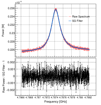
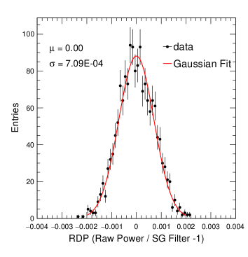
Figure 2: Upper left panel: The raw averaged power spectrum (red points) and the output of the SG filter (blue curve) of one scan. Lower left panel: The normalized spectrum, derived by taking the ratio of the raw spectrum to the SG filter and subtracting unity from the ratio. Right plot: Histogram of the normalized spectrum (lower panel in left plot) with a Gaussian fit; there are 1600 entries in total (from the 1600 frequency bins). The fitted mean and standard deviation are shown to be consistent with the prediction when the axion signal is not present.

IV.3 Combine the spectra with the weighting algorithm

During the data taking, the resonant frequency of the cavity was adjusted by the tuning bar to scan a large range of frequencies. Therefore, the spectra of all the scans need to be combined to create one big spectrum. The purpose of the weighting algorithm is to add the spectra from different resonant-frequency scans, particularly for the frequency bins that appear in multiple spectra. Note that the uncertainty of the averaged power at the overlapped region is reduced due to the combination. The weight is defined below:

$${w_{ijn}}=\frac{\Gamma_{ijn}}{(\sigma_{ij}^{\text{res}})^{2}}.$$ (14)

Here, the symbol $\Gamma_{ijn}=1$ if the $j^{\text{th}}$ frequency bin in the $i^{\text{th}}$ rescaled spectrum correspond to the same frequency in the $n^{\text{th}}$ bin of the combined spectrum; otherwise, $\Gamma_{ijn}=0$.

The RDP $\delta^{\text{com}}_{n}$ and the standard deviation $\sigma^{\text{com}}_{n}$ of the $n^{\text{th}}$ bin in the combined spectrum are calculated using Eq. (15) and Eq. (16), respectively. The notation SNR${}^{\text{com}}_{n}$ is the ratio of $\delta^{\text{com}}_{n}$ to $\sigma^{\text{com}}_{n}$ as given in Eq. (17). Figure 3 shows the SNR of the combined spectrum.

$$\delta_{n}^{\text{com}}=\frac{\sum\limits_{i}\sum\limits_{j}\left(\delta_{ij}^{\text{res}}\cdot{w_{ijn}}\right)}{\sum\limits_{i}\sum\limits_{j}{w_{ijn}}},$$ (15)

$$\sigma_{n}^{\text{com}}=\frac{\sqrt{\sum\limits_{i}\sum\limits_{j}(\sigma_{ij}^{\text{res}}\cdot{w_{ijn}})^{2}}}{\sum\limits_{i}\sum\limits_{j}{w_{ijn}}},$$ (16)

$$\text{SNR}_{n}^{\text{com}}=\frac{\delta^{\text{com}}_{n}}{\sigma^{\text{com}}_{n}}=\frac{\sum\limits_{i}\sum\limits_{j}\left(\delta_{ij}^{\text{res}}\cdot{w_{ijn}}\right)}{\sqrt{\sum\limits_{i}\sum\limits_{j}(\sigma_{ij}^{\text{res}}\cdot{w_{ijn}})^{2}}}.$$ (17)

The summations over $i$ run from 1 to 837 (steps) while the summations over $j$ run from 1 to 1600 (bins). For each bin $n$ in the combined spectrum, there are $m_{n}$ non-vanishing contributions to the sums above. In general, the value of $m_{n}$ is 14–16.

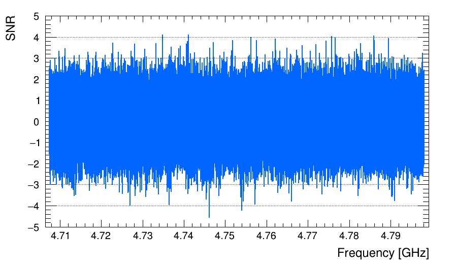
Figure 3: The signal-to-noise ratio (SNR) calculated using Eq.(17) of the combined spectrum.

IV.4 Merge bins

The expected axion bandwidth is about 5 kHz at the frequency of $\approx 5$ GHz. In this paper, the interested frequency range is 4.70750 – 4.79815 GHz and the bin width is 1 kHz. Therefore, in order to maximize the SNR, a running window of five consecutive bins in the combined spectrum is applied and the five bins within each window are merged to construct a final spectrum. The purpose of using a running window is to avoid the signal power broken into different neighboring bins of the merged spectrum. The number of bins for merging is studied by injecting simulated axion signals on top of the CD102 data and optimized based on the SNR.

Due to the nonuniform distribution of the axion signal [Eq. (4)], the contributing bins need to be rescaled to have the same RDP, of which the standard deviation is used to define the maximum likelihood (ML) weight for merging. The rescaling is performed by dividing the values of $\delta^{\text{com}}_{g+k-1}$ and $\sigma^{\text{com}}_{g+k-1}$ in the combined spectrum with an integral of the signal line shape $L_{k}$:

$$L_{k}=\int_{f_{a}+\delta f_{m}+(k-1)\Delta f_{\text{bin}}}^{f_{a}+\delta f_{m}+k\Delta f_{\text{bin}}}\mathcal{F}(f,f_{a})\,df,$$ (18)

where the variable $g$ is the index for the frequency bins in the final merged spectrum and $k$ is the index within the group of bins for merging. The index $g$ runs from 1 to $N-M+1$, where the number $N$ is the total number of bins in the combined spectrum and $M=5$ is the number of merged bin in this analysis. The frequency $f_{a}=\left.m_{a}c^{2}\middle/h\right.$ is the axion frequency, and $\delta f_{m}$ is the misalignment between $f_{a}$ and the lower boundary of the $g^{\text{th}}$ bin in the merged spectrum. The function $\mathcal{F}(f,f_{a})$ has been defined in Eq. (4). In order to get a misalignment-independent line shape, instead of using an $L_{k}$ that depends on the frequency $f_{a}$ and $\delta f_{m}$, the average ($\bar{L}_{k}$) of $L_{k}$ over the ranges of $f_{a}$ and $\delta f_{m}$ is used. Note that the relative variation of $f_{a}$ is at most 90 MHz/5 GHz$\approx 2\%$ and the line shape of $\mathcal{F}(f,f_{a})$ can be considered constant for the full range of the operational frequency. Therefore, the value of $L_{k}$ has only weak dependence on $f_{a}$. In the analysis presented here, $\bar{L}_{k}=0.23,0.33,0.21,0.11,0.06$ for $k=1,...5$, respectively. The effect of the misalignment on the $\left|g_{a\gamma\gamma}\right|$ limits is quoted as a part of the systematic uncertainty using the same method as described in the HAYSTAC paper [45], see Sec. VI.

The rescaled RDP $\delta^{\text{rs}}_{g+k-1}$ and standard deviation $\sigma^{\text{rs}}_{g+k-1}$ are calculated:

$$\begin{split}\delta^{\text{rs}}_{g+k-1}=\frac{\delta^{\text{com}}_{g+k-1}}{\bar{L}_{k}},\\ \sigma^{\text{rs}}_{g+k-1}=\frac{\sigma^{\text{com}}_{g+k-1}}{\bar{L}_{k}}.\end{split}$$ (19)

After this rescaling procedure, a KSVZ axion signal is expected to have an RDP equal to unity for each of the five bins. The ML weight is defined as:

$$w_{gk}=\frac{1}{(\sigma_{g+k-1}^{\text{rs}})^{2}}=\frac{\bar{L}_{k}^{2}}{(\sigma_{g+k-1}^{\text{com}})^{2}}.$$ (20)

The RDP, the standard deviation, and the SNR of the merged spectrum are:

$$\delta_{g}^{\text{merged}}=\frac{\sum\limits_{k=1}^{M}\left(\delta_{g+k-1}^{\text{rs}}\cdot{w_{gk}}\right)}{\sum\limits_{k=1}^{M}{w_{gk}}}=\frac{\sum\limits_{k=1}^{M}\frac{\delta_{g+k-1}^{\text{com}}}{\bar{L}_{k}}\cdot\left(\frac{\bar{L}_{k}}{\sigma_{g+k-1}^{\text{com}}}\right)^{2}}{\sum\limits_{k=1}^{M}\left(\frac{\bar{L}_{k}}{\sigma_{g+k-1}^{\text{com}}}\right)^{2}},$$ (21)

$$\sigma_{g}^{\text{merged}} = \frac{\sqrt{\sum\limits_{k=1}^{M}\left(\sigma_{g+k-1}^{\text{rs}}\cdot{w_{gk}}\right)^{2}}}{\sum\limits_{k=1}^{M}{w_{gk}}}=\frac{\sqrt{\sum\limits_{k=1}^{M}\left(\frac{\bar{L}_{k}}{\sigma_{g+k-1}^{\text{com}}}\right)^{2}}}{\sum\limits_{k=1}^{M}\left(\frac{\bar{L}_{k}}{\sigma_{g+k-1}^{\text{com}}}\right)^{2}}$$ (22)

$$= \frac{1}{\sqrt{\sum\limits_{k=1}^{M}\left(\frac{\bar{L}_{k}}{\sigma_{g+k-1}^{\text{com}}}\right)^{2}}}$$

$$\text{SNR}_{g}^{\text{merged}}=\frac{\delta^{\text{merged}}_{g}}{\sigma^{\text{merged}}_{g}}=\frac{\sum\limits_{k=1}^{M}\frac{\delta_{g+k-1}^{\text{com}}}{\bar{L}_{k}}\cdot\left(\frac{\bar{L}_{k}}{\sigma_{g+k-1}^{\text{com}}}\right)^{2}}{\sqrt{\sum\limits_{k=1}^{M}\left(\frac{\bar{L}_{k}}{\sigma_{g+k-1}^{\text{com}}}\right)^{2}}}$$ (23)

IV.5 Rescan and set limits on $\left|g_{a\gamma\gamma}\right|$

Before the collection of the CD102 data, a 5$\sigma$ SNR target was chosen, which corresponds to a candidate threshold of 3.355$\sigma$ at 95% C.L.. After the merging as described in Sec. IV.4, if there were any potential signal with an SNR larger than 3.355, a rescan would be proceeded to check if it were a real signal or a statistical fluctuation. The procedure of the CD102 data taking was to perform a rescan after covering every 10 MHz; the rescan was done by adjusting the tuning rod of the cavity so to match the resonant frequency to the frequency of the candidate. In total, 22 candidates with an SNR greater than 3.355 were found. Among them, 20 candidates were from the fluctuations because they were gone after a few rescans. The remaining two candidates, in the frequency ranges of 4.71017 – 4.71019 GHz and 4.74730 – 4.74738 GHz, are excluded from consideration of axion signal candidates due to the following reasons. The signal in the second frequency range was detected via a portable antenna outside the DR and found to come from the instrument control computer in the laboratory, while the signal in the first frequency range was not detected outside the DR but still present after turning off the external magnetic field. No limits are placed for the two frequency ranges above. More details can be found in the TASEH instrumentation paper [52]. Figure 4 shows the SNR of the merged spectrum after including data from both the original scans and the rescans.

Since no candidates were found after the rescan, an upper limit on the signal power $P_{s}$ is derived by setting $P_{s}$ equal to $5\sigma_{g}^{\text{merged}}\times P_{g}^{\text{KSVZ}}$, where $\sigma_{g}^{\text{merged}}$ is the standard deviation and $P_{g}^{\text{KSVZ}}$ is the expected signal power for the KSVZ axion for a certain frequency bin $g$ in the merged spectrum. Then, the 95% C.L. limits on the axion-two-photon coupling $\left|g_{a\gamma\gamma}\right|$ could be derived according to Eq. (2). See Sec. VII for the final limits including the systematic uncertainties.

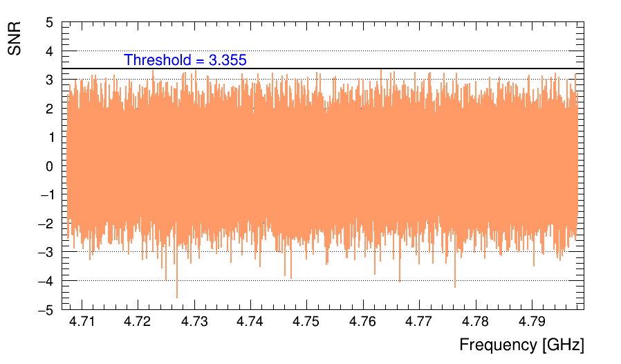
Figure 4: The signal-to-noise ratio (SNR) calculated using Eq. (23) for the merged spectrum including data from both the original scans and the rescans. No candidate exceeds the threshold of $3.355\sigma$ (solid-black horizontal line).

V Analysis of the Synthetic Axion Data

After TASEH finished collecting the CD102 data on November 15, 2021, the synthetic axion signals were injected into the cavity and read out via the same transmission line and amplification chain. The procedure to generate axion-like signals is summarized in Ref. [52]. A test with synthetic axion signals could be used to verify the procedures of data acquisition and physics analysis. The synthetic axion signals have a wider width (8 kHz) and longer tails compared to the line shape described by Eq. (4). The expected SNR of the frequency bin with maximum power ($\approx 11\%$ of the total signal power), at 4.70897 GHz, was set to $\approx 3.35$. The total signal power injected corresponds to $\left|g_{a\gamma\gamma}\right|\approx 20\left|g_{a\gamma\gamma}^{\text{KSVZ}}\right|$.

The same analysis procedure as described in Sec. IV is applied to the data with synthetic axion signals. Figure 5 presents the individual raw power spectra in the 24 frequency scans. Before combining the 24 spectra, the SNR of the maximum-power bin from the scan with a resonant frequency closest to the injected signal is measured to be 3.58. After the combination of the spectra and the merging of five frequency bins, the SNRs of the maximum-power bin increase to 4.74 and 6.12, respectively. Figure 6 presents the SNR after the combination and the merging, respectively. In order to validate the results of the SNRs, the analysis procedure is also applied to the simulated spectra that include both noise and a signal with the same power and the same line shape as those of the injected synthetic axions. The SNRs obtained with 200 simulations, before the combining, after the combining, and after the merging are $3.6\pm 0.5$, $4.5\pm 0.6$, and $6.9\pm 0.8$, respectively, which are consistent with the results from the synthetic axion data. The consistency of the SNRs demonstrates the capability of the TASEH apparatus and the analysis procedure to discover an axion signal with $\left|g_{a\gamma\gamma}\right|\approx{\cal O}\left(10\left|g_{a\gamma\gamma}^{\text{KSVZ}}\right|\right)$.

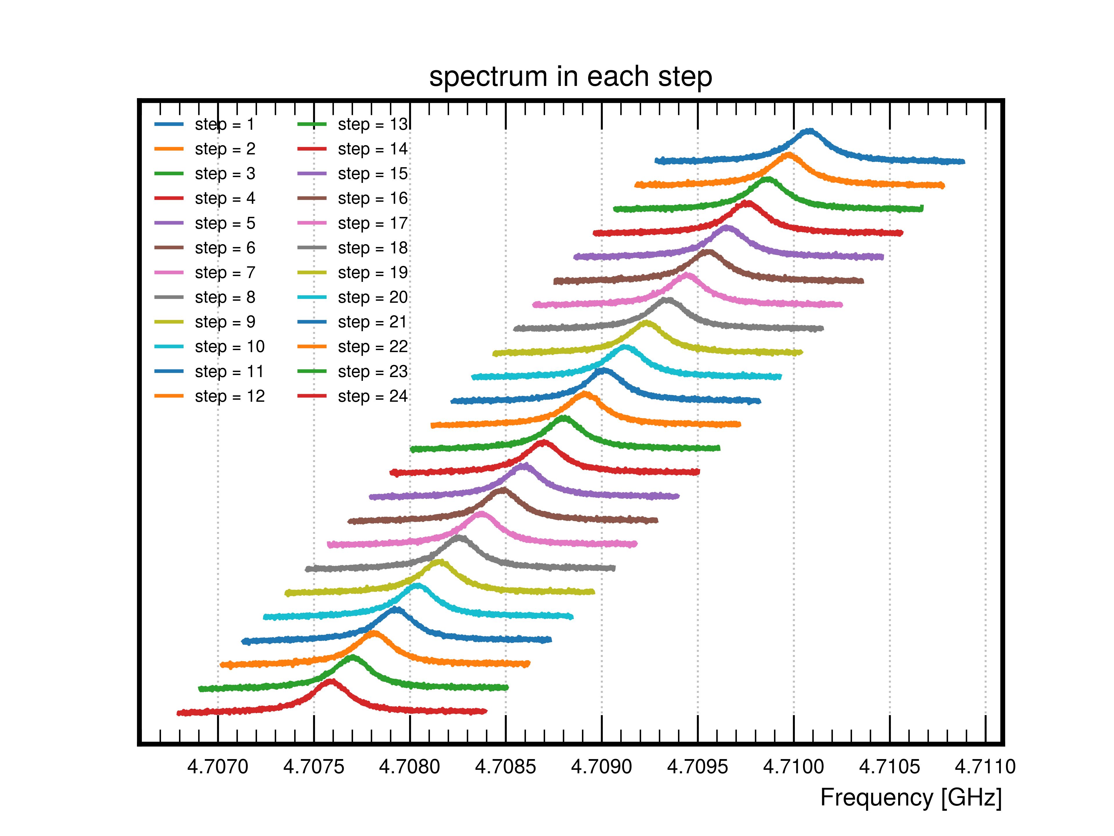
Figure 5: The raw output power spectra, before applying the SG filter, from the 24 frequency steps of the synthetic axion data. In order to show the spectra clearly, the spectra are shifted with respect to each other with an arbitrary offset in the vertical scale.

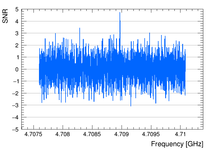
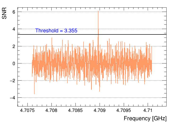
Figure 6: The signal-to-noise ratio, from the synthetic axion data, after combining the spectra with overlapping frequencies from different scans (upper) and after merging the RDP measured in five neighboring frequency bins (lower). The procedure and the weights for combination and merging are summarized in Sec. IV.3 and Sec. IV.4, respectively.

VI Systematic Uncertainties

The systematic uncertainties on the $\left|g_{a\gamma\gamma}\right|$ limits arise from the following sources:

• Uncertainty on the product $\left.Q_{L}\beta\middle/\left(1+\beta\right)\right.$ in Eq. (2): In order to extract the loaded quality factor $Q_{L}$ and the coupling coefficient $\beta$, a fitting of the measured results of the cavity scattering matrix was performed. A relative uncertainty of 3.6% is assigned to this product, after a comparison of the measurements at $T_{\text{c}}\simeq 155$ mK with a prediction rescaled from the measurements at room temperature. More details about the measurements of the cavity properties can be found in Ref. [52]. A 3.6% variation of this product results in a 1.9% uncertainty on the $\left|g_{a\gamma\gamma}\right|$ limits.

• Uncertainty on the form factor $C_{010}$: the variation of $C_{010}$, due to the different grid sizes in the integrals of Eq. (3), is within 1%, which gives a $\leq 0.5$% uncertainty on the $\left|g_{a\gamma\gamma}\right|$ limits.

• Uncertainties on the noise temperature $T_{\text{a}}$ from: (i) the RMS of the measurements in the calibration: $\left.\Delta T_{\text{a}}\middle/T_{\text{a}}\right.=2.3\%$, and (ii) from the largest difference between the value determined by the calibration and that from the CD102 data: $\left.\Delta T_{\text{a}}\middle/T_{\text{a}}\right.=4\%$ (see Sec. III and Fig. 1). These two uncertainties on $T_{\text{a}}$ result in a 2.8% uncertainty on the $\left|g_{a\gamma\gamma}\right|$ limits.

• Uncertainty due to the misalignment (see Sec. IV.4): estimated by comparing the central results to the one without misalignment ($\delta f_{m}=0$) and to the ones with given values of $\delta f_{m}$. The comparison shows that $\delta f_{m}=0$ gives the largest difference of 2.8% on the limit, which is used as the systematic uncertainty from the misalignment.

• Uncertainty from the choice of the SG-filter parameters: i.e. the window width and the order of the polynomial in the SG filter. At the beginning of the data taking, a preliminary optimization was performed: a window width of 201 bins and a 4${}^{\text{th}}$-order polynomial were used for the first analysis of the CD102 data (see Sec. IV). This choice is kept for the central results. Nevertheless, various methods of optimization are also explored. The goal of the optimization is to find a set of SG-filter parameters that only model the noise spectrum and do not remove a real signal. The methods include:

  • Minimize the difference between the two outputs returned by the SG filter, when the SG filter is applied to: (i) the real data only, and (ii) the sum of the real data and the simulated axion signals.

  • Minimize the difference between the output returned by the SG filter and the function ${\cal G}_{\text{noise}}$ that models the noise spectrum (derived by fitting the CD102 data), when the SG filter is applied to the sum of the simulated noise based on ${\cal G}_{\text{noise}}$ and the simulated axion signals. See Fig. 7 for an example of the simulated spectrum, the function ${\cal G}_{\text{noise}}$, and the output returned by the SG filter when a 3${}^{\text{rd}}$-order polynomial and a window of 141 bins are chosen; the squared differences from all the frequency bins are summed together (rescaled $\chi^{2}$) when performing the optimization. Figure 8 shows the rescaled $\chi^{2}$ as a function of window widths when the order of polynomial is set to three, four, and six.

  • Compare the mean $\mu_{\text{noise}}$ and the width $\sigma_{\text{noise}}$ of the measured power after applying the SG filter, assuming that no signal is present in the data. See Fig. 9 for an example distribution of the measured power from the averaged spectrum of a single scan; a Gaussian fit is performed to extract $\mu_{\text{noise}}$ and $\sigma_{\text{noise}}$. Given the nature of the thermal noise [51], the two variables are supposed to be related to each other if a proper window width and a proper order are chosen:

    $$\sigma_{\text{noise}}=\frac{\mu_{\text{noise}}}{\sqrt{N_{\text{spectra}}}},$$

    where $N_{\text{spectra}}$ is the number of spectra for averaging and is related to the amount of integration time for each frequency step. In general, $N_{\text{spectra}}=1920000-2520000$.

  In addition, one could choose to optimize for each frequency step individually, optimize for a certain frequency step but apply the results to all data, or optimize by fitting together the spectra from all the frequency steps. The deviations from the central results using different optimization approaches are in general within 1% and the maximum deviation of 1.8% on the $\left|g_{a\gamma\gamma}\right|$ limit is used as a conservative estimate of the systematic uncertainty from the SG filter.

The effects on the $\left|g_{a\gamma\gamma}\right|$ limits from these sources are studied and added in quadrature to obtain the total systematic uncertainty. The systematic uncertainties on the $\left|g_{a\gamma\gamma}\right|$ limits are displayed together with the central results in Sec. VII. Overall the total relative systematic uncertainty is $\approx 4.6\%$.

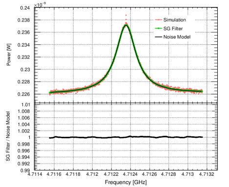
Figure 7: Upper panel: The simulated spectrum (red), including the axion signal and the noise, is overlaid with the function that models the noise ${\cal G}_{\text{noise}}$ (black) and the output returned by the SG filter (green). Lower panel: The ratio of the output returned by the SG filter to the function ${\cal G}_{\text{noise}}$.

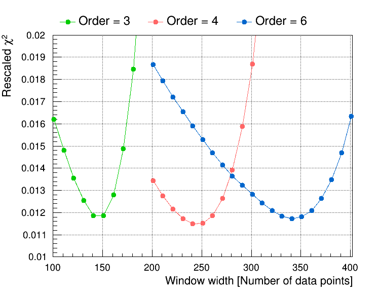
Figure 8: The rescaled $\chi^{2}$ when various values of window widths and a 3${}^{\text{rd}}$, a 4${}^{\text{th}}$, or a 6${}^{\text{th}}$-order polynomial are applied in the SG filter. The rescaled $\chi^{2}$ is defined as the sum of the squared differences from all the frequency bins, between the output returned by the SG filter and the function that models the noise spectrum ${\cal G}_{\text{noise}}$ (see Fig. 7). In this figure, the best choice is a 4${}^{\text{th}}$-order polynomial with a window width of 241 data points (bins).

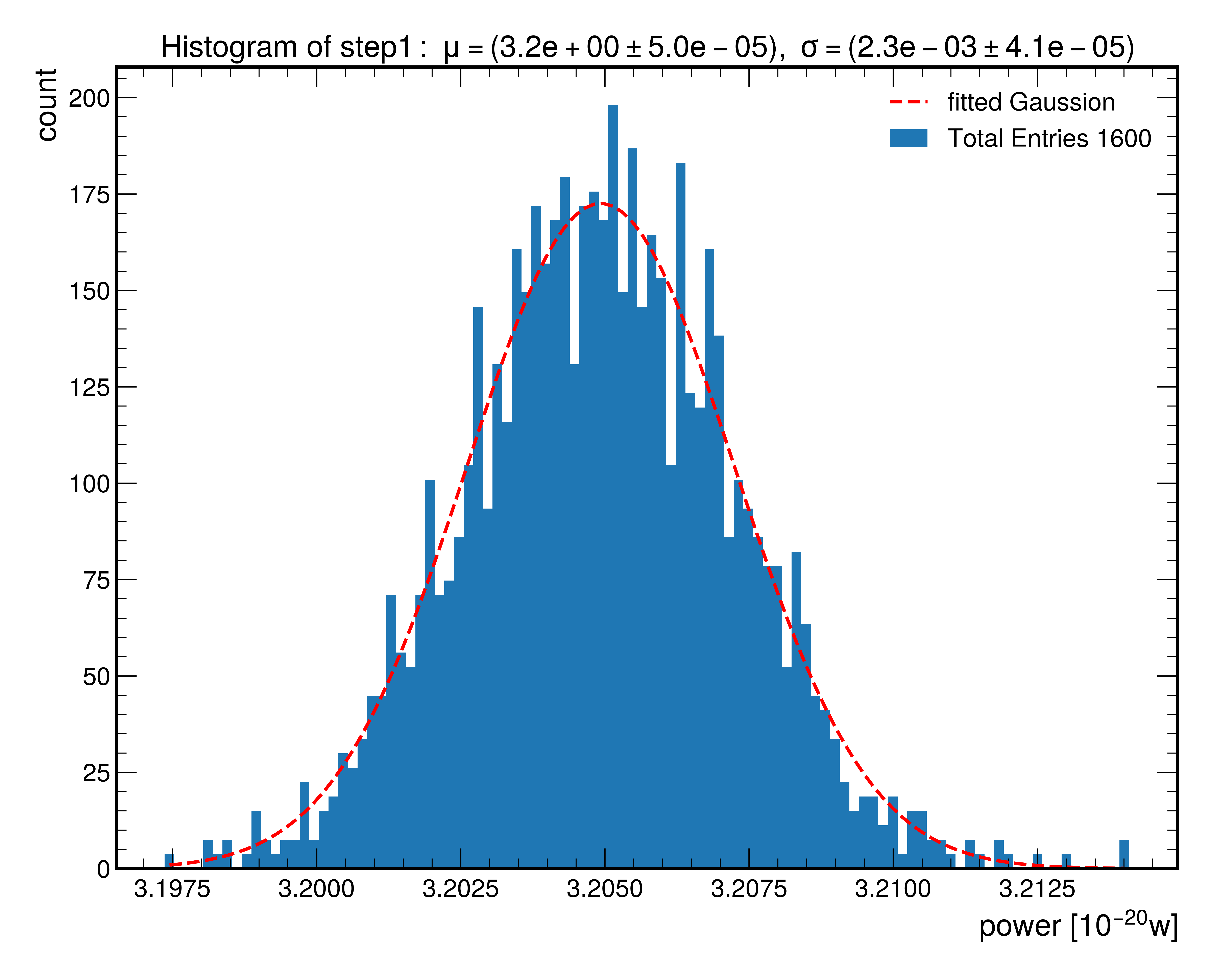
Figure 9: An example of the distribution of the measured power after applying the SG filter, when the cavity resonant frequency is 4.79815 GHz. The distribution contains 1600 entries and each entry corresponds to the measured power in one frequency bin, averaged over 1920000 subspectra. The mean and the width returned by a Gaussian fit to the distribution are used to determine the best choice of SG parameters. The fitted Gaussian mean $\mu$ divided by $\sqrt{1920000}$ is consistent with the fitted Gaussian width $\sigma$. The best choice of SG parameters obtained for this scan is a window of 189 data points (bins) with a 3${}^{\text{rd}}$-order polynomial.

VII Results

Figure 10 shows the 95% C.L. limits on $\left|g_{a\gamma\gamma}\right|$ and the ratio of the limits with respect to the KSVZ benchmark value. The blue error band indicates the systematic uncertainties as discussed in Sec. VI. Note the uncertainties here are solely due to the variations in the experimental parameters and in the analysis procedure of TASEH. The uncertainties on the local dark matter density $\rho_{a}$, which can be as large as 50%, are considered external uncertainties and not included in the blue error band. No limits are placed for the frequency ranges 4.71017 – 4.71019 GHz and 4.74730 – 4.74738 GHz, corresponding to the regions in which non-axion signals were observed during the collection of the CD102 data. The limits on $\left|g_{a\gamma\gamma}\right|$ range from $5.3\times 10^{-14}\,\text{GeV}^{-1}$ to $8.9\times 10^{-14}\,\text{GeV}^{-1}$, with an average value of $8.2\times 10^{-14}\,\text{GeV}^{-1}$; the lowest value comes from the frequency bins with additional eight times more data from the rescans, while the highest value comes from the frequency bins near the boundaries of the spectrum. Figure 11 displays the $\left|g_{a\gamma\gamma}\right|$ limits obtained by TASEH together with those from the previous searches. The results of TASEH exclude the models with the axion-two-photon coupling $\left|g_{a\gamma\gamma}\right|\gtrsim 8.2\times 10^{-14}\,\text{GeV}^{-1}$, a factor of eleven above the benchmark KSVZ model for the mass range $19.4687<m_{a}<19.8436\,\mu\text{eV}$ (corresponding to the frequency range of $4.70750<f_{a}<4.79815$ GHz).

The central results in Figs. 10–11 are obtained assuming an axion signal line shape that follows Eq. (4). The $\left|g_{a\gamma\gamma}\right|$ limits from the analysis that merges frequency bins without assuming a signal line shape are $\approx 5.5$% larger than the central values. If a Gaussian signal line shape with an FWHM of 2.5 kHz, about half of the axion line width in Eq. (4), is assumed instead, the limits will be $\approx 3.8$% smaller than the central results. If the $\left|g_{a\gamma\gamma}\right|$ limits are derived from the observed SNR as described in the ADMX paper [54], rather than using the 5$\sigma$ target SNR, the average limit on $\left|g_{a\gamma\gamma}\right|$ will be $\approx 4.9\times 10^{-14}\,\text{GeV}^{-1}$.

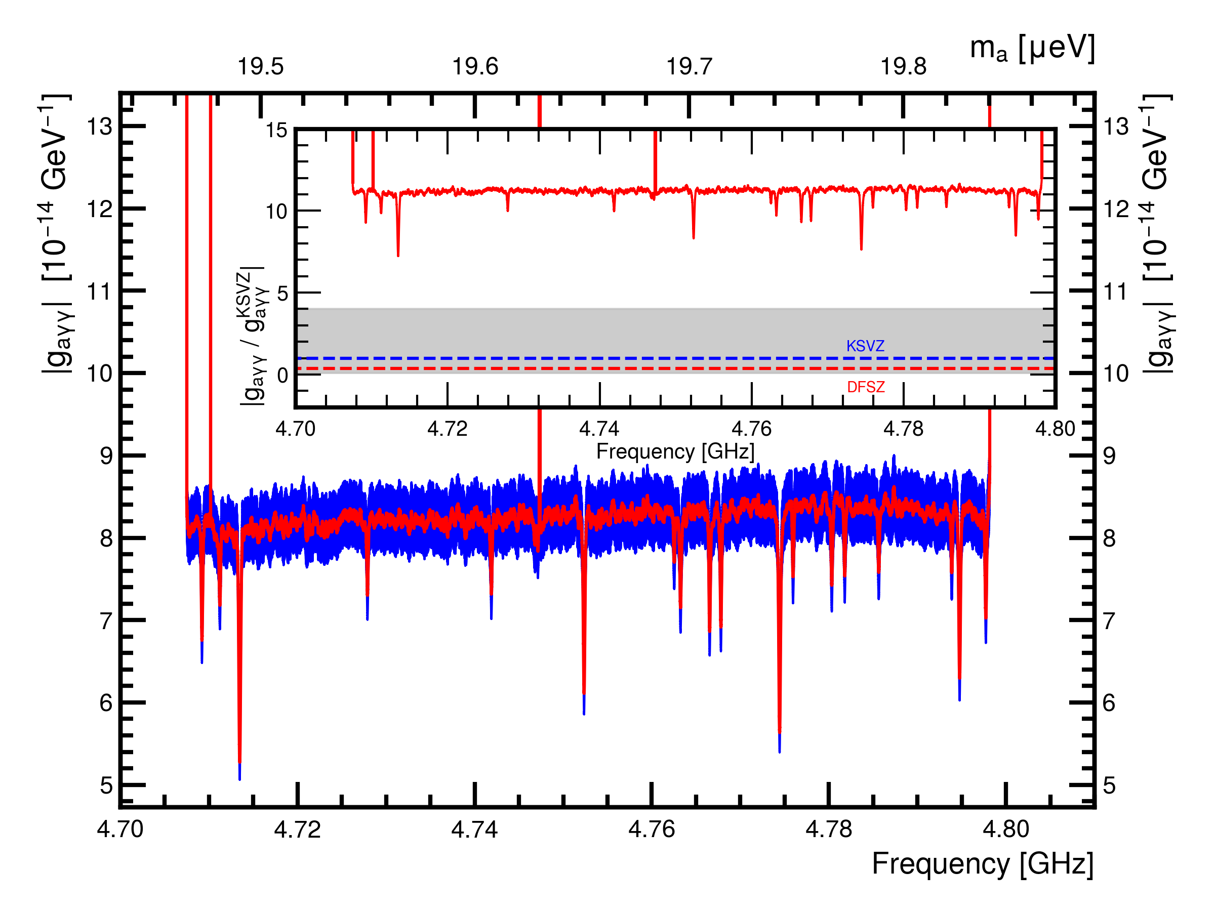
Figure 10: The 95% C.L. limits on $\left|g_{a\gamma\gamma}\right|$ and the ratio of the limits relative to the KSVZ benchmark value (inset), for the frequency range of 4.70750–4.79815 GHz. The blue error band indicates the systematic uncertainties as discussed in Sec. VI. The gray band in the inset shows the allowed region of $\left|g_{a\gamma\gamma}\right|$ vs. $m_{a}$ from various QCD axion models, while the blue and red dashed lines are the values predicted by the KSVZ and DFSZ benchmark models, respectively.

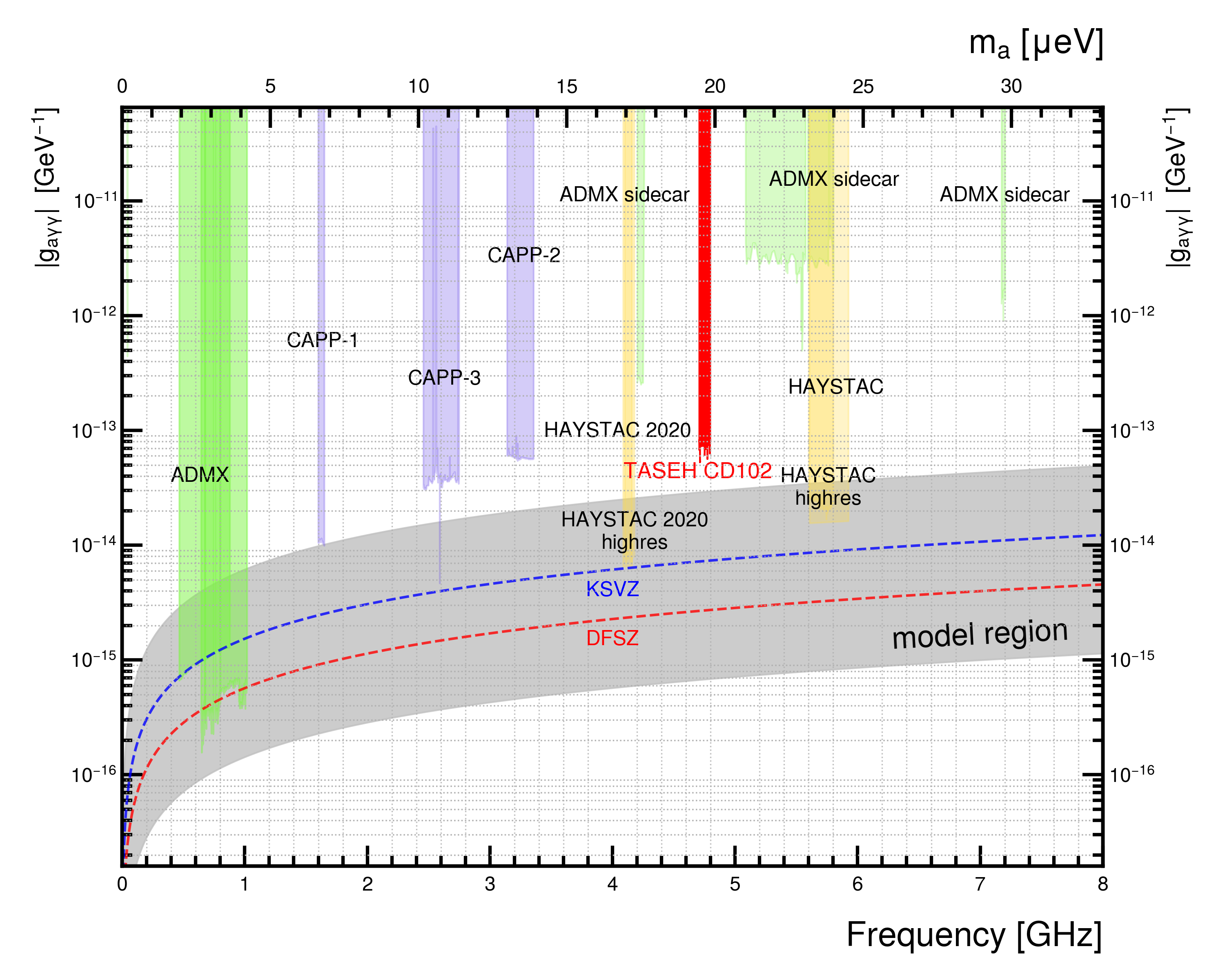
Figure 11: The limits on the axion-two-photon coupling $\left|g_{a\gamma\gamma}\right|$ for the frequency range 0–8 GHz, from the CD102 data of TASEH (red band) and previous searches performed by the ADMX, CAPP, and HAYSTAC Collaborations. The gray band indicates the allowed region of $\left|g_{a\gamma\gamma}\right|$ vs. $m_{a}$ from various QCD axion models while the blue and red dashed lines are the values predicted by the KSVZ and DFSZ benchmark models, respectively.

VIII Conclusion

This paper presents the analysis details of a search for axions for the mass range $19.4687<m_{a}<19.8436\,\mu\text{eV}$, using the CD102 data collected by the Taiwan Axion Search Experiment with Haloscope from October 13, 2021 to November 15, 2021. Apart from the non-axion signals, no candidates with a significance more than 3.355 were found. The synthetic axion signals were injected after the collection of data and the successful results validate the data acquisition and the analysis procedure.

The experiment excludes models with the axion-two-photon coupling $\left|g_{a\gamma\gamma}\right|\gtrsim 8.2\times 10^{-14}\,\text{GeV}^{-1}$ at 95% C.L., a factor of eleven above the benchmark KSVZ model. The sensitivity on $\left|g_{a\gamma\gamma}\right|$ reached by TASEH is three orders of magnitude better than the existing limits in the same mass range. It is also the first time that a haloscope-type experiment places constraints in this mass region. The readers shall be aware that haloscope experiments assume that 100% of the dark matter is the axion. In addition, the local dark matter density, which is used to compute the expected axion signal power, can have an uncertainty as large as 50%; this uncertainty is typically considered an external uncertainty and not included in the experimental results.

The target of TASEH is to search for axions for the mass range of 16.5–20.7$\,\mu\text{eV}$ corresponding to a frequency range of 4–5 GHz, with a capability to be extended to 2.5–6 GHz in the future. In the coming years, several upgrades are expected, including: the use of a quantum-limited Josephson parametric amplifier as the first-stage amplifier, the replacement of the existing dilution refrigerator with a new one that has a magnetic field of about 9 Tesla and a larger bore size, and the development of a new cavity with a significantly larger effective volume. With the improvements of the experimental setup and several years of data taking, TASEH is expected to probe the QCD axion band in the target mass range.

Appendix A Derivation of the Function that Models the Noise Spectrum

The background noise from a cavity is governed by the thermal noise and the vacuum fluctuation. According to Planck’s law in one dimension (1D), the spectral density of the electromagnetic noise from the cavity, thermalized with an environment of temperature $T_{\rm c}$, through a transmission line is

$$S(\omega)=\hbar\omega\left(\frac{1}{e^{\hbar\omega/k_{\rm B}T_{\rm c}}-1}+\frac{1}{2}\right),$$ (24)

where $\omega$ is the angular frequency, $\hbar$ is the reduced Planck’s constant, and $k_{\rm B}$ is the Boltzmann constant.

However, the cavity body (the materials that form the cavity itself) may not be thermalized with its 1D electromagnetic environment. To understand the noise spectrum from the cavity near its resonant frequency $\omega_{\rm c}/2\pi$ in this scenario, the model in Fig. 12 is considered. Through a probe the cavity field mode $c$ is coupled to the modes $a_{2}$ of a 1D transmission line, representing the path toward a signal receiver, with a rate $\kappa_{2}$. The cavity field is also coupled to the modes of the cavity body $a_{0}$, representing the intrinsic loss, with a rate $\kappa_{0}$. In a steady state, the quantum input-output theory leads to a relation between the outgoing field from the cavity to the 1D transmission line, $a_{\rm 2,out}$, and the incoming fields, $a_{\rm 2,in}$ and $a_{\rm 0,in}$, through the elements of the cavity scattering matrix:

$$a_{\rm 2,out}=S^{*}_{\rm 22}a_{\rm 2,in}+S^{*}_{\rm 20}a_{\rm 0,in},$$ (25)

where $S_{\rm 22}=\frac{\kappa_{0}-\kappa_{\rm 2}+i2\Delta}{\kappa_{0}+\kappa_{\rm 2}+i2\Delta}$, $S_{\rm 20}=\frac{2\sqrt{\kappa_{0}\kappa_{\rm 2}}}{\kappa_{0}+\kappa_{\rm 2}+i2\Delta}$, and $\Delta=\omega-\omega_{\rm c}$ is the detuning.

As both incoming fields are in a thermal state, $\langle a_{i,\rm in}(0)a_{i,\rm in}(\tau)\rangle=n_{\rm th}(T_{i})\delta(\tau)$, where $n_{\rm th}(T_{i})=\frac{1}{e^{\hbar\omega/k_{\rm B}T_{i}}-1}$ is the mean thermal photon number of the incoming field $a_{i,\rm in}$ at the temperature $T_{i}$, and $\delta(\tau)$ is the $\delta$-function. In the model the incoming field $a_{\rm 2,in}$ comes from a nearby attenuator, anchored to the mixing flange, in the transmission line with a temperature $T_{\text{m}x}\equiv T_{\rm 2}$, and $a_{\rm 0,in}$ comes from the cavity body with a temperature $T_{\text{c}}\equiv T_{\rm 0}$.

By defining the effective temperature $\tilde{T}_{i}=\left(n_{\rm th}(T_{i})+\frac{1}{2}\right)\hbar\omega/k_{\rm B}$, the power spectral density of the outgoing field of the transmission line modes is

$$S_{\rm out}(\omega)= \int_{-\infty}^{\infty}\hbar\omega\left(\langle a_{2,\rm out}(0)a_{2,\rm out}(\tau)\rangle+\frac{1}{2}\right)e^{-i\omega\tau}d\tau$$ (26)

$$= |S_{\rm 22}|^{2}k_{\rm B}\tilde{T}_{2}+|S_{\rm 20}|^{2}k_{\rm B}\tilde{T}_{0}.$$

The total output noise can be viewed as the sum of the reflection of the incoming noise from the attenuator and the transmission of the noise from the cavity body itself. Via the unitary property of the cavity scattering matrix, i.e. $|S_{\rm 22}|^{2}+|S_{\rm 20}|^{2}=1$,

$$S_{\rm out}(\omega)=k_{\rm B}\tilde{T}_{2}+k_{\rm B}(\tilde{T}_{0}-\tilde{T}_{2})L(\omega),$$ (27)

where $L(\omega)=|S_{\rm 20}|^{2}=\frac{\kappa_{0}\kappa_{\rm 2}}{(\kappa_{0}+\kappa_{\rm 2})^{2}/4+\Delta^{2}}$ is a Lorentzian function with a FWHM $\kappa_{0}+\kappa_{\rm 2}$. Therefore, the noise spectrum has a flat background determined by the incoming noise of the attenuator with an effective temperature $\tilde{T}_{\rm 2}$, plus an excess Lorentzian peak centered at $\omega_{\rm c}$ determined by the effective temperature difference $\tilde{T}_{\rm 0}-\tilde{T}_{\rm 2}$. (The center Lorentzian structure can even be a dip if ${T}_{\rm 0}<{T}_{\rm 2}$.)

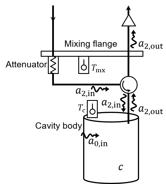
Figure 12: The input-output model of cavities. The cavity field mode $c$ is coupled to the modes of a 1D transmission line $a_{2}$ (with a rate $\kappa_{2}$) and the modes of the cavity body $a_{0}$ (with a rate $\kappa_{0}$). The incoming and outgoing fields of the transmission line are separated by the circulator. The attenuator and the cavity body emitting the fields $a_{2,\rm in}$ and $a_{0,\rm in}$ are thermalized at $T_{\rm mx}$ and $T_{\rm c}$, respectively.

References

- Peccei and Quinn [1977] R. D. Peccei and H. R. Quinn, Phys. Rev. Lett. 38, 1440 (1977).
- Weinberg [1978] S. Weinberg, Phys. Rev. Lett. 40, 223 (1978).
- Wilczek [1978] F. Wilczek, Phys. Rev. Lett. 40, 279 (1978).
- Abel et al. [2020] C. Abel et al. (nEDM), Phys. Rev. Lett. 124, 081803 (2020).
- Zyla et al. [2021] P. A. Zyla et al. (Particle Data Group), PTEP 2020, 083C01 (2021).
- Preskill et al. [1983] J. Preskill, M. B. Wise, and F. Wilczek, Physics Letters B 120, 127 (1983).
- Abbott and Sikivie [1983] L. Abbott and P. Sikivie, Physics Letters B 120, 133 (1983).
- Dine and Fischler [1983] M. Dine and W. Fischler, Physics Letters B 120, 137 (1983).
- Ipser and Sikivie [1983] J. Ipser and P. Sikivie, Phys. Rev. Lett. 50, 925 (1983).
- Borsanyi et al. [2016] S. Borsanyi, Z. Fodor, J. Guenther, K.-H. Kampert, S. D. Katz, T. Kawanai, T. G. Kovacs, S. W. Mages, A. Pasztor, F. Pittler, J. Redondo, A. Ringwald, and K. K. Szabo, Nature 539, 69 (2016).
- Dine et al. [2017] M. Dine, P. Draper, L. Stephenson-Haskins, and D. Xu, Phys. Rev. D 96, 095001 (2017).
- Hiramatsu et al. [2011] T. Hiramatsu, M. Kawasaki, T. Sekiguchi, M. Yamaguchi, and J. Yokoyama, Phys. Rev. D 83, 123531 (2011).
- Kawasaki et al. [2015] M. Kawasaki, K. Saikawa, and T. Sekiguchi, Phys. Rev. D 91, 065014 (2015).
- Berkowitz et al. [2015] E. Berkowitz, M. I. Buchoff, and E. Rinaldi, Phys. Rev. D 92, 034507 (2015).
- Fleury and Moore [2016] L. Fleury and G. D. Moore, J. Cosmol. Astropart. Phys. 01 (2016), 004.
- Bonati et al. [2016] C. Bonati, M. D’Elia, M. Mariti, G. Martinelli, M. Mesiti, F. Negro, F. Sanfilippo, and G. Villadoro, JHEP 03 (2016), 155.
- Petreczky et al. [2016] P. Petreczky, H.-P. Schadler, and S. Sharma, Phys. Lett. B 762, 498 (2016).
- Ballesteros et al. [2017] G. Ballesteros, J. Redondo, A. Ringwald, and C. Tamarit, Phys. Rev. Lett. 118, 071802 (2017).
- Klaer and Moore [2017] V. B. Klaer and G. D. Moore, J. Cosmol. Astropart. Phys. 11 (2017), 049.
- Buschmann et al. [2020] M. Buschmann, J. W. Foster, and B. R. Safdi, Phys. Rev. Lett. 124, 161103 (2020).
- Gorghetto et al. [2021] M. Gorghetto, E. Hardy, and G. Villadoro, SciPost Phys. 10, 050 (2021).
- Buschmann et al. [2022] M. Buschmann, J. W. Foster, A. Hook, A. Peterson, D. E. Willcox, W. Zhang, and B. R. Safdi, Nature Commun. 13, 1049 (2022).
- Kim [1979] J. E. Kim, Phys. Rev. Lett. 43, 103 (1979).
- Shifman et al. [1980] M. A. Shifman, A. I. Vainshtein, and V. I. Zakharov, Nucl. Phys. B 166, 493 (1980).
- Dine et al. [1981] M. Dine, W. Fischler, and M. Srednicki, Phys. Lett. B 104, 199 (1981).
- Zhitnitsky [1980] A. R. Zhitnitsky, Sov. J. Nucl. Phys. 31, 260 (1980).
- Sikivie [1983] P. Sikivie, Phys. Rev. Lett. 51, 1415 (1983).
- Sikivie [1985] P. Sikivie, Phys. Rev. D 32, 2988 (1985).
- Hagmann et al. [1998] C. Hagmann, D. Kinion, W. Stoeffl, K. van Bibber, E. Daw, H. Peng, L. J. Rosenberg, J. LaVeigne, P. Sikivie, N. S. Sullivan, D. B. Tanner, F. Nezrick, M. S. Turner, D. M. Moltz, J. Powell, and N. A. Golubev, Phys. Rev. Lett. 80, 2043 (1998).
- Asztalos et al. [2002] S. J. Asztalos, E. Daw, H. Peng, L. J. Rosenberg, D. B. Yu, C. Hagmann, D. Kinion, W. Stoeffl, K. van Bibber, J. LaVeigne, P. Sikivie, N. S. Sullivan, D. B. Tanner, F. Nezrick, and D. M. Moltz, The Astrophysical Journal 571, L27 (2002).
- Asztalos et al. [2004] S. J. Asztalos, R. F. Bradley, L. Duffy, C. Hagmann, D. Kinion, D. M. Moltz, L. J. Rosenberg, P. Sikivie, W. Stoeffl, N. S. Sullivan, D. B. Tanner, K. van Bibber, and D. B. Yu, Phys. Rev. D 69, 011101(R) (2004).
- Asztalos et al. [2010] S. J. Asztalos, G. Carosi, C. Hagmann, D. Kinion, K. van Bibber, M. Hotz, L. J. Rosenberg, G. Rybka, J. Hoskins, J. Hwang, P. Sikivie, D. B. Tanner, R. Bradley, and J. Clarke, Phys. Rev. Lett. 104, 041301 (2010).
- Du et al. [2018] N. Du, N. Force, R. Khatiwada, E. Lentz, R. Ottens, L. J. Rosenberg, G. Rybka, G. Carosi, N. Woollett, D. Bowring, A. S. Chou, A. Sonnenschein, W. Wester, C. Boutan, N. S. Oblath, R. Bradley, E. J. Daw, A. V. Dixit, J. Clarke, S. R. O’Kelley, N. Crisosto, J. R. Gleason, S. Jois, P. Sikivie, I. Stern, N. S. Sullivan, D. B. Tanner, and G. C. Hilton (ADMX Collaboration), Phys. Rev. Lett. 120, 151301 (2018).
- Braine et al. [2020] T. Braine, R. Cervantes, N. Crisosto, N. Du, S. Kimes, L. J. Rosenberg, G. Rybka, J. Yang, D. Bowring, A. S. Chou, R. Khatiwada, A. Sonnenschein, W. Wester, G. Carosi, N. Woollett, L. D. Duffy, R. Bradley, C. Boutan, M. Jones, B. H. LaRoque, N. S. Oblath, M. S. Taubman, J. Clarke, A. Dove, A. Eddins, S. R. O’Kelley, S. Nawaz, I. Siddiqi, N. Stevenson, A. Agrawal, A. V. Dixit, J. R. Gleason, S. Jois, P. Sikivie, J. A. Solomon, N. S. Sullivan, D. B. Tanner, E. Lentz, E. J. Daw, J. H. Buckley, P. M. Harrington, E. A. Henriksen, and K. W. Murch (ADMX Collaboration), Phys. Rev. Lett. 124, 101303 (2020).
- Bartram et al. [2021a] C. Bartram et al. (ADMX Collaboration), Phys. Rev. Lett. 127, 261803 (2021a).
- Brubaker et al. [2017a] B. M. Brubaker, L. Zhong, Y. V. Gurevich, S. B. Cahn, S. K. Lamoreaux, M. Simanovskaia, J. R. Root, S. M. Lewis, S. Al Kenany, K. M. Backes, I. Urdinaran, N. M. Rapidis, T. M. Shokair, K. A. van Bibber, D. A. Palken, M. Malnou, W. F. Kindel, M. A. Anil, K. W. Lehnert, and G. Carosi, Phys. Rev. Lett. 118, 061302 (2017a).
- Zhong et al. [2018] L. Zhong, S. Al Kenany, K. M. Backes, B. M. Brubaker, S. B. Cahn, G. Carosi, Y. V. Gurevich, W. F. Kindel, S. K. Lamoreaux, K. W. Lehnert, S. M. Lewis, M. Malnou, R. H. Maruyama, D. A. Palken, N. M. Rapidis, J. R. Root, M. Simanovskaia, T. M. Shokair, D. H. Speller, I. Urdinaran, and K. A. van Bibber, Phys. Rev. D 97, 092001 (2018).
- Backes et al. [2021] K. M. Backes, D. A. Palken, S. Al Kenany, B. M. Brubaker, S. B. Cahn, A. Droster, G. C. Hilton, S. Ghosh, H. Jackson, S. K. Lamoreaux, A. F. Leder, K. W. Lehnert, S. M. Lewis, M. Malnou, R. H. Maruyama, N. M. Rapidis, M. Simanovskaia, S. Singh, D. H. Speller, I. Urdinaran, L. R. Vale, E. C. van Assendelft, K. van Bibber, and H. Wang, Nature 590, 238–242 (2021).
- Lee et al. [2020] S. Lee, S. Ahn, J. Choi, B. R. Ko, and Y. K. Semertzidis, Phys. Rev. Lett. 124, 101802 (2020).
- Jeong et al. [2020] J. Jeong, S. W. Youn, S. Bae, J. Kim, T. Seong, J. E. Kim, and Y. K. Semertzidis, Phys. Rev. Lett. 125, 221302 (2020).
- Kwon et al. [2021] O. Kwon, D. Lee, W. Chung, D. Ahn, H. S. Byun, F. Caspers, H. Choi, J. Choi, Y. Chong, H. Jeong, J. Jeong, J. E. Kim, J. Kim, C. Kutlu, J. Lee, M. J. Lee, S. Lee, A. Matlashov, S. Oh, S. Park, S. Uchaikin, S. W. Youn, and Y. K. Semertzidis, Phys. Rev. Lett. 126, 191802 (2021).
- Alesini et al. [2021] D. Alesini, C. Braggio, G. Carugno, N. Crescini, D. D’Agostino, D. Di Gioacchino, R. Di Vora, P. Falferi, U. Gambardella, C. Gatti, G. Iannone, C. Ligi, A. Lombardi, G. Maccarrone, A. Ortolan, R. Pengo, A. Rettaroli, G. Ruoso, L. Taffarello, and S. Tocci, Phys. Rev. D 103, 102004 (2021).
- Alesini et al. [2019] D. Alesini, C. Braggio, G. Carugno, N. Crescini, D. D’Agostino, D. Di Gioacchino, R. Di Vora, P. Falferi, S. Gallo, U. Gambardella, C. Gatti, G. Iannone, G. Lamanna, C. Ligi, A. Lombardi, R. Mezzena, A. Ortolan, R. Pengo, N. Pompeo, A. Rettaroli, G. Ruoso, E. Silva, C. C. Speake, L. Taffarello, and S. Tocci, Phys. Rev. D 99, 101101(R) (2019).
- Read [2014] J. I. Read, J. Phys. G: Nucl. Part. Phys. 41, 063101 (2014).
- Brubaker et al. [2017b] B. M. Brubaker, L. Zhong, S. K. Lamoreaux, K. W. Lehnert, and K. A. van Bibber, Phys. Rev. D 96, 123008 (2017b).
- Turner [1990] M. S. Turner, Phys. Rev. D 42, 3572 (1990).
- Lisanti [2017] M. Lisanti, in Theoretical Advanced Study Institute in Elementary Particle Physics: New Frontiers in Fields and Strings (2017) pp. 399–446.
- Green [2017] A. M. Green, J. Phys. G: Nucl. Part. Phys. 44, 084001 (2017).
- Brown et al. [2018] A. G. A. Brown et al. (Gaia Collaboration), Astronomy & Astrophysics 616, A1 (2018).
- Evans et al. [2019] N. W. Evans, C. A. J. O’Hare, and C. McCabe, Phys. Rev. D 99, 023012 (2019).
- Dicke [1946] R. H. Dicke, Review of Scientific Instruments 17, 268 (1946).
- Chang et al. [2022] H. Chang, J.-Y. Chang, Y.-C. Chang, Y.-H. Chang, Y.-H. Chang, C.-H. Chen, C.-F. Chen, K.-Y. Chen, Y.-F. Chen, W.-Y. Chiang, W.-C. Chien, H. T. Doan, W.-C. Hung, W. Kuo, S.-B. Lai, H.-W. Liu, M.-W. OuYang, P.-I. Wu, and S.-S. Yu (TASEH Collaboration), (2022), arXiv:2205.01477 [physics.ins-det] .
- Savitzky and Golay [1964] A. Savitzky and M. J. E. Golay, Anal. Chem. 36, 1627 (1964).
- Bartram et al. [2021b] C. Bartram, T. Braine, R. Cervantes, N. Crisosto, N. Du, G. Leum, L. J. Rosenberg, G. Rybka, J. Yang, D. Bowring, A. S. Chou, R. Khatiwada, A. Sonnenschein, W. Wester, G. Carosi, N. Woollett, L. D. Duffy, M. Goryachev, B. McAllister, M. E. Tobar, C. Boutan, M. Jones, B. H. LaRoque, N. S. Oblath, M. S. Taubman, J. Clarke, A. Dove, A. Eddins, S. R. O’Kelley, S. Nawaz, I. Siddiqi, N. Stevenson, A. Agrawal, A. V. Dixit, J. R. Gleason, S. Jois, P. Sikivie, J. A. Solomon, N. S. Sullivan, D. B. Tanner, E. Lentz, E. J. Daw, M. G. Perry, J. H. Buckley, P. M. Harrington, E. A. Henriksen, and K. W. Murch (ADMX Collaboration), Phys. Rev. D 103, 032002 (2021b).