Combining Lipschitz and RBF Surrogate Models for High-dimensional Computationally Expensive Problems

Abstract

Standard evolutionary optimization algorithms assume that the evaluation of the objective and constraint functions is straightforward and computationally cheap. However, in many real-world optimization problems, these evaluations involve computationally expensive numerical simulations or physical experiments. Surrogate-assisted evolutionary algorithms (SAEAs) have recently gained increased attention for their performance in solving these types of problems. The main idea of SAEAs is the integration of an evolutionary algorithm with a selected surrogate model that approximates the computationally expensive function. In this paper, we propose a surrogate model based on a Lipschitz underestimation and use it to develop a differential evolution-based algorithm. The algorithm, called Lipschitz Surrogate-assisted Differential Evolution (LSADE), utilizes the Lipschitz-based surrogate model, along with a standard radial basis function surrogate model and a local search procedure. The experimental results on seven benchmark functions of dimensions 30, 50, 100, and 200 show that the proposed LSADE algorithm is competitive compared with the state-of-the-art algorithms under a limited computational budget, being especially effective for the very complicated benchmark functions in high dimensions.

1 Introduction

Many real-world optimization problems involve expensive computations, such as computational fluid dynamics and finite element analysis, or executions of physical experiments. In such situations, the evaluation of objective functions or constraints can take an excessively long time, prohibiting the use of conventional optimization methods Jin09 . To mitigate the computational costs, surrogate models (sometimes called metamodels Emmerich02 ) have been widely used in combination with evolutionary algorithms (EAs), which are known as surrogate-assisted EAs (SAEAs) Jin19 .

SAEAs execute only a limited number of real objective function (or constraint) evaluations and use these evaluations to train surrogate models. The surrogate models then serve as approximations of the real functions Jin11 , and their evaluation should have negligible computational costs compared to evaluating the real functions. Many standard machine learning models, such as polynomial response surface Myers95 , Kriging (or Gaussian processes) Martin05 , artificial neural networks Jin04 , radial basis functions (RBFs) Dyn86 or support vector regression Gunn98 have been employed in SAEAs. The performance of different surrogate models under multiple criteria was investigated in Jin01 .

EAs are effective metaheuristics used for global optimization, which are inspired by the processes of biological evolution, such as reproduction, mutation, and natural selection. The most widely known examples of these techniques are genetic algorithms (GA), differential evolution (DE), evolutionary strategy (ES), or particle swarm optimization (PSO). These methods were successfully used in the optimization of various complex problems such as the hyperparameter optimization in deep learning young2015optimizing , difficult assignment problems matousek2017 , design of quantum operators vzufan2021advances , dynamical systems prediction R1 , or solving boundary value problems R3 .

Surrogate models are being employed in a variety of real-world problems, including protein structure prediction Rakh19 , elastic actuator design Dong21 , structural optimization design of truss topology Wang14 or robust optimization of large scale networks Wang20 . A review of recent advances and applications of surrogate models for finite element method computations can be found in SC .

Based on the current surrogate model, the SAEAs typically choose two types of solutions for real function evaluation: promising samples around the optimum of the surrogate model, and uncertain samples with a large expected approximation error. For example, in Regis14 the authors designed multiple trial positions for each particle and then used an RBF model to select a position with the minimum predicted fitness value. A global and a local surrogate-assisted PSO algorithm for computationally expensive problems was developed in Sun14 . Here, the particle with a smaller predicted fitness value than its personal historical best was exactly evaluated. The uncertain samples were used to guide the search into some sparse and not yet well-explored areas, while the promising samples were used to guide a local search in the most promising areas. Many combinations of the two types are used to keep a good balance of global exploration and local exploitation. For instance, Liu14 developed a dimension reduction method to construct a Kriging surrogate model in a lower-dimensional space and chose the offspring with better lower confidence bound (LCB) values for real function evaluation. The LBC values were also used in Li19 , where the authors employed two different surrogate models. Here, the weight coefficient of the two models was changed to control the evolutionary progress. Another approach utilizing a trust region method for the interleaved use of exact models with computationally inexpensive RBF surrogates during a local search was developed in Ong03 .

Surrogate models can guide the search of EAs to promising directions by using optima of these models, as was demonstrated in Regis14 , SACOSO17 , and many others. It has also been shown that evaluating the uncertain samples can strengthen the exploration capabilities of SAEAs and effectively improve the approximation accuracy of the surrogate Emmerich02 , Jin11 , and different methods for estimating the degree of uncertainty in function prediction have been proposed Wang16 .

In recent years, there has been a multitude of SAEAs proposed in the literature. These algorithms usually employ a metaheuristic algorithm to be the primary optimization framework and use the surrogates as additional tools to accelerate the convergence of the underlying metaheuristic algorithm. In general, it is difficult for EAs to search for global optima in high-dimensional spaces because of the curse of dimensionality. SAEAs also encounter the same challenge when the dimension of a problem is high. Although current SAEAs can handle high-dimensional expensive problems relatively well, most of these algorithms still need many function evaluations (usually more than several thousands) to obtain good optimization results. Also, these algorithms are developed for optimizing problems whose dimensions are usually less than 30. For instance, the generalized surrogate single-objective memetic algorithm proposed in Lim10 needs 8000 function evaluations for 30D problems. The surrogate-assisted DE algorithm introduced Mallipeddi15 needs more than 10000 function evaluations for 30D problems. A similarly high number of required function evaluations were utilized by Lipschitz-based algorithm in R2R1 . A framework combining particle swarm optimization and RBF global surrogate was developed in Regis14 , where the proposed method first generates multiple candidate solutions for each particle in each generation, and then the surrogate is employed to select the promising positions to form the new population. The Gaussian process model was utilized in Liu14 with the lower confidence bound to prescreen solutions in a differential evolution (DE) algorithm and a dimensional reduction technique was used to enhance the accuracy of the model. The maximum dimension of the test problems used in Liu14 was 50 and the dimension was reduced to 4 before the surrogate was constructed. An alternative approach for this issue is the use of multiple swarms, that can enhance population diversity, explore different search spaces simultaneously to efficiently find promising areas, and combine the advantage of different swarms if heterogeneous swarms are used. For computationally expensive problems, multiple swarms were used in the surrogate-assisted multiswarm optimization (SAMSO) algorithm Li21 . The SAMSO algorithm takes advantage of the good global searchability of the teaching learning-based optimization algorithm and the fast convergence ability of the PSO algorithm.

Multiple surrogates have been shown to perform better than single ones in assisting EAs, typically utilizing a global surrogate model to smooth out the local optima, and local surrogate models to capture the local details of the fitness function around the neighborhood of the current best individuals. In Wans17 an ensemble surrogate-based model management method for surrogate-assisted PSO was proposed. This method searches for the promising and most uncertain candidate solutions to be evaluated using the expensive fitness function. Their results were outstanding on medium-scale test functions with a limited number of function evaluations. Surrogate-assisted cooperative swarm optimization (SA-COSO) for high-dimensional expensive problems, developed in SACOSO17 , combined two PSO methods to solve problems with dimension up to 200. Another algorithm for high dimensional expensive problems, called evolutionary sampling assisted optimization (ESAO), which utilized a global RBF model and a local optimizer, was developed in ESAO19 .

A generalized surrogate-assisted evolutionary algorithm (GSGA) based on the optimization framework of the genetic algorithm was proposed in Cai20 . This algorithm uses a surrogate-based trust region local search method, a surrogate-guided GA updating mechanism with a neighbor region partition strategy, and a prescreening strategy based on the expected improvement infilling criterion of a simplified Kriging in the optimization process. A multi-objective infill criterion for a Gaussian process assisted social learning particle swarm optimization (MGP-SLPSO) algorithm was proposed in Tian19 . The multi-objective infill criterion considers the approximated fitness and the approximation uncertainty as two objectives and uses non-dominated sorting for model management. Surrogate-assisted grey wolf optimization (SAGWO) algorithm was introduced in Dong20 , where RBF is employed as the surrogate model. SAGWO conducts the search in three phases, initial exploration, RBF-assisted meta-heuristic exploration, and knowledge mining on RBF.

In this paper, we propose a novel Lipschitz-based surrogate model, that is designed to increase the exploration capabilities of SAEAs. We also develop a new Lipschitz surrogate-assisted differential evolution (LSADE) algorithm that uses the Lipschitz-based surrogate in combination with a standard RBF surrogate and a local optimization procedure. The rest of this paper is organized as follows. Section 2 briefly introduces the related techniques, including surrogate models, Lipschitz-based underestimation, and DE. Section 3 describes the proposed LSADE algorithm in detail. In Section 4, we provide a computational analysis of the individual components of the LSADE algorithm, the frequency of the utilization of said components, the choice of an RBF, and a comparison with other state-of-the-art SAEAs, namely with SA-COSO, ESAO, SAMSO, GSGA, MGP-SLPSO, and SAGWO. The conclusions and future research directions are described in Section 5.

2 Related Techniques

2.1 Surrogate Models

Kriging models and RBFs are the most widely applied methods for generating surrogate models Forrester09 . It has been shown that the Kriging model outperforms other surrogate models in solving low-dimensional optimization problems, and RBF is the most efficient method among surrogates for solving high-dimensional optimization problems Diaz16 . A disadvantage of Kriging is that the training of the model is time-consuming when the number of samples is large. Since this paper focuses on high-dimensional problems, we will adopt the RBF methodology for building the surrogate model, which has been successfully used in several other SAEAs SACOSO17 .

RBFs compute a weighted sum of prespecified simple functions to approximate complex design landscape. Given $t$ different sample points $X_{1},\dots,X_{t}$, the RBF surrogates are written as SC

$$f_{\text{RBF}}(x)=\sum_{i=1}^{t}w_{i}\psi(||x-X_{i}||_{2}),$$

where $w_{i}$ denotes the weight which is computed using the method of least squares, and $\psi$ is the chosen basis function. There are several (symmetric) radial functions that can serve as a basis function, such as Gaussian function, thin-plate splines, linear splines, cubic splines, and multiquadrics splines SC .

2.2 Lipschitz-based Underestimation

The use of a Lipschitz constant in optimization was first proposed in Piy72 and Shu72 and initiated a line of research within global optimization that is active to this day LIPO17 . We assume that the unknown or expensive to compute objective function $f$ has a finite Lipschitz constant $k$, i.e.

$$\exists k\geq 0\,\,\textnormal{s.t. }\,\,|f(x)-f(x^{\prime})|\leq k||x-x^{\prime}||_{2}\,\,\forall(x,x^{\prime})\in\mathcal{X}^{2},$$

which is among the weakest regularity assumptions we can ask for. Based on a sample of $t$ evaluations of the function $f$ at points $X_{1},\dots,X_{t}$, we can construct a global underestimator $f_{L}$ of $f$ by using the following expression LIPO17

$$f_{L}(x)=\max_{i=1,\dots,t}f(X_{i})-k||x-X_{i}||_{2}.$$ (1)

A visual representation of this Lipschitz-based surrogate function in 1D is depicted in Figure 1, where each already evaluated point has two lines (one to the left and the other to the right) emanating from it under an angle that depends on the Lipschitz constant $k$. Then the surrogate is constructed as the pointwise maximum of the individual lines. A 2D visualization is shown in Figure 2. This surrogate has two important properties – it assigns low values to points that are far from previously evaluated points and combines it with the information (objective value and “global” Lipschitz constant) from the closest evaluated point. Therefore, it can serve as a good “uncertainty measure” of prospective points for evaluation, as points with low values of $f_{L}$ are either far from any other evaluated solution, or relatively close to a good one.

Naturally, since we do not know the objective function $f$ itself, we can hardly expect to know the Lipschitz constant $k$. We will approach this issue by estimating $k$ from the previously evaluated points. We will use the approach described in LIPO17 , which utilizes a nondecreasing sequence of Lipschitz constants $k_{i\in\mathbf{Z}}$ that defines a meshgrid on $\mathbf{R}^{+}$. The estimate $\hat{k}_{t}$ of the Lipschitz constant is then computed as

$$\hat{k}_{t}=\inf\left\{k_{i\in\mathbf{Z}}:\max_{l\neq j}\frac{|f(X_{j})-f(X_{l})|}{||X_{j}-X_{l}||_{2}}\leq k_{i}\right\}.$$ (2)

Sequences of different shapes could be considered – we utilize a sequence $k_{i}=(1+\alpha)^{i}$ that uses a parameter $\alpha>0$. For this sequence, the computation (2) of the estimate is simplifies into $\hat{k}_{t}=(1+\alpha)^{i_{t}}$, where

$$i_{t}=\left\lceil{\ln(\max_{l\neq j}\frac{|f(X_{j})-f(X_{l})|}{||X_{j}-X_{l}||_{2}})/\ln(1+\alpha)}\right\rceil.$$ (3)

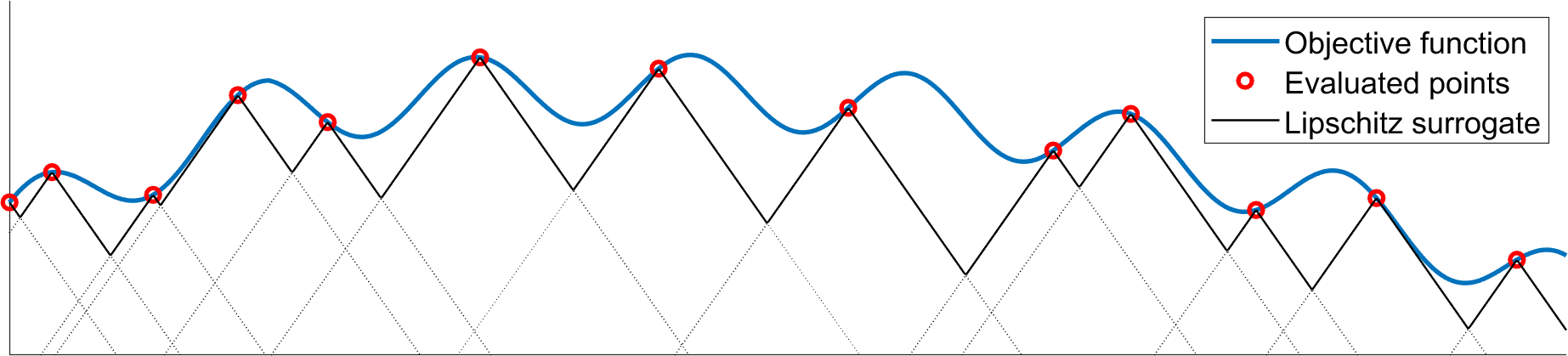
Figure 1: Visual representation of the Lipschitz-based surrogate in 1D.

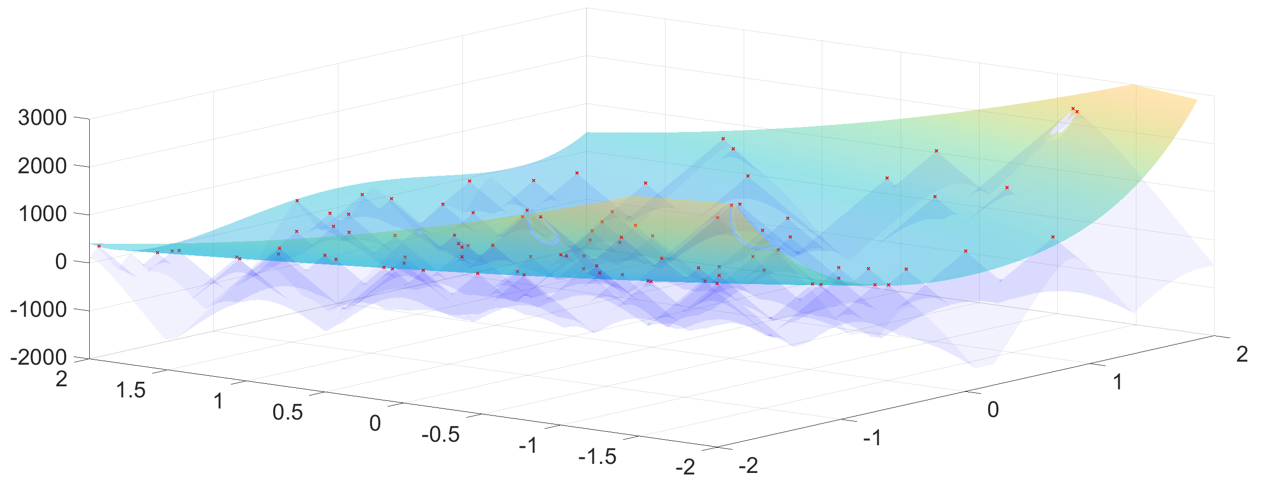
Figure 2: Visual representation of the Lipschitz-based surrogate on the Rosenbrock function in 2D. Sampled points are highlighted in red and the Lipschitz-based surrogate in light blue.

2.3 Differential Evolution

EAs are powerful methods for solving complex engineering optimization problems, that are difficult to approach with standard optimization methods. In this work, DE is employed as the optimization solver due to its straightforward structure and its global optimization capabilities. Several variants of DE have been developed to improve its performance Das11 . In general, there are four stages of DE: initialization, mutation, crossover, and selection. We assume we have a population at the current generation, $x=[x_{1},\dots,x_{t}]$, where each individual has dimension $D$, $x_{i}=(x^{1}_{i},\dots,x^{D}_{i})$. In this work, we utilize the DE/best/1 strategy for the mutation process of DE which, can be expressed as

$$v_{i}=x_{b}+F\cdot(x_{i_{1}}-x_{i_{2}}),$$ (4)

where $x_{b}$ is the current best solution, $x_{i_{1}}$ and $x_{i_{2}}$ are different randomly selected individuals from the population, and $F$ is a scalar number typically within the interval [0.4, 1] Das11 . The crossover stage of DE is conducted after mutation and has the following form:

$$u_{i}^{j}=\begin{cases}v_{i}^{j},\quad\textnormal{if }(U_{j}(0,1)\leq C_{r}\,|\,j=j_{rand}),\\ x_{i}^{j},\quad\textnormal{otherwise,}\end{cases}$$ (5)

where $u_{i}^{j}$ the $j$th component of $i$th offspring, $x_{j}^{i}$ and $v_{j}^{i}$ are the $j$th component of $i$th parent individual and the mutated individual, respectively. The crossover constant $C_{r}$ is between 0 and 1, $U_{j}(0,1)$ indicates a uniformly distributed random number, and $j_{rand}\in[1,\dots,D]$ is a randomly chosen index that ensures $u_{i}$ has at least one component of $v_{i}$. The interested reader can find more information about the intricacies of DE in Das11 .

3 Proposed LSADE Method

The proposed LSADE method has four distinct parts: 1) the DE-based generation of prospective points, 2) the global RBF evaluation of the prospective points, 3) the Lipschitz surrogate evaluation of the prospective points, and 4) the local optimization within a close range of the best solution found so far. The execution of parts 2) – 4) of the algorithm can be controlled based on chosen conditions, i.e., we may sometimes skip RBF surrogate evaluation, Lipschitz surrogate evaluation, or local optimization, if deemed advantageous.

At the beginning of the process, Latin hypercube sampling Forrester09 is used to generate the initial population of $t$ individuals, whose objective function is evaluated HTS . The best individual is found, a parent population of size $p$ is randomly selected from the evaluated points and a new population is constructed based on the DE rules (4) and (5). If the RBF evaluation condition is true, the new population is evaluated based on the RBF surrogate model. Then the best individual based on the RBF model has its objective function evaluated and is added to the whole population. This step constitutes a global search strategy.

Algorithm 1 Pseudocode of the LSADE.

1:Generate an initial population of $t$ points $X_{1},\dots,X_{t}$ and evaluate their objective function values. Denode the best solution as $X_{b}$.

2:Set $iter=0$ (iteration counter), $NFE$ = $t$ (number of function evaluations).

3:Use the evaluated points so far to estimate $k$ by (3) and to construct the RBF surrogate.

4:Sample $p$ points from the population as parents for DE.

5:Based on the DE rules (4) and (5), generate children.

6:Increase $iter$ by 1.

7:if RBF condition then

8:     Evaluate the children on the RBF surrogate.

9:     Find the child with the minimum RFB surrogate value, and add it to the population and evaluate its objective function value. Increase $NFE$ by 1.

10:if Lipschitz condition then

11:     Evaluate the children on the Lipschitz surrogate (1).

12:     Find the child with the minimum Lipschitz surrogate value, and add it to the population and evaluate its objective function value. Increase $NFE$ by 1.

13:if Local Optimization condition then

14:     Construct a RBF local surrogate model using the best $c$ solutions found so far.

15:     Find the bounds in each dimension for the local optimization (6).

16:     Minimize the local RBF surrogate model within the bounds. Denote the minimum as $\hat{X}_{m}$ and, if it is not already in the population, add it to the population and evaluate its objective function value. Increase $NFE$ by 1.

17:Find the best solution so far and denote it as $X_{b}$.

18:if $NFE<NFE_{max}$ then

19:     goto 3.

20:else

21:     terminate.

If the Lipschitz evaluation condition is true, the Lipschitz constant $k$ is estimated based on (3) and the new population is evaluated on the Lipschitz surrogate model (1). The best individual based on the Lipschitz surrogate model has its objective function evaluated and is added to the whole population.

If the Local optimization condition is true, we construct a local RBF surrogate model using the best $c$ solutions found so far, which we denote by $\hat{X}_{1},\dots,\hat{X}_{c}$. Additionally, we find the bounds for the local optimization procedure within those $c$ points:

$$\begin{split}lb(i)=\min_{j=1,\dots,c}{\hat{X}_{j}(i)},\quad i=1,\dots,D,\\ ub(i)=\max_{j=1,\dots,c}{\hat{X}_{j}(i)},\quad i=1,\dots,D,\end{split}$$ (6)

and perform a local optimization of the local RBF model within the bounds $[lb,ub]$. For local optimization we adapt a sequential quadratic programming strategy, which was also used by the winner of the 2020 CEC Single Objective Bound Constrained Competition IMODE20 . We find the local optimum and check, if it is not already in the population, before evaluating it and adding it to the population.

The evaluation of points based on the Lipschitz-based surrogate model can be thought of as an exploration step in the algorithm (and should increase our ability to find the regions of good solutions), whereas the evaluation of points based on the local optimization procedure can be thought of as an exploitation step of the algorithm (and should give us the means to improve the best solutions we have found so far).

The cycle of generating new population, evaluating it on the RBF and Lipschitz surrogate models and conducting the local optimization is carried out until a maximum number of objective function evaluations is reached. The pseudocode for the LSADE method is described in Algorithm 1.

4 Results and Discussion

To examine the effectiveness of the proposed method, we compare it with six other state-of-the-art algorithms on a testbed of standard benchmark functions Suga05 that are summarized in Table 1. Although there are more recent benchmark sets, such as ZZ2 , these were not yet used for benchmarking SAEAs. The dimensions for the comparison are $D=30,50,100,200$ for all of the benchmark functions. We also investigate the advantages of the individual components of the LSADE method, the choice of the conditions for using the different components, and the choice of basis functions for the RBF surrogates. The algorithm is implemented in MATLAB R2020b and runs on an Intel(R) Core(TM) i5-4460 CPU @ 3.20 GHz desktop PC.

Table 1: Benchmark functions used for the comparison

Problem	Description	Property	Optimum
F1	Ellipsoid	Unimodal	0
F2	Rosenbrock	Multimodal with narrow valley	0
F3	Ackley	Multimodal	0
F4	Griewank	Multimodal	0
F5	F10 in Suga05	Very complicated multimodal	-330
F6	F16 in Suga05	Very complicated multimodal	120
F7	F19 in Suga05	Very complicated multimodal	10

Table 2: Comparison of the individual components of LSADE on $D=[30,50]$.

$D$	F	R0$\,|\,$Li0$\,|\,$Lo0	R0$\,|\,$Li0$\,|\,$Lo1	R0$\,|\,$Li1$\,|\,$Lo0	R0$\,|\,$Li1$\,|\,$Lo1	R1$\,|\,$Li0$\,|\,$Lo0	R1$\,|\,$Li0$\,|\,$Lo1	R1$\,|\,$Li1$\,|\,$Lo0	R1$\,|\,$Li1$\,|\,$Lo1
	F1	1898	124.3	222.1	7.787	3.660	0.0041	7.237	0.010
	F2	4641	193.2	379.9	60.79	38.55	30.32	46.32	29.79
	F3	20.35	16.94	13.55	12.96	12.63	16.99	5.399	13.37
	F4	467.0	109.1	53.63	9.595	1.234	10.69	2.030	0.431
	F5	434.7	-126.9	33.95	-114.6	-133.2	-153.7	-133.4	-216.9
	F6	1154	814.7	587.6	488.4	608.8	603.3	490.8	440.7
30	F7	1348	1194	987.9	959.2	1062	1086	976.7	973.0
	F1	6365	148.5	1131	6.645	285.5	3.727	69.96	2.352
	F2	10279	283.5	1070	79.83	214.4	65.41	161.8	65.12
	F3	20.59	17.45	15.48	13.38	18.36	17.98	10.58	15.56
	F4	926.6	307.0	162.5	21.87	79.97	191.9	9.117	6.463
	F5	1185	30.64	396.1	-122.9	272.9	20.02	161.9	-138.0
	F6	1276	880.6	679.3	368.9	787.4	752.7	567.8	410.4
50	F7	1460	1296	1086	1019	1229	1238	1047	1077

4.1 Experiment Setting

For constructing both the local and the global RBF surrogate models we used the SURROGATES toolbox Viana11 with default settings (multiquadric RBF with parameter $c=1$). The DE coefficients were set to $F=0.5$ and $C_{r}=0.5$ kaz . The number of initial points were set to 100 for $D=[30,50]$ and 200 for $D=[100,200]$. The number of children was set to $D$. The local optimization uses the best $c=3\cdot D$ points found so far (or less if there are not enough points yet evaluated), and utilizes the sequential quadratic programming algorithm implemented in the FMINCON function with default parameters. The Lipschitz approximation parameter was set to $\alpha=0.01$. The maximum number of function evaluations was set to 1000 for all problems. For all benchmark functions, 20 independent runs are conducted to get statistical results. Finally, some of the more in-depth results regarding the sensitivity of the parameters of the LSADE algorithm are studied in the Appendix.

4.2 Comparison of Individual Components

Firstly, we assess the effectiveness of the individual components of the LSADE: the RBF surrogate, the Lipschitz surrogate, the local optimization procedure, and their combinations. This corresponds to setting the RBF condition, Lipschitz condition, and Local Optimization condition to true or false (1 or 0) for every iteration of the algorithm. We denote the 8 possible variations as a triplet (R – RBF, Li – Lipschitz, Lo – Local Optimization) R#$\,|\,$Li#$\,|\,$Lo#, where the “#” indicates if the condition was true or false. The R0$\,|\,$Li0$\,|\,$Lo0 variation does not use any optimization (as there is no rule to add points for evaluation) and instead just evaluates 1000 randomly selected points, using the entire computational budget. The results (mean of the best-found objective function values over the 20 runs) for the different variations in dimensions $D=[30,50]$ are reported in Table 2. Not surprisingly, the R0$\,|\,$Li0$\,|\,$Lo0 variant comes out being substantially worse than the other ones and is the only one that has its cells in the table colored in grey. The remaining variations are color-coded in the following way: the variant with the best (lowest) mean objective function value for a given problem instance has the corresponding cell in the table colored in a dark shade of green, the one with the worst (highest) mean objective function value has a dark red color, and the ones in between are ordered from green (better) to red (worse). This paradigm is also used in the subsequent tables for making straightforward comparisons. From Table 2 we can see that the “usefulness” of the individual components of LSADE is very problem-dependent, as there are instances, where adding either component may be beneficial or detrimental. However, based on the results, it seems advantageous to have the RFB condition be true, as the majority of the best results (11 of the 14 instances) were achieved by the R1 variants. As for the other two components, the situation is more nuanced – it is clear that they are both beneficial (the best results are always in a variant with either Li1 or Lo1), but the trade-off between adding one or the other needs to be be investigated in more detail.

Table 3: Comparison of the static rules for the Lipschitz and Local Optimization conditions, $D=[30,50].$

F1 [0.0036, 0.3671] Li$\,|\,$Lo 1 2 4 8 0 1 0.0102 0.0342 0.1328 0.3671 7.2373 2 0.0063 0.0085 0.0223 0.041 1.5932 4 0.0041 0.0048 0.0087 0.0129 0.6838 8 0.0047 0.0036 0.0062 0.0107 0.2917 0 0.0041 0.0046 0.0179 0.0063 3.6604	F2 [25.90, 32.59] Li$\,|\,$Lo 1 2 4 8 0 1 29.79 29.82 27.85 27.78 46.32 2 29.05 32.59 29.61 28.69 44.16 4 30.93 29.42 29.02 26.79 33.70 8 30.21 25.90 31.71 26.38 36.15 0 30.32 27.80 28.55 31.25 38.55	F3 [1.67, 15.78] Li$\,|\,$Lo 1 2 4 8 0 1 13.37 7.85 2.30 1.67 5.39 2 13.94 10.95 6.28 3.48 4.74 4 15.22 13.79 9.24 6.42 7.40 8 15.78 14.62 9.80 10.19 9.69 0 16.99 16.17 14.99 13.39 12.63
F4 [0.0035, 1.107] Li$\,|\,$Lo 1 2 4 8 0 1 0.431 0.290 0.508 0.595 2.030 2 0.586 0.144 0.109 0.197 1.253 4 0.702 0.120 0.075 0.078 1.082 8 1.107 0.160 0.035 0.061 1.025 0 10.69 2.193 0.615 0.139 1.234	F5 [-222.1, -168.5] Li$\,|\,$Lo 1 2 4 8 0 1 -216.9 -222.1 -212.1 -217.3 -133.4 2 -192.1 -206.8 -191.6 -168.5 -137.5 4 -189.3 -182.8 -185.3 -177.0 -140.4 8 -173.0 -178.5 -184.1 -177.0 -140.0 0 -153.7 -157.6 -167.8 -167.0 -133.2	F6 [418.7, 558.4] Li$\,|\,$Lo 1 2 4 8 0 1 440.7 423.8 438.0 437.4 490.8 2 476.1 440.5 462.8 418.7 493.7 4 492.1 466.4 471.9 463.9 511.6 8 558.4 529.0 509.1 495.0 543.8 0 603.3 592.8 597.7 587.1 608.9
F7 [958.1, 1036.4] Li$\,|\,$Lo 1 2 4 8 0 1 973.1 986.9 968.9 960.1 976.7 2 971.4 968.5 974.3 958.1 972.8 4 1010 998.7 994.3 981.9 1005 8 1036.4 1013 987.1 1014 1029 0 1086.8 1070 1040 1033 1062	Min and max mean values from the static rules for $D=50$ (disregarding rules with Li0 or Lo0)   F1   F2   F3   F4   F5   F6   F7 min 0.445 47.45 6.459 1.010 -138.0 363.2 1019 max 6.003 65.37 16.78 71.78 0.750 615.8 1195

Table 4: Comparison of the dynamic rules for the Lipschitz and Local Optimization conditions, $D=[30,50,100].$

$D$	F    [min,max]	1-4$\,|\,$8-1	1-6$\,|\,$8-1	1-8$\,|\,$8-1	1-4$\,|\,$6-1	1-6$\,|\,$6-1	1-8$\,|\,$6-1	1-4$\,|\,$4-1	1-6$\,|\,$4-1	1-8$\,|\,$4-1
	F1 [0.0061, 0.0113]	0.0113	0.0087	0.0069	0.0103	0.0107	0.0079	0.0082	0.0066	0.0061
	F2 [26.63, 27.06]	27.06	26.69	26.83	27.04	27.01	26.63	26.95	26.86	26.75
	F3 [1.122, 3.496]	1.308	1.152	1.480	1.235	1.279	1.122	2.546	3.496	3.327
	F4 [0.013, 0.051]	0.051	0.033	0.012	0.037	0.040	0.019	0.040	0.013	0.014
	F5 [-218.7, -196.3]	-218.7	-213.4	-214.5	-196.3	-197.0	-198.5	-213.1	-211.3	-215.5
	F6 [402.8, 439.6]	433.7	439.6	436.5	402.8	406.3	412.2	425.1	434.6	434.6
30	F7 [964.8, 978.9]	965.7	967.5	975.0	964.8	969.0	970.6	978.9	978.3	974.8
	F1 [0.839, 1.686]	1.358	1.686	1.126	1.400	1.339	0.839	1.499	1.248	1.144
	F2 [47.65, 58.89]	47.65	47.73	49.71	50.12	50.25	51.67	58.15	58.69	57.93
	F3 [6.876, 12.42]	6.876	7.469	8.467	8.995	8.858	9.344	11.02	12.03	12.42
	F4 [0.749, 1.097]	0.819	0.789	0.749	0.887	0.898	0.879	1.031	1.045	1.097
	F5 [-136.4, -97.26]	-98.78	-97.26	-99.96	-108.7	-107.5	-123.9	-136.4	-132.3	-131.1
	F6 [367.2, 405.2]	370.3	379.2	405.2	384.8	375.1	388.8	367.2	384.1	380.7
50	F7 [1015, 1068]	1016	1027	1053	1015	1025	1033	1037	1051	1068
	F1 [88.13, 125.3]	112.8	105.2	94.59	97.99	106.3	88.13	125.3	110.3	112.0
	F2 [123.6, 147.5]	140.6	135.7	132.8	138.0	141.1	123.6	147.5	129.0	138.4
	F3 [12.05, 15.11]	12.05	12.77	13.41	13.25	13.48	14.06	14.78	14.90	15.11
	F4 [6.517, 18.74]	6.517	7.434	12.47	7.574	8.522	11.37	10.64	14.74	18.74
	F5 [34.52, 117.6]	60.28	117.6	82.19	92.60	96.94	94.94	34.52	44.79	82.18
	F6 [332.7, 363.0]	332.7	343.6	360.0	343.4	345.0	354.1	333.7	351.5	363.0
100	F7 [1144, 1193]	1144	1162	1185	1162	1176	1193	1160	1184	1192

4.3 Tuning the Lipschitz and Local Optimization Conditions

As LSADE allows controlling the addition of points for evaluation for the individual surrogates, we use it for tuning the balance between the exploration via the Lipschitz condition and the exploitation via the Local Optimization condition (from this point onward, the RBF condition is always true). We start by using static rules for both conditions to be true, which will be based on the current iteration number. We consider 5 possibilities: 1 – iteration number divisible by 1 (i.e., every iteration); 2 – iteration number divisible by 2 (every other iteration); 4 – iteration number divisible by 4; 8 – iteration number divisible by 8; 0 – never. For example, Li2$\,|\,$Lo0 means that points for real function evaluation based on the Lipschitz condition are added every two iterations and the Local Optimization is not used at all. In this setting, there were 25 variations in total. The results of the computations (mean over the 20 independent runs) for all 25 variations of the considered static rules for $D=30$ are reported in Table 3. In the table, next to the benchmark function identifier is the best and worst results in square brackets, where we chose to omit the rules with Li0 or Lo0 (as these were often quite a lot worse than the other ones). Also in Table 3 are the aggregate results for $D=50$, while the detailed results can be found in the Appendix. These results suggest that using both the Lipschitz surrogate and the local optimization procedure is beneficial for every benchmark problem. The Lispchitz surrogate is especially well suited for problems F3 and F5-F7 (which are the ones with the complicated multimodal structure). However, none of the variations performed very well for all the considered problems, and the difference between the best and the worst variation for a given problem (even with disregarding rules with Li0 or Lo0) was quite high.

Since the Lipschitz surrogate should serve as an exploration-enhancing part of the algorithm, it is only natural that the frequency of its use should diminish as the iterations progress, to make space for the parts of the algorithm that focus on the exploitation of prospective areas. Hence, we devised several dynamic rules that decrease the frequency of using the Lipschitz surrogate, and increase the frequency of the local optimization, both in a linear manner. For instance, the variant Li1-4$\,|\,$Lo8-1 starts with the Lipschitz surrogate being used every iteration and the local optimization procedure being used every 8 iterations, and ends with the Lipschitz surrogate being used every 4 iterations and the location optimization procedure being used every iteration. The individual conditions for the 9 considered variations can be found in the Appendix. The results of the computations with the dynamic rules for $D=[30,50,100]$ are summarized in Table 4. When comparing the results from the dynamic and the static rules, two important observations can be made. First, the dynamic rules have a much smaller interval between the best and the worst variation for the given problem instance, while the values of the best instances remain comparable. Second, there is one variation that stands out as having good results across many problem instances, particularly in higher dimensions.

The Li1-4$\,|\,$Lo8-1 variant of the algorithm was selected as the best-performing one and will be used as the default variation for the subsequent modifications. It would probably be advantageous to devise a scheme that automatically decides on the frequency of using the Lipschitz surrogate or the local optimization procedure based on the past improvements and to tailor it for each problem separately. This is a research topic we plan to investigate in the future.

4.4 Comparison of Different RBFs

Next, we investigate the effect of using different basis functions for the two RBF surrogate models (one global and one local). We use the Li1-4$\,|\,$Lo8-1 rule for the Lipschitz and Local Optimization conditions that was tuned for the multiquadratic (MQ) basis function and run the algorithm with cubic, thin plate spline (TPS), linear, and Gaussian basis function for the two RBFs instead. The results of the computations can be found in Table 5. From these results, it is apparent that the choice of the basis function has a substantial effect on the performance of the algorithm. Both the multiquadratic and the cubic basis functions performed very well on most of the problem instances, the TPS function was consistently mediocre, the Gaussian function performer mostly poorly (apart from the F1 problem) and the linear function performed the worst. The convergence histories of these variations can be found in the Appendix. Once again, it would very likely be beneficial to devise a scheme that would automatically choose the “appropriate” basis function for each problem separately. In the same vein, using different RBFs for the local and global models could also improve the performance of the algorithm.

Table 5: Comparison of different basis functions, $D=[30,50,100]$.

$D$	F	MQ	Cubic	TPS	Linear	Gaussian
	F1	0.011	0.011	0.509	6.276	0.003
	F2	27.06	27.77	31.86	93.31	28.10
	F3	1.308	0.256	0.418	4.946	4.164
	F4	0.051	0.176	0.577	1.883	0.944
	F5	-218.7	-172.6	-155.9	-143.6	-9.30
	F6	433.7	426.2	437.2	448.1	526.5
30	F7	965.7	938.8	944.4	965.8	951.7
	F1	1.358	0.434	7.556	54.78	0.191
	F2	47.65	47.98	62.20	221.8	47.71
	F3	6.876	0.695	1.822	10.56	5.161
	F4	0.819	0.380	0.801	5.668	0.930
	F5	-98.78	-10.03	2.45	82.64	274.9
	F6	370.3	481.6	464.5	521.6	585.6
50	F7	1016	976.3	979.6	1054	985.7
	F1	112.8	30.94	279.5	766.6	20.39
	F2	140.6	106.4	331.7	714.5	165.1
	F3	12.05	4.622	9.089	16.65	8.965
	F4	6.517	0.816	2.190	69.61	0.946
	F5	60.28	646.8	527.1	701.2	1012
	F6	332.7	550.4	522.9	572.5	596.3
100	F7	1144	1056	1146	1248	1112

Table 6: Comparison with other algorithms, average objective function value.

$D$	F	SAMSO	MGP-SLPSO	GSGA	SAGWO	ESAO	SA-COSO	LSADE-MQ	LSADE-C
	F1	0.0053	0	0.073	0.00007	0.027	3.85	0.0113	0.0115
	F2	28.3	100	27.60	28.30	25.04	59.9	27.06	27.77
	F3	0.628	6.58	0.023	0	2.521	5.01	1.308	0.256
	F4	0.538	0.013	0.228	0.015	0.953	1.44	0.051	0.176
	F5	-239	-220	-203.0	-128.8	6.325	-57.4	-218.7	-172.6
	F6	372	N/A	424.7	489.8	N/A	528	433.7	426.2
30	F7	922	952	927.2	973.2	931.6	969	965.7	938.8
	F1	0.513	0	0.621	0.004	0.740	46.6	1.358	0.434
	F2	50.1	120	48.21	49.06	47.39	253	47.65	47.98
	F3	1.53	9.31	0.022	0	1.431	8.86	6.876	0.695
	F4	0.666	0.154	0.346	0.025	0.94	5.63	0.819	0.380
	F5	-169	33	-75.82	98.39	198.6	235	-98.78	-10.03
	F6	326	N/A	403.3	502.0	N/A	613	370.3	481.6
50	F7	970	1060	970.7	1044.1	975.3	1080	1016	976.3
	F1	72.1	0.00005	12.33	0.139	1283	985	112.8	30.94
	F2	286	612	109.1	123.4	578.8	2500	140.6	106.4
	F3	6.12	14.3	1.31	0	10.36	15.9	12.05	4.622
	F4	1.06	0.715	0.706	0.023	57.34	63.5	6.517	0.816
	F5	737	885	672.5	800.1	713.4	1420	60.28	646.8
	F6	513	N/A	447.2	518.6	N/A	807	332.7	550.4
100	F7	1290	1390	1256	1350	1372	1410	1144	1056
	F1	1520	N/A	N/A	N/A	17616	16382	3959	793.6
	F2	1150	N/A	N/A	N/A	4318	16411	927.2	576.3
	F3	12	N/A	N/A	N/A	14.69	17.86	15.20	14.58
	F4	9.03	N/A	N/A	N/A	572.9	577.7	135.6	2.892
	F5	4960	N/A	N/A	N/A	5389	3927	1416	2305
	F6	684	N/A	N/A	N/A	N/A	N/A	578.7	722.7
200	F7	1340	N/A	N/A	N/A	1456	1347	1276	1222

4.5 Comparison with Other Algorithms

The proposed LSADE method is compared with six SAEAs, namely, SA-COSO SACOSO17 , ESAO ESAO19 , SAGWO Dong20 , GSGA Cai20 , MGP-SLPSO Tian19 , and SAMSO Li21 , which are all methods for high-dimensional expensive problems that can be compared on the same testbed (although some of the problems have not been evaluated by some of the algorithms). SA-COSO is a surrogate-assisted cooperative swarm optimization algorithm, in which a surrogate-assisted particle swarm optimization algorithm and a surrogate-assisted social learning based particle swarm optimization algorithm cooperatively search for the global optimum. ESAO is an evolutionary sampling-assisted optimization method that combines global and local search to balance exploration and exploitation, and employs DE as the optimization method. SAGWO utilizes the grey wolf optimization algorithm and conducts the search in three phases, initial exploration, RBF-assisted meta-heuristic exploration, and knowledge mining on RBF. GSGA uses a surrogate-based trust region local search method, a surrogate-guided GA updating mechanism with a neighbor region partition strategy, and a prescreening strategy based on the expected improvement infilling criterion of a simplified Kriging in the optimization process. MGP-SLPSO employs a multi-objective infill criterion that considers the approximated fitness and the approximation uncertainty as two objectives for a Gaussian process assisted social learning particle swarm optimization algorithm. SAMSO is a a surrogate-assisted multiswarm optimization algorithm for high-dimensional problems, which includes two swarms: the first one uses the learner phase of teaching-learning-based optimization to enhance exploration and the second one uses the particle swarm optimization for faster convergence. The data for the comparison were obtained from the corresponding papers, with the exception of the data for SA-COSO and ESAO, which were obtained from Li21 .

The average objective function value for the considered algorithms and for the LSADE algorithm with multiquadratic and cubic RBFs are reported in Table 6. More detailed results, including the best results, worst results, and standard deviations of the independent runs for all the considered algorithms can be found in the Appendix. Looking at $D=30$ first, we can see that there is no one algorithm that is strictly better than all the others on all the benchmark functions. The less complicated functions F1-F4 are dominated by MGP-SLPSO, GSGA, SAGWO, and EASO, while for the more complicated functions F5-F7 SAMSO seems to be the best. Both of the LSADE variants come out somewhere in the middle for all problems. In a direct comparison with LSADE, the best ones are SAMSO (better in 5/7 than LSADE-MQ) and GSGA (better in 5/7 than LSADE-C). For $D=50$ the situation is quite similar: the best algorithms for the less complicated problems are MGP-SLPSO, SAGWO, and ESAO, while SAMSO dominates the more complicated problems again. Both of the LSADE variants are, once again, somewhere in the middle. In a direct comparison with LSADE, the SAMSO is the best (better in 6/7 than LSADE-MQ). However, the situation changes substantially for higher dimensions. For $D=100$, MGP-SLPSO, LSADE-C, and SAGWO dominate the less complicated functions, while LSADE-MQ and LSADE-C have the best results for the more complicated function. In direct comparison with LSADE, the best ones are GSGA and SAGWO (both 4/7 for both variants). For $D=200$, only three of the six considered algorithms reported results (possibly because of prohibitively large computational times as will be investigated in the following section). In these largest instances, LSADE-MQ and LSADE-C were the best choices for all problems with the exception of F3 for which SAMSO was the best.

The convergence histories of the considered algorithms for $D=[50,100,200]$ are depicted in Figures 3 and 4, where on the $y$ axis are not the objective function values, but the difference between the objective function value and the corresponding optimum (otherwise, the $\log$ operator would fail for F5). For $D=200$, the convergence histories of the six compared algorithms were not available, and the convergence history of LSADE can be found in the Appendix. From these results, it is quite clear that the LSADE algorithm with properly tuned rules for using the newly proposed Lipschitz surrogate model and local optimization procedure compares well to the state-of-the-art SAEAs, especially for the high-dimensional highly complicated benchmark problems.

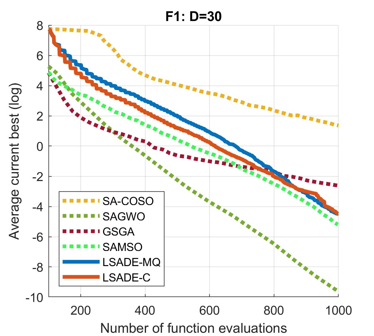
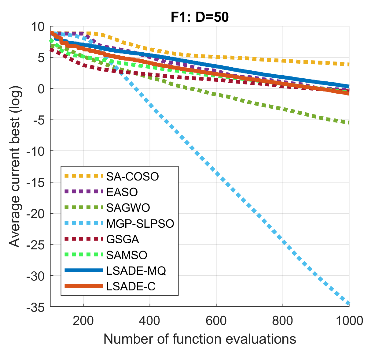
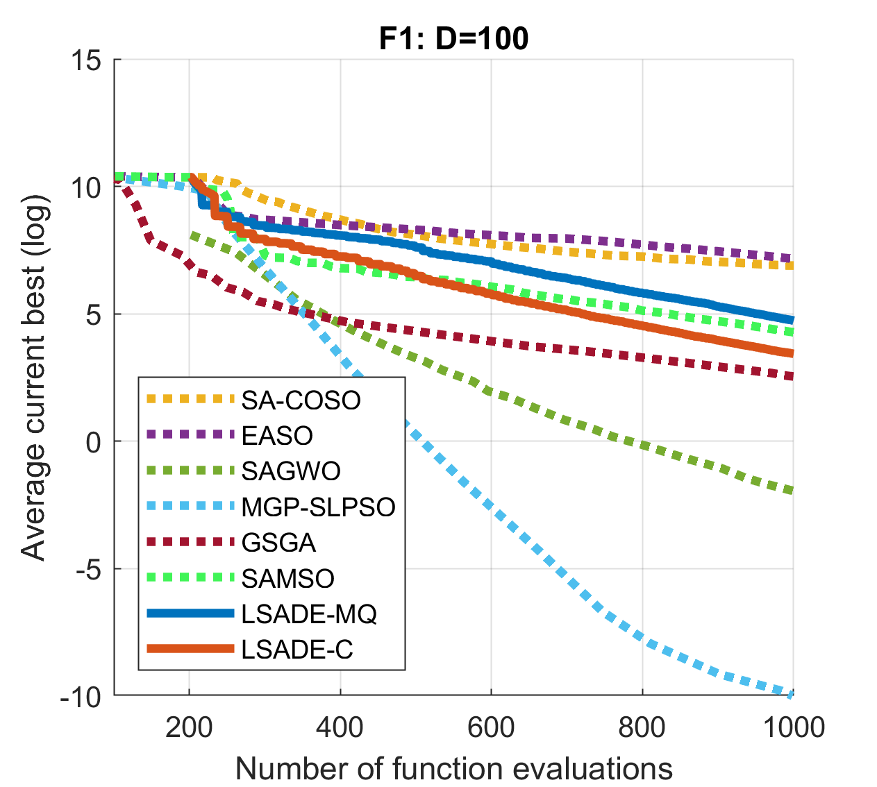
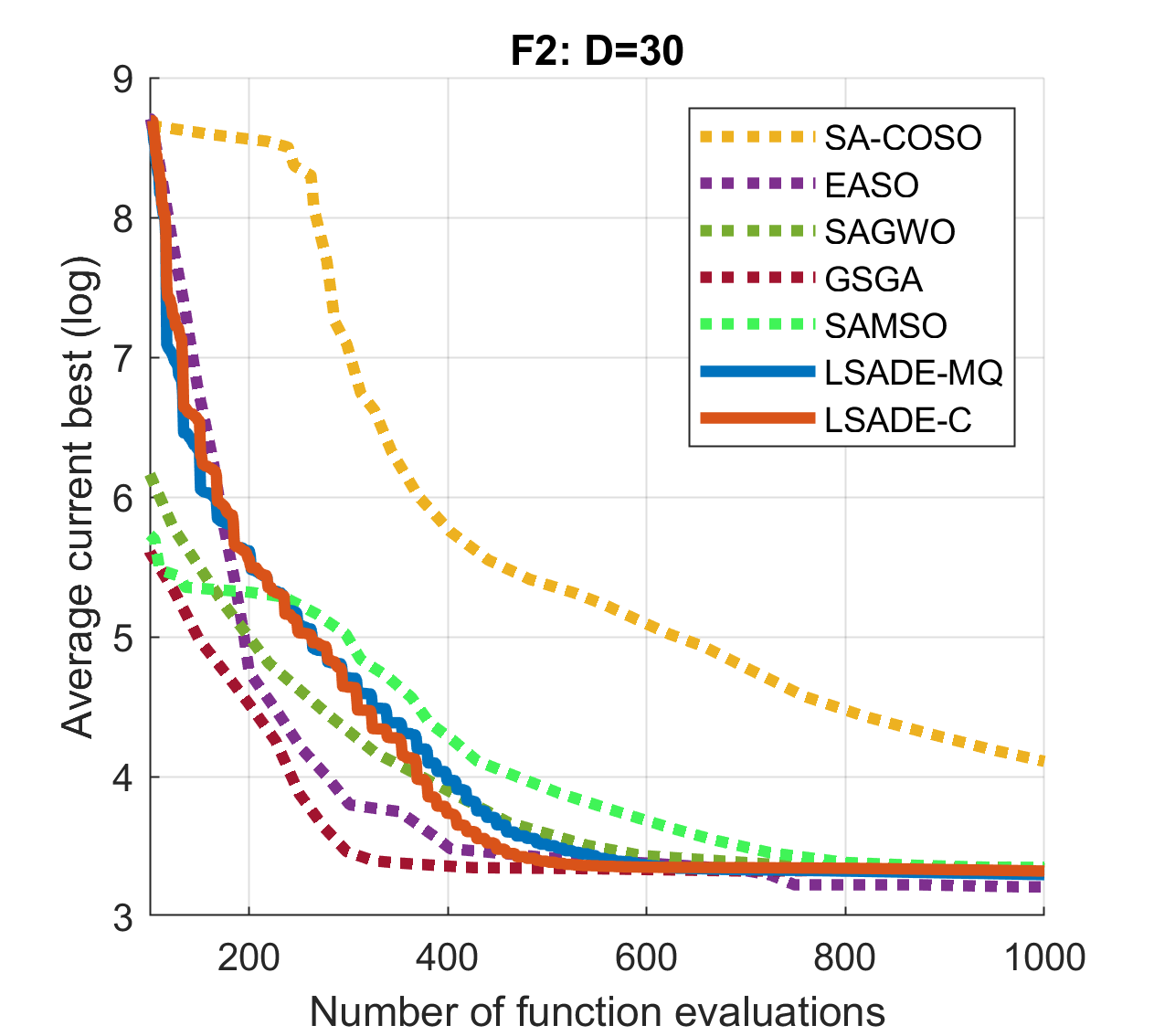
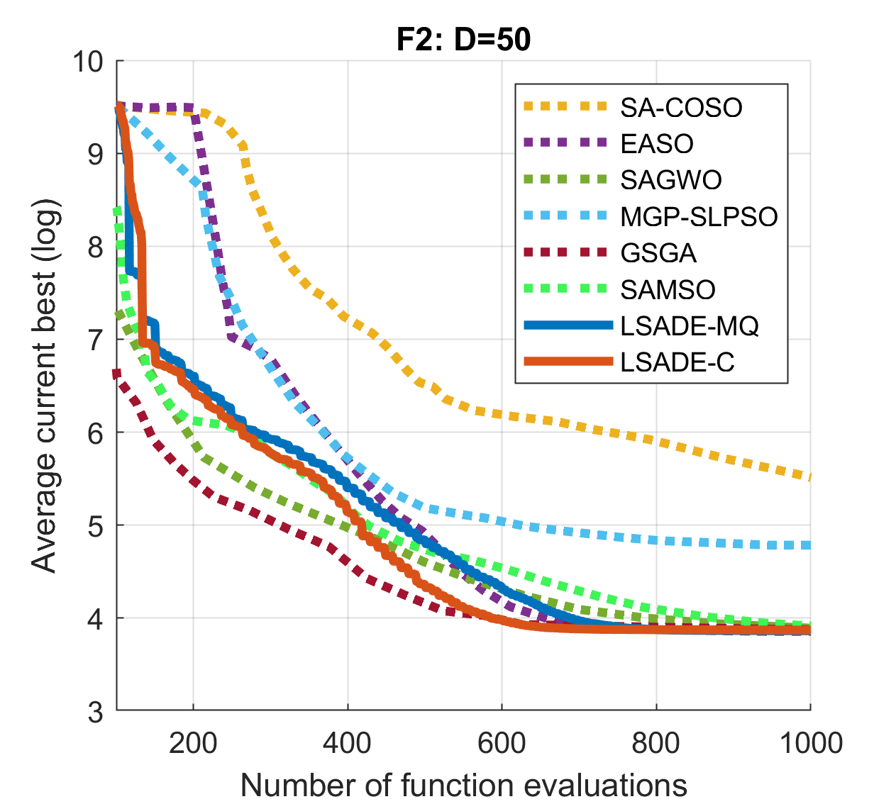
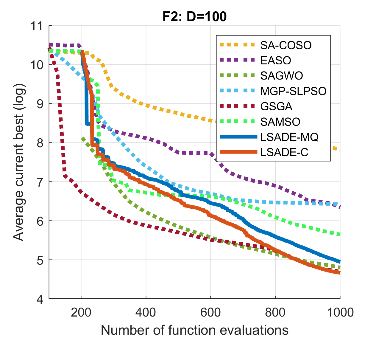
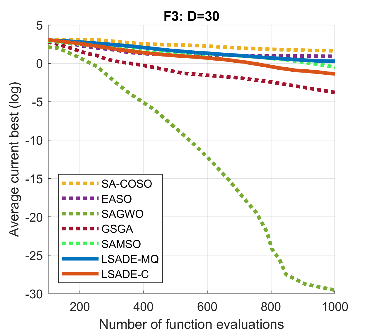
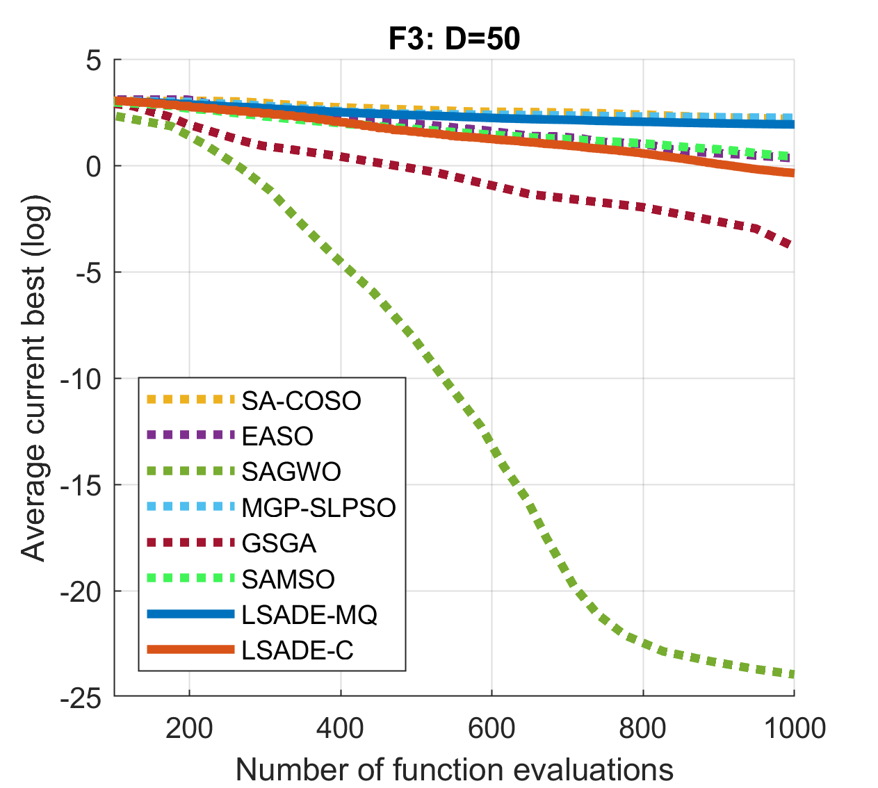
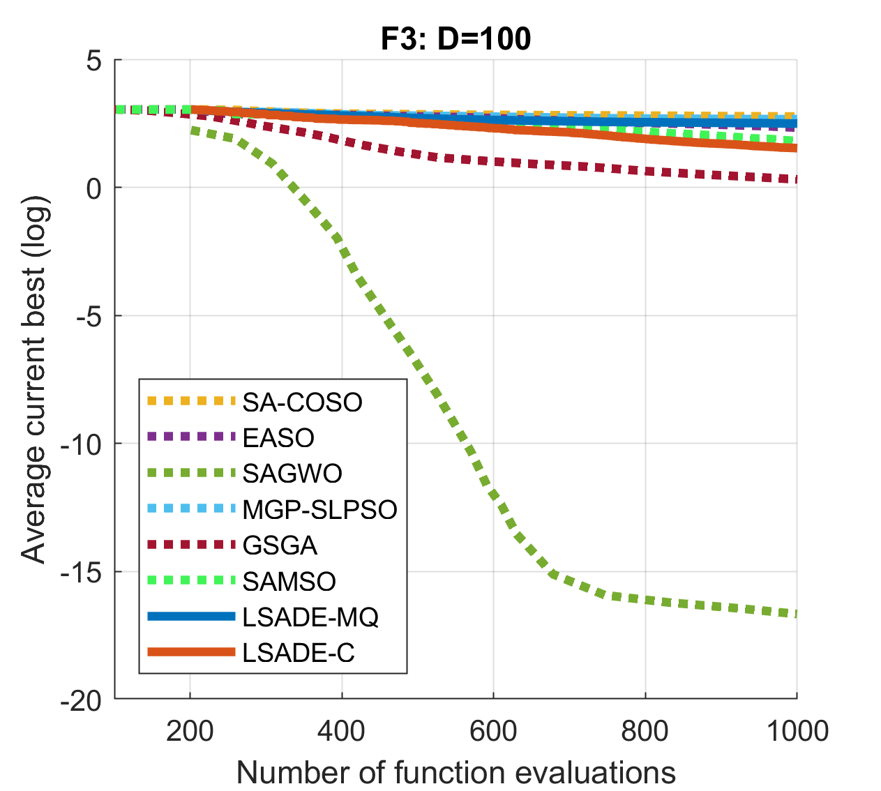
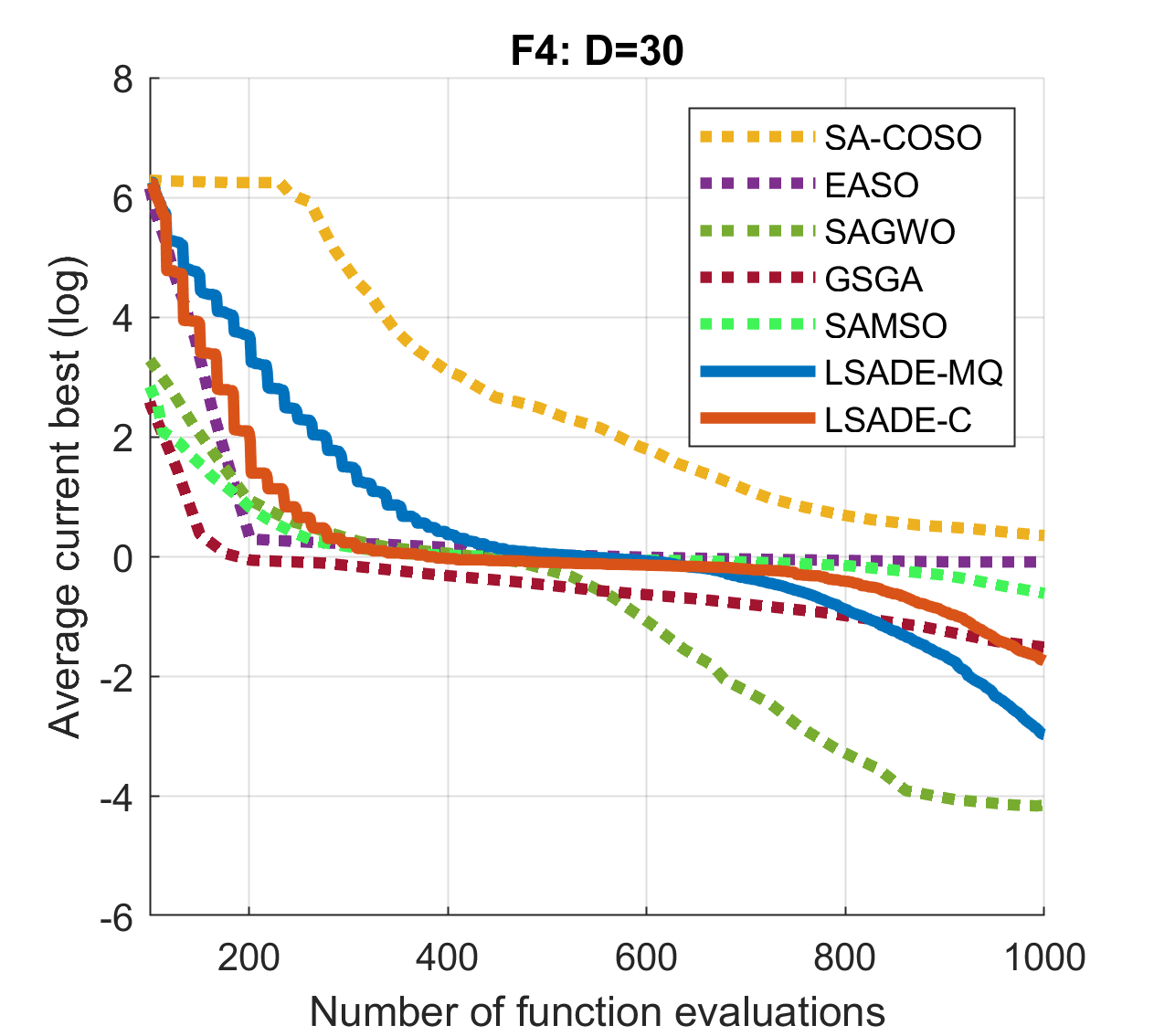
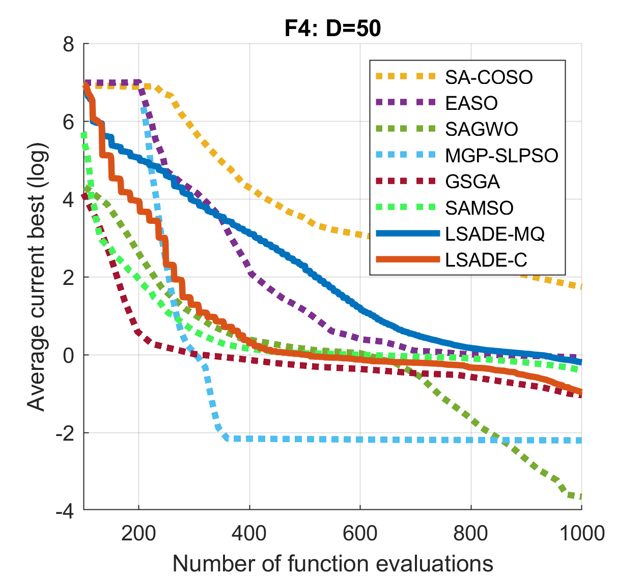
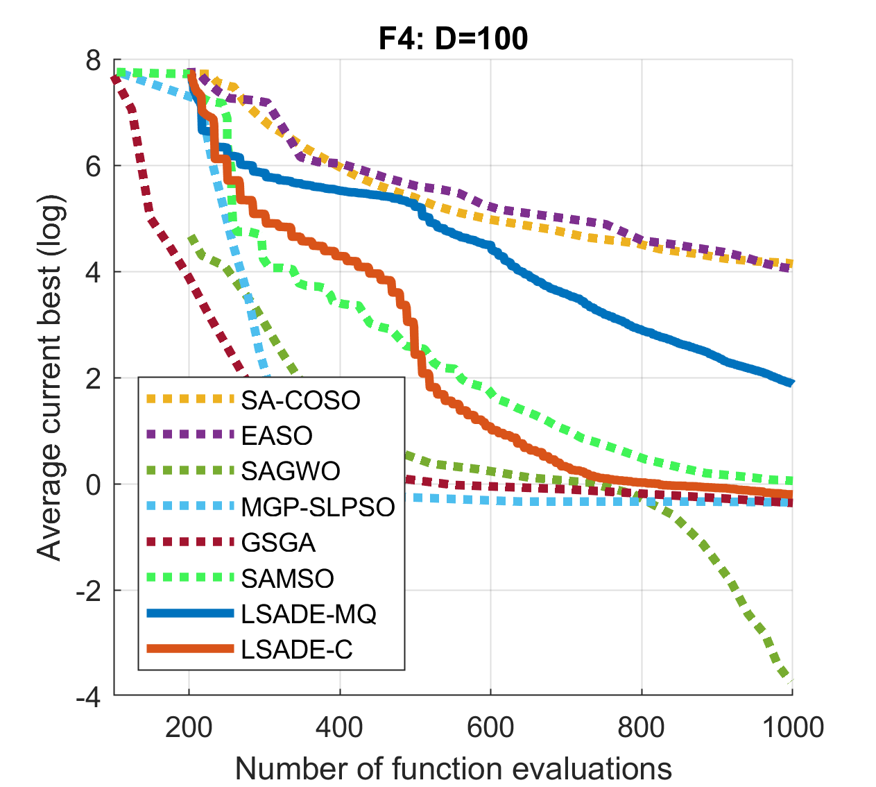
Figure 3: Convergence history of the considered algorithms on the benchmark functions F1–F4 in dimensions $D=[30,50,100]$.

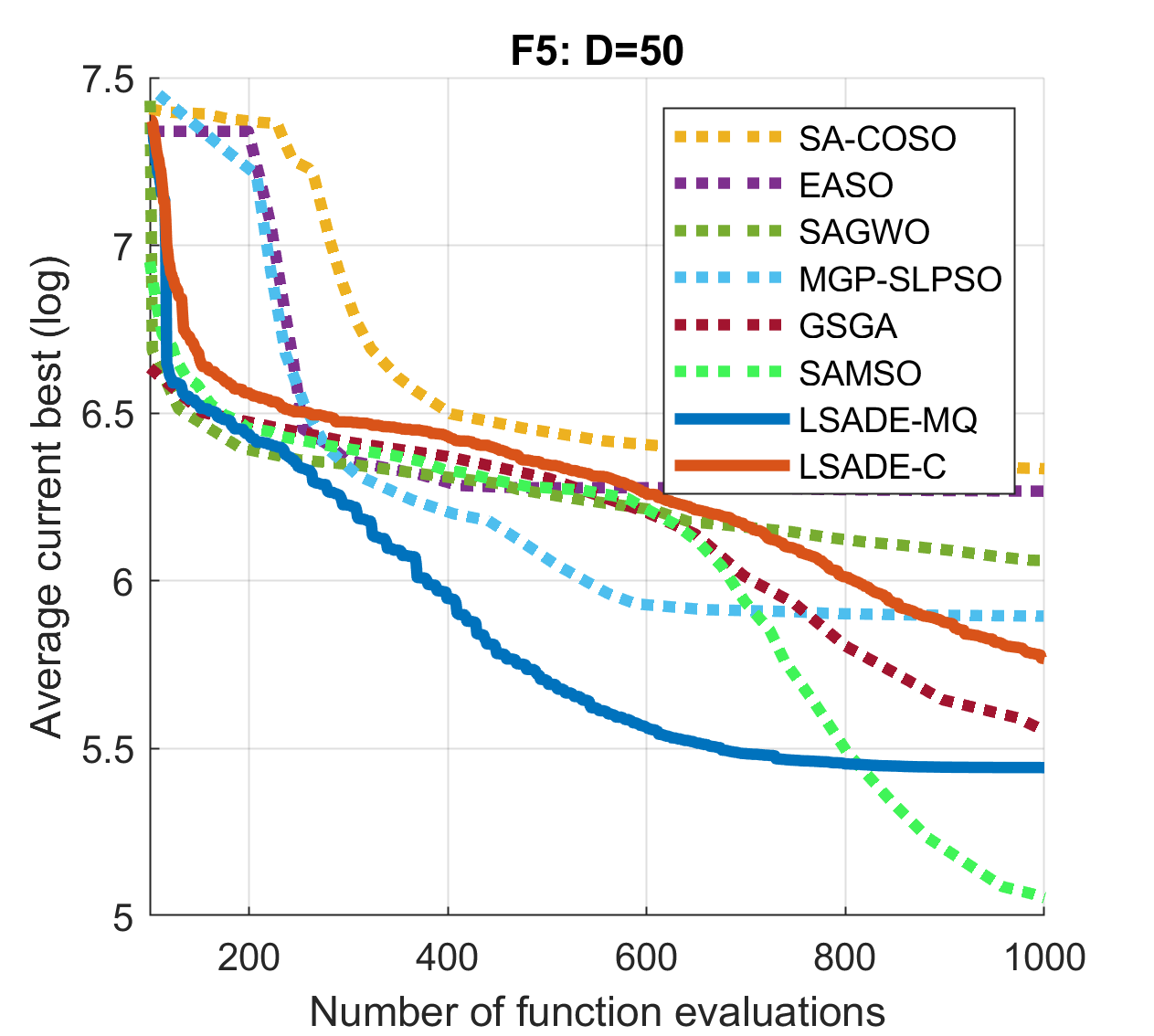
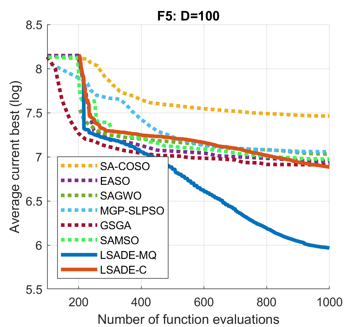
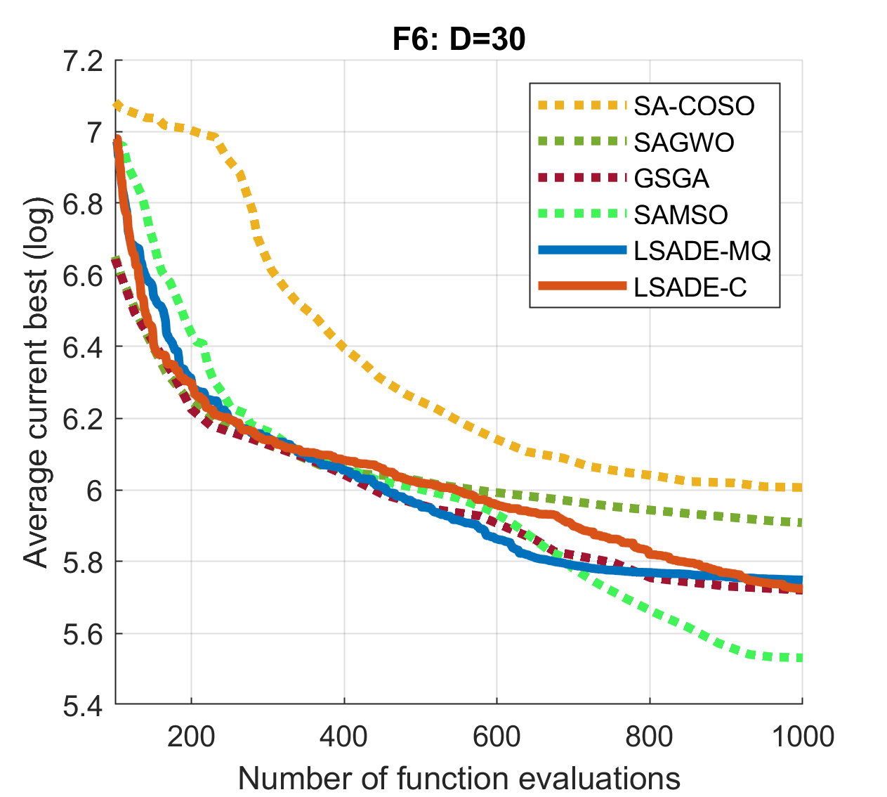
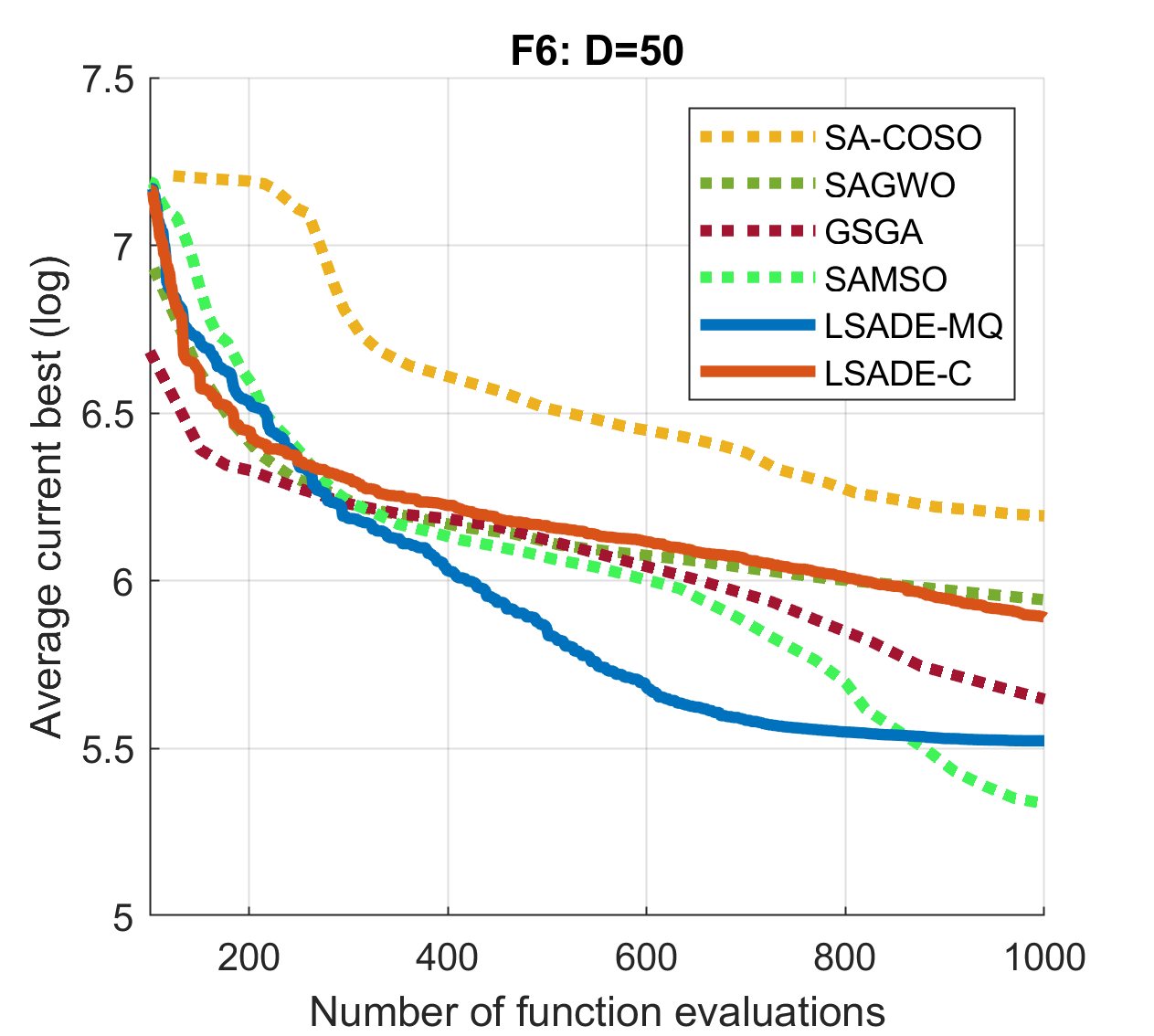
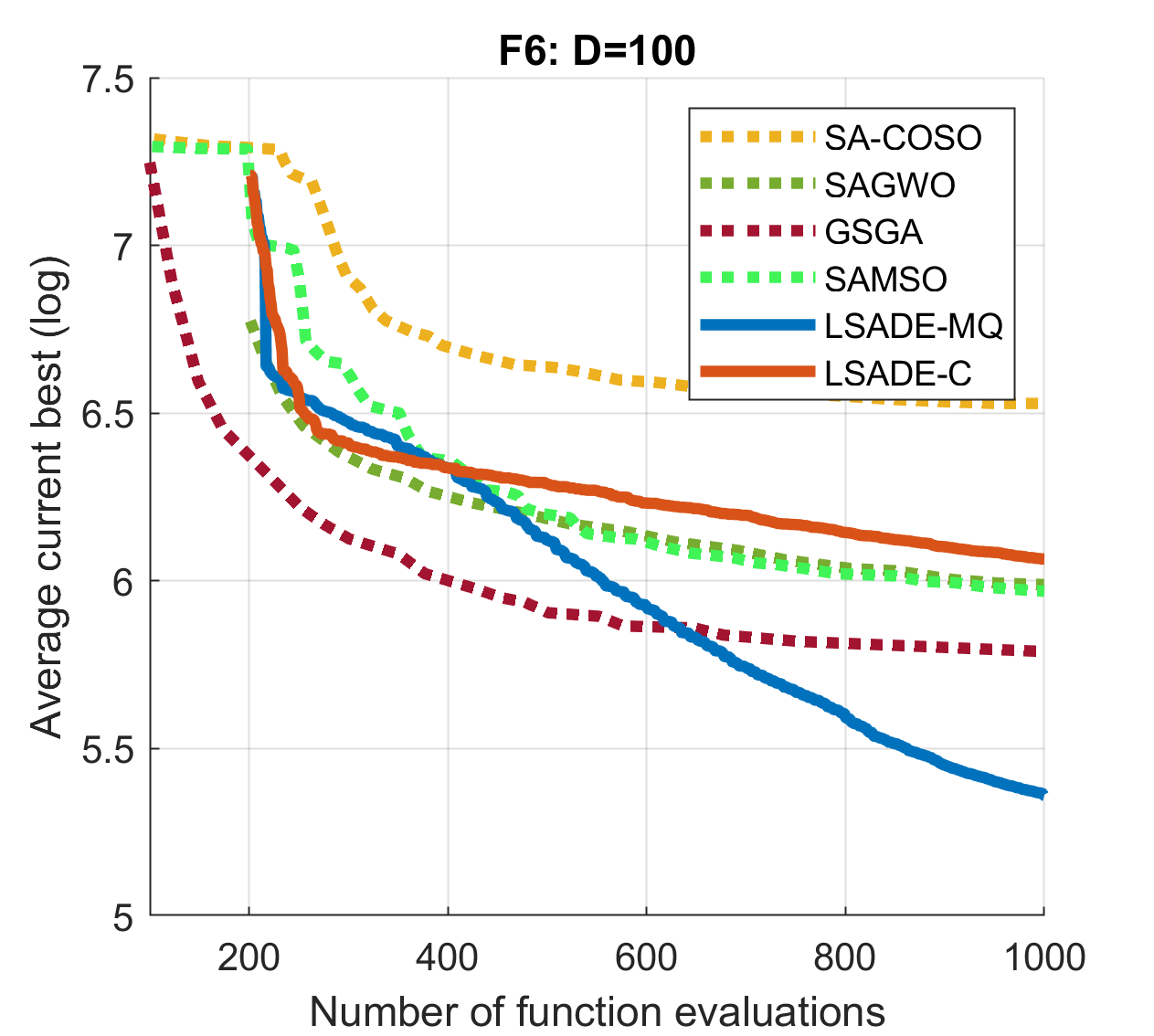
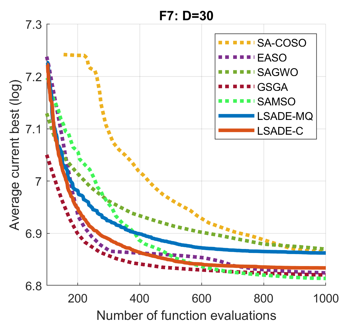
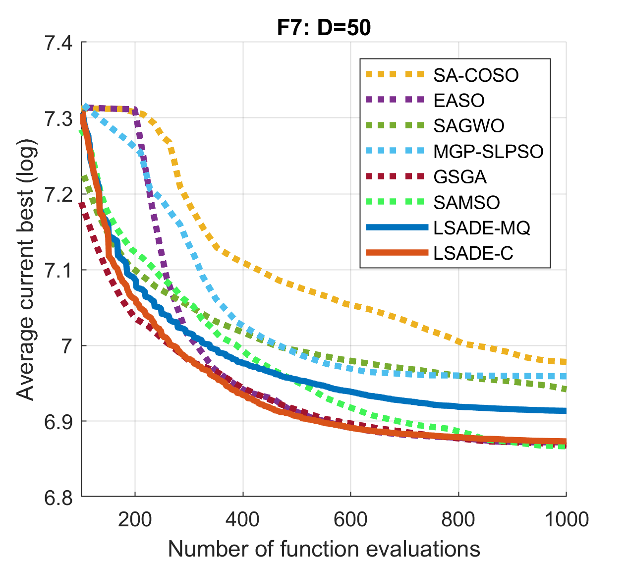
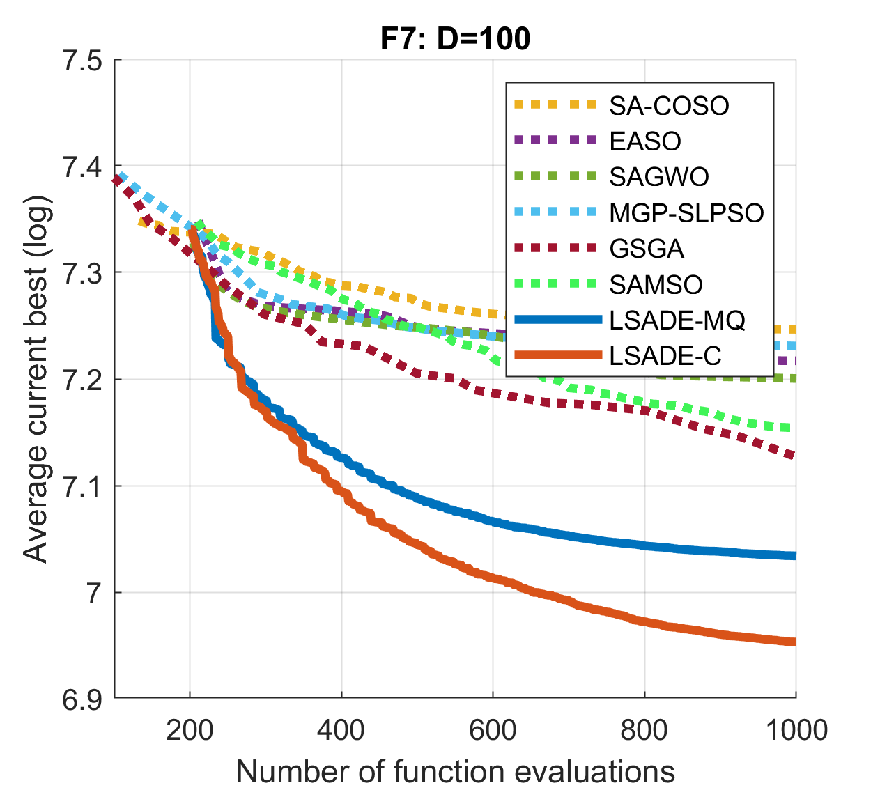
Figure 4: Convergence history of the considered algorithms on the complicated benchmark functions F5–F7 in dimensions $D=[30,50,100]$.

4.6 Computational Complexity

For LSADE the computational complexity mainly consists of five parts: the computation time for initial search, creating and evaluating the local and global RBF surrogate models, creating and evaluating the Lipschitz model, local optimization, and real function evaluations. In the following, we focus on empirical analysis of the computational time for the surrogates and the local optimization procedure, as the time for real function evaluations depends on the problem the algorithm is applied to solve (these evaluations are expected to be costly, otherwise the algorithm should not be used). First, we compare the computational times for the individual components of the LSADE algorithm, using the R0$\,|\,$Li0$\,|\,$Lo1, R0$\,|\,$Li1$\,|\,$Lo0, and R1$\,|\,$Li0$\,|\,$Lo0 variants of the algorithm for the computation of the benchmark problems for $D=[30,50]$. The results of these computations are reported in Table 7. We observe that the computation of Lipschitz surrogate model is significantly less computationally demanding than the computation of the (multiquadratic) RBF surrogate model. Unsurprisingly, the computational requirements for the local optimization are quite large, as these computations also contain the construction of the local RBF surrogate model.

Table 7: Computational time [s] of the individual components of LSADE, $D=[30,50]$.

$D$	F	R0$\,|\,$Li0$\,|\,$Lo1	R0$\,|\,$Li1$\,|\,$Lo0	R1$\,|\,$Li0$\,|\,$Lo0
30	F1	76.35	3.44	38.96
	F2	43.12	3.36	38.97
	F3	46.59	3.19	38.36
	F4	30.02	3.03	37.46
	F5	70.94	3.40	39.10
	F6	55.24	7.01	43.27
	F7	74.55	7.03	44.49
50	F1	239.17	5.46	51.15
	F2	158.25	5.57	51.57
	F3	153.27	5.41	53.34
	F4	85.77	5.78	53.40
	F5	231.53	5.75	52.91
	F6	170.06	9.62	56.26
	F7	229.90	9.43	55.92

Table 8: Comparison with other algorithms, computational times [s].

$D$	SA-COSO	MGP-SLPSO	SAGWO	LSADE-MQ	LSADE-C
30	N/A	N/A	226	33.24	54.14
50	595	666	428	59.8	83.45
100	833	741	1099	164.1	167.7
200	N/A	N/A	N/A	591.3	685.6

The computational requirements for different variants of the LSADE algorithm will differ based on the number of RBF and Lipschitz surrogate evaluations, and on the number of times the local optimization procedure is used. The number of times these individual components were used for the variant of LSADE that was chosen for numerical comparisons (Li1-4$\,|\,$Lo8-1), as well as for the other variants can be found in the Appendix. The average computational times of LSADE-MQ and LSADE-C for the benchmark problems for $D=[30,50,100,200]$ can be found in Table 8. The computational times for different variants of LSADE as well as for different basis functions can also be found in the Appendix. Also in Table 8 are the computational times of SA-COSO, MGP-SLPSO, and SAGWO that were reported in the respective papers. As for the other compared algorithms, GSGA reported a computational time of 3 hours for the function F3 in $D=100$, and EASO and SAMSO did not include an empirical analysis of computational complexity. This comparison gives a clue as to why were the MGP-SLPSO, SAGWO, and GSGA algorithms not used for solving the large $D=200$ problems – the computational times become a bit prohibitive for a large number of runs on numerous benchmark functions (but not necessarily prohibitive for a real application). On the other hand, the computational requirements for LSADE remain relatively low, with a dependence on the problem dimension that is roughly quadratic (at least for the considered benchmark problems). This is another indication that the LSADE algorithm is well suited for high-dimensional expensive problems.

The complexity of the Lipschitz surrogate itself depends on two main operations: on the estimation of the Lipschitz constant and on the evaluation of the surrogate. Through empirical analysis (performed on F7) shown in Table 9 we can see that for the Lipschitz constant estimation there is a linear dependence of the computational time on the problem dimension $D$ and a quadratic dependence on the number of evaluated points $n$. Similarly, in Table 10, we find that the computational time for evaluating the Lipschitz surrogate depends linearly on both $D$ and $n$.

Table 9: Dependence of computational time [s] of computing the Lipschitz constant estimate on dimension $D$ and on the number of points for surrogate construction $n$.

		$D$
		30	50	100	200	500	1000
$n$	30	2.13E-04	9.45E-05	1.34E-04	1.81E-04	2.76E-04	4.84E-04
	50	3.31E-04	3.03E-04	2.97E-04	4.52E-04	7.54E-04	1.32E-03
	100	9.77E-04	8.73E-04	1.11E-03	1.60E-03	2.96E-03	5.40E-03
	200	3.02E-03	3.41E-03	5.14E-03	6.27E-03	1.20E-02	2.13E-02
	500	1.87E-02	2.16E-02	2.73E-02	3.91E-02	7.56E-02	1.34E-01
	1000	6.98E-02	8.81E-02	1.13E-01	1.56E-01	3.11E-01	5.39E-01

Table 10: Dependence of computational time [s] for evaluating 10,000 points on the Lipschitz surrogate model on dimension $D$ and on the number of points for surrogate construction $n$.

		$D$
		30	50	100	200	500	1000
$n$	30	7.09E-02	6.81E-02	8.57E-02	1.19E-01	2.15E-01	3.92E-01
	50	8.97E-02	1.05E-01	1.32E-01	1.85E-01	3.43E-01	6.08E-01
	100	1.60E-01	1.88E-01	2.47E-01	3.53E-01	6.73E-01	1.19E+00
	200	3.07E-01	3.61E-01	4.81E-01	6.91E-01	1.33E+00	2.38E+00
	500	7.29E-01	8.88E-01	1.17E+00	1.69E+00	3.30E+00	5.93E+00
	1000	1.45E+00	1.76E+00	2.33E+00	3.37E+00	7.06E+00	1.22E+01

5 Conclusion

In this paper, we proposed a novel Lipschitz-based surrogate model for computationally expensive problems and used it to develop LSADE, a differential evolution-based surrogate-assisted evolutionary algorithm. The LSADE algorithm utilizes the combination of the Lipschitz-based and standard RBF surrogate models and a local optimization procedure to balance the exploration and the exploitation on a limited computational budget. The proposed LSADE algorithm was evaluated and its hyperparameters (such as the choice of the particular RBF surrogate and the frequency of its individual components) were tuned on a testbed of seven widely used 30, 50, 100, and 200 dimensional benchmark problems. The computational results show its effectiveness and competitiveness with other state-of-the-art algorithms, especially for complicated and high-dimensional problems.

There still remains much room for further improvements. The conditions for including new points based on the Lipschitz surrogate and local optimization could be made in an adaptive manner based on the progress of the algorithm. Similarly, the use of different RBFs or ensembles within the same algorithm, or the use of different evolutionary algorithms could also make the method more effective for certain classes of problems. The method could also be tested on a more diverse set of benchmark functions. Future work will also include the extension of the Lipschitz-based surrogate model to multifidelity and multicriteria optimization problems and its application to real-world problems.

Appendix A - Detailed Results for the Static Rules

In Table 11 are the detailed results for the static rules for $D=50$. It shows, once again, that using both the Lipschitz surrogate model and the local optimization procedure provides substantial benefits. On its own, using the Lipschitz surrogate model was better than using the local optimization procedure for benchmark functions F3, F4, F6 and F7. However, the combinations of these two components are far superior for all considered benchmark functions.

Table 11: Results for the static rule, $D=50$.

Li$\,|\,$Lo	F1	F2	F3	F4	F5	F6	F7
0$\,|\,$0	285.5	214.4	18.36	79.97	272.9	787.4	1229
0$\,|\,$1	3.728	65.41	17.99	191.9	20.03	752.7	1238
0$\,|\,$2	3.523	66.94	17.77	122.0	4.710	738.0	1231
0$\,|\,$4	22.32	69.03	17.71	73.31	14.93	703.4	1209
0$\,|\,$8	5.086	65.10	17.72	43.94	-6.35	697.0	1181
1$\,|\,$0	69.96	161.8	10.58	9.118	161.9	567.8	1047
2$\,|\,$0	41.16	112.8	13.81	5.002	204.2	597.8	1102
4$\,|\,$0	35.79	97.44	16.41	6.165	181.6	621.2	1133
8$\,|\,$0	34.67	90.68	16.95	8.976	216.4	654.0	1162
1$\,|\,$1	2.352	65.12	15.56	6.464	-138.0	410.4	1077
1$\,|\,$2	3.861	62.05	13.81	1.628	-132.2	363.2	1028
1$\,|\,$4	4.645	61.36	9.822	1.082	-120.9	364.7	1019
1$\,|\,$8	6.003	49.13	6.460	1.045	-106.2	389.8	1023
2$\,|\,$1	0.817	60.57	15.61	12.24	-76.34	454.4	1100
2$\,|\,$2	0.687	55.65	15.34	2.408	-92.19	423.2	1102
2$\,|\,$4	1.253	51.08	14.16	1.183	-90.54	423.9	1061
2$\,|\,$8	1.959	50.49	13.92	1.010	-60.46	440.9	1058
4$\,|\,$1	0.575	65.37	16.07	30.49	-66.03	558.6	1156
4$\,|\,$2	0.702	56.74	16.21	6.269	-64.67	544.1	1125
4$\,|\,$4	0.513	54.82	15.78	1.424	-45.27	491.7	1095
4$\,|\,$8	0.967	47.45	15.69	1.105	-46.09	468.2	1112
8$\,|\,$1	0.629	62.46	16.78	71.78	-18.57	615.8	1195
8$\,|\,$2	0.623	58.93	16.73	18.43	-40.99	570.5	1181
8$\,|\,$4	0.445	59.70	16.72	4.286	0.750	568.5	1156
8$\,|\,$8	0.708	48.66	16.50	1.587	-35.96	533.9	1150

Appendix B - Conditions for the Dynamic Rules

In Table 12 are the conditions used for the dynamic rules of the LSADE algorithm. The mod function gives the remainder after division (modulo operation) and $\lceil\cdot\rceil$ is the ceil operation that rounds the value inside to the nearest integer greater than or equal to that value.

Table 12: Conditions for dynamic rules of the different variants of the LSADE algorithm.

Li$\,|\,$Lo	Lipschitz condition	Local Condition
1-4$\,|\,$8-1	$\text{mod}(iter,\lceil\frac{8\cdot iter}{1000}\rceil)=0$	$\text{mod}{}{(iter,\lceil\frac{8000-15\cdot iter}{1000}\rceil)}=0$
1-6$\,|\,$8-1	$\text{mod}{(iter,\lceil\frac{10\cdot iter}{1000}\rceil)}=0$	$\text{mod}{(iter,\lceil\frac{8000-15\cdot iter}{1000}\rceil)}=0$
1-8$\,|\,$8-1	$\text{mod}{(iter,\lceil\frac{14\cdot iter}{1000}\rceil)}=0$	$\text{mod}{(iter,\lceil\frac{8000-15\cdot iter}{1000}\rceil)}=0$
1-4$\,|\,$6-1	$\text{mod}{(iter,\lceil\frac{8\cdot iter}{1000}\rceil)}=0$	$\text{mod}{(iter,\lceil\frac{6000-12\cdot iter}{1000}\rceil)}=0$
1-6$\,|\,$6-1	$\text{mod}{(iter,\lceil\frac{10\cdot iter}{1000}\rceil)}=0$	$\text{mod}{(iter,\lceil\frac{6000-10\cdot iter}{1000}\rceil)}=0$
1-8$\,|\,$6-1	$\text{mod}{(iter,\lceil\frac{14\cdot iter}{1000}\rceil)}=0$	$\text{mod}{(iter,\lceil\frac{6000-10\cdot iter}{1000}\rceil)}=0$
1-4$\,|\,$4-1	$\text{mod}{(iter,\lceil\frac{8\cdot iter}{1000}\rceil)}=0$	$\text{mod}{(iter,\lceil\frac{4000-8\cdot iter}{1000}\rceil)}=0$
1-6$\,|\,$4-1	$\text{mod}{(iter,\lceil\frac{12\cdot iter}{1000}\rceil)}=0$	$\text{mod}{(iter,\lceil\frac{4000-8\cdot iter}{1000}\rceil)}=0$
1-8$\,|\,$4-1	$\text{mod}{(iter,\lceil\frac{15\cdot iter}{1000}\rceil)}=0$	$\text{mod}{(iter,\lceil\frac{4000-8\cdot iter}{1000}\rceil)}=0$

Appendix C - Computational Complexity for Different Dynamic Rules and Basis Functions

The computational complexity of the different variants of the LSADE algorithm depends on the number of times the algorithm computed the RBF global and local models, the Lipschitz model and the local optimization procedure. Based on the rules described in Table 12, the number of evaluation of the individual components of the LSADE algorithm for the different variations of the dynamic rule are shown in Table 13.

Table 13: Number of evaluations of the individual components of LSADE for different dynamic rules for $D=[30,50]$

Li$\,|\,$Lo	global RBF surrogate	Lipschitz surrogate	local optimization
			(+local RBF)
1-4$\,|\,$8-1	495	260	145
1-6$\,|\,$8-1	510	231	159
1-8$\,|\,$8-1	531	189	180
1-4$\,|\,$6-1	471	254	175
1-6$\,|\,$6-1	512	231	157
1-8$\,|\,$6-1	533	189	178
1-4$\,|\,$4-1	445	248	207
1-6$\,|\,$4-1	469	200	231
1-8$\,|\,$4-1	483	172	245

Table 14: Computational time [s] for the different dynamic rules for $D=[30,50,100]$

$D$	F	1-4$\,|\,$8-1	1-6$\,|\,$8-1	1-8$\,|\,$8-1	1-4$\,|\,$6-1	1-6$\,|\,$6-1	1-8$\,|\,$6-1	1-4$\,|\,$4-1	1-6$\,|\,$4-1	1-8$\,|\,$4-1
30	F1	34.81	35.30	38.17	43.48	36.11	35.77	36.47	39.48	39.76
	F2	36.44	38.48	42.56	53.36	37.84	37.81	40.02	42.55	43.94
	F3	28.24	33.15	35.92	39.94	31.07	30.67	30.01	33.20	33.78
	F4	29.62	33.24	36.32	40.36	32.01	32.38	31.52	32.34	34.22
	F5	36.27	40.97	45.66	41.19	38.88	43.65	39.14	40.21	41.59
	F6	36.95	39.75	48.67	43.02	40.63	47.03	39.86	40.17	42.91
	F7	30.39	34.61	42.91	35.24	32.88	40.35	33.63	34.65	36.38
50	F1	66.73	69.96	75.20	84.41	73.73	90.86	82.39	89.50	88.31
	F2	70.27	74.56	81.22	97.81	81.04	94.28	93.03	97.69	97.13
	F3	44.13	46.28	49.45	59.08	51.52	61.87	58.04	58.47	58.86
	F4	49.63	52.70	58.52	64.85	59.76	75.67	63.64	70.84	74.52
	F5	70.52	74.81	80.54	97.25	77.47	94.39	91.03	91.95	94.57
	F6	64.46	69.44	73.05	80.62	69.74	77.45	82.91	85.41	86.28
	F7	52.90	55.64	61.47	58.95	58.13	66.13	66.27	69.47	71.75
100	F1	194.43	209.00	228.94	237.74	229.36	234.38	270.51	301.35	312.44
	F2	200.79	225.49	244.92	256.21	239.94	248.38	287.85	327.42	331.41
	F3	124.03	146.51	137.47	150.47	144.99	147.01	174.52	203.86	182.72
	F4	136.74	161.40	185.65	163.92	168.58	185.41	199.25	238.07	238.36
	F5	202.60	211.31	246.00	239.35	231.15	242.88	280.10	309.55	360.38
	F6	163.63	170.32	199.43	187.03	176.06	199.93	219.83	246.08	276.70
	F7	126.78	138.73	170.19	151.88	150.29	168.68	173.01	207.39	234.45

In Table 14 are the computational times for the different variation of the dynamic rule for $D=[30,50,100]$. We can see that the computational effort is tied most directly to the number of times the local optimization procedure was used – the variants that use it more often needed more computational time, especially when the dimension of the problems increased. Another interesting observation can be made regarding the difference in computational complexity for the different benchmark functions – F1, F2, and F5 seem to require significantly more computational effort for the dynamic rules, especially in higher dimensions. We can compare this observation with the computational times for the individual components of LSADE that is reported in the paper. There, we can see that the computational times for local optimization procedure were quite high for problems F1, F5, and F7, while the other two components had only small dependence of computational time on the benchmark function.

However, when we look at the computational complexity for different basis functions, that is reported in Table 15, we see that this dependence on the benchmark function is not shared among them. What we see instead is that for each choice of a basis function there are benchmark functions for which the computations seem to be more “difficult”, regardless of dimension. For instance, F3 and F4 need more computational time for the linear basis function, while being among the “easiest” for the multiquadratic basis function. This could be explained by the different nature (and, thus, different “difficulty”) of the local RBF models for the sequential quadratic programming optimizer that is used as the local optimization procedure.

Appendix D - Convergence Histories for Different Basis Functions

The convergence histories for different basis functions are depicted in Figure 5. We can see that, most of the time, the best variant (i.e., the best choice of the basis function) of LSADE for a particular problem instance did not plateau around the 1000 real function evaluation limit. Also, the best performing variant for the particular problem instance (i.e, the one that had be best result after 1000 real function evaluations) is not necessarily the one that was the best when the number of real function evaluations was smaller. This phenomenon can be clearly observed for the $D=200$ benchmark problems, where the convergence histories for cubic and multiquadratic basis functions cross one another for the majority of the considered benchmark functions. This suggests that it may be beneficial to consider several basis functions in an ensemble at the same time and find a rule for using one of them based on the properties of the particular problem.

Table 15: Computational time [s] for the different basis functions, $D=[30,50,100,200]$.

$D$	F	MQ	Cubic	TPS	Linear	Gaussian
30	F1	34.81	54.53	43.40	33.71	45.88
	F2	36.44	58.33	49.46	32.42	50.65
	F3	28.24	51.36	41.60	48.91	51.99
	F4	29.62	62.10	54.11	54.30	51.92
	F5	36.27	54.06	44.84	33.63	38.53
	F6	36.95	53.23	51.09	37.53	43.71
	F7	30.39	45.41	49.36	38.11	40.61
50	F1	66.73	102.76	92.01	44.63	86.73
	F2	70.27	108.29	85.52	48.05	85.45
	F3	44.13	64.07	62.10	77.25	76.60
	F4	49.63	93.61	84.86	76.13	77.39
	F5	70.52	76.13	70.61	41.16	47.43
	F6	64.46	72.62	73.43	44.33	53.72
	F7	52.90	66.70	59.00	43.56	52.37
100	F1	194.43	243.85	201.95	93.25	214.97
	F2	200.79	257.15	209.09	104.64	189.06
	F3	124.03	171.90	191.66	168.00	175.51
	F4	136.74	179.88	179.44	167.52	131.28
	F5	202.60	107.27	90.91	70.36	84.71
	F6	163.63	104.77	88.37	80.79	88.68
	F7	126.78	109.52	93.51	90.94	96.84
200	F1	883.57	1078.10	–	–	–
	F2	847.72	1114.60	–	–	–
	F3	446.99	801.77	–	–	–
	F4	420.28	501.90	–	–	–
	F5	640.02	546.68	–	–	–
	F6	467.05	327.74	–	–	–
	F7	433.72	428.97	–	–	–

Appendix E - Detailed Results for the Algorithms Considered for the Comparison

In Tables 16 and 17 are detailed results of the computations of the six algorithms considered for comparison and two two LSADE variants (LSADE-MQ and LSADE-C). These detailed results were obtained from the respective publications, with the expection of the results for EASO and SA-COSO that were obtained from the SAMSO paper, and contain the best value, mean, the worst value, and standard deviation from the corresponding computational experiments (for some algorithms, some of these statistics were not available, and not all of the algorithms were tried on all of the benchmark functions).

From these results, we can see that although the LSADE variants are mediocre for the benchmark problems in smaller dimensions, they are performing very well in the dimensions $D=[100,200]$, especially for the benchmark functions F5-F7 with a more complicated multimodal landscape. For instance, the worst solution obtained by LSADE-MQ in $D=100$ for benchmark functions F5-F7 was better than the mean of the solutions of all other compared algorithms (except for LSADE-C).

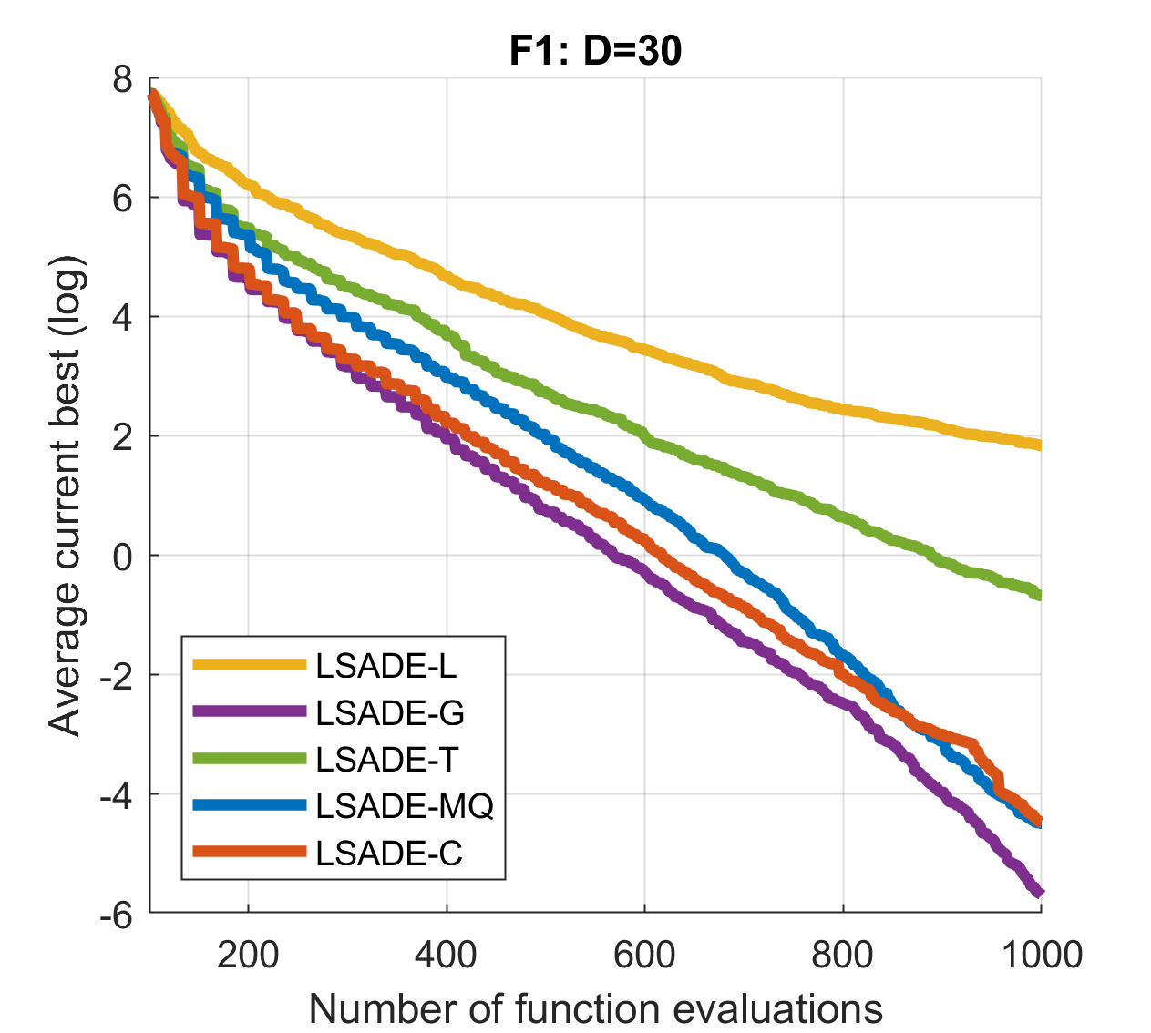
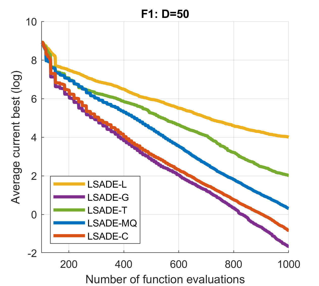
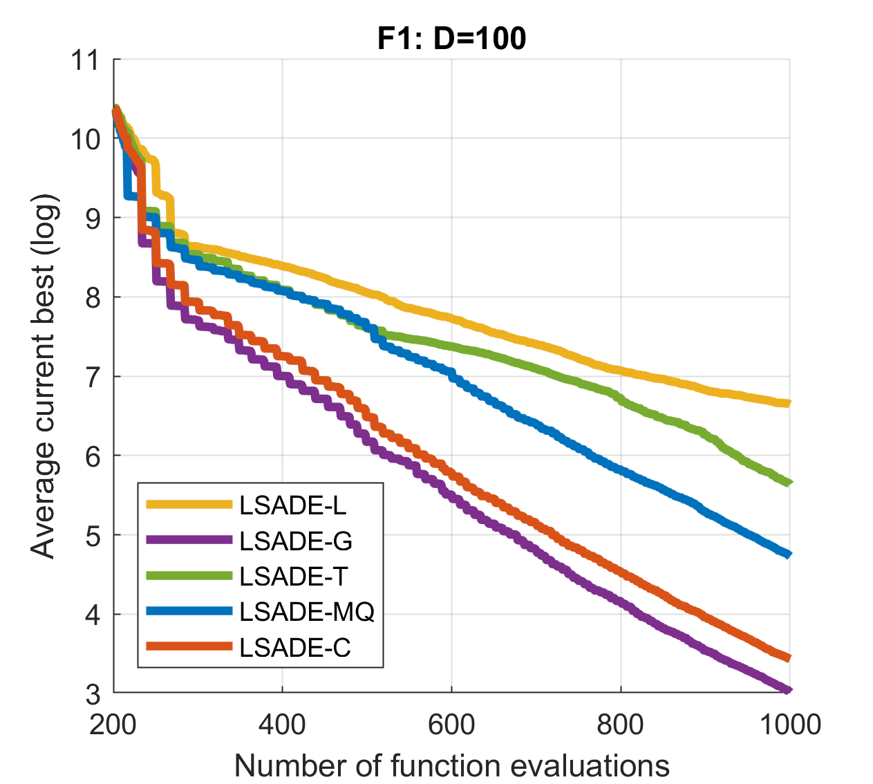
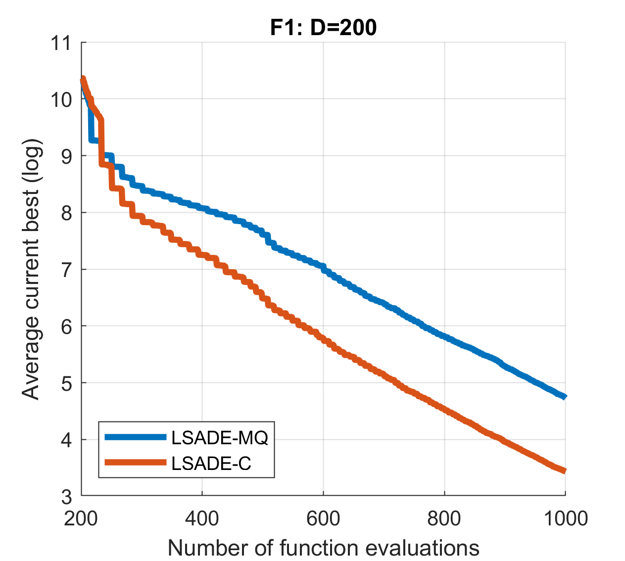
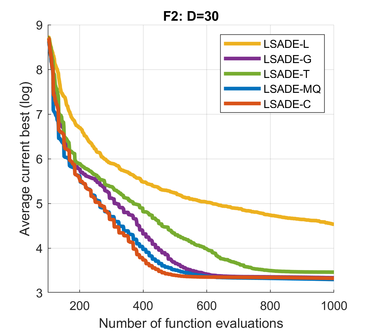
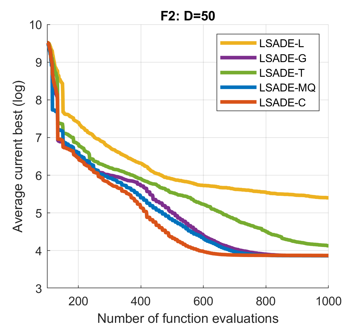
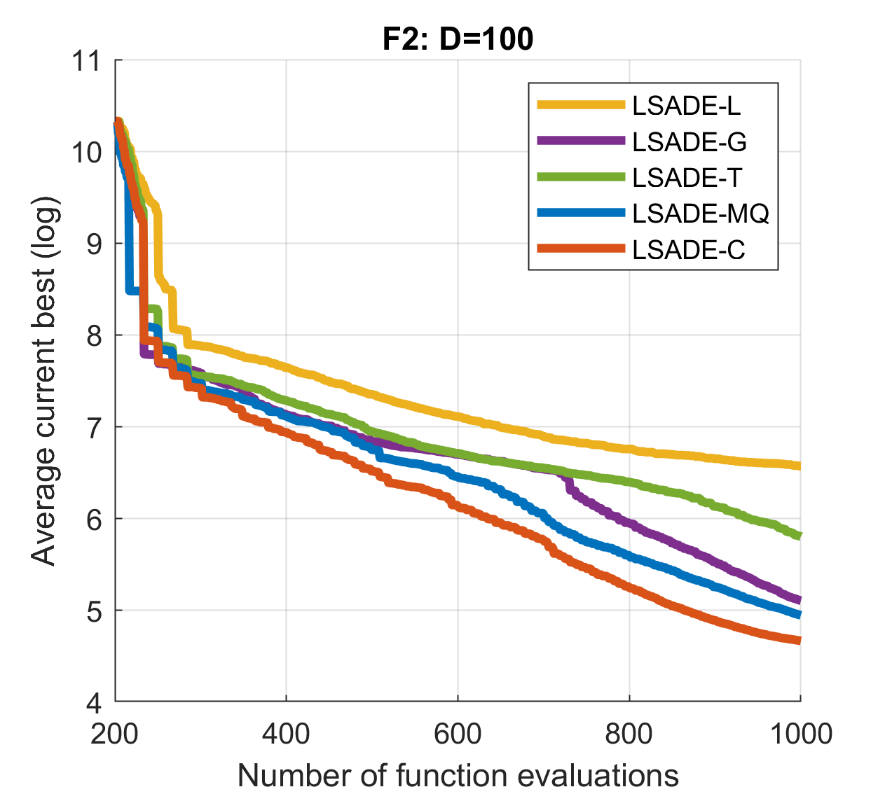
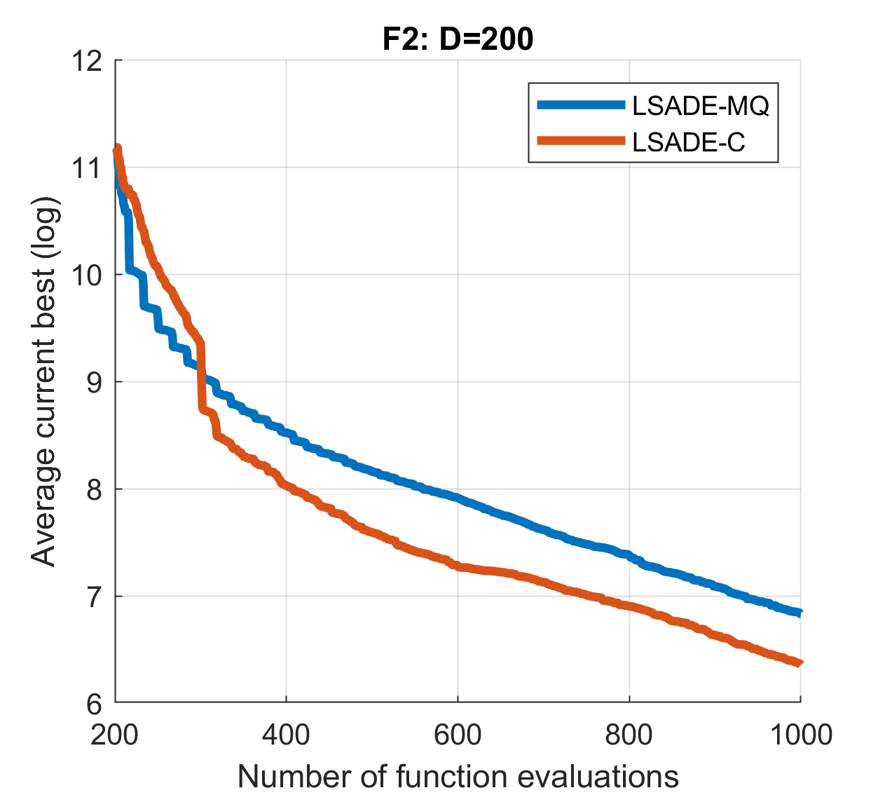
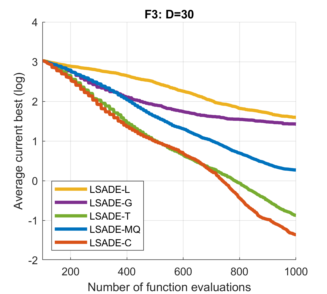
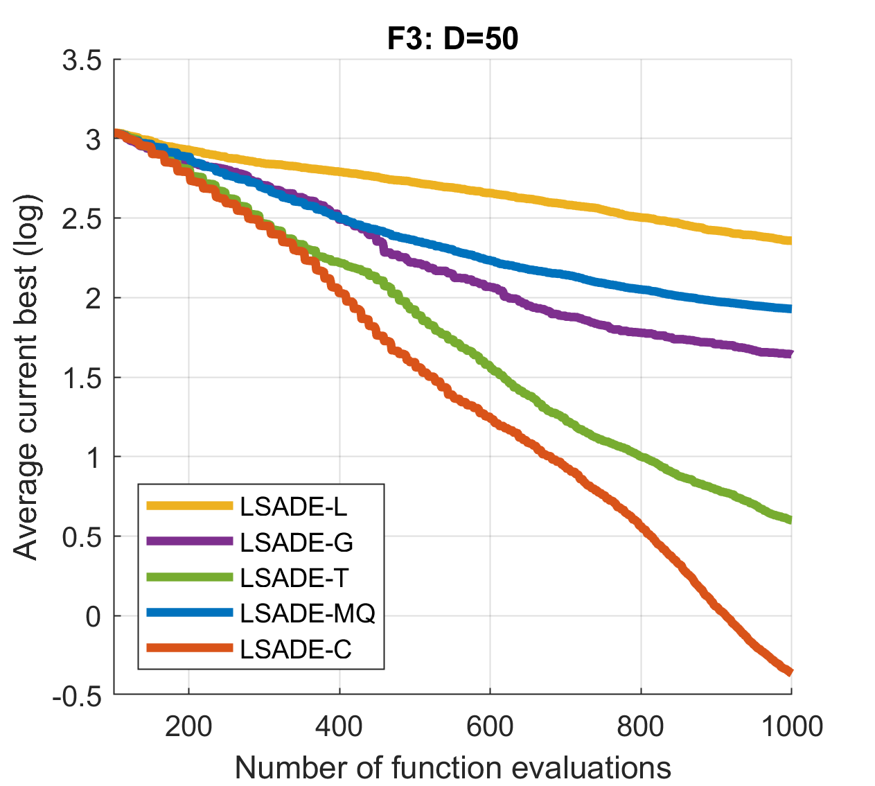
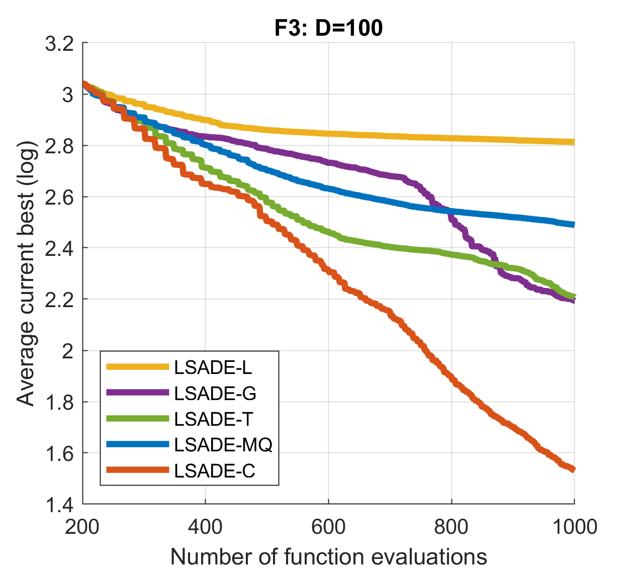
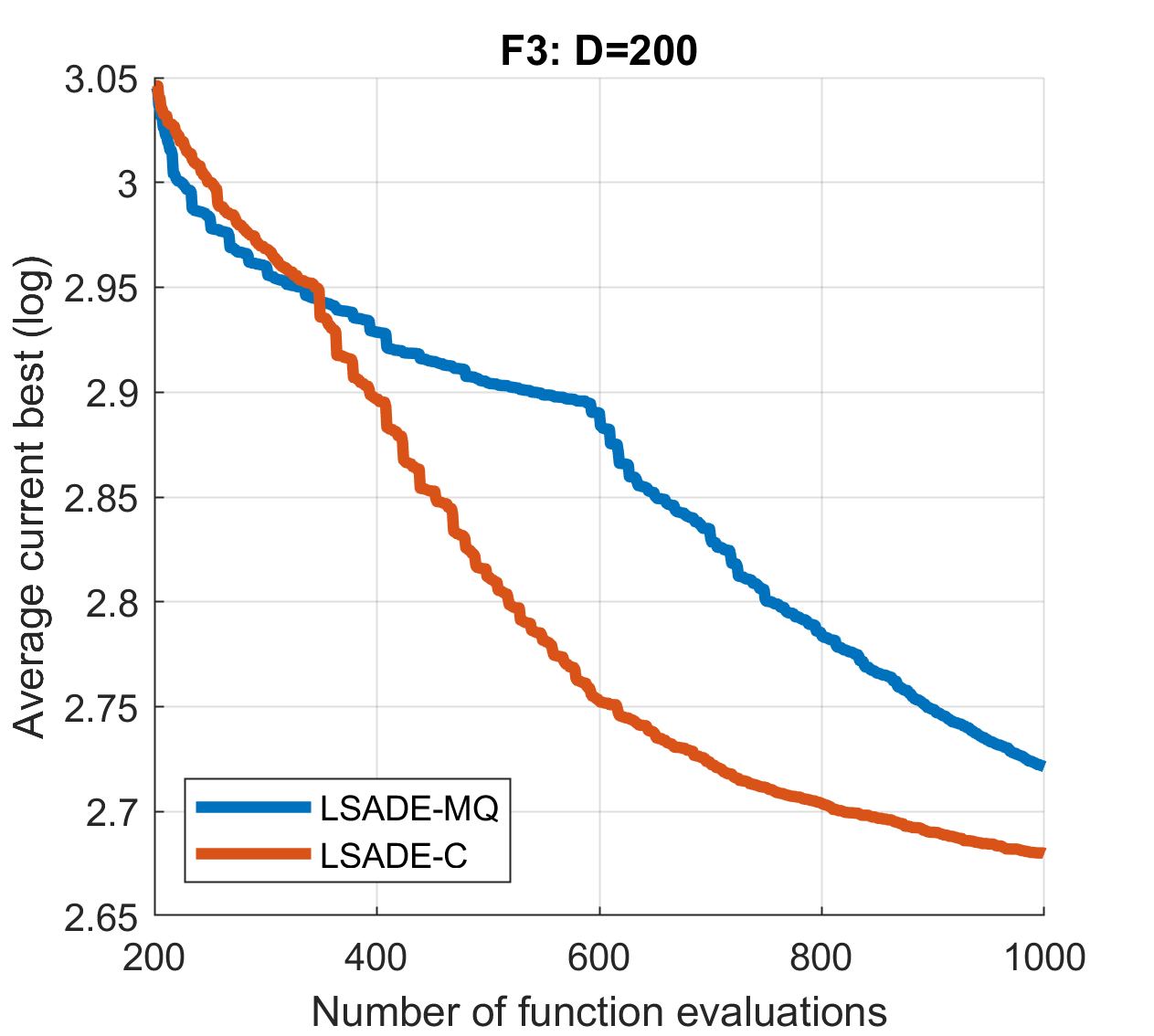
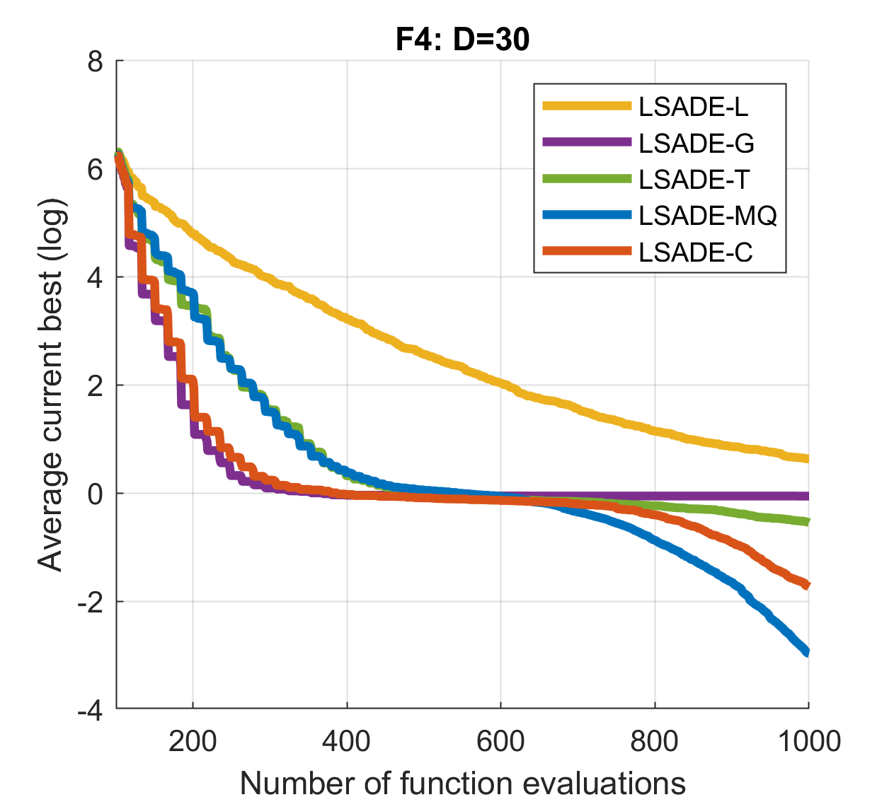
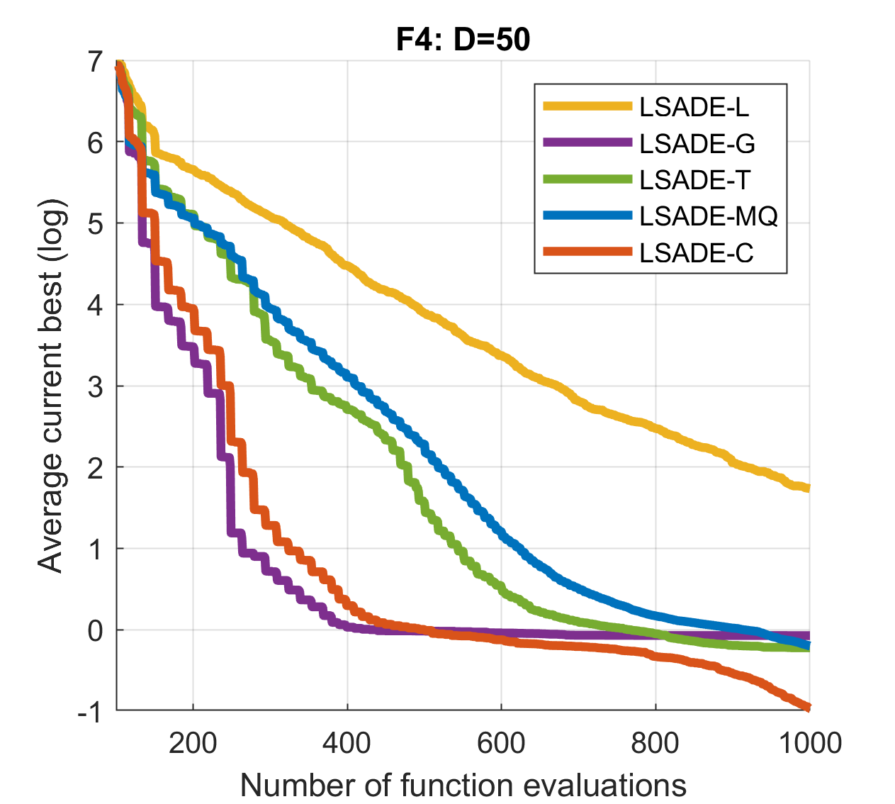
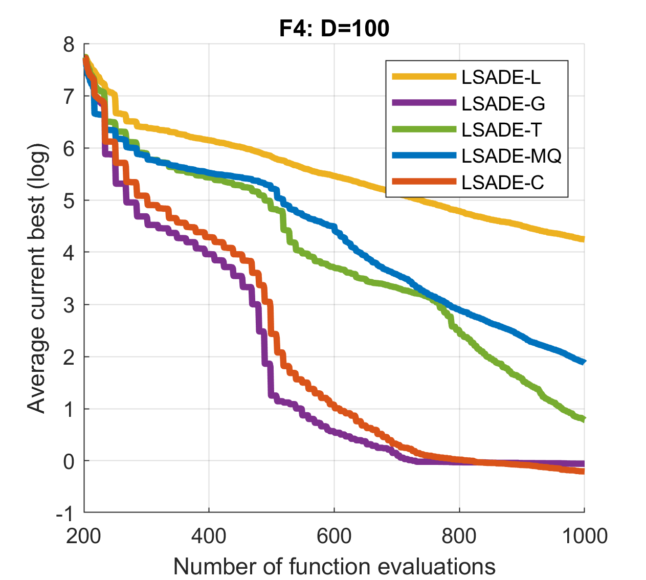
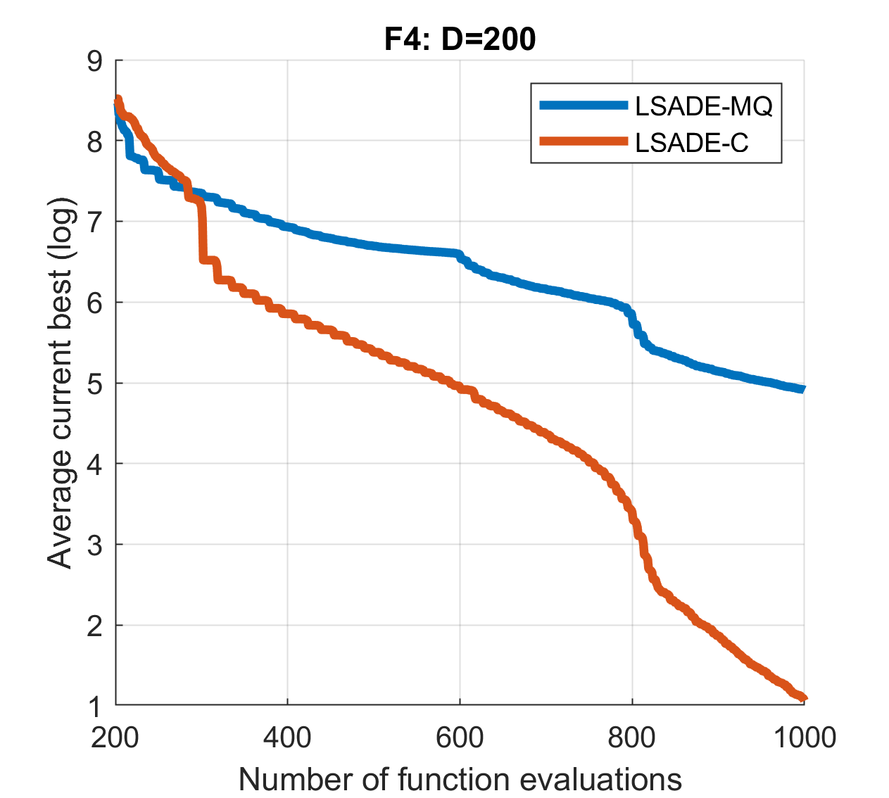
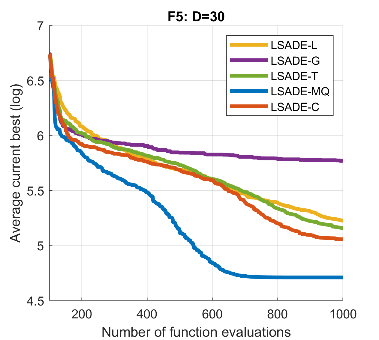
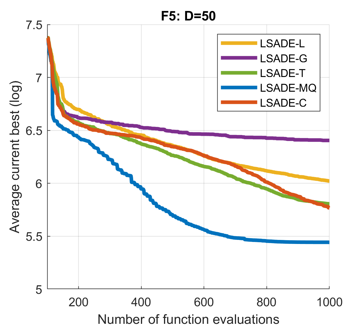
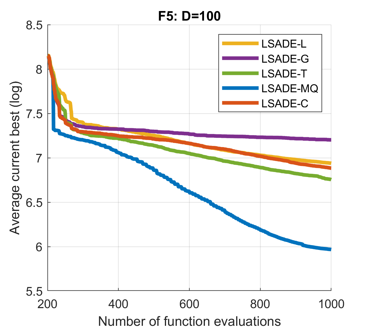
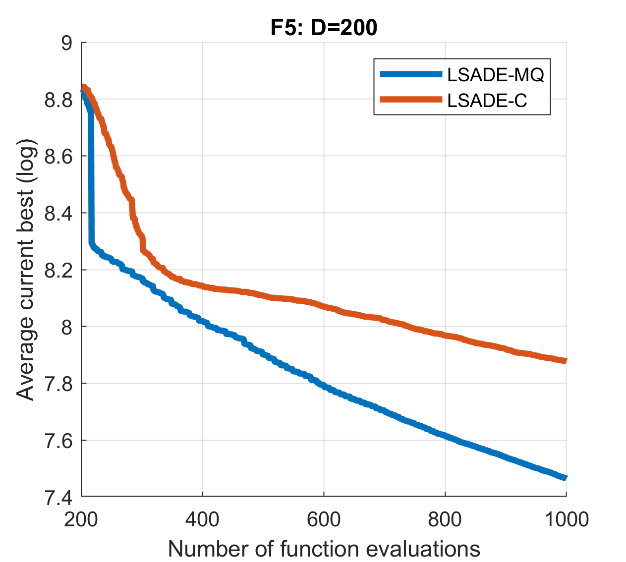
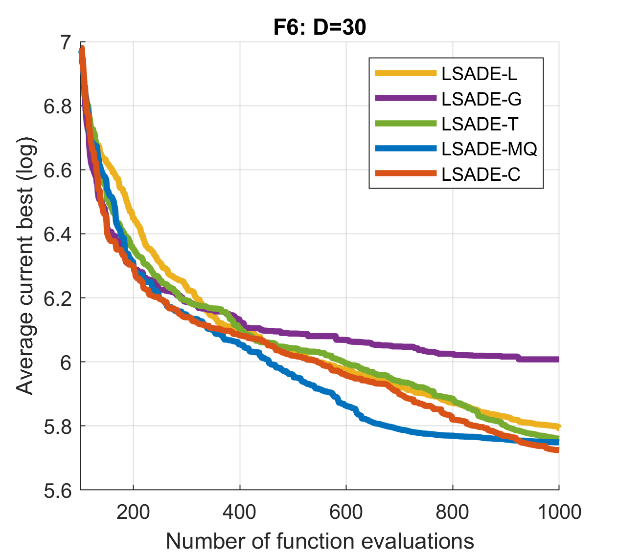
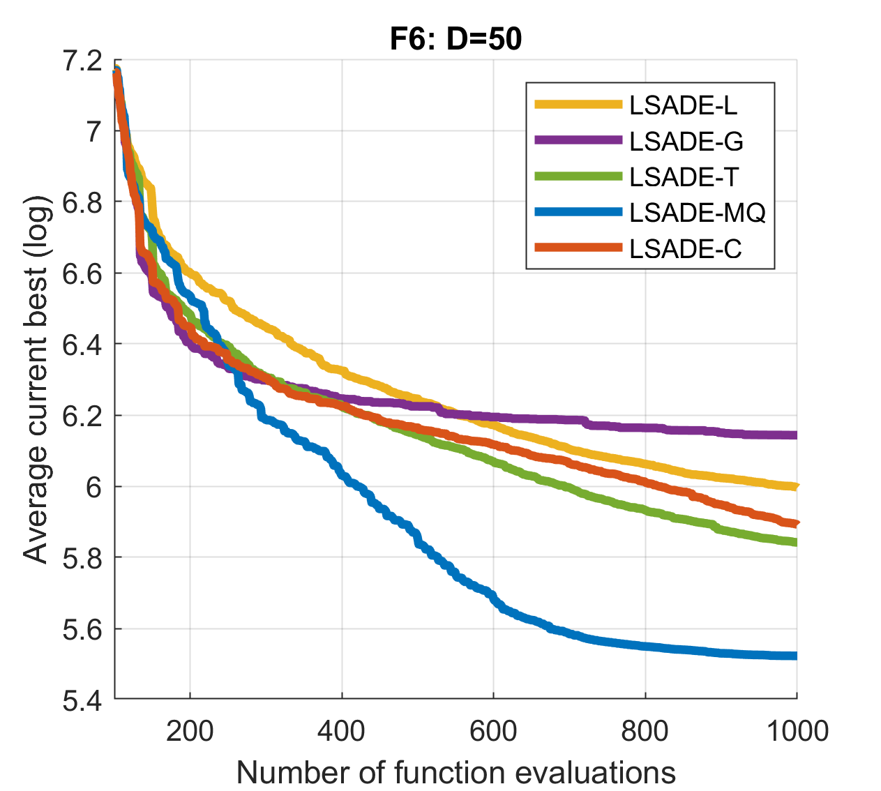
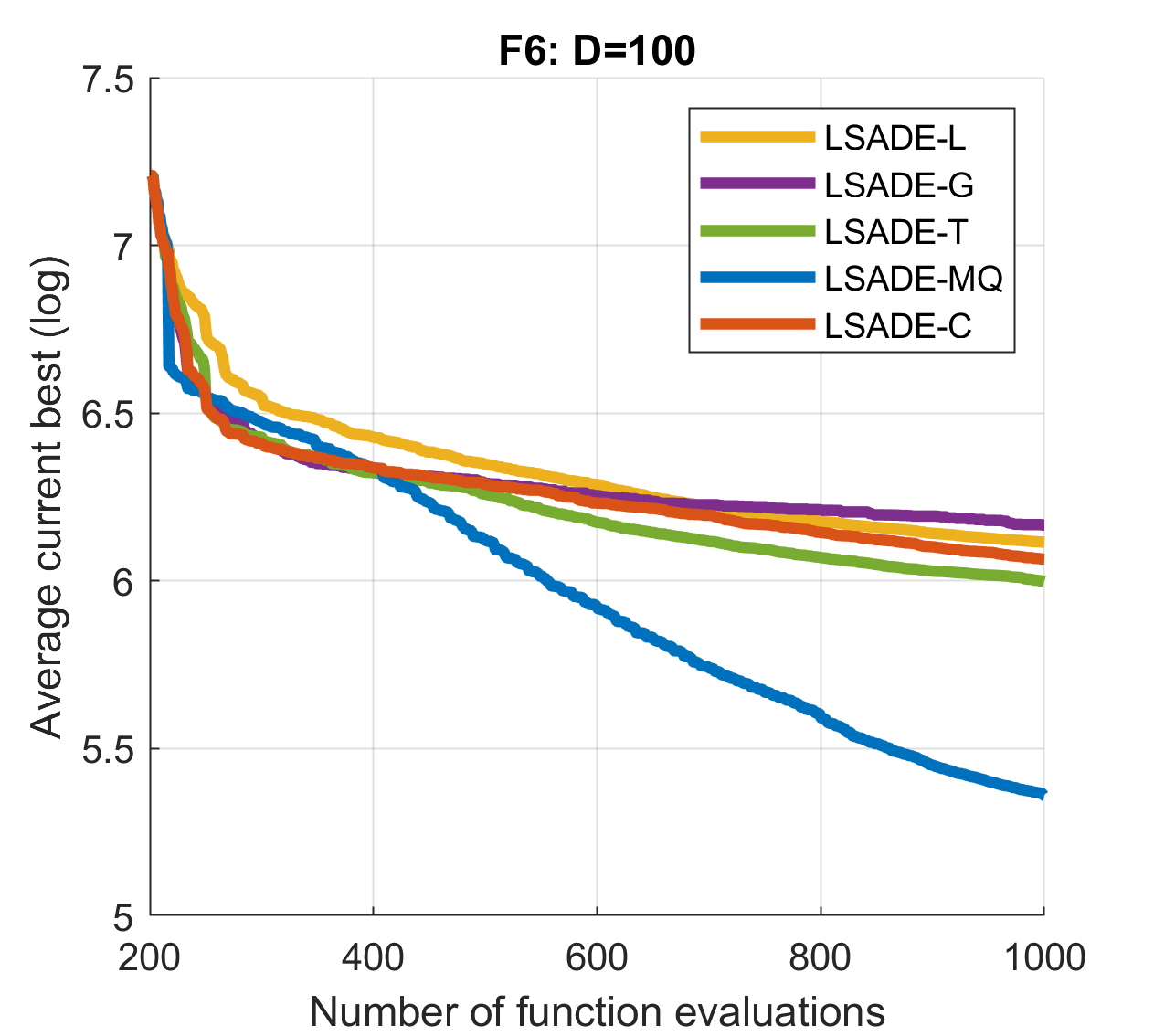
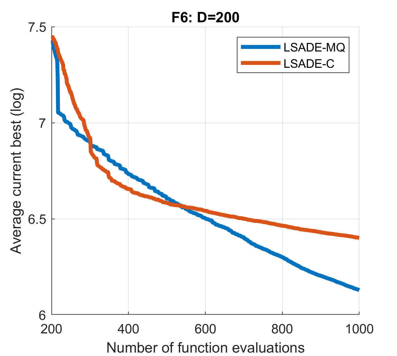
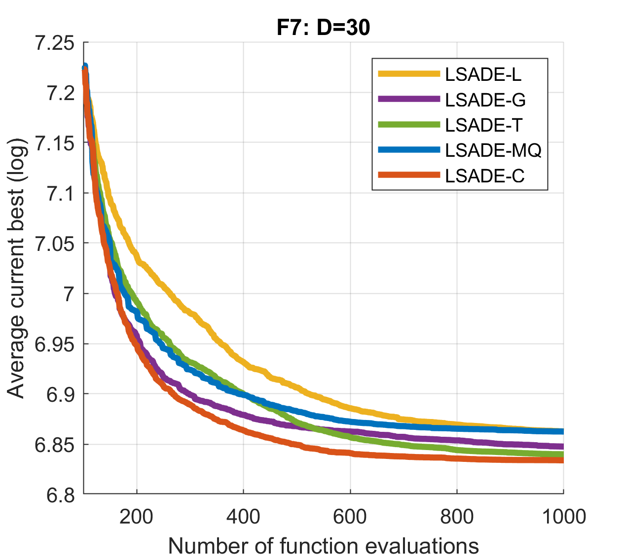
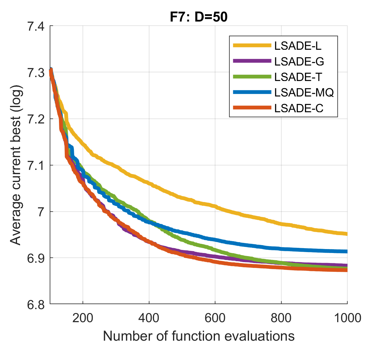
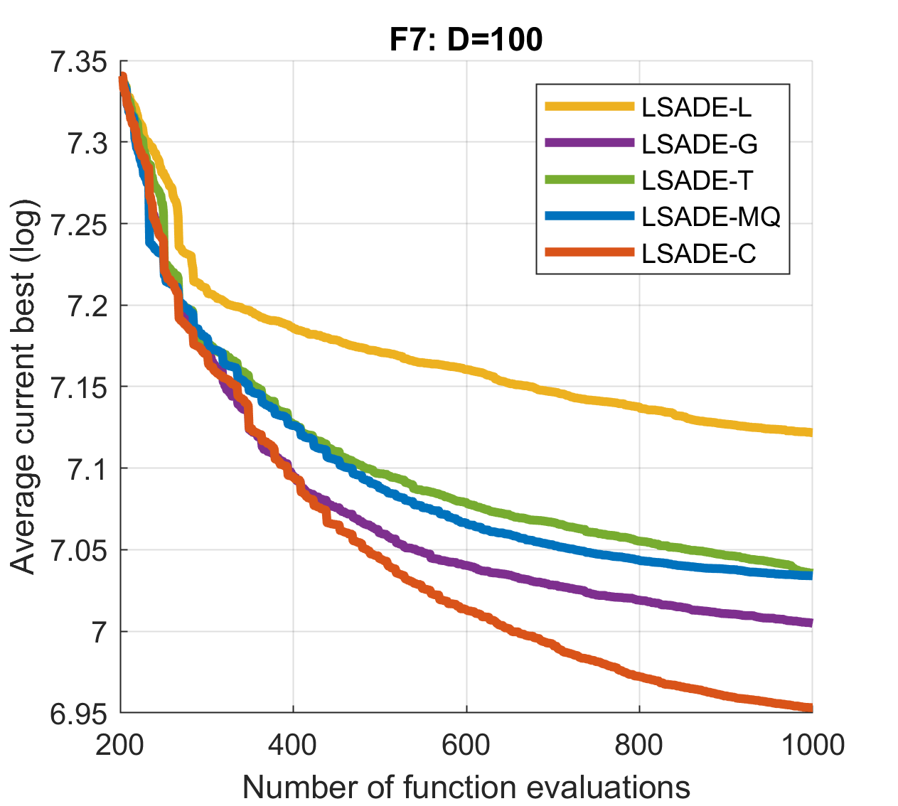
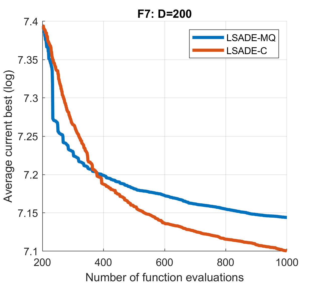
Figure 5: Convergence history of LSADE with different basis functions on the benchmark functions F1–F7 in different dimensions.

Table 16: Detailed statistics of the results for SAMSO, MGP-SLPSO, GSGA, and SAGWO algorithms on all considered benchmark functions.

		SAMSO		MGP-SLPSO				GSGA				SAGWO
$D$	F	mean	std	best	mean	worst	std	best	mean	worst	std	best	mean	worst	std
	F1	0.0053	0.0057	N/A	0	N/A	0	0.0051	0.072	0.326	0.093	0.00001	0.000065	0.0003	0.000075
	F2	28.3	0.854	N/A	100	N/A	22.3	25.69	27.59	29.04	1.295	26.79	28.29	28.83	0.517
	F3	0.628	0.542	N/A	6.58	N/A	2.6	0.0065	0.023	0.057	0.023	0	0	0	0
30	F4	0.538	0.144	N/A	0.013	N/A	0.005	0.095	0.228	0.383	0.222	0.000001	0.015	0.134	0.032
	F5	-239	24.3	N/A	-220	N/A	19.6	-245.2	-203	-159.0	24.87	-176	-128.8	-58.71	30.82
	F6	372	14.7	N/A	N/A	N/A	N/A	275.5	424.7	563.1	106.2	348.4	489.8	675.8	128.8
	F7	922	3.66	N/A	952	N/A	19	918.8	927.2	938.8	6.043	942.5	973.2	1016	18.47
	F1	0.513	0.285	0	0	0	0	0.203	0.621	1.868	0.484	0.0007	0.004	0.015	0.0036
	F2	50.1	0.768	88.4	120	165	18.7	46.84	48.21	49.10	0.766	48.35	49.06	49.94	0.449
	F3	1.53	0.436	7.77	9.31	12.1	1.13	0.0060	0.021	0.076	0.023	0	0	0	0
50	F4	0.666	0.107	0.037	0.154	0.614	0.13	0.272	0.346	0.442	0.071	0.000035	0.025	0.230	0.058
	F5	-169	31.7	-43.4	33	88.4	36.1	-139.6	-75.82	12.09	49.99	-16.63	98.39	161.5	46.90
	F6	326	98.6	N/A	N/A	N/A	N/A	271.8	403.3	524.8	87.59	430.2	502	564.2	45.25
	F7	970	29.2	1030	1060	1110	21.4	943.7	970.7	1002	18.18	910	1044	1132	40.83
	F1	72.1	17.8	0	0.00005	0.001	0.0002	2.603	12.32	27.15	9.394	0.017	0.139	0.371	0.097
	F2	286	52.5	455	612	733	67.9	99.743	109.0	139.3	11.76	104.9	123.4	144.8	11.02
	F3	6.12	0.409	13.4	14.3	15.7	0.621	0.156	1.31	2.807	0.968	0	0	0	0
100	F4	1.06	0.026	0.478	0.715	0.847	0.724	0.580	0.706	0.804	0.070	0.00021	0.023	0.229	0.052
	F5	737	42	877	885	1160	117	620.4	672.5	705.2	29.79	676.7	800.1	919.0	79.27
	F6	513	18.5	N/A	N/A	N/A	N/A	422.4	447.2	472.6	14.25	482.0	518.6	555.3	20.54
	F7	1290	33.4	1330	1390	1490	47.7	1220	1256	1287	24.56	910.2	1350	1437	107.5
	F1	1520	21.2	N/A	N/A	N/A	N/A	N/A	N/A	N/A	N/A	N/A	N/A	N/A	N/A
	F2	1150	11.6	N/A	N/A	N/A	N/A	N/A	N/A	N/A	N/A	N/A	N/A	N/A	N/A
	F3	12	0.4	N/A	N/A	N/A	N/A	N/A	N/A	N/A	N/A	N/A	N/A	N/A	N/A
200	F4	9.03	1.33	N/A	N/A	N/A	N/A	N/A	N/A	N/A	N/A	N/A	N/A	N/A	N/A
	F5	4960	138	N/A	N/A	N/A	N/A	N/A	N/A	N/A	N/A	N/A	N/A	N/A	N/A
	F6	684	37.2	N/A	N/A	N/A	N/A	N/A	N/A	N/A	N/A	N/A	N/A	N/A	N/A
	F7	1340	24.3	N/A	N/A	N/A	N/A	N/A	N/A	N/A	N/A	N/A	N/A	N/A	N/A

Table 17: Detailed statistics of the results for EASO, SA-COSO, LSADE-MQ, and LSADE-C algorithms on all considered benchmark functions.

		EASO		SA-COSO		LSADE-MQ				LSADE-C
$D$	F	mean	std	mean	std	best	mean	worst	std	best	mean	worst	std
	F1	0.027	0.070	3.85	1.19	0.0039	0.011	0.021	0.005	0.0008	0.011	0.047	0.012
	F2	25.04	1.57	59.9	24.3	24.31	27.06	29.35	1.243	27.20	27.77	29.36	0.546
	F3	2.521	0.84	5.01	1.22	0.026	1.308	3.028	1.011	0.0025	0.256	1.186	0.441
30	F4	0.953	0.05	1.44	0.18	0.0098	0.051	0.107	0.027	0.046	0.176	0.673	0.172
	F5	6.325	26.5	-57.4	17.5	-278.2	-218.7	-136.0	35.68	-256.2	-172.6	-81.31	39.83
	F6	N/A	N/A	528	94.8	229.2	433.7	664.1	149.3	233.5	426.2	674.3	148.1
	F7	931.6	8.94	969	24.3	922.2	965.7	1097	51.86	916.1	938.8	1004.3	26.37
	F1	0.740	0.555	46.6	17.4	0.265	1.358	3.500	0.860	0.047	0.433	1.304	0.299
	F2	47.39	1.71	253	56.7	43.92	47.65	49.17	1.332	45.53	47.98	49.19	0.864
	F3	1.431	0.249	8.86	1.1	2.615	6.876	15.39	3.456	0.029	0.695	2.264	0.600
50	F4	0.94	0.042	5.63	0.892	0.560	0.819	1.051	0.132	0.198	0.38	0.662	0.129
	F5	198.6	45.8	235	40.9	-194.6	-98.78	-5.288	52.92	-183.0	-10.03	151.2	93.88
	F6	N/A	N/A	613	37.4	259.0	370.3	579.8	109.5	339.2	481.6	657.1	80.89
	F7	975.3	37.1	1080	36.6	954.3	1016	1134	53.369	936.1	976.3	1103	38.52
	F1	1283	134	985	214	58.02	112.8	171.2	33.61	12.93	30.94	61.73	12.46
	F2	578.8	44.8	2500	97.4	108.3	140.6	194.3	24.10	97.62	106.4	120.8	6.631
	F3	10.36	0.211	15.9	0.514	9.431	12.05	16.54	2.203	3.540	4.622	6.157	0.619
100	F4	57.34	5.84	63.5	14.9	3.344	6.517	10.04	1.974	0.694	0.816	0.923	0.059
	F5	713.4	26.5	1420	123	-71.63	60.28	426.2	121.0	503.0	646.8	768.0	64.37
	F6	N/A	N/A	807	65.7	267.3	332.7	419.4	37.77	486.8	550.4	688.2	43.30
	F7	1372	27.5	1410	22.8	1076	1144	1232	44.45	1002	1056	1146	34.27
	F1	17616	1170	16382	2980	2473	3959	5192	705.2	587.6	793.5	1137	154.3
	F2	4318	284	16411	4100	683.0	927.2	1087	112.4	507.3	576.3	662.5	46.35
	F3	14.69	0.219	17.86	0.022	13.97	15.2	16.08	0.509	11.59	14.58	17.30	1.400
200	F4	572.9	36	577.7	101	93.89	135.6	188.2	22.05	2.149	2.892	3.456	0.394
	F5	5389	157	3927	27.3	1114	1416	2034	287.1	2042	2305	2625	156.8
	F6	N/A	N/A	N/A	N/A	474.5	578.7	883.3	88.76	541.2	722.7	818.7	60.65
	F7	1456	20.4	1347	24.7	1226	1276	1352	28.15	1140	1222	1274	33.38

References

- (1) Y. Jin and B. Sendhoff, “A systems approach to evolutionary multiobjective structural optimization and beyond,” IEEE Comput. Intell. Mag., vol. 4, no. 3, pp. 62–76, 2009.
- (2) M. Emmerich, A. Giotis, M. Özdemir, T. Bäck, and K. Giannakoglou, “Metamodel—Assisted evolution strategies,” in Parallel Problem Solving From Nature—PPSN. Heidelberg, Germany: Springer, 2002, pp. 361–370.
- (3) Y. Jin, H. Wang, T. Chugh, D. Guo, and K. Miettinen, “Data-Driven Evolutionary Optimization: An Overview and Case Studies”, IEEE Trans. Evol. Comp., vol. 23, no. 3, pp. 442–458, 2019.
- (4) Y. Jin, “Surrogate-assisted evolutionary computation: Recent advances and future challenges,” Swarm Evol. Comput., vol. 1, no. 2, pp. 61–70, 2011.
- (5) R. H. Myers and D. C. Montgomery, Response Surface Methodology: Process and Product in Optimization Using Designed Experiments. New York, NY, USA: Wiley, 1995.
- (6) J. D. Martin and T. W. Simpson, “Use of Kriging models to approximate deterministic computer models,” AIAA J., vol. 43, no. 4, pp. 853–863, 2005.
- (7) Y. Jin and B. Sendhoff, “Reducing fitness evaluations using clustering techniques and neural network ensembles,” in Proc. Genet. Evol. Comput. Conf., Seattle, WA, USA, 2004, pp. 688–699.
- (8) N. Dyn, D. Levin, and S. Rippa, “Numerical procedures for surface fitting of scattered data by radial functions,” SIAM J Sci. Stat. Comput., vol. 7, no. 2, pp. 639–659, 1986.
- (9) S. R. Gunn, “Support vector machines for classification and regression,” Dept. Electron. Comput. Sci., Univ. Southampton, Southampton, U.K., Rep., 1998.
- (10) R. Jin, W. Chen, T. W. Simpson, “Comparative studies of metamodelling techniques under multiple modelling criteria,” Struct. Multidiscipl. Optim., vol. 23, no. 1, pp. 1–13, 2001.
- (11) S. R. Young, D. C. Rose, T. P. Karnowski, S. H. Lim, and R. M. Patton, “Optimizing deep learning hyper-parameters through an evolutionary algorithm,” in Proceedings of the workshop on machine learning in high-performance computing environments, pp. 1–5, 2015.
- (12) R. Matousek, P. Popela, and J. Kudela, “Heuristic approaches to stochastic quadratic assignment problem: Var and cvar cases,” MENDEL, vol. 23, pp. 73–78, 2017.
- (13) P. Zufan, and M. Bidlo, “Advances in evolutionary optimization of quantum operators,” MENDEL, vol. 27, no. 2, pp. 12–22, 2021.
- (14) Z. Abo-Hammour, O. Alsmadi, S. Momani, and O. A. Arqub, “A Genetic Algorithm Approach for Prediction of Linear Dynamical Systems,” Mathematical Problems in Engineering, vol. 2013, Article ID 831657, 2013.
- (15) O. A. Arqub, and Z. Abo-Hammour, “Numerical solution of systems of second-order boundary value problems using continuous genetic algorithm,” Information Sciences, vol. 279, pp. 396–415, 2014.
- (16) H. Rakhshani, L. Idoumghar, J. Lepagnot, and M. Brévilliers, “Speed up differential evolution for computationally expensive protein structure prediction problems,” Swarm and Evolutionary Computation, vol. 50, paper ID 100493, 2019.
- (17) H. Dong, X. Li, Z. Yang, L. Gao, and Y. Lu, “A two-layer surrogate-assisted differential evolution with better and nearest option for optimizing the spring of hydraulic series elastic actuator,” Applied Soft Comp., vol. 100, paper ID 107001, 2021.
- (18) D. Wang, Z. Wu, Y. Fei, and W. Zhang, “Structural design employing a sequential approximation optimization approach,” Comput. Struct., vol. 134, pp. 75–87, 2014.
- (19) S. Wang, J. Liu, and Y. Jin, “Surrogate-Assisted Robust Optimization of Large-Scale Networks Based on Graph Embedding,” IEEE Trans. Evol. Comp., vol. 24, no. 4, pp. 735–749, 2020.
- (20) J. Kudela, and R. Matousek, “Recent Advances and Applications of Surrogate Models for Finite Element Method Computations: A Review ”, Soft Computing, 2022, doi: 10.1007/s00500-022-07362-8.
- (21) R. G. Regis, “Particle swarm with radial basis function surrogates for expensive black-box optimization,” J. Comp. Sci., vol. 5, pp. 12–23, 2014.
- (22) C. Sun, Y. Jin, J. Zeng, and Y. Yu, “A two-layer surrogate-assisted particle swarm optimization algorithm,” Soft Comput., vol. 19, no. 6, pp. 1461–1475, 2014.
- (23) B. Liu, Q. Zhang, and G. G. E. Gielen, “A Gaussian process surrogate model assisted evolutionary algorithm for medium scale expensive optimization problems,” IEEE Trans. Evol. Comp., vol. 18, no. 2, pp. 180–192, 2014.
- (24) F. Li, X. Cai, and L. Gao, “Ensemble of surrogates assisted particle swarm optimization of medium scale expensive problems,” Appl. Soft Comput., vol. 74, pp. 291–305, 2019.
- (25) Y. S. Ong, P. B. Nair, and A. J. Keane, “Evolutionary optimization of computationally expensive problems via surrogate modeling,” AIAA J., vol. 41, no. 4, pp. 687–696, 2003.
- (26) C. Sun, Y. Jin, R. Cheng, J. Ding, and J. Zeng, “Surrogate-Assisted Cooperative Swarm Optimization of High-Dimensional Expensive Problems,” IEEE Trans. Evol. Comp., vol. 21, no. 4, pp. 644–660, 2017.
- (27) H. Wang, “Uncertainty in surrogate models,” in Proc. ACM Genet. Evol. Comput. Conf., 2016, p. 1279.
- (28) D. Lim, Y. Jin, Y.-S. Ong, and B. Sendhoff, “Generalizing surrogateassisted evolutionary computation,” IEEE Trans. Evol. Comp., vol. 14, no. 3, pp. 329–355, 2010.
- (29) R. Mallipeddi and M. Lee, “An evolving surrogate model-based differential evolution algorithm,” Appl. Soft Comp., vol. 34, pp. 770–787, 2015.
- (30) X. G. Zhou, and G. J. Zhang, “Abstract convex underestimation assisted multistage differential evolution,” IEEE transactions on cybernetics, vol. 47, no. 9, pp. 2730–2741, 2017.
- (31) F. Li, X. Cai, L. Gao, and W. Shen, “A surrogate-assisted multi-swarm optimization algorithm for high-dimensional computationally expensive problems,” IEEE Trans. Cyber., vol. 51, pp. 1390–1402, 2021.
- (32) H. Wang, Y. Jin, and J. Doherty, “Committee-based active learning for surrogate-assisted particle swarm optimization of expensive problems,” IEEE Trans. Cybern., vol. 47, pp. 2664–2677, 2017.
- (33) X. Wang , G. G. Wang, B. Song, P. Wang, and Y. Wang, “A Novel Evolutionary Sampling Assisted Optimization Method for High-Dimensional Expensive Problems,” IEEE Trans. Evol. Comput., vol. 23, no. 5, pp. 815–827, 2019.
- (34) X. Cai, L. Gao, and X. Li, “Efficient Generalized Surrogate-Assisted Evolutionary Algorithm for High-Dimensional Expensive Problems,” IEEE Trans. Evol. Comp., vol. 24, pp. 365–379, 2020.
- (35) J. Tian, Y. Tan, J. Zeng, C. Sun, Y. Jin, “Multiobjective Infill Criterion Driven Gaussian Process-Assisted Particle Swarm Optimization of High-Dimensional Expensive Problems,” IEEE Trans. Evol. Comp., vol. 23, pp. 459–472, 2019.
- (36) H. Dong and Z. Dong, “Surrogate-assisted grey wolf optimization for high-dimensional, computationally expensive black-box problems,” Swarm Evol. Comput., vol. 57, article no. 100713, 2020.
- (37) A. I. J. Forrester and A. J. Keane, “Recent advances in surrogate-based optimization,” Progr. Aerosp. Sci., vol. 45, nos. 1–3, pp. 50–79, 2009.
- (38) A. Díaz-Manríquez, G. Toscano, and C. A. C. Coello, “Comparison of metamodeling techniques in evolutionary algorithms,” Soft. Comput., vol. 21, pp. 5647–5663, 2017.
- (39) S. A. Piyavskii, “An algorithm for finding the absolute extremum of a function,” USSR Computational Mathematics and Mathematical Physics, vol. 12, no. 4, pp. 57–67, 1972.
- (40) B. O. Shubert, “A sequential method seeking the global maximum of a function,” SIAM Journal on Numerical Analysis, vol. 9, no. 3, pp. 379–388, 1972.
- (41) C. Malherbe and N. Vayatis, “Global optimization of Lipschitz functions,” arXiv, arXiv:1703.02628, 2017.
- (42) S. Das and P. N. Suganthan, “Differential evolution: a survey of the state-of-the-art,” IEEE Trans. Evol. Comp., vol. 15, no. 1, pp. 4–31, 2011.
- (43) R. Matousek, L. Dobrovsky, and J. Kudela, “How to start a heuristic? utilizing lower bounds for solving the quadratic assignment problem,” International Journal of Industrial Engineering Computations vol. 13, no. 2, pp. 151–164, 2022.
- (44) K. M. Sallam, S. M. Elsayed, R. K. Chakrabortty, and M. J. Ryan, “Improved Multi-operator Differential Evolution Algorithm for Solving Unconstrained Problems,” 2020 IEEE Congress on Evolutionary Computation (CEC), paper no. 19931315, 2020.
- (45) P. Suganthan, N. Hansen, J. Liang, K. Deb, Y.-P. Chen, A. Auger, and S. Tiwari, “Problem definitions and evaluation criteria for the CEC 2005 special session on real-parameter optimization,” Nat. Comput., pp. 341–357, 2005.
- (46) J. Kudela, and R. Matousek, “New Benchmark Functions for Single-Objective Optimization Based on a Zigzag Pattern,” IEEE Access, vol. 10, 8262–8278, 2022.
- (47) F. A. C. Viana. (2011). SURROGATES Toolbox User’s Guide, Version 3.0. [Online]. Available: http://sites.google.com/site/felipeacviana/surrogatestoolbox
- (48) A. Kazikova, M. Pluhacek, and R. Senkerik, “Why tuning the control parameters of metaheuristic algorithms is so important for fair comparison?,” MENDEL, vol. 26, no. 2, pp. 9–16, 2020.