Reduction of Stratified Axi-Symmetric Euler-Poisson Equations Under Symmetry

Abstract

The paper considers Euler-Poisson equations which govern the steady state of a self gravitating, rotating, axi-symmetric fluid under the additional assumption that it is incompressible and stratified. In this setting we show that the original system of six nonlinear partial differential equations can be reduced to two equations, one for the mass density and the other for gravitational field. This reduction is carried out in cylindrical coordinates. As a result we are able to derive also expressions for the pressure as a function of the density. The resulting equations are then solved analytically. These analytic solutions are used then to determine the shape of the rotating star (or interstellar cloud) by applying the boundary condition that the pressure is zero at the boundary.

1 Introduction

The steady states of self gravitating fluid in three dimensions have been studied by a long list of theoretical physicists and astrophysicists. (For an extensive list of references see [2, 3, 18, 19, 25, 26]. In fact research related to this problem persists even today [11, 16, 17, 22, 23, 24, 21]. The motivation for this research is due to the interest in the formation, shape, and stability of stars and other celestial bodies.

Within the context of classical mechanics attempts to describe star interiors are based on Euler-Poisson equations [2, 3]. Well known solutions to these equations are the Lane-Emden functions, which describe static steady state of non-rotating spherically symmetric fluid with mass-density $\rho=\rho(r)$ and flow field $\bf u=0$. The generalization of these equations to include axi-symmetric rotations was considered by Milne[19], Chandrasekhar[2, 3], and many others [14, 13, 19, 20]. One of difficulties in the treatment of this problem is due to the fact that the boundary of the domain can not be prescribed apriori, and one has to address a free boundary problem. An approximate treatment of this problem for polytropic stars in spherical coordinates was made in the seminal paper by Roxburgh[24]. Other treatments which considered different aspects of this problem appeared in the literature since then [1, 4, 11, 12, 14, 23].

In a previous paper [7] on this topic, we addressed the steady states of non-rotating self gravitating incompressible fluid with axial symmetry. In the present paper, we generalize this treatment and address the modeling of axi-symmetric rotating fluids. To do so we add the assumption that the mass-density is stratified [5, 6, 7, 8, 10, 18, 25, 26] to the Euler-Poisson equations with axi-symmetric rotations. Under these assumptions we show that the number of model equations for the (non static) steady state can be reduced from six to a system of two coupled equations. One for the mass-density and the second for the gravitational field. These equations contain, however, a parameter function $h(\rho)$ that encode the information about the momentum distribution within the star. This reduction in the number of model equations (in this settings) may be used to obtain new insights for the treatment of this problem and make it tractable both analytically and numerically. We provide in this paper analytic and numerical solutions to these equations and apply these solutions to solve for the shape of an axi-symmetric rotating star.

It might be argued that Euler-Poisson equations do not actually hold in a star interior due to the various physical processes taking place there (e.g turbulence, radiation, compressibility, etc)[9]. Nevertheless they provide a natural extension to the results on the equilibrium states of three dimensional bodies under gravity.

The plan of the paper is as follows: In Sec. $2$, we present the basic model equations. In Sec. $3$, we carry out, in cylindrical coordinates, the reduction of these model equations from six to two. (similar reduction can be carried out in spherical coordinates). We provide also expressions for the pressure in this coordinate system. In Secs. $4$ and $5$, we derive analytic solutions to these equations and discuss the shape of the rotating star (or interstellar cloud) by applying the boundary condition that the pressure is zero on the boundary. We end up in Sec. $6$, with summary and conclusions.

2 Derivation of the Model Equations

In this paper we consider the state of an inviscid incompressible stratified self gravitating fluid. In addition we assume that the fluid it is subject to axial rotations. The hydrodynamic equations that govern this flow in an inertial frame of reference are [1, 2, 5, 8, 20, 25];

$$\nabla\cdot{\bf v}=0$$ (2.1)

$${\bf v}\cdot\nabla\rho=0$$ (2.2)

$$\frac{1}{2}\rho\nabla({\bf v}\cdot{\bf v})+\rho(\nabla\times{\bf v})\times{\bf v}=-\nabla p-\rho\nabla\Phi$$ (2.3)

$$\nabla^{2}\Phi=4\pi G\rho$$ (2.4)

where ${\bf v}=(u,v,w)$ is the fluid velocity, $\rho$ is its density $p$ is the pressure, $\Phi$ is the gravitational potential, G is the gravitational constant, and the momentum equations (2.3) are written in Lambs’s form. Subscripts denote differentiation with respect to the indicated variable.

We can nondimensionalize these equations by introducing the following scalings

$$x=L\tilde{x},\,\,\ y=L\tilde{y},\,\,\,z=L\tilde{z},\,\,\,{\bf v}=U_{0}\tilde{{\bf v}},\,\,$$ (2.5)

$$\rho=\rho_{0}\tilde{\rho},\,\,\ p=\rho_{0}U_{0}^{2}\tilde{p},\,\,\,\Phi=U_{0}^{2}\tilde{\Phi},\,\,\,\omega=\frac{U_{0}}{L}\tilde{\omega}.$$

where $L,U_{0},\rho_{0}$ are some characteristic length, velocity, and mass density respectively that characterize the problem at hand.

Substituting these scalings in (2.1)-(2.4) and dropping the tildes, these equations remain unchanged (but the quantities that appear in these equations become nondimensional) while $G$ is replaced by $\tilde{G}=\frac{G\rho_{0}L^{2}}{U_{0}^{2}}$. (Once again we drop the tilde).

We now restrict our discussion to bodies which are axi-symmetric. Without loss of generality, we shall assume henceforth that this axis of symmetry coincides with the z-axis. Under this assumption, it is expeditious to treat the flow in cylindrical (or spherical) coordinate system. In standard cylindrical coordinates $(r,\theta,z)$, we then have (due the symmetry) ${\bf v}={\bf v}(r,z)$, i.e. the flow and the other functions that appear in (2.1)-(2.4) are independent of the angle $\theta$.

We note that all functions in this paper will be assumed to be smooth. Furthermore for the rest of this paper we exclude from our discussion the exceptional cases where $\rho$ is constant or ${\bf v}={\bf 0}$. To determine the shape of a star under these assumptions we impose the boundary condition $p=0$ ([25] p. $54$ and p. $121$). In addition $\rho$ must (obviously) satisfy $\rho\geq 0$.

3 Reduction in Cylindrical Coordinates

Following the standard notation we introduce the frame

$${\bf e}_{r}=(\cos\theta,\sin\theta,0),\,\,\,{\bf e}_{\theta}=(-sin\theta,\cos\theta,0),\,\,\,{\bf e}_{z}=(0,0,1).$$

In this frame we have under present assumptions

$${\bf v}=u(r,z){\bf e}_{r}+w(r,z){\bf e}_{z}+v(r,z){\bf e}_{\theta}={\bf u}(r,z)+v(r,z){\bf e}_{\theta}$$ (3.1)

The momentum equations for ${\bf u}$ can be written as

$$\rho{\bf u}\cdot\nabla{\bf u}=-\nabla p-\rho\nabla\Phi+\rho\frac{v^{2}}{r}{\bf e}_{r}.$$ (3.2)

The equation for $v$ is

$${\bf u}\cdot\nabla v+\frac{uv}{r}=0.$$ (3.3)

We observe also that we can replace ${\bf v}$ by ${\bf u}$ in (2.1)-(2.2).

In the cylindrical coordinate system the continuity equation (2.1) becomes

$$\frac{1}{r}\frac{\partial(ru)}{\partial r}+\frac{\partial w}{\partial z}=0.$$ (3.4)

This can be rewritten as

$$\frac{1}{r}\left[\frac{\partial(ru)}{\partial r}+\frac{\partial(rw)}{\partial z}\right]=0.$$ (3.5)

It follows then that it is appropriate to introduce Stokes stream function $\psi$ [24, 25, 26], which satisfy

$$u=\frac{1}{r}\frac{\partial\psi}{\partial z},\,\,\,w=-\frac{1}{r}\frac{\partial\psi}{\partial r}.$$ (3.6)

Observe that since we excluded the case where ${\bf v}={\bf 0}$, $\psi$ can not be a constant. With these definitions (2.1) is satisfied automatically by $\psi$.

Since $\rho=\rho(r,z)$, (2.2) in this frame is

$$u\rho_{r}+w\rho_{z}=0.$$ (3.7)

Expressing $u,w$ in terms of $\psi$ we obtain

$$J\{\rho,\psi\}=0,$$ (3.8)

where for any two (smooth) functions $F,G$

$$J\{F,G\}=\frac{\partial F}{\partial r}\frac{\partial G}{\partial z}-\frac{\partial F}{\partial z}\frac{\partial G}{\partial r}.$$ (3.9)

We observe that unless either $\rho$ or $\psi$ are constants, (3.8) implies that we can express $\rho=\rho(\psi)$ or $\psi=\psi(\rho)$.

The explicit form of (3.3) is

$$u\left(\frac{\partial v}{\partial r}+\frac{v}{r}\right)+w\frac{\partial v}{\partial z}=0.$$ (3.10)

Substituting $v=\frac{{\tilde{v}}}{r}$ this equation becomes

$$u{\tilde{v}}_{r}+w{\tilde{v}}_{z}=0$$ (3.11)

Since (3.7) for $\rho$ and (3.11) for ${\tilde{v}}$ are the same it is natural to assume that there exists a smooth function $f$ so that ${\tilde{v}}=f(\rho)$. Hence

$$v=\frac{f(\rho)}{r}$$ (3.12)

We observe that the function $f(\rho)$ should be determined by the physical constraints that are being imposed on the body by its rotation. ”In absence” of such (explicit) constraints, it can be considered as a ”parameter function”

The momentum equations (3.2) in this coordinate system become

$$\rho(uu_{r}+wu_{z})=-p_{r}-\rho\Phi_{r}+\rho\frac{f(\rho)^{2}}{r^{3}}$$ (3.13)

$$\rho(uw_{r}+ww_{z})=-p_{z}-\rho\Phi_{z},$$ (3.14)

To eliminate $p$ from (3.13) and (3.14) we differentiate these equations with respect to $z,r$ respectively and subtract. We obtain;

$$\rho_{r}(uw_{r}+ww_{z})+\rho(uw_{r}+ww_{z})_{r}-$$ (3.15)

$$\rho_{z}(uu_{r}+wu_{z})-\rho(uu_{r}+wu_{z})_{z}=$$

$$-J\{\rho,\Phi\}-J\{\rho,\frac{H(\rho)}{r^{2}}\},$$

where

$$H(\rho)=\frac{f^{2}}{2}+\rho f\,f_{\rho}.$$ (3.16)

For the first and third terms on the left hand side of this equation, we obtain using (3.7)

$$\rho_{r}(uw_{r}+ww_{z})-\rho_{z}(uu_{r}+wu_{z})=$$ (3.17)

$$\rho_{r}(ww_{z}+uu_{z})-\rho_{z}(uu_{r}+ww_{r})=$$

$$J\{\rho,\frac{u^{2}+w^{2}}{2}\}$$

Similarly for the second and forth terms on the left hand side of (3.15), we have

$$\rho\left[(uw_{r}+ww_{z})_{r}-(uu_{r}+wu_{z})_{z}\right]=\rho\left[u\chi_{r}+w\chi_{z}+(u_{r}+w_{z})\chi\right]$$ (3.18)

where $\chi=w_{r}-u_{z}$. However, from (3.4) we have

$$u_{r}+w_{z}=-\frac{u}{r}.$$

Using this equality and expressing $u,w$ in terms of $\psi$ leads to

$$u\chi_{r}+w\chi_{z}+(u_{r}+w_{z})\chi=-J\{\psi,\frac{\chi}{r}\}.$$ (3.19)

Hence, we finally obtain that

$$\rho\left[(uw_{r}+ww_{z})_{r}-(uu_{r}+wu_{z})_{z}\right]=\rho J\left\{\psi,\frac{1}{r^{2}}\left(\nabla^{2}\psi-\frac{2}{r}\frac{\partial\psi}{\partial r}\right)\right\}.$$ (3.20)

Combining the results of (3.15),(3.17) and (3.20) it follows that

$$J\{\rho,\frac{u^{2}+w^{2}}{2}\}+\rho J\left\{\psi,\frac{1}{r^{2}}\left(\nabla^{2}\psi-\frac{2}{r}\frac{\partial\psi}{\partial r}\right)\right\}=$$ (3.21)

$$-J\{\rho,\Phi\}-J\{\rho,\frac{H(\rho)}{r^{2}}\}.$$

To express (3.21) in terms of $\rho$ only, we use the fact that $\psi=\psi(\rho)$ and, therefore,

$$\psi_{r}=\psi_{\rho}\rho_{r},\,\,\ \psi_{z}=\psi_{\rho}\rho_{z},\,\,\ \nabla^{2}\psi=\psi_{\rho\rho}[\rho_{r}^{2}+\rho_{z}^{2}]+\psi_{\rho}\nabla^{2}\rho.$$ (3.22)

Using these relations we have

$$J\left\{\rho,\frac{u^{2}+w^{2}}{2}\right\}=J\left\{\rho,\frac{\psi_{\rho}^{2}}{2r^{2}}(\rho_{r}^{2}+\rho_{z}^{2})\right\}$$ (3.23)

$$\rho J\left\{\psi,\frac{1}{r^{2}}\left(\nabla^{2}\psi-\frac{2}{r}\frac{\partial\psi}{\partial r}\right)\right\}=\rho J\left\{\rho,\frac{1}{r^{2}}\left[\psi_{\rho}^{2}(\nabla^{2}\rho-\frac{2}{r}\rho_{r})+\psi_{\rho}\psi_{\rho\rho}(\rho_{r}^{2}+\rho_{z}^{2})\right]\right\}$$ (3.24)

Substituting these results in (3.21) leads to

$$J\left\{\rho,\frac{\rho}{r^{2}}\left[\psi_{\rho}^{2}(\nabla^{2}\rho-\frac{2}{r}\rho_{r})+\psi_{\rho}\psi_{\rho\rho}(\rho_{r}^{2}+\rho_{z}^{2})\right]+\frac{\psi_{\rho}^{2}}{2r^{2}}(\rho_{r}^{2}+\rho_{z}^{2})+\Phi+\frac{H(\rho)}{r^{2}}\right\}=0.$$ (3.25)

This is satisfied if there exists some function $S(\rho)$ such that

$$\frac{\rho}{r^{2}}\left[\psi_{\rho}^{2}(\nabla^{2}\rho-\frac{2}{r}\rho_{r})+\psi_{\rho}\psi_{\rho\rho}(\rho_{r}^{2}+\rho_{z}^{2})\right]+\frac{\psi_{\rho}^{2}}{2r^{2}}(\rho_{r}^{2}+\rho_{z}^{2})+\Phi+\frac{H(\rho)}{r^{2}}=S(\rho)$$ (3.26)

where $S(\rho)$ is some function of $\rho$ which can be viewed as a “gauge”. In the following we let $S(\rho)=0$.

Introducing,

$$h(\rho)=\rho\psi_{\rho}^{2},\,\,\,h^{\prime}(\rho)=\frac{dh(\rho)}{d\rho}.$$

We can rewrite (3.26) more succinctly

$$h(\rho)\left(\nabla^{2}\rho-\frac{2}{r}\rho_{r}\right)+\frac{h^{\prime}(\rho)}{2}(\rho_{r}^{2}+\rho_{z}^{2})=r^{2}\left(S(\rho)-\Phi-\frac{H(\rho)}{r^{2}}\right)$$ (3.27)

This can be rewritten in the form

$$h(\rho)^{1/2}\nabla{\bf{\cdot}}(h(\rho)^{1/2}\nabla\rho)-\frac{2h(\rho)}{r}\rho_{r}=r^{2}\left(S(\rho)-\Phi-\frac{H(\rho)}{r^{2}}\right).$$ (3.28)

Thus, we reduced the original nonlinear system of six partial differential equations (2.1)-(2.4) to a coupled system of two second order equations consisting of (2.4) and (3.28).

One can use a transformation to simplify (3.28) as follows: First introduce $q(\rho)$ so that

$$\frac{dq}{d\rho}=h(\rho)^{1/2}.$$ (3.29)

Hence,

$$\frac{\partial q}{\partial r}=h(\rho)^{1/2}\frac{\partial\rho}{\partial r},\,\,\,\,\nabla q=h(\rho)^{1/2}\nabla\rho.$$ (3.30)

Therefore (3.28) becomes

$$h(\rho)^{1/2}[\nabla^{2}(q)-\frac{2}{r}\frac{\partial q}{\partial r}]=r^{2}\left(S(\rho)-\Phi-\frac{H(\rho)}{r^{2}}\right).$$ (3.31)

If the relationship between $q(\rho)$ and $\rho$ in (3.29) is invertible viz. we can express $\rho=\rho(q)$ then (3.31) can be expressed in terms of $q$ only.

One possible strategy to obtain only one equation for $\rho$ is to solve (3.28) (algebraically) for $\Phi$ and substitute the result in (2.4). However, in general, this leads to a highly nonlinear equation for $\rho$ which has to be solved numerically.

Another way to eliminate $\Phi$ from (3.28) is to apply the Laplace operator to this equation and use (2.4) to obtain one fourth order equation for $\rho$;

$$\nabla^{2}\left\{\frac{1}{r^{2}}\left[h(\rho)^{1/2}\nabla{\bf{\cdot}}(h(\rho)^{1/2}\nabla\rho)-\frac{2h(\rho)}{r}\rho_{r}\right]\right\}+4\pi G\rho=\nabla^{2}S(\rho)-\nabla^{2}\left(\frac{H(\rho}{r^{2}}\right).$$ (3.32)

However, this equation is not equivalent to (3.28). In fact, one can add to the right hand side of (3.28) a harmonic function $\zeta$ and still obtain (3.32) (since $\nabla^{2}\zeta=0$). Thus (3.28) and (3.32) are equivalent only if can assume that $\zeta=0$. In spite of this ”defect” (3.32) has the merit of being an equation for $\rho$ only. To use this equation to find solutions of (3.28) and (2.4) one can implement a two stage strategy (similar to the ”predictor-corrector” in numerical analysis). At first one solves (3.32) to find (general) “initial” solution for $\rho$, then use this solution in (2.4) to find “initial” solution for $\Phi$. Substituting these solutions in (3.28) one expunges those terms that are not consistent with this equation. As a result one obtain expressions for $\Phi$ and $\rho$ that satisfy (2.4) and (3.28). This final solution can be verified then by direct substitution of these expressions in these equations. However we shall not use this procedure in the following.

3.1 The Interpretation of the Function $h(\rho)$

The function $h(\rho)$ can be considered as a parameter function, which is determined by the momentum (and angular momentum) distribution in the fluid. From a practical point of view, the choice of this function determines the structure of the steady state density distribution. The corresponding flow field can be computed then a-posteriori (that is after solving for $\rho$) from the following relations;

$$u=-\frac{1}{r}\sqrt{\frac{h(\rho)}{\rho}}\frac{\partial\rho}{\partial z},\,\,\,w=\frac{1}{r}\sqrt{\frac{h(\rho)}{\rho}}\frac{\partial\rho}{\partial r}.$$ (3.33)

3.2 The Steady State Pressure

In order to derive (3.27) we eliminated the pressure from equations (3.13)-(3.14). However, in practical astrophysical applications, it is important to know the equation of state of the fluid under consideration. For this reason, we derive here an equation analogous to (3.27) for the steady state pressure. To this end, we divide (3.13)-(3.14) by $\rho$, differentiate the first with respect to $z$ the second with respect to $r$ and subtract. Using (3.4) this leads to

$$-\frac{u}{r}\chi+u\frac{\partial\chi}{\partial r}+w\frac{\partial\chi}{\partial z}=\frac{1}{\rho^{2}}J\{\rho,p\}-J\{\rho,\frac{f\,f_{\rho}}{r^{2}}\}.$$ (3.34)

Expressing $u,w$ and $\chi$ in terms of $\psi$ this yields

$$\rho^{2}\,J\left\{\psi,\frac{1}{r^{2}}\left[\nabla^{2}\psi-\frac{2}{r}\frac{\partial\chi}{\partial r}\right]\right\}=J\{\rho,p\}-\rho^{2}J\{\rho,\frac{f\,f_{\rho}}{r^{2}}\}.$$ (3.35)

Eliminating $\psi$ from this equation (using (3.22)) leads to;

$$J\left\{\rho,\frac{1}{r^{2}}\left[\rho\psi_{\rho}^{2}(\nabla^{2}\rho-\frac{2}{r}\rho_{r})+\rho\psi_{\rho}\psi_{\rho\rho}(\rho_{r}^{2}+\rho_{z}^{2})\right]\right\}=\frac{1}{\rho}J\{\rho,p\}-\rho J\{\rho,\frac{f\,f_{\rho}}{r^{2}}\}.$$ (3.36)

This equation is satisfied if there exists some function $P(\rho)$ such that

$$h(\rho)\left(\nabla^{2}\rho-\frac{2}{r}\rho_{r}\right)+\frac{1}{2}\left[h^{\prime}(\rho)-\psi_{\rho}^{2}\right](\rho_{r}^{2}+\rho_{z}^{2})=r^{2}\left(\frac{p}{\rho}-\frac{\rho f\,f_{\rho}}{r^{2}}+P(\rho)\right).$$ (3.37)

where $P(\rho)$ is some function of $\rho$. Subtracting this equation from (3.27), we then have

$$\frac{p}{\rho}=S(\rho)-P(\rho)-\frac{1}{2r^{2}}\psi_{\rho}^{2}(\rho_{r}^{2}+\rho_{z}^{2})-\Phi-\frac{f^{2}}{2r^{2}},$$ (3.38)

or equivalently

$$p=\rho(S(\rho)-P(\rho))-\frac{h(\rho)}{2r^{2}}(\rho_{r}^{2}+\rho_{z}^{2})-\rho(\Phi-\frac{f^{2}}{2r^{2}}).$$ (3.39)

Therefore, the solution of (3.27) and (2.4) determines the pressure distribution in the fluid (assuming that the functions $P,S$ are known).

Conversely, if the pressure distribution is known apriori, e.g if we assume that the fluid is a polytropic gas where $p=A\rho^{\alpha+1}$, then (2.4) can be used to eliminate $\Phi$ from (3.38).

$$\nabla^{2}(P)=\nabla^{2}\left[S-A\rho^{\alpha}-\frac{1}{2r^{2}}\psi_{\rho}^{2}(\rho_{r}^{2}+\rho_{z}^{2})\right]-4\pi G\rho-\nabla^{2}\left(\frac{f^{2}}{2r^{2}}\right).$$ (3.40)

As in the derivation of (3.32) from (3.27) this differentiation implies that the solutions of (3.38) and (3.40) might differ by a harmonic function term.

It follows then that for a polytropic gas eqs. (3.37),(3.40) form a closed system of coupled equations for $\rho$ and $P$ with parameter functions $\psi_{\rho}^{2}$ and $f(\rho)$. However, if we eliminate $P$ from these two equations, we recover (3.32).

4 On the Shape of a Rotating Star

To simplify the algebra, as far as possible, we shall let $S(\rho)=0$ and $P(\rho)=0$. With these assumptions the explicit form of (2.4) (3.27) and (3.39) respectively are

$$\frac{\partial^{2}\Phi}{\partial r^{2}}+\frac{\partial^{2}\Phi}{\partial z^{2}}+\frac{1}{r}\frac{\partial\Phi}{\partial r}-4\pi G\rho=0,$$ (4.1)

$$h(\rho)\left(\nabla^{2}\rho-\frac{2}{r}\rho_{r}\right)+\frac{h^{\prime}(\rho)}{2}(\rho_{r}^{2}+\rho_{z}^{2})=-r^{2}\left(\Phi+\frac{H(\rho)}{r^{2}}\right),$$ (4.2)

$$p=-\frac{h(\rho)}{2r^{2}}(\rho_{r}^{2}+\rho_{z}^{2})-\rho(\Phi-\frac{f^{2}}{2r^{2}}).$$ (4.3)

Solving (3.35) for $\Phi$ and substituting in (3.36) we obtain

$$p=-\frac{h(\rho)(\rho_{r}^{2}+\rho_{z}^{2})}{2r^{2}})+\rho h(\rho)\frac{2r\frac{\partial^{2}\rho}{\partial r^{2}}+2r\frac{\partial^{2}\rho}{\partial z^{2}}-2\frac{\partial\rho}{\partial r}}{2r^{3}}+$$ (4.4)

$$\rho\left[\frac{dh(\rho)}{d\rho}\frac{\rho_{r}^{2}+\rho_{z}^{2}}{2r^{2}}+\frac{H(\rho)}{r^{2}}+\frac{f^{2}}{2r^{2}}\right].$$

Along the boundary $z=z(r)$ and $p=0$ ([25] p. $54$ and p. $121$). The explicit expression of (4.4) along the boundary is:

$$-\frac{h(\rho(r,z(r))}{2r^{2}}\left[\frac{\partial\rho(r,z)}{\partial r}+\frac{\partial\rho(r,z)}{\partial z}\frac{dz(r)}{dr}\right]^{2}+$$ (4.5)

$$\frac{\rho(r,z)}{2r^{2}}\left[\frac{dh(\rho)}{d\rho}\left(\frac{\partial\rho(r,z)}{\partial r}+\frac{\partial\rho(r,z)}{\partial z}\frac{dz(r)}{dr}\right)^{2}+2H(\rho)+f^{2}\right]+$$

$$\frac{\rho(r,z(r))h(\rho(r,z(r))}{r^{2}}\left[\frac{\partial\rho(r,z)}{\partial z}\frac{d^{2}z(r)}{dr^{2}}+\frac{\partial^{2}\rho(r,z)}{\partial z^{2}}\left(\frac{dz(r)}{dr}\right)^{2}\right]+$$

$$\frac{\rho(r,z(r))h(\rho(r,z(r))}{r^{3}}\left[\left(2r\frac{\partial^{2}\rho(r,z)}{\partial r\partial z}-\frac{\partial\rho(r,z)}{\partial z}\right)\frac{dz(r)}{dr}+r\frac{\partial^{2}\rho}{\partial r^{2}}-\frac{\partial\rho(r,z)}{\partial r}\right]=0.$$

Where all the partial derivatives in this expression have to be evaluated at $z=z(r)$. This differential equation for $z(r)$ shows clearly how the boundary of the star depend on the asymptotic values of $\rho$ and its derivatives at the boundary.

4.1 Solutions of Equation (4.5)

Equation (4.5) requires experimental data about the asymptotic values of $\rho$ and it derivatives at the boundary in order to determine the actual shape of the star. In absence of such data we derive in the following analytic solutions to (4.5) under some simplifying assumptions on these values at the boundary (which we treat as ”parameters”). We show that with proper choice of these parameters one can obtain physically acceptable ”star shapes”.

4.1.1 Solutions with $h=1$, $S=0$, $H=0$

When $H=0$ the solution of (3.16) is given by $f^{2}=\frac{D}{\rho}$. To obtain a closed form solution for $z(r)$ we make the assumption that all second order derivatives of $\rho$ along the boundary are zero except for $\frac{\partial^{2}\rho}{\partial^{2}r}=F$ where $F$ is a negative constant. Furthermore we let $\rho$ and its first order derivatives to be constant along the boundary viz. $\rho(r,z(r))=A$, $\frac{\partial\rho(r,z(r)}{r}=C$ and $\frac{\partial\rho(r,z(r)}{z}=B$ where $A,\,B\,C$ are nonzero constants. As a result (4.5) reduces to

$$2Ar\frac{d^{2}z(r)}{dr^{2}}-Br\left(\frac{dz(r)}{dr}\right)^{2}-(2Cr+2A)\frac{dz(r)}{dr}+\frac{2AFr-C^{2}r-2AC+Dr}{B}=0$$ (4.6)

Assuming that $(2AF+D)$ is negative the solution of this equation is

$$z(r)=-\frac{A}{B}\ln\left\{\frac{B^{2}(C_{1}J_{1}(\alpha r)-C_{2}Y_{1}(\alpha r))^{2}}{4\alpha^{2}A^{2}(J_{0}(\alpha r)Y_{1}(\alpha r)-Y_{0}(\alpha r)J_{1}(\alpha r))^{2}}\right\}-\frac{Cr}{B}$$ (4.7)

where $\alpha^{2}=-\frac{2AF+D}{4A^{2}}$, $J$, $Y$ represent Bessel functions of the first and second kind and $C_{1}$, $C_{2}$ are integration constants. The value of these constants can be determined using the boundary conditions $z(0)=1$, $z(1)=0$. A reasonable shape for the radius of star can be obtained then with $A=1$, $C=-1$, $B=-10$ and $\alpha=0.0001$. This shape is shown in $Fig\,\,1$

We note that if one assigns (constant) non zero values to the second order derivatives of $\rho$ at the boundary one obtains a solution of (4.5) in terms of (lengthy) expressions with Whitaker functions.

4.1.2 Solutions with $h=1$, $S=0$ and $f$ is a constant

When $f$ is a constant in (3.16) then $H=\frac{f^{2}}{2}$. Using the same assumptions about the second and first order derivatives of $\rho$ as in the previous subsection we obtain the following differential equation for $z(r)$,

$$\frac{AB}{r^{2}}\frac{d^{2}z(r)}{dr^{2}}-\frac{B^{2}}{2r^{2}}\left(\frac{dz(r)}{dr}\right)^{2}-\frac{B}{r^{3}}(Cr+A)\frac{dz(r)}{dr}-\frac{C^{2}}{2r^{2}}+\frac{2A(Fr-C)}{2r^{3}}+\frac{Af^{2}}{r^{2}}=0$$ (4.8)

Assuming that $(f^{2}+F)$ is negative the solution of this equation is

$$z(r)=-\frac{A}{B}\ln\left\{\frac{B^{2}(C_{2}Y_{1}(\beta r)-C_{1}J_{1}(\beta r))^{2}}{4A^{2}\beta^{2}[J_{0}(\beta r)Y_{1}(\beta r)-Y_{0}(\beta r)J_{1}(\beta r)]^{2}}\right\}-\frac{Cr}{B}$$ (4.9)

where $\beta^{2}=-\frac{f^{2}+F}{2A}$, $J$, $Y$ represent Bessel functions of the first and second kind and $C_{1}$, $C_{2}$ are integration constants. The value of these constants can be determined using the boundary conditions $z(0)=1$, $z(1)=0$. A reasonable shape for the radius of star can be obtained then with $A=1$, $C=-1$, $B=-9$ and $\beta=0.0001$. The resulting shape is closely similar to the one in $Fig\,\,1$.

4.1.3 Solutions with $h=4\rho^{2}$, $S=0$ and $H=0$

As in Sec. $4.1$ the assumption that $H=0$ implies that $f^{2}=\frac{D}{\rho}$. Assuming that all the second order derivatives of $\rho$ are zero and its first order derivatives are constant at the boundary (with same notation as before) we obtain the following differential equation for $z(r)$,

$${8A^{2}Br}\frac{d^{2}z(r)}{dr^{2}}+{4AB^{2}r}\left(\frac{dz(r)}{dr}\right)^{2}+{8AB}(Cr-A)\frac{dz(r)}{dr}+\frac{Dr}{A}+{4AC(Cr-2A)}=0.$$ (4.10)

The solution of this equation is

$$z(r)=\frac{\ln\!\left(\frac{B^{2}\left(C_{2}Y_{1}\left(\alpha r\right)\ -C_{1}J_{1}\left(\alpha r\right)\right)^{2}}{4A^{2}\alpha^{2}\left(J_{0}\left(\alpha r\right)Y_{1}\left(\alpha r\right)-J_{1}\left(\alpha r\right)Y_{0}\left(\alpha r\right)\right)^{2}}\right)A-Cr}{B}$$ (4.11)

where $\alpha^{2}=\frac{D}{16A^{4}}$ and $C_{1}$, $C_{2}$ are integration constants. The value of these constants can be determined using the boundary conditions $z(0)=1$, $z(1)=0$. A reasonable shape for the radius of star can be obtained then with $A=1$, $C=-1$, $B=-8.8$ and $\beta=0.001$. The resulting shape is depicted in $Fig\,\,2$.

4.1.4 Solutions with $h=4\rho^{2}$, $S=0$ and $f$ is a constant

When $f$ is a constant in (3.16) then $H=\frac{f^{2}}{2}$. Using the same assumptions about the second and first order derivatives of $\rho$ as in the previous subsection we obtain the following differential equation for $z(r)$,

$${8A^{2}Br}\frac{d^{2}z(r)}{dr^{2}}+{4AB^{2}r}\left(\frac{dz(r)}{dr}\right)^{2}+{8AB}(Cr-A)\frac{dz(r)}{dr}+{4AC(Cr-2A)}+2f^{2}r=0.$$ (4.12)

The solution of this equation is formally the same as the one in (4.11) with $\alpha^{2}=\frac{f^{2}}{8A^{3}}$. The plot for the radius of the star is similar to the one in $Fig\,\,2$

As a generalization of the results in this section one might consider the case where $H(\rho)=(n+1)\rho^{n}$ where $n$ is a positive integer. In this case $f^{2}=2\rho^{n}$. Using the same procedure described in this section one obtains a solution for the star radius which is similar to the one presented in $Fig\,\,2$

5 Special Solutions for the Shape of a Rotating Star

In this section we present some solutions for the shape of a axi-symmetric star or interstellar cloud subject to some assumptions regarding the functional dependence of $\rho$ on $z$.

5.1 Solutions with $h=1,S=0,H=0$

Eq. (3.28) is, in general, a nonlinear equation, which (to our best knowledge) can not be solved (in general) analytically. The only exception is the case where $h$ is a constant under which the resulting equation is linear. It should be remembered, however, that although (3.28) reduces to a linear equation when $h$ is a constant, the original equations (2.1)-(2.4) of the model are nonlinear for this choice of $h$ as is evident from (3.33). Therefore, in principle, we are still attempting to solve to a system of nonlinear equations.

For this choice of $h$, we have from (3.33) that

$$(u,w)=\frac{1}{r\sqrt{\rho}}\left(-\frac{\partial\rho}{\partial z},\frac{\partial\rho}{\partial r}\right),\,\,\,\,\rho>0.$$ (5.1)

That is with the same gradient of $\rho$, $(u,w)$ will increase as $\rho$ decreases. We conclude then that, in general, matter in regions with low density might have higher momentum than in regions of higher density.

In the following we consider (3.31) and (2.4) with $h(\rho)=1$, $H(\rho)=0$ and $S(\rho)=0$. For this choice of $H(\rho)$ we obtain from (3.16) that $f^{2}(\rho)=\frac{C^{2}}{\rho}$ where $C$ is a constant.

Under this assumptions it follows from (3.28) reduces to

$$\nabla^{2}\rho-\frac{2\rho_{r}}{r}=-r^{2}\Phi.$$ (5.2)

Thus (2.4) and (5.2) represent a system of of two coupled linear equations for $\rho$ and $\Phi$. To solve this system we start by applying separation of variables for $\rho$ and $\Phi$. Thus we set

$$\rho(r,z)=R(r)Z(z),\,\,\,\Phi(r,z)=\phi(r)\psi(z)$$ (5.3)

Substituting these expressions in (2.4) and (5.2) leads to

$$\frac{\frac{d^{2}R}{dr^{2}}}{R}-\frac{\frac{dR}{dr}}{rR}+\frac{\frac{d^{2}Z}{dz^{2}}}{Z}+r^{2}\frac{\phi\psi}{RZ}=0,$$ (5.4)

$$\frac{\frac{d^{2}\phi}{dr^{2}}}{\phi}+\frac{\frac{d\phi}{dr}}{r\phi}+\frac{\frac{d^{2}\psi}{dz^{2}}}{\psi}-4G\pi\frac{RZ}{\phi\psi}=0.$$ (5.5)

It is clear that in order to make further progress some functional relationships must be introduced between $Z(z)$ and $\psi(z)$. In the following we consider two such relationships (and assume further that $\rho(r,z)$ is symmetric with respect to the $x-y$ plane viz $rho(r,z)=rho(r,-z)$).

5.1.1 $Z(z)=\psi(z)=D_{1}z+D_{2}$,    $D_{1}\neq 0$

Under these assumptions (5.4) and (5.5) become

$$\frac{\frac{d^{2}\phi}{dr^{2}}}{\phi}+\frac{\frac{d\phi}{dr}}{r\phi}-4G\pi\frac{R}{\phi}=0.$$ (5.6)

$$\frac{\frac{d^{2}R}{dr^{2}}}{R}-\frac{\frac{dR}{dr}}{rR}+r^{2}\frac{\phi}{R}=0,$$ (5.7)

Solving (5.7) algebraically for $\phi$ we have

$$\phi(r)=-\frac{r\frac{d^{2}R}{dr^{2}}-\frac{dR}{dr})}{r^{3}}$$ (5.8)

Substituting this expression in (5.6) we find that $R(r)$ has to satisfy the following fourth order equation.

$$r^{3}\frac{d^{4}R}{dr^{4}}-4r^{2}\frac{d^{3}R}{dr^{3}}+9r\frac{d^{2}R}{dr^{2}}-9\frac{dR}{dr}+4G\pi r^{5}R=0.$$ (5.9)

This equation has analytic solution in term of three hypergeometric functions and a Meijer function.

$$R(r)=C_{1}r^{4}F([0,3],[1,4/3,5/3],\alpha)+C_{2}F([0,3],[1/3,1/3,2/3],\alpha)+$$ (5.10)

$$C_{3}r^{2}F([0,3],[2/3,2/3,4/3],\alpha)+C_{4}MeijerG([[2,0],[0,4]],[[2/3,2/3],[1/3,0]],\alpha)$$

where $\alpha=\frac{-\pi Gr^{6}}{324}$ and $C_{i},\,i=1,2,3,4$ are arbitrary constants.

To determine the shape of the resulting star we impose on the pressure the condition $p=0$ at the boundary.([25] p. $54$ and p. $121$). To compute the pressure, and impose this boundary condition we use (3.39) with $S(\rho)=P(\rho)=0$. Under these settings (3.39) becomes

$$z=\frac{\sqrt{D}-D_{2}}{D_{1}}$$ (5.11)

where

$$D=\frac{r(D_{1}^{2}R^{2}-C^{2})}{2rR\frac{d^{2}R}{dr^{2}}-r(\frac{dR}{dr})^{2}-2R\frac{dR}{dr}}$$

It should be observed that the choice of the parameters in this equation is subject to some constraints. Thus we must have $\rho(r,z)=R(r)(D_{1}z+D_{2})\geq 0$ throughout the domain. Furthermore the value of $R(r)$ at the boundary of the star should be close to zero. Finally the shape of the star should conform to the observed physical (astronomical) data.

We simulated (5.9) (numerically) on the interval $r_{0}\leq r\leq 1$ (with $r_{0}=0.001$ to avoid numerical issues at $r=0$) with the boundary conditions

$$R(r_{0})=1,\,\,\,\frac{dR}{dr}(r_{0})=-0.003,\,\,\,R(1)=10^{-5},\,\,\ \frac{dR}{dr}(1)=-0.015.$$

For the parameters we used $C=1$, $D_{2}=-D_{1}=2.543\times 10^{2}$ and obtained Fig $3$ for the star radius $R_{s}$ and $z$ as a function of $r$.

5.1.2 $Z(z)=\psi(z)=D_{3}\exp{\lambda z}$

We observe that the dependence of the system (5.4) and (5.5) on $z$ can be eliminated (also) by introducing the following ansatz

$$\psi(z)=D_{3}\exp(\lambda z),\,\,Z(z)=D_{4}\exp(\lambda z).$$

(For simplicity we let $D_{3}=D_{4}$ in the following).

Substituting these expressions in (5.4) and (5.5) yield

$$\frac{\frac{d^{2}\phi}{dr^{2}}}{\phi}+\frac{\frac{d\phi}{dr}}{r\phi}-4\pi G\frac{R}{\phi}+\lambda^{2}=0.$$ (5.12)

$$\frac{\frac{d^{2}R}{dr^{2}}}{R}-\frac{\frac{dR}{dr}}{rR}+r^{2}\frac{\phi}{R}+\lambda^{2}=0.$$ (5.13)

Solving (5.13) (algebraically) for $\phi$ yields,

$$\phi=-\frac{\lambda^{2}rR+\frac{d^{2}R}{dr^{2}}{R}-\frac{dR}{dr}}{r^{3}}.$$ (5.14)

Substituting this expression in (5.12) we obtain the following fourth order equation for $R$

$$r^{3}\frac{d^{4}R}{dr^{4}}-4r^{2}\frac{d^{3}R}{dr^{3}}+(2\lambda^{2}r^{3}+9r)\frac{d^{2}R}{dr^{2}}-(4\lambda^{2}r^{2}+9)\frac{dR}{dr}+(4\pi Gr^{5}+\lambda^{4}r^{3}+4\lambda^{2}r)R=0.$$ (5.15)

When $G=0$ this equation has a solution in terms of Bessel functions of the first and second kind of order one. Motivated by this result we look for solutions of (5.15) in the form

$$R(r)=A(r)J_{1}(\lambda r)+B(r)J_{0}(\lambda r)$$ (5.16)

(where $J_{0}$ and $J_{1}$ are Bessel functions of the first kind of order zero and one). Substituting this expression in (5.15) and using the fact that $J_{0}$ and $J_{1}$ are independent we obtain a coupled system of fourth order equations for $A(r)$ and $B(r)$. This system was solved numerically with $G=1$ subject to the boundary conditions $A(0)=B(0)=1$ and $A(1)$,$B(1)$ are zero with their first and second order derivatives at this point.

To determine the shape of the resulting star we impose on the pressure the condition $p=0$ at the boundary.([25] p. $54$ and p. $121$). To compute the pressure, and impose this boundary condition we use (3.39) with $S(\rho)=P(\rho)=0$. Under these settings (3.39) becomes

$$p=-\frac{h(\rho)}{2r^{2}}(\rho_{r}^{2}+\rho_{z}^{2})-\rho\left(\Phi-\frac{f^{2}}{2r^{2}}\right).$$ (5.17)

Using (5.3),(5.16), (5.14) and $f^{2}=\frac{C}{\rho}$ where $C$ is a constant in (5.17) leads to a quadratic equation for $w=\exp(\lambda z)$ as a function of $r$.

We solved (5.15) and (5.16) with $\lambda=-3.6$ for $R(r)$. Substituting this result in (5.17) and solving the quadratic equation for $w$ with $C=9.658\times 10^{-3}$ yields Figure $4$ for the star radius $R_{s}$ and $z$ as a function of $r$.

5.2 Solutions with $G\ll 1$

In this subsection we consider a diffuse gas cloud where $G\ll 1$ and solve (3.28) and (2.4) with $h(\rho)=1$, $H(\rho)=0$ and $S(\rho)=0$. For this choice of $H(\rho)$ we obtain from (3.16) that $f^{2}(\rho)=\frac{C^{2}}{\rho}$ where $C$ is a constant.

Under these settings (3.28) takes the following form

$$\nabla^{2}\rho-\frac{2}{r}\rho_{r}+r^{2}\Phi=0$$ (5.18)

Solving this equation algebraically for $\Phi(r,z)$ and substituting the result in (2.4) we obtain,

$$\frac{1}{r^{2}}\rho_{rrrr}+\frac{2}{r^{2}}\rho_{rrzz}+\frac{1}{r^{2}}\rho_{zzzz}-\frac{4}{r^{3}}\rho_{rrr}-\frac{4}{r^{3}}\rho_{rzz}+\frac{9}{r^{4}}\rho_{rr}+\frac{4}{r^{4}}\rho_{zz}-\frac{9}{r^{5}}\rho_{r}+4\pi G\rho=0.$$ (5.19)

To this equation we can apply separation of variables viz $\rho(r,z)=R(r)Z(z)$ by introducing the ansatz that

$$\frac{d^{2}Z}{dz^{2}}=\lambda^{2}Z(z).$$ (5.20)

The resulting equation for $R(r)$ is

$$r^{3}\frac{d^{4}R}{dr^{4}}+4r^{2}\frac{d^{3}R}{dr^{3}}-r(2\lambda^{2}r^{2}+9)\frac{d^{2}R}{dr^{2}}+9\frac{dR}{dr}-(4\pi Gr^{5}+\lambda^{4}r^{3}+4\lambda^{2}r)R=0$$ (5.21)

To solve this equation we use first order perturbation in $G$ viz. we let

$$R(r)=R_{0}(r)+GR_{1}(r)+O(G^{2}).$$ (5.22)

The equations for $R_{0}$ and $R_{1}$ respectively are

$$r^{3}\frac{d^{4}R_{0}}{dr^{4}}-4r^{2}\frac{d^{3}R_{0}}{dr^{3}}+(2r^{3}\lambda^{2}+9r)\frac{d^{2}R_{0}}{dr^{2}}-(4r^{2}\lambda^{2}+9)\frac{dR_{0}}{dr}+(r^{3}\lambda^{4}+4r\lambda^{2})R_{0}=0$$ (5.23)

$$r^{3}\frac{d^{4}R_{1}}{dr^{4}}-4r^{2}\frac{d^{3}R_{1}}{dr^{3}}+(2r^{3}\lambda^{2}+9r)\frac{d^{2}R_{1}}{dr^{2}}-(4r^{2}\lambda^{2}+9)\frac{dR_{1}}{dr}+(r^{3}\lambda^{4}+4r\lambda^{2})R_{0}+4r^{5}\pi R_{0}=0$$ (5.24)

We consider two cases.

1. $\lambda=0$,  $Z(z)=Az+B$,   $A\neq 0$) The solution of (5.23) is

   $$R_{0}=D_{1}+D_{2}r^{2}+D_{3}r^{4}+D_{4}r^{4}\ln(r)$$ (5.25)

   and $R_{1}$ turns out to be

   $$R_{1} = -\frac{\pi(120D_{4}\ln(r)+12D_{3}-67D_{4}}{86400}-\frac{\pi D_{2}r^{8}}{192}-\frac{\pi D_{1}r^{6}}{24}+$$

   $$(D_{7}\ln(r)-\frac{D_{7}}{4}+D_{6})\frac{r^{4}}{4}+\frac{D_{5}r^{2}}{2}+D_{8}$$

   where $D_{i}$, $i=1,\ldots,8$ are constants. We observe, however, that the values of the constants in these expressions are constrained by the requirement that $\rho$ must satisfy $\rho(r,z)\geq 0$

   To determine the shape of the corresponding gas cloud we substitute these expressions in (3.39) to obtain (up to $O(G^{2})$) a linear equation for $w=Az+B$ (with coefficients dependent on $r$) which determine $z$ as a function of $r$.

   As a simplified case we consider a solution for $\rho$ (and $\phi$ from (5.18)) with

   $$D_{1}=1,\,\,\,D_{2}=1,\,\,\,A=3,\,\,\,B=0,\,\,\,C=3,\,\,\,G=0.1$$

   and $D_{i}=0$ $i=3,\ldots,8$. We Observe that these values for the parameters insure that $\rho(r,z)\geq 0$.

   With this set of parameters the equation for $w$ is

   $$\left[\frac{D_{2}}{2}+\frac{D_{1}}{2r^{2}}-G\pi r^{4}\left(\frac{D_{2}r^{2}}{384}+\frac{D_{1}}{48}\right)\right]f^{2}-\left[2D_{2}^{2}+G\pi r^{2}\left(D_{1}^{2}+\frac{D_{2}^{2}r^{4}}{6}+\frac{3D_{1}D_{2}r^{2}}{4}\right)\right]w=0$$

   The cloud radius $R_{c}$ and $z$ as a function of $r$ are depicted in Fig $5$.

2. $\lambda\neq 0$ ($Z(z)=E\exp(\lambda z)$) The general solution for $R_{0}$ is

   $$R_{0}=(C_{1}r^{3}+C_{2}r)J_{1}(\lambda r)+(C_{3}r^{3}+C_{4}r)Y_{1}(\lambda r)$$ (5.27)

   where $J_{1}$ and $Y_{1}$ are Bessel functions of the first and second kind of order $1$ and $C_{i}$ $i=1..4$ are constants.

   The solution for $R_{1}$ consists of integrals of Bessel functions which can be evaluated only numerically. Assuming the cloud is highly diffuse one can neglect $R_{1}$ to obtain a zero order approximation for its shape. Substituting $C_{3}=C_{4}=0$ in (5.27) lead to the following equation for $z$

   $$\frac{C^{2}}{r^{2}}-E^{2}e^{2\lambda z}\left[r^{4}C_{1}^{2}\lambda^{2}+(2C_{1}C_{3}\lambda^{2}+4C_{1}^{2})r^{2}+C_{3}^{2}\lambda^{2})\right]J_{1}(\lambda r)^{2}+$$ (5.28)

   $$E^{2}e^{2\lambda z}\left[4r\lambda C_{1}(C_{1}r^{2}+C_{3})J_{0}(\lambda r)J_{1}(\lambda r)-\lambda^{2}(C_{1}r^{2}+C_{3})^{2}J_{0}(\lambda r)^{2}\right]=0$$

   using the following values for the parameter in this equation

   $$\lambda=2,\,\,\,C_{1}=-C_{3}=0.001,\,\,\,C=1.265,\,\,\,E=10,\,\,\,G=0.1$$

   and $0\leq r\leq 6.6$ we obtain Fig $6$ for the cloud radius $R_{c}$ and $z$ as a function of $r$.

6 Summary and Conclusions

In this paper we considered the steady state Euler-Poisson equations with rotations under the additional assumption of density stratification. The governing equations of this model consist of six nonlinear partial differential equations. We showed, however, that this set of equations can be reduced under the assumption of axial-symmetry to two.

We derived also a separate equations for the pressure in the star with special consideration for those stars composed of a polytropic fluid.

Using this reduction and the boundary condition $p=0$ we derived a differential equation for the shape of the boundary that depends on the asymptotic values of $\rho$ and it derivatives at the boundary. In absence of data on these quantities we solved this equation in closed form to obtain ”physically reasonable star shape” by proper choice for these quantities.

Additional special solutions for the shape of a rotating star or a cloud were obtained by making proper assumptions about the density distribution within the star.

This paper does not provide a general solution to the original classical star model described by the compressible Euler-Poisson equations. However, it does provide insights and analytic solutions for a subclass of stars described by this model.

Declaration of conflicting interest

The authors declare that they have no known conflicting financial interests or personal relationships that could have appeared to influence the work reported in this paper

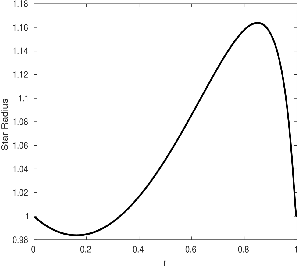
Figure 1: Star Radius as a function of $r$ using the parameters in $Sec\,4.1.1$

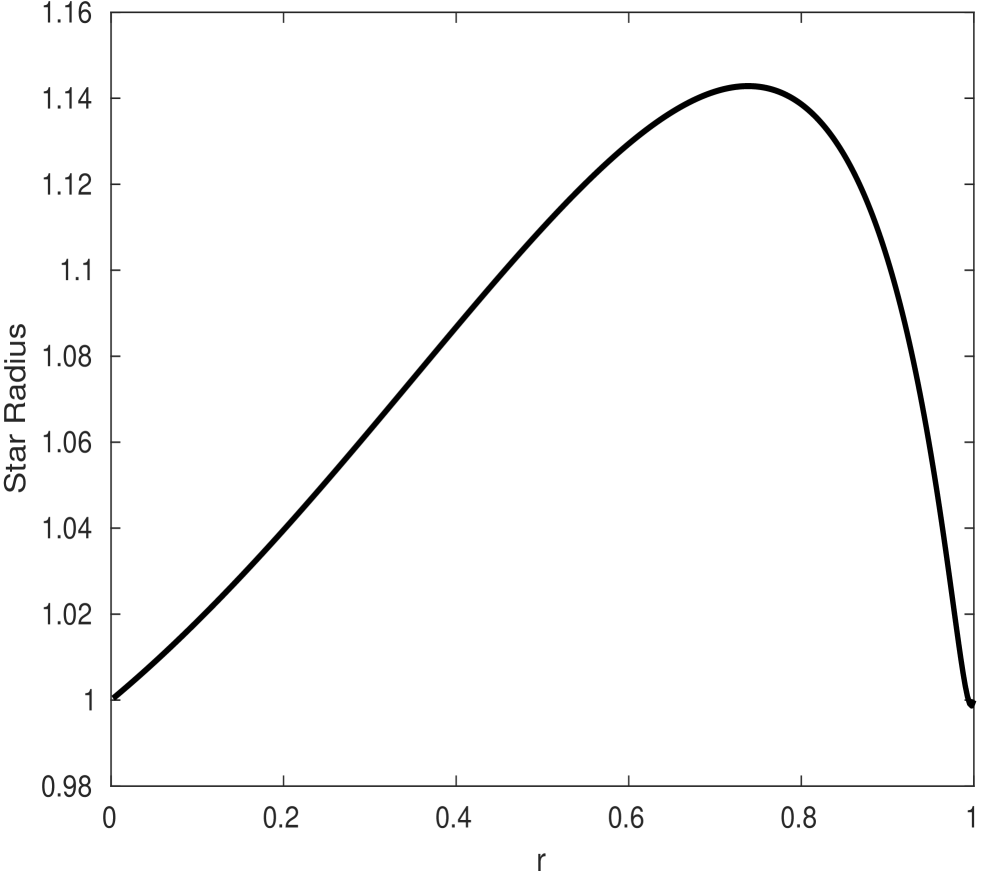
Figure 2: Star Radius as a function of $r$ using the parameters in $Sec\,4.1.3$

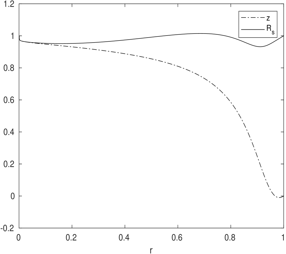
Figure 3: Radius $R_{s}$ and $z$ of a star as a function of $r$

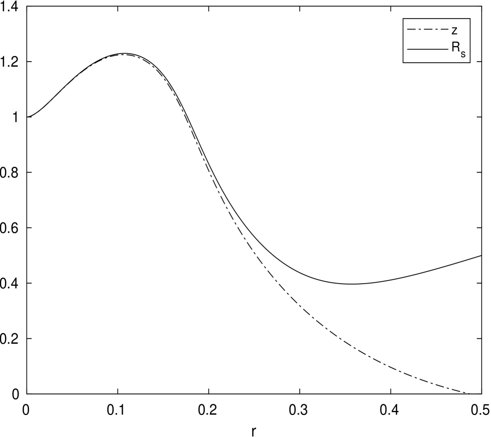
Figure 4: Radius $R_{s}$ and $z$ of a star as a function of $r$, $\lambda=-3.6,\,C=9.658\times 10^{-3}$

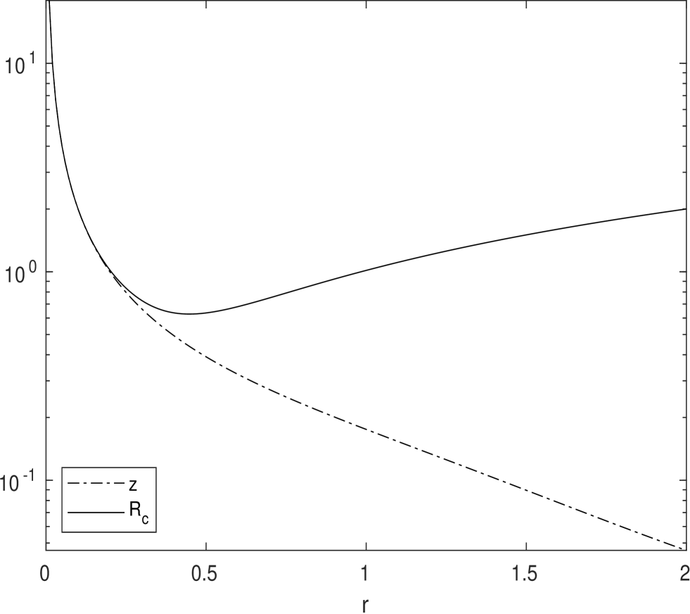
Figure 5: $R_{c}$ and $z$ as a function of $r$ for a cloud with $Z(z)=Az+B$

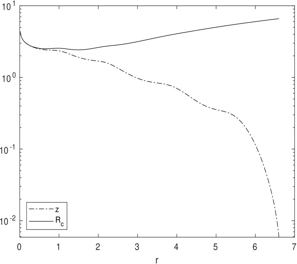
Figure 6: $R_{c}$ and $z$ as a function of $r$ for a cloud with $\lambda=2$

References

- [1] Beskin V. S.: Axisymmetric stationary flows in compact astrophysical objects, Physics-Uspekhi 40 pp. 659-688, 1997.
- [2] Chandrasekhar, S.: An Introduction to the Study of Stellar Structures, University of Chicago Press, Chicago, 1938.
- [3] Chandrasekhar, S: Ellipsoidal figures of equilibrium- an historical account, Comm. Pure Appl. Math, 20 251-265, 1967.
- [4] Friedman, A., Turkington, B.: The oblateness of an axisymmetric rotating fluid, Indiana Univ. Math fluid J., 29 pp.777-792, 1980.
- [5] Humi, M.: Steady States of self gravitating incompressible fluid. J. Math. Phys. 47, 093101 (10 pages), 2006.
- [6] Humi, M.: Steady States of Self Gravitating Incompressible Fluid with Axial Symmetry, Int. J. Mod. Phys. A 24, No. 23 pp. 4287-4303 (2009)
- [7] Humi, M.: A Model for Pattern Formation Under Gravity, Applied Mathematical Modeling 40, pp. 41-49, 2016
- [8] Humi, M :Patterns Formation in a Self-Gravitating Isentropic Gas, Earth Moon Planets Volume 121, Issue 1 (2018) , Pages 1-12, https://doi.org/10.1007/s11038-017-9512-y.
- [9] Humi, M. and Roumas, J :Structure of polytropic stars in General Relativity, Astrophysics and Space Science 364(7)117, 2019 DOI: 10.1007/s10509-019-3608-y
- [10] Humi, M.: On the Evolution of a Primordial Interstellar Gas Cloud, Journal of Mathematical Physics 61, 093504 (2020); https://doi.org/10.1063/1.5144917
- [11] Janga,J and Makino, T: On rotating axisymmetric solutions of the Euler–Poisson equations, Journal of Differential Equations 266, pp. 3942-3972, 2019
- [12] M. Kiguchi M., S. Narita S., Miyama S. M., Hayashi C.: The Equilibria of Rotating Isothermal Clouds, Astrophysical J., 317 pp.830-845, 1987.
- [13] Kovetz, A.: Slowly rotating polytropes. Astrophys. J. 154, pp. 999-1003, 1968.
- [14] Kunzle H.P., Nester J.M.: Hamiltonian formulation of gravitating perfect fluids and the Newtonian limit, J. Math. Phys 25, pp. 1009-1018, 1984.
- [15] Letelier, P.S., Oliveira, S.R.: Exact self-gravitating disks and rings: A solitonic approach ,J. Math. Phys. 28 pp.165-170, 1987.
- [16] Li, Y.Y.: On uniformly rotating stars, Arch. Ration. Mech. Anal, 115 pp.367-393, 1991.
- [17] Luo T and Smoller J.: Existence and Non-linear Stability of Rotating Star Solutions of the Compressible Euler-Poisson Equations, Arch. Ration. Mech. Anal. 191, pp.447-496, 2009.
- [18] Matsumoto, T. and Hanawa T.: Bar and Disk Formation in Gravitationally Collapsing Clouds. Astrophys. J., 521(2), pp.659-670,1999.
- [19] Milne, E.A : The equilibrium of a rotating star. Mon. Not. R. Astron. Soc. 83, pp.118-147, 1923.
- [20] Ortega V. G., Volkov E. and Monte-Lima I.: Axisymmetric instabilities in gravitating disks with mass spectrum, Astronomy and Astrophysics 366, pp.276-280, 2001.
- [21] Paschalidis V., Stergioulas N.: Relativistic Rotating Stars, Living Reviews in Relativity, 20, Article number: 7 (2017) DOI - 10.1007/s41114-017-0008-x
- [22] Prentice, A. J. R., Origin of the Solar system, Earth Moon and Planets, 19, pp. 341-398. (1978)
- [23] Prentice, A.J.R.; Dyt, C.P. . ”A numerical simulation of supersonic turbulent convection relating to the formation of the Solar system”, Monthly Notices of the Royal Astronomical Society. 341 (2): 644–656 (2003).
- [24] Roxburgh I. W., Non-Uniformly Rotating, Self-Gravitating, Compressible Masses with Internal Meridian Circulation, Astrophysics and Space Science, 27,pp.425-435, 1974.
- [25] Tassoul Jean-Louis: Theory of Rotating Stars, Princeton U press, Princeton, NJ. 1978,
- [26] Yih C-S: Stratified flows. Academic Press, New York, NY, 1980.