Fast data-driven model reduction for nonlinear dynamical systems

Abstract

We present a fast method for nonlinear data-driven model reduction of dynamical systems onto their slowest nonresonant spectral submanifolds (SSMs). We use observed data to locate a low-dimensional, attracting slow SSM and compute a maximally sparse approximation to the reduced dynamics on it. The recently released SSMLearn algorithm uses implicit optimization to fit a spectral submanifold to data and reduce the dynamics to the normal form. Here, we present two simplified algorithms, which reformulate manifold fitting and normal form computation as explicit problems under certain assumptions. We show on both numerical and experimental datasets that these algorithms yield accurate and sparse rigorous models for essentially nonlinear (or non-linearizable) dynamics. The new algorithms are significantly simplified and provide a speedup of several orders of magnitude.

I Introduction

Nonlinear dynamical systems are omnipresent in nature and engineering. Examples include beam and plate buckling, Abramian et al. (2020) turbulent fluid flows, Holmes et al. (2012) vibrations in jointed structures, Lacayo et al. (2019) sloshing in fluid tanks, Taylor (1953) and even traffic jams. Orosz and Stépán (2006) As computational resources have grown, so has the interest in data-driven methods, which take input data from experiments or simulations and return a reduced model of the underlying system dynamics. To date, however, no rigorous method has been accepted as a standard for nonlinear system identification and reduced modeling.

Model simplicity (or parsimony) is vital for interpretability, control, and response prediction for mechanical devices. Kutz and Brunton (2022) This has motivated reduction methods based partially or fully on linearization of the underlying dynamics, such as the proper orthogonal decomposition Lumley (1967); Awrejcewicz, Krys’ko, and F. (2004) and the dynamic mode decomposition (DMD). Schmid (2010, 2022) Specifically, DMD obtains the best fit of a linear dynamical system to the data in an equation-free manner, Kutz et al. (2016) often utilizing delay embedding to secure sufficiently many observables. Dylewsky et al. (2022)

Many nonlinear mechanical systems, however, exhibit phenomena that cannot occur in linear systems, such as coexisting isolated steady states, and therefore cannot be captured by linear models. Page and Kerswell (2019) We refer to such phenomena as non-linearizable. Machine learning methods can potentially capture such phenomena, Brunton, Proctor, and Kutz (2016); Lusch, Kutz, and Brunton (2018); Hartman and Mestha (2017); Daniel et al. (2020) but tend to provide models that lack interpretability and perform poorly outside their training range. Loiseau, Brunton, and Noack (2020)

Here, we propose spectral submanifolds (SSMs) to obtain sparse models of nonlinearizable phenomena. An SSM is the smoothest nonlinear continuation of a nonresonant spectral subspace emanating from a steady state, both in autonomous systems and systems with periodic or quasiperiodic forcing. SSMs are unique, attracting, and persistent attracting invariant manifolds in the phase space, that lend themselves well to model reduction. Haller and Ponsioen (2016) Closely linked to SSMs, invariant spectral foliations are the basis of another rigorous approach for extending linear modal analysis to nonlinear systems. Szalai (2020)

An available algorithm Jain et al. (2021) computes spectral submanifolds for mechanical systems defined by differential equations. Ponsioen, Pedergnana, and Haller (2018) This algorithm takes a Taylor expansion of a set of autonomous ODEs and computes the coefficients of an SSM up to any order and dimension. The methodology has been applied to model reduction of systems with hundreds of thousands of degrees of freedom, accurately predicting responses to small harmonic forcing, Ponsioen, Jain, and Haller (2020); Jain, Tiso, and Haller (2018); Jain and Haller (2021) as well as the bifurcations of those responses. Li, Jain, and Haller (2021); Li and Haller (2021)

These developments have motivated applications of SSM theory to locate reduced-order models from data. As a first step, Ref Szalai, Ehrhardt, and Haller, 2017 fitted a multivariate polynomial to the sampling map and computed SSMs on the resulting Taylor expanded dynamics. This yielded good reconstructions of the backbone curves in a clamped-clamped beam experiment. Typically, however, due to the rapid growth in the number of terms, a polynomial expansion of the flow map in the full observable space is sensitive to overfitting and quickly becomes intractable in higher-dimensional systems.

Recently, the numerical method SSMLearn was developed for data-driven SSM identification. Cenedese et al. (2022a) This method alleviates the overfitting of the sampling map by separating the model reduction into two steps: manifold identification and reduced dynamics fitting. Thus, the polynomial fit of the dynamics takes place only on the SSM, and hence the number of terms no longer grows with the data dimensionality. First, the data is embedded in a user-defined observable space. Then a polynomial representation of the SSM is fitted to the data and the data dimensionality is reduced by projection onto the tangent space of the SSM. Using nonlinear optimization techniques, finally a transformation from the reduced coordinates to a normal form is computed, maximizing sparsity while retaining essential nonlinearities. Guckenheimer and Holmes (1983)

While data-driven SSM-based model reduction has been successfully applied to both numerical and experimental data for fluid problems, structural dynamics, and fluid-structure interaction, Cenedese et al. (2022a, b); Kaszás, Cenedese, and Haller (2022) the required implicit optimization can be computationally demanding for high-dimensional systems. This paper introduces two alternative, simplified algorithms that explicitly compute an SSM followed by a normal form transformation on the reduced coordinates. Our key assumption is that the tangent space of the SSM at a fixed point can be found by singular value decomposition (SVD). This enables a major simplification and speedup at the expense of giving up the more general applicability of the previous method.

Our new algorithm, fastSSM, contains an explicit implementation of the cubic normal form for a complex conjugate eigenvalue pair, suited for monomodal oscillatory dynamics on two-dimensional SSMs. Its extension, fastSSM⁺, computes the normal form up to any order and dimensionality. Both algorithms are fully equivalent in the case of cubic normal forms on 2D SSMs.

Our algorithms compute the normal form on SSMs analytically from a numerical fit of the reduced dynamics. This is in contrast to previous methods, which fit the normal form directly to data simultaneously at all required orders. The aims of our new algorithms are accessibility to practitioners, major speedup for rapid prototyping, analysis of higher-dimensional observable spaces, and insight into the differences between numerically and analytically computed normal forms.

The structure of this paper is as follows. The theory is laid out in section II, with a brief introduction to SSMs, a summary of the SSMLearn algorithm, and a detailed description of fastSSM and fastSSM⁺. In section III, we detail how to select an observable space with delay embedding and show how to use SSM-reduced models for forced response prediction. In section IV, we apply the two newly derived algorithms to experiments from a sloshing tank, simulations of a von Krmn beam, and experiments on an internally resonant beam. Finally, in section V we draw conclusions from the examples, suggest additional applications, and outline possible further enhancements to our dynamics-based machine learning model reduction algorithms.

II Model order reduction on spectral submanifolds

We consider nonlinear autonomous dynamical systems of class $\mathcal{C}^{l}$, $l\in\{\mathbb{N}^{+},\ \infty,\ a\}$, with $a$ denoting analyticity, in the form

$$\dot{\bm{y}}=\bm{A}\bm{y}+\bm{f}(\bm{y}),\quad\bm{y}\in\mathbb{R}^{p},\quad\bm{f}\sim\mathcal{O}(|\bm{y}|^{2}),\quad\bm{f}:\mathbb{R}^{p}\to\mathbb{R}^{p}.$$ (1)

We assume $\bm{A}\in\mathbb{R}^{p\times p}$ is diagonalizable and the real parts of its eigenvalues are all non-zero. We denote by $\mathcal{V}_{d}{}$ the slowest $d$-dimensional spectral subspace of $\bm{A}$, i.e., the span of the eigenvectors corresponding to the $d$ eigenvalues with real part closest to zero. When all eigenvalues have negative real parts, the dynamics of the linearized system will converge to $\mathcal{V}_{d}{}$ in forward time.

If the eigenvalues corresponding to $\mathcal{V}_{d}{}$ are non-resonant with the remaining $p-d$ eigenvalues of $\bm{A}$, $\mathcal{V}_{d}$ admits a unique smoothest, invariant, nonlinear continuation $\mathcal{M}$ under addition of the higher-order terms. Cabré, Fontich, and de la Llave (2003) We refer to $\mathcal{M}$ as a spectral submanifold (SSM). Haller and Ponsioen (2016); Cenedese et al. (2022b) In the case of a resonance between $\mathcal{V}_{d}$ and the rest of the spectrum of $\bm{A}$, we can include the resonant modal subspace in $\mathcal{V}_{d}$ and thus obtain a higher-dimensional SSM. If all eigenvalues of $\bm{A}$ have negative real parts, $\mathcal{M}$ will be an attracting slow manifold for system (1), just as $\mathcal{V}_{d}$ is for the linear part of (1).

A numerical package, SSMTool, has been developed for the computation of SSMs from arbitrary finite-dimensional nonlinear systems. Jain et al. (2021); Jain and Haller (2021) More recently, a data-driven algorithm, SSMLearn, has been developed to compute SSMs purely from observables of the dynamical system. Cenedese et al. (2022a, b) In the next section, we first review the SSMLearn algorithm and then discuss two simplified versions of it that enable faster computations under some further assumptions.

II.1 Learning spectral submanifolds from data: SSMLearn

We seek a parametrization of $\mathcal{M}$ from trajectories in an observable space, which may be the full phase space or a suitable embedding, as described in subsection III.1. All our proposed data-driven methods consist of two steps: manifold fitting and normal form computation. While SSMLearn solves these problems with implicit optimization, the other two algorithms we develop here perform all these computations explicitly.

With SSMLearn, Cenedese, Axås, and Haller (2021); Cenedese et al. (2022a) we compute a parametrization of the SSM as a multivariate polynomial

$$\bm{y}(\bm{\xi}) =\bm{M}\bm{\xi}^{1:m}=\bm{V}\bm{\xi}+\bm{M}_{2:m}\bm{\xi}^{2:m},$$ (2)

$$\bm{M} =[\bm{V},\bm{M}_{2},\dots,\bm{M}_{m}],\quad\bm{M}_{i}\in\mathbb{R}^{p\times d_{i}},$$

with the reduced coordinates $\bm{\xi}=\bm{V}^{\top}\bm{y}$ and the tangent space $\bm{V}\in\mathbb{R}^{p\times d}$. Here, $d_{i}$ denotes the number of $d$-variate monomials at order $i$. Throughout this paper, the superscript $(\cdot)^{l:r}$ denotes a vector of all monomials at orders $l$ through $r$. For example, if $\bm{x}=[x_{1},x_{2}]^{\top}$, then

$$\bm{x}^{1:3}=[x_{1},x_{2},x_{1}^{2},x_{1}x_{2},x_{2}^{2},x_{1}^{3},x_{1}^{2}x_{2},x_{1}x_{2}^{2},x_{2}^{3}]^{\top}.$$

Minimization of the distance of the parametrized SSM from the training data points $\bm{y}_{j}$ yields the optimal coefficient matrix $\bm{M}^{\star}\in\mathbb{R}^{p\times d_{1:m}}$, with $d_{1:m}$ denoting the number of $d$-variate monomials from orders 1 up to $m$, as

$$\bm{M}^{\star}=[\bm{V}^{\star},\bm{M}^{\star}_{2:m}] =$$ (3)

$$\mathop{\mathrm{argmin}}_{\bm{V},\bm{M}_{2:m}}\sum_{j} ||\bm{y}_{j}-\bm{V}\bm{V}^{\top}\bm{y}_{j}-\bm{M}_{2:m}(\bm{V}^{\top}\bm{y}_{j})^{2:m}||,$$

subject to the constraints

$$\bm{V}^{\top}\bm{V}=\bm{I},\quad\bm{V}^{\top}\bm{M}_{2:m}=\bm{0}.$$ (4)

Next, we compute the reduced dynamics $\dot{\bm{\xi}}=\bm{R}\bm{\xi}^{1:r}$ on the SSM in polynomial form, with coefficients in the matrix $\bm{R}\in\mathbb{R}^{d\times d_{1:r}}$, by minimizing

$$\mathop{\mathrm{argmin}}_{\bm{R}}\sum_{j}||\dot{\bm{\xi}}_{j}-\bm{R}\bm{\xi}_{j}^{1:r}||.$$ (5)

We now compute the normal form of the reduced dynamics of $\bm{\xi}$ on the SSM. Guckenheimer and Holmes (1983) We seek a nonlinear transformation $\bm{t}^{-1}:\bm{\xi}\mapsto\bm{z}$ to new coordinates $\bm{z}\in\mathbb{C}^{d}$, that reduces the number of coefficients in $\bm{R}$ to a minimum set $\bm{N}\in\mathbb{C}^{d\times d_{1:n}}$. The transformation and normalized dynamics are given by

$$\bm{z} =\bm{t}^{-1}(\bm{\xi})=\bm{H}\bm{\xi}^{1:n}=\bm{W}^{-1}\bm{\xi}+\bm{H}_{2:n}\bm{\xi}^{2:n},$$ (6)

$$\dot{\bm{z}} =\bm{n}(\bm{z})=\bm{N}\bm{z}^{1:n}=\bm{\Lambda}\bm{z}+\bm{N}_{2:n}\bm{z}^{2:n},$$

where $\bm{H}\in\mathbb{C}^{d\times d_{1:n}}$, and $\bm{W}\in\mathbb{C}^{d\times d}$ is the matrix of eigenvectors of the linear part $\bm{R}_{1}=\bm{W}\bm{\Lambda}\bm{W}^{-1}$ of the reduced dynamics. $\bm{N}$ is potentially a very sparse matrix, simplifying the dynamics $\bm{n}(\bm{z})$. The locations of nonzero elements in $\bm{N}$ are determined by any approximate inner resonances between the eigenvalues in $\bm{\Lambda}$. Cenedese et al. (2022a) An example is given in (17).

In SSMLearn, the transformation to the normal form is computed by minimization of the conjugacy error

$$\mathop{\mathrm{argmin}}_{\bm{N},\bm{H}}\sum_{j}||\bm{\nabla}_{\bm{\xi}}\bm{t}^{-1}(\bm{\xi}_{j})\dot{\bm{\xi}}_{j}-\bm{n}(\bm{t}^{-1}(\bm{\xi}_{j}))||.$$ (7)

II.2 Fast SSM identification – fastSSM and fastSSM⁺

To turn the manifold fitting into an explicit problem, we assume that the tangent space of the SSM at the origin can be approximately obtained by singular value decomposition (SVD) on the data. This is typically satisfied sufficiently close to an equilibrium point. Moreover, since data variance prevalently tends to occur along the tangent space of the SSM, SVD is a good candidate for this subspace. A third motivation is that the image of $\mathcal{M}$ in a delay-embedded space tends to be flat, even if $\mathcal{M}$ is strongly curved in the full phase space. Cenedese et al. (2022a) Although the computed manifold may curve significantly, it is not allowed to fold over its tangent space. An overview of the algorithm is shown in Figure 1.

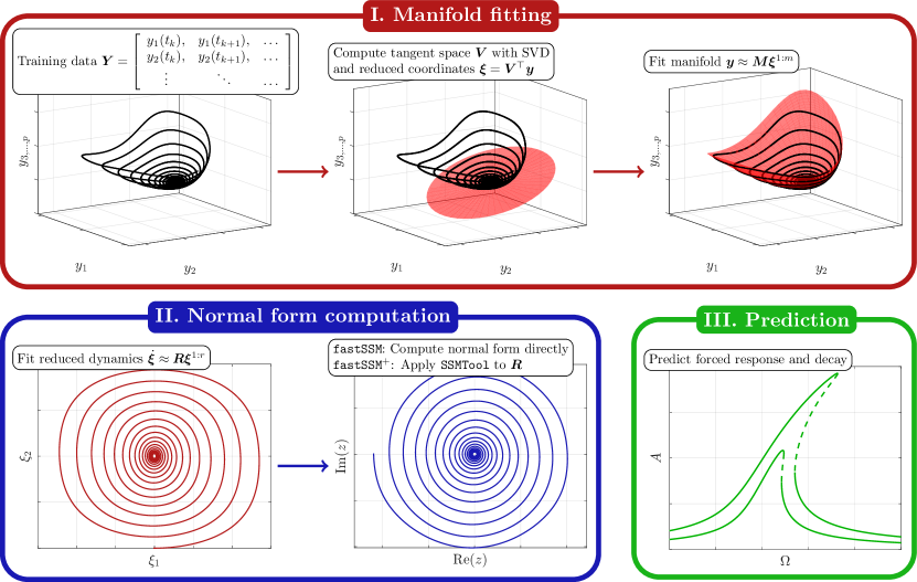
Figure 1: The fastSSM algorithm consists of two main parts, (I) fitting an SSM with SVD and polynomial regression, and (II) computing a normal form on the manifold using SSMTool. The obtained reduced model can then be used for (III) prediction of the autonomous system evolution or the response of the forced system.

The tangent space $\mathcal{V}_{d}{}$ is approximated by $d$-dimensional truncated SVD on the snapshot matrix $\bm{Y}\in\mathbb{R}^{p\times N}$ as

$$\bm{Y}\approx\bm{U}_{d}\bm{S}_{d}\bm{\hat{V}}_{d}^{\top},$$ (8)

where $\bm{U}_{d}\in\mathbb{R}^{p\times d}$, $\bm{S}_{d}\in\mathbb{R}^{d\times d}$, $\bm{\hat{V}}_{d}\in\mathbb{R}^{N\times d}$, and by defining the tangent space approximation as

$$\bm{V}=\bm{U}_{d}\bm{S}_{d}^{-1},$$ (9)

we can project onto it to obtain $d$ reduced coordinates $\bm{\xi}$ as

$$\bm{\xi}=\bm{V}^{\top}\bm{y}.$$ (10)

We denote by $\bm{\Xi}\in\mathbb{R}^{d\times N}$ the projection of $\bm{Y}$ onto $\bm{V}$. Numerically, it is beneficial to first normalize each column of $\bm{V}$ with the maximum absolute value of the corresponding row in $\bm{\hat{V}}_{d}$

The manifold parametrization coefficients $\bm{M}\in\mathbb{R}^{p\times d_{1:m}}$ are obtained by polynomial regression:

$$\bm{y}\approx\bm{M}\bm{\xi}^{1:m},\quad\bm{M}=\bm{Y}(\bm{\Xi}^{1:m})^{\dagger},$$ (11)

with $(\cdot)^{\dagger}$ denoting the Moore-Penrose pseudo-inverse.

The reduced dynamics are approximated by an $\mathcal{O}(r)$ polynomial regression, with the coefficient matrix $\bm{R}\in\mathbb{R}^{d\times d_{1:r}}$, as

$$\dot{\bm{\xi}}\approx\bm{R}\bm{\xi}^{1:r},\quad\bm{R}=\dot{\bm{\Xi}}(\bm{\Xi}^{1:r})^{\dagger}.$$ (12)

The time derivative $\dot{\bm{\xi}}$ may be computed numerically. The quality of this approximation is important for model accuracy. Therefore, we use a central finite difference method including 4 adjacent points in each time direction. Fornberg (1988)

Next, diagonalizing the linear part $\bm{R}_{1}=\bm{W}\bm{\Lambda}\bm{W}^{-1}$, we again apply regression to rewrite $\bm{R}$ in the form $\bm{G}\in\mathbb{C}^{d\times d_{1:r}}$ with the eigenvalues in the linear part $\bm{G}_{1}=\bm{\Lambda}$ and modal coordinates $\bm{\zeta}=\bm{W}^{-1}\bm{z}$, such that

$$\dot{\bm{\zeta}}\approx\bm{G}\bm{\zeta}^{1:r}.$$ (13)

To compute the normal form of (13), we seek a near-identity polynomial transformation $\bm{t}:\bm{z}\mapsto\bm{\zeta}$ with coefficients $\bm{T}\in\mathbb{C}^{d\times d_{1:n}}$ from new coordinates $\bm{z}\in\mathbb{C}^{d}$ such that

$$\bm{\zeta} =\bm{t}(\bm{z})=\bm{T}\bm{z}^{1:n}=\bm{z}+\bm{T}_{2:n}\bm{z}^{2:n}$$ (14)

$$\dot{\bm{z}} =\bm{n}(\bm{z})=\bm{N}\bm{z}^{1:n}=\bm{\Lambda}\bm{z}+\bm{N}_{2:n}\bm{z}^{2:n}.$$

We enforce conjugacy between the normal form and reduced dynamics by plugging (14) into (13):

$$\bm{\nabla}_{\bm{z}}(\bm{T}\bm{z}^{1:n})\bm{N}\bm{z}^{1:n}=\bm{G}(\bm{T}\bm{z}^{1:n})^{1:r}.$$ (15)

We can compute $\bm{T}$ and $\bm{N}$ by solving (15) recursively at increasing orders. See Ref. Jain and Haller, 2021 for details on the computations.

The simplest non-trivial normal form arises on a 2D manifold emanating from a spectral subspace corresponding to two complex conjugate eigenvalues $(\lambda,\bar{\lambda})$ with small real part. We denote the coordinates in the normal form $(z_{1},z_{2})=(z,\bar{z})$. The cubic normal form, with $\gamma\in\mathbb{C}$, is

$$\dot{z} =\lambda z+\gamma z^{2}\bar{z}+\mathcal{O}(5)$$ (16)

$$\dot{\bar{z}} =\bar{\lambda}\bar{z}+\bar{\gamma}z\bar{z}^{2}+\mathcal{O}(5),$$

for which we obtain

$$\bm{N}=\left[\begin{array}[]{ccccccccc}\lambda&0&0&0&0&0&\gamma&0&0\\ 0&\bar{\lambda}&0&0&0&0&0&\bar{\gamma}&0\end{array}\right].$$ (17)

Solving (15) yields

$$\bm{T}=\left[\begin{array}[]{ccccccccc}1&0&T_{3}&T_{4}&T_{5}&T_{6}&0&T_{8}&T_{9}\\ 0&1&\bar{T}_{5}&\bar{T}_{4}&\bar{T}_{3}&\bar{T}_{9}&\bar{T}_{8}&0&\bar{T}_{6}\end{array}\right],$$ (18)

where

$$T_{3} =\frac{G_{3}}{\lambda},\quad T_{4}=\frac{G_{4}}{\bar{\lambda}},\quad T_{5}=\frac{G_{5}}{2\bar{\lambda}-\lambda},$$ (19)

$$T_{6} =\frac{2G_{3}T_{3}+G_{4}\bar{T}_{5}+G_{6}}{2\lambda},\quad T_{9}=\frac{G_{4}T_{5}+2G_{5}\bar{T}_{3}+G_{9}}{3\bar{\lambda}-\lambda},$$

$$T_{8} =\frac{2G_{3}T_{5}+G_{4}\bar{T}_{3}+G_{4}T_{4}+2G_{5}\bar{T}_{4}+G_{8}}{2\bar{\lambda}},$$

$$\gamma =2G_{3}T_{4}+G_{4}\bar{T}_{4}+G_{4}T_{3}+2G_{5}\bar{T}_{5}+G_{7},$$

and $G_{i}$ refers to element $i$ of the top row in $\bm{G}$. Szalai, Ehrhardt, and Haller (2017)

This solution is implemented in fastSSM for fast, cubic-order, 2D normal form computations. We have the reduced dynamics and normal form orders $r=3$ and $n=3$, and we are free to set the order $m$ of the manifold.

While a cubic order normal form will suffice to model a number of datasets accurately, Cenedese et al. (2022a, b) for stronger nonlinearities we must include higher orders. SSMTool can solve (15) for any dimension and order of expansion. The algorithm fastSSM⁺ extends the manifold fitting and normal form computation in fastSSM to any dimension and order by automatically applying SSMTool to the coefficients of $\bm{R}$. In principle, we are free to choose any orders $m$, $r$, and $n$, but to avoid overfitting we must limit the manifold order $m$ and reduced dynamics order $r$. In addition, we need to pick a large enough $n$ to make the tail of the SSM-reduced dynamics small enough.

Unlike (3) and (7) in SSMLearn, all computations in fastSSM and fastSSM⁺ are explicit. Therefore, we expect these algorithms to be faster than SSMLearn, at the cost of some model accuracy. Further, we note that in fastSSM and fastSSM⁺, the normal form is computed analytically from a numerical polynomial fit, whereas SSMLearn directly fits the normal form coefficients numerically from data.

In practice we must also approximate the inverse of $\bm{t}$ to transform initial conditions to the normal form before the integration. The most accurate and simplest way is a numerical solution for each initial condition, but a general inverse map can also be computed. Accordingly, in fastSSM, we implement explicitly the 3rd-order polynomial expansion of the inverse of $\bm{t}$, whereas fastSSM⁺ fits a polynomial map by regression on the training data.

Finally, we note that all our methods require that the data lies sufficiently close to an invariant manifold. We achieve this by removing any initial transients from the training dataset, as identified by a spectral analysis on the input signal. Cenedese et al. (2022b) Since the SSM is unique and attracting, this procedure ensures that we train on relevant data.

III Pre- and post-processing of the data

We present here considerations for the delay embedding of observable functions to facilitate manifold identification. We also show how to use the obtained normal form dynamics to predict the forced response of the full system.

III.1 Embedding spectral submanifolds in the observable space

In practice, observing trajectories $\bm{x}(t)$ in the full phase space is often intractable. For instance, an experimentalist might only observe a scalar quantity $s(t)=\zeta(\bm{x}(t))$. Nevertheless, if the observable function $\zeta:\mathbb{R}^{n_{\mathrm{full}}}\to\mathbb{R}$ is generic, it can be used to reconstruct an invariant manifold of the system in an observable space via delay embedding.

To this end, we collect $p$ measurements separated by a time lag $\tau>0$ to form a vector $\bm{y}$ in an observable space $\mathbb{R}^{p}$ as

$$\bm{y}(t)=[s(t),s(t+\tau),s(t+2\tau),\dots,s(t+(p-1)\tau)]^{\top}.$$

Takens’ embedding theorem implies that if $\bm{x}(t)$ lies on an invariant $d$-dimensional manifold $\mathcal{M}$ in the original phase space, then $\bm{y}(t)$ lies on a diffeomorphic copy of $\mathcal{M}$ in $\mathbb{R}^{p}$ with probability one, if $p\geq 2d+1$ and $\zeta(\bm{x})$ is a generic observable. Takens (1981) This result also extends to generic multivariate functions $\bm{\zeta}:\mathbb{R}^{n_{\mathrm{full}}}\to\mathbb{R}^{n_{\mathrm{obs}}}$ as long as the total observable space dimension exceeds $2d$. Sauer, Yorke, and Casdagli (1991); Deyle and Sugihara (2011) Even with a high-dimensional observable, however, we apply delay embedding to diversify the data and unveil information about the time derivative of the signal in our later sloshing example. Cenedese et al. (2022b)

The timelag $\tau$ is typically a multiple of the sampling time or timestep $\Delta t$ of the available dataset. The default choice is $\tau=\Delta t$, but one can also increase the time lag to $\tau=k\Delta t$, $k\in\mathbb{N}_{+}$. Delay-embedding an observed time series $[s(t_{1}),\dots,s(t_{N})]$ thus yields the snapshot matrix

$$\bm{Y}=\left[\begin{array}[]{cccc}s(t_{1})&s(t_{2})&\dots&s(t_{N+(1-p)k})\\ s(t_{k+1})&s(t_{k+2})&\dots&s(t_{N+(2-p)k})\\ s(t_{2k+1})&s(t_{2k+2})&\dots&s(t_{N+(3-p)k})\\ \vdots&\vdots&\ddots&\vdots\\ s(t_{(p-1)k+1})&s(t_{(p-1)k+2})&\dots&s(t_{N})\end{array}\right].$$ (20)

Takens’ embedding theorem requires at least $k=1$, $p=2d+1$, which typically suffices for SSM identification when $d=2$.

If we observe a smooth scalar signal $s(t)$, then for small $\tau$, we have

$$s(t+j\tau)=s(t)+\dot{s}(t)j\tau+\mathcal{O}((j\tau)^{2}).$$

Delay-embedding $s(t)$ then yields

$$\bm{y}(t)=\left[\begin{array}[]{c}s(t)\\ s(t+\tau)\\ s(t+2\tau)\\ \vdots\\ s(t+(p-1)\tau)\end{array}\right]=s(t)\left[\begin{array}[]{c}1\\ 1\\ 1\\ \vdots\\ 1\end{array}\right] +\dot{s}(t)\tau\left[\begin{array}[]{c}0\\ 1\\ 2\\ \vdots\\ p-1\end{array}\right]$$ (21)

$$+\mathcal{O}((p\tau)^{2}).$$

As noted in Ref. Cenedese et al., 2022a, if $\tau$ and $p$ are small in comparison to $\dot{s}$, then the diffeomorphic copy of $\mathcal{M}$ in the observable space is approximately a plane spanned by the two constant vectors appearing in (21).

For multimodal signals, however, $p$ and $k$ must be increased to allow distinction between the modes in the observable space. The modal subspaces of the full phase space have corresponding planes in the observable space, which must be identified to provide reduced coordinates for the SSM. A low delay embedding dimension and an overly short timelag can make these planes close to parallel, which complicates their identification. In contrast, we want to pick the timelag and embedding dimension such that the images of the modal subspaces in the observable space are close to orthogonal.

To illustrate this, we consider an observed superposition of two harmonics $s(t)=a\cos(\omega_{1}t+\psi_{1})+b\cos(\omega_{2}t+\psi_{2})$, a reasonable model of a typical signal close to the origin. Using a trigonometric identity, we can rewrite

$$s(t+j\tau) =a\cos(\omega_{1}t+\psi_{1})\cos(\omega_{1}j\tau)-$$ (22)

$$a\sin(\omega_{1}t+\psi_{1})\sin(\omega_{1}j\tau)+$$

$$b\cos(\omega_{2}t+\psi_{2})\cos(\omega_{2}j\tau)-$$

$$b\sin(\omega_{2}t+\psi_{2})\sin(\omega_{2}j\tau).$$

The delay-embedded observable vector is therefore

$$\bm{y}(t)=\left[\begin{array}[]{c}s(t)\\ s(t+\tau)\\ s(t+2\tau)\\ \vdots\\ s(t+(p-1)\tau)\end{array}\right]=\bm{V}\left[\begin{array}[]{c}a\cos(\omega_{1}t+\psi_{1})\\ -a\sin(\omega_{1}t+\psi_{1})\\ b\cos(\omega_{2}t+\psi_{2})\\ -b\sin(\omega_{2}t+\psi_{2})\end{array}\right],$$ (23)

where

$$\bm{V}^{\top}=\left[\begin{array}[]{ccccc}1&\cos(\omega_{1}\tau)&\cos(2\omega_{1}\tau)&\dots&\cos((p-1)\omega_{1}\tau)\\ 0&\sin(\omega_{1}\tau)&\sin(2\omega_{1}\tau)&\dots&\sin((p-1)\omega_{1}\tau)\\ 1&\cos(\omega_{2}\tau)&\cos(2\omega_{2}\tau)&\dots&\cos((p-1)\omega_{2}\tau)\\ 0&\sin(\omega_{2}\tau)&\sin(2\omega_{2}\tau)&\dots&\sin((p-1)\omega_{2}\tau)\\ \end{array}\right].$$ (24)

The trajectories will reside on a 4-dimensional hyperplane given by the constant matrix $\bm{V}$ of delay-embedded harmonic functions. Picking $\tau$ and $p$ too small complicates manifold identification, because the columns of $\bm{V}$ are close to linearly dependent. Instead, we choose a timelag such that these planes are as close to orthogonal as possible. Based on these considerations, we select a timelag $\tau=k\Delta t$ such that $\omega_{2}\tau\approx\frac{\pi}{2}$, where $\omega_{2}$ is the second eigenfrequency of the observed system. This argument generalizes to any number of modes, although the choice of $k$ becomes more complicated. The embedding dimension $p$ is set to at least $2d+1$. Further increases to $p$ can facilitate identification of a manifold but also complicate its geometry far from the origin.

III.2 Backbone curves and forced response

If all eigenvalues of the reduced dynamics are complex conjugate pairs, we can rewrite the normal form on the SSM in polar coordinates $(\bm{\rho},\bm{\theta})$ with $z_{\ell}=\rho_{\ell}\mathrm{e}^{i\theta_{\ell}}$, $z_{\ell+1}=\rho_{\ell}\mathrm{e}^{-i\theta_{\ell}}$. This yields the SSM-reduced dynamics in the form

$$\dot{\rho}_{\ell} =c_{\ell}(\bm{\rho},\bm{\theta})\rho_{\ell},$$ (25)

$$\dot{\theta}_{\ell} =\omega_{\ell}(\bm{\rho},\bm{\theta}).$$

If the imaginary parts of all eigenvalue pairs are non-resonant with each other, then the functions $c_{\ell}$ and $\omega_{\ell}$ depend only on $\bm{\rho}$. Ponsioen, Pedergnana, and Haller (2018) For example, the cubic 2D normal form (16) in polar coordinates reads

$$\dot{\rho} =\mathrm{Re\,}(\lambda)\rho+\mathrm{Re\,}(\gamma)\rho^{3}+\mathcal{O}(\rho^{5}),$$ (26)

$$\dot{\theta} =\mathrm{Im\,}(\lambda)+\mathrm{Im\,}(\gamma)\rho^{2}+\mathcal{O}(\rho^{4}).$$

For the general 2D case, we define an amplitude as

$$\mathcal{A}(\rho)=\max_{\theta\in[0,2\pi)}\left|\alpha\left(\bm{W}\bm{t}\left(\left[\begin{array}[]{c}\rho\mathrm{e}^{i\theta}\\ \rho\mathrm{e}^{-i\theta}\end{array}\right]\right)\right)\right|,$$ (27)

where $\alpha:\mathbb{R}^{p}\to\mathbb{R}$ is a function mapping from the observable space to some amplitude of a particular degree of freedom or the norm of total displacements. The backbone curve of that amplitude is then defined as the parametrized curve

$$\mathcal{B}(\rho)=(\omega(\rho),\mathcal{A}(\rho)),$$ (28)

which is broadly used in the field of nonlinear vibrations to illustrate the overall effect of nonlinearities in the system.

Next, following Refs. Breunung and Haller, 2018; Ponsioen, Pedergnana, and Haller, 2019, we use the data-driven normal form on the SSM to predict the response of the system under additional, time-periodic external forcing. This amounts to adding a forcing term with amplitude $f$ and frequency $\Omega$ to the general 2D normal form to obtain

$$\dot{\rho} =c(\rho)\rho+f\sin\psi,$$ (29)

$$\dot{\psi} =\omega(\rho)-\Omega+\frac{f}{\rho}\cos\psi,$$

where we have introduced the phase difference $\psi=\theta-\Omega t$. The forced response curve (FRC) is then defined as the bifurcation curve of the fixed points $(\rho_{0},\psi_{0})$ of (29) under varying $\Omega$. Squaring and adding the equations in (29) yields a parametrization of the FRC for the forcing frequency $\Omega$ and the phase lag $\psi_{0}$ in the form

$$\Omega(\rho_{0},f) =\omega(\rho_{0})\pm\sqrt{\frac{f^{2}}{\rho_{0}^{2}}-(c(\rho_{0}))^{2}},$$ (30)

$$\psi_{0}(\rho_{0},f) =-\arcsin\left(\frac{c(\rho_{0})\rho_{0}}{f}\right).$$

Since the relation between the experimental forcing and the normal form forcing $f$ is unknown, a calibration of each FRC to at least one observation of a forced response is necessary. Following Refs. Cenedese et al., 2022a, b, we achieve this by prescribing a single intersection point on the FRC in the frequency-amplitude plane. We use the calibration frequency $\Omega_{\mathrm{cal}}$ and amplitude $u_{\mathrm{cal}}$ of the maximal experimental response at each forcing level. The mapping to an equivalent point $\bm{y}_{\mathrm{cal}}$ in the observable space can then be approximated by delay-embedding a cosine signal of amplitude $u_{\mathrm{cal}}$ and frequency $\Omega_{\mathrm{cal}}$. We compute the calibration amplitude $\rho_{\mathrm{cal}}$ by projecting $\bm{y}_{\mathrm{cal}}$ onto the manifold and transforming to the normal form. The forcing $f$ is then computed from the relationship

$$f^{2}=(c(\rho_{\mathrm{cal}}))^{2}\rho_{\mathrm{cal}}^{2}+(\omega(\rho_{\mathrm{cal}})-\Omega)^{2}\rho_{\mathrm{cal}}^{2}.$$ (31)

Finally, under periodic forcing, the SSM parametrization becomes time-dependent with the addition of a small periodic term. We ignore this contribution here to simplify the analysis, but note that this small non-autonomous correction can be exactly computed using SSMLearn. Cenedese et al. (2022a, b)

IV Examples

We now apply fastSSM and fastSSM⁺ to three datasets: sloshing experiments in a water tank, simulation of a clamped-clamped von Krmn beam, and experiments on an internally resonant beam.

We quantify the quality of our SSM-reduced models with the normalized mean trajectory error (NMTE). Cenedese et al. (2022a) Given a test trajectory with $N$ snapshots $\bm{y}(t_{j})$ and the model-based reconstruction $\hat{\bm{y}}(t_{j})$ obtained by integrating the normal form dynamics and mapping back to the observable space, the NMTE is defined as

$$\mathrm{NMTE}=\frac{1}{N\max_{j}||\bm{y}(t_{j})||}\sum_{j=1}^{N}||\hat{\bm{y}}(t_{j})-\bm{y}(t_{j})||.$$ (32)

IV.1 Tank sloshing

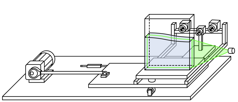
Figure 2: Sloshing experiment setup with the partially filled tank and the cameras, mounted on a platform excited by a motor.

A tank partially filled with a liquid responds nonlinearly to horizontal harmonic excitation. Taylor (1953) Stronger fluid oscillation gives rise to more shearing against the tank wall, so that the damping of the system increases nonlinearly with the amplitude. Faltinsen and Timokha (2009) In addition, the instantaneous frequency decreases at higher amplitudes. Both phenomena are crucial for predicting the forced response amplitude of the liquid. The industrial applications for sloshing models are numerous, ranging from the transportation of fluids in trucks Cheli et al. (2013) and container ships Faltinsen and Timokha (2009) to the design of fuel tanks for spacecraft. Dodge (2000); Abramson (1966)

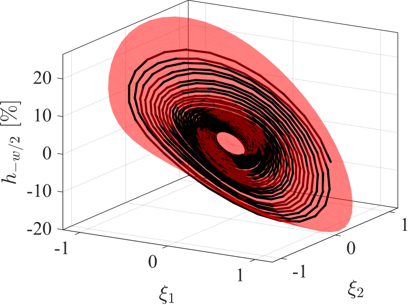
(a)

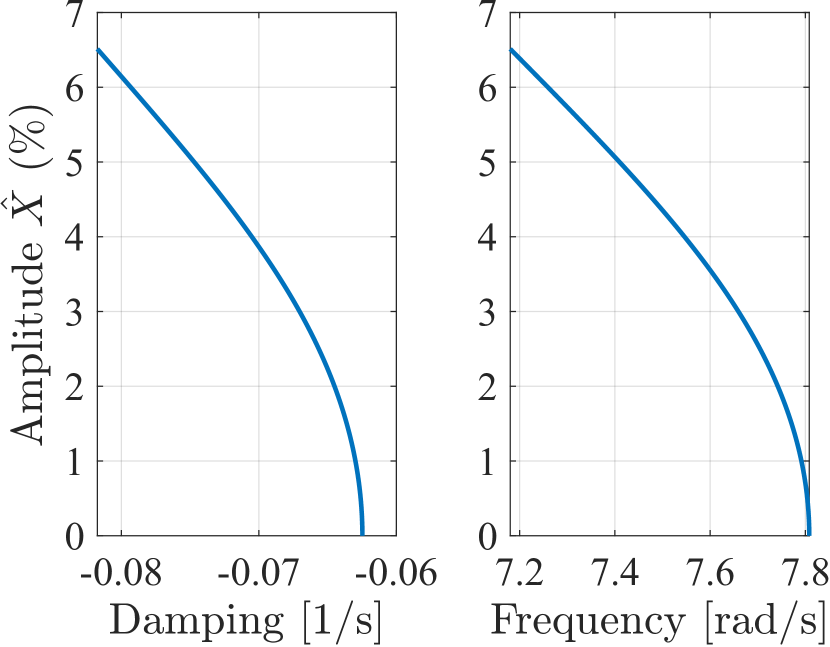
(b)

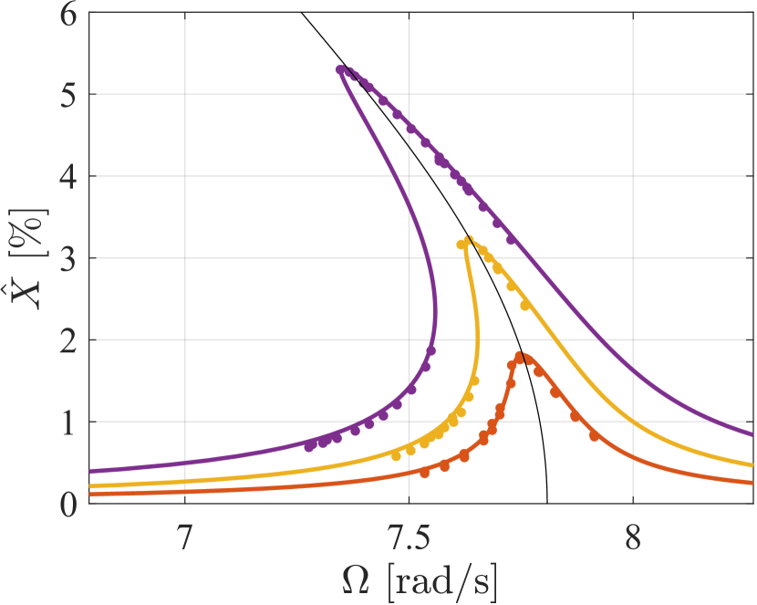
(c)

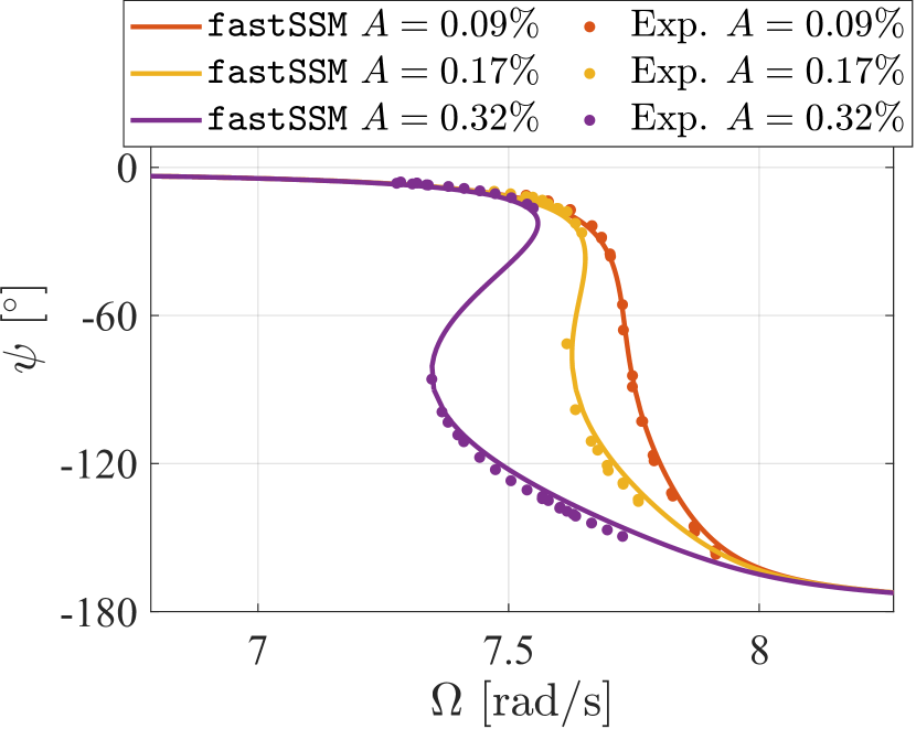
(d)

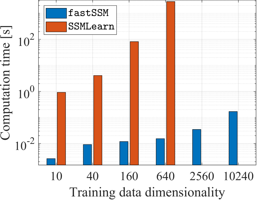
(e)

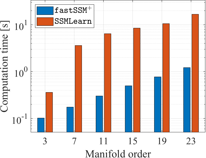
(f)

Figure 3: (3(a)) A visualization of the identified 2D SSM, with the wall surface amplitude on the vertical axis. (3(b)) The computed instantaneous damping and frequency show significant nonlinearity. (3(c)) Prediction of the forced response amplitude and (3(d)) phase lag compared with experimental results for three different forcing amplitudes. (3(e)) The computational cost of manifold fitting is orders of magnitude lower with fastSSM than with SSMLearn, and scales better with higher dimensionality. (3(f)) fastSSM⁺ normal form computation is also faster, although SSMLearn tends to require a lower order for convergence.

In Ref. Cenedese et al., 2022a, SSMLearn was applied to experimental sloshing data from Ref. Bäuerlein and Avila, 2021. With nonlinear models of both frequency and damping, the forced response of the first oscillation mode was accurately predicted from unforced decaying center of mass signals. Here, we will apply fastSSM to a much higher-dimensional observable space that includes fine-resolved surface profile data.

The experiments described in Ref. Bäuerlein and Avila, 2021 were performed in a rectangular tank of width $w=500$ mm and depth $l=50$ mm, partially filled with water up to a height of 400 mm. The tank was mounted on a moving platform excited harmonically by a motor at different frequencies $\Omega$ and amplitudes $A$. A camera was mounted on the moving platform, and the surface profile $\bm{h}$ was detected via image processing with the sampling time $\Delta t=0.033$ s. Figure 2 displays the experimental setup.

From the surface profile, the sloshing amplitude can be quantified by computing the horizontal position $\hat{X}$ of the liquid’s center of mass at each time, normalized by the tank width. $\hat{X}$ is a physically meaningful quantity, relevant for engineering applications and robust against small image evaluation errors. The tank was excited at the tested frequencies until a steady state was reached, and the driving was turned off. The oscillation amplitude then decayed along the backbone curve defined in (28).

Here we append the $\hat{X}$ signal with the measurements of the surface elevation $\bm{h}$ at $1\,531$ points. We delay-embed these signals using 10 subsequent measurements to create a $15\,320$-dimensional observable space, in which fastSSM identifies a 2-dimensional, 7th-order manifold, shown in 3(a). We identify the reduced dynamics on the SSM up to 3rd order, and then compute its 3rd-order normal form

$$\dot{\rho} =-0.062\rho-0.019\rho^{3},$$ (33)

$$\rho\dot{\theta} =7.81\rho-0.628\rho^{3}.$$

The backbone curves obtained from this normal form are shown in 3(b).

In Figures 3(c) and 3(d), we compute forced response curves for the center of mass position, $\hat{X}$, and compare to its experimentally generated values obtained along frequency sweeps from both directions. We find the response prediction from fastSSM to be accurate. In particular, the nonlinear damping term of the normal form helps capturing the width of the forced response curve at higher amplitudes.

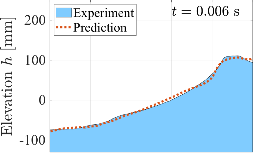
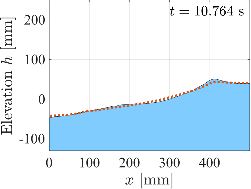
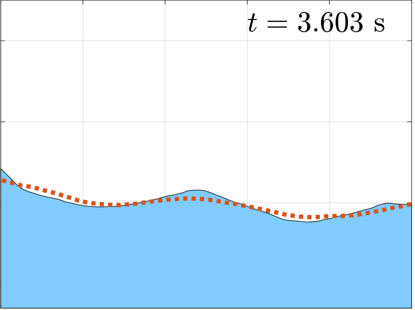
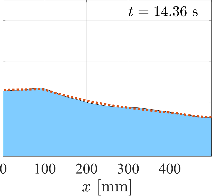
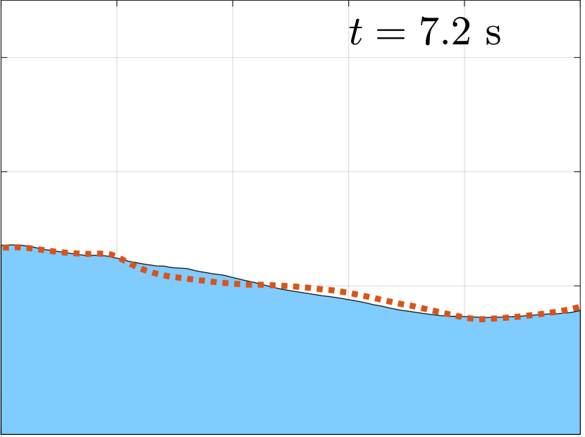
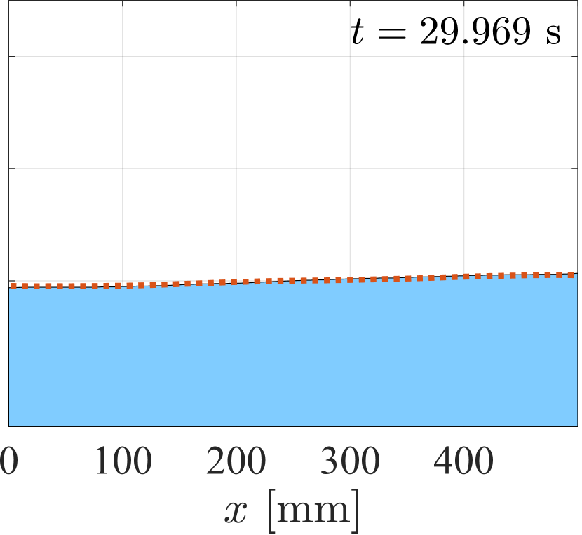
Figure 4: Snapshots of the fastSSM prediction of the surface profile decay. The initial condition is transformed to the SSM-reduced system, which is integrated to produce a 2D trajectory in normal form coordinates. By mapping the trajectory back to the observable space, we can predict the full surface profile and observe close agreement with the experiments in phase, amplitude, and shape.

We also use the normal form (33) to predict the development of the decaying full surface profile $\bm{h}$ in Figure 4. Here, we take the initial surface profile and transform it to an initial condition in the normal form coordinates. We integrate the normal form from this initial condition to predict its development in the observable space. We observe that the prediction is in close agreement with experiments, yielding a total NMTE of 2.05 % over the entire phase space.

Finally, we compare execution times for fastSSM and SSMLearn when they are trained on the surface profile data. These computations were performed on MATLAB version 2020b, installed on an iMac with 2.3 GHz 18-Core Intel Xeon W and 128 GB RAM.

In 3(e), the computational effort of fitting a 2D SSM is plotted against the dimensionality of the training data, i.e., the number of included surface points multiplied by the delay embedding dimension 10. Due to its explicit coefficient fitting, fastSSM achieves a major speedup, and enables analysis of significantly higher-dimensional data than SSMLearn.

After reduction to the manifold, both SSMLearn and fastSSM compute the $\mathcal{O}(3)$ normal form in less than a second. In order to compare the computational effort for higher order normal forms, we apply fastSSM⁺. 3(f) shows the time required to compute a 2D normal form after fitting the SSM to the sloshing data. At a given order, fastSSM⁺ is on average 15 times faster than SSMLearn. While both methods are fast in this example, the difference becomes significant at higher dimensions. It should be noted, however, that in strongly nonlinear cases, fastSSM⁺ may require a higher order normal form to converge, and so the difference to the practitioner may be smaller. This difference in the convergence of normal forms is closer examined in the next example.

IV.2 von Krmn beam

(a)

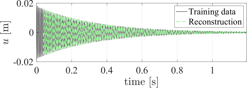
(b)

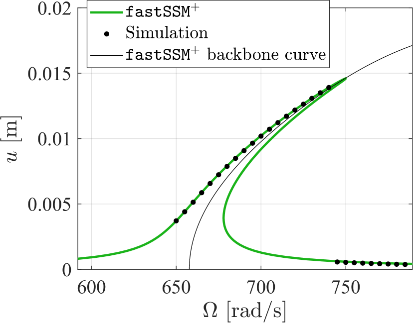
(c)

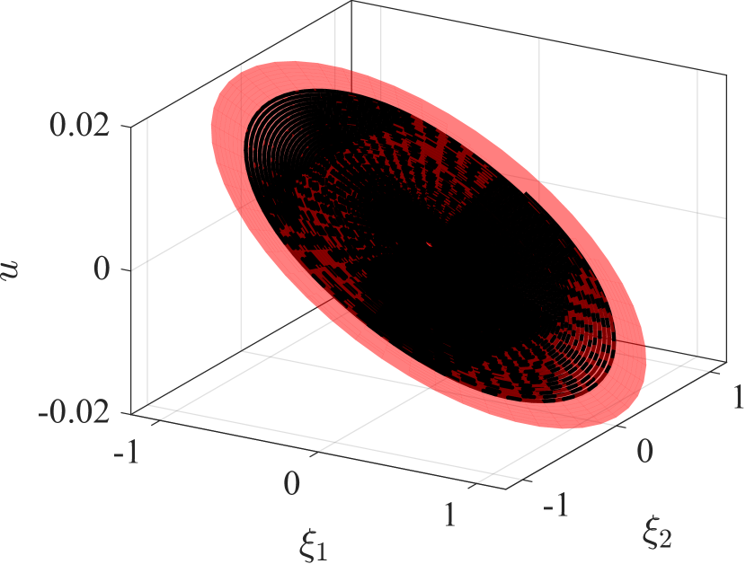
(d)

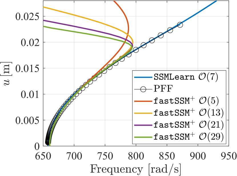
(e)

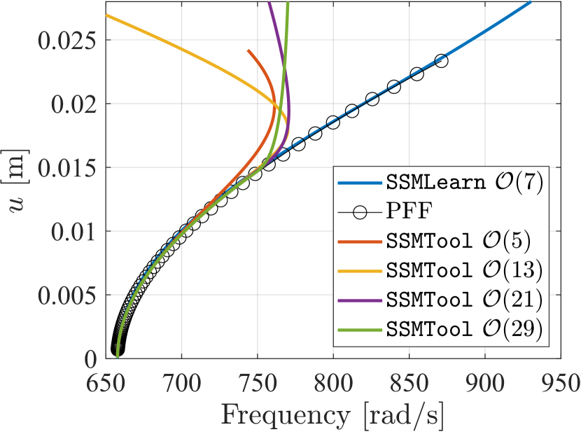
(f)

Figure 5: (5(a)) The observable is the midpoint displacement $u(t)$ of a 12-element von Krmn clamped-clamped beam. (5(b)) Based on an $\mathcal{O}(5)$ reduced dynamics model, fastSSM⁺ returns a normal form that predicts the displacement decay accurately. (5(c)) Prediction of the forced response amplitude. (5(d)) The 2D SSM visualized in a 3D representation of the observable space. Above 20 mm deflection, increased orders of fastSSM⁺ (5(e)) and SSMTool (5(f)) no longer improve the backbone curve approximation. Higher amplitudes lie beyond the radius of convergence of the SSM Taylor expansion. SSMLearn, however, continues to approximate the backbone curve well beyond this limit.

We consider data from numerical simulations of a finite-element model of a clamped-clamped von Krmn nonlinear beam. Jain, Tiso, and Haller (2018) Each element has three degrees of freedom: axial deformation $u_{0}$, transverse deflection $w_{0}$, and rotation $w_{0}^{\prime}$. The nonlinear von Krmn axial strain approximation is

$$\epsilon_{11}=u_{0}^{\prime}(x_{1})+\frac{1}{2}\left(w_{0}^{\prime}(x_{1})\right)^{2}-zw_{0}^{\prime\prime}(x_{1}),$$ (34)

where the second term sets this model apart from the linear Euler-Bernoulli beam. The axial stress is modeled as

$$\sigma=E\epsilon_{11}+\kappa\dot{\epsilon}_{11},$$ (35)

where $E$ is the Young’s modulus and $\kappa$ is the material rate of viscous damping.

After a convergence analysis, we set the number of elements to 12, which results in a 33-degree of freedom mechanical system, i.e., a 66-dimensional phase space. As initial condition, we compute the response to a static transverse load of 14 kN at the midpoint, removed at the simulation start. Our observable function is the midpoint displacement, and the objective is to reconstruct the SSM and its dynamics in the observable space by delay-embedding the signal. A sketch of the system is shown in 5(a).

We set $E=70$ GPa, $\kappa=1.0\times 10^{6}$ $\mathrm{Pa\cdot s}$, length 1000 mm, width 50 mm, and thickness 20 mm. The sampling time is $\Delta t=0.0955$ s. To satisfy the conditions of Takens’ embedding theorem, we set the delay embedding dimension to $p=5$. The maximum displacement in the training data is 15.9 mm.

The cubic normal form in fastSSM is insufficient to describe the higher amplitude oscillations, so we deploy fastSSM⁺ to compute a higher-order normal form. After training on the generated trajectory, fastSSM⁺ outputs a normal form that we use for forced response prediction. We use a 1st-order SSM, 5th-order SSM-reduced dynamics, and obtain an 11th-order normal form

$$\dot{\rho} =-3.12\rho-0.899\rho^{3}+4.12\rho^{5}-$$ (36a)

$$12.4\rho^{7}+16.0\rho^{9}-17.7\rho^{11},$$

$$\rho\dot{\theta} =658\rho+263\rho^{3}-155\rho^{5}+$$ (36b)

$$151\rho^{7}-181\rho^{9}+237\rho^{11},$$

which yields a NMTE of 0.63 % on the training data (5(b)).

We compute the FRC and verify it against a numerical integration frequency sweep in 5(c). Clearly, the autonomous SSM computed by fastSSM⁺ can predict the forced response very accurately even with strong nonlinearities. 5(d) shows a representation of the SSM geometry, which, as predicted in subsection III.1, is almost flat due to the small timelag.

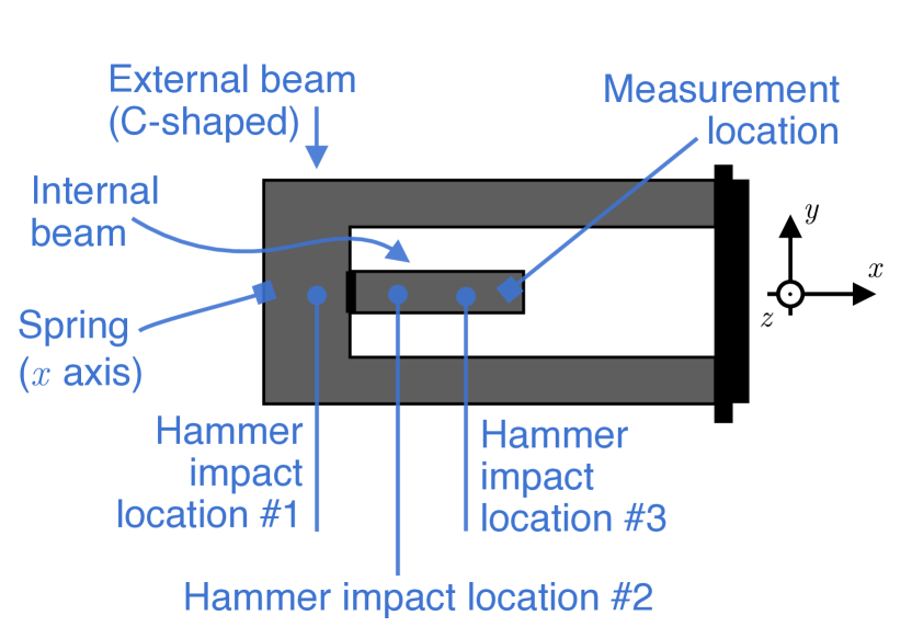
(a)

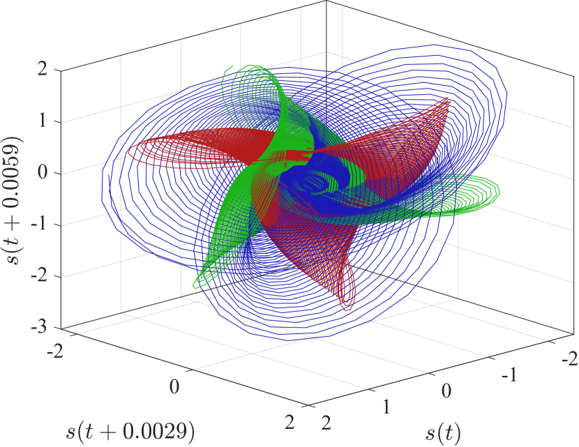
(b)

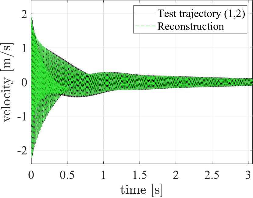
(c)

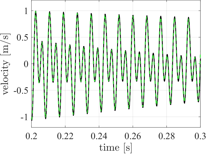
(d)

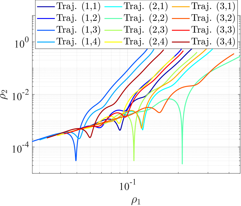
(e)

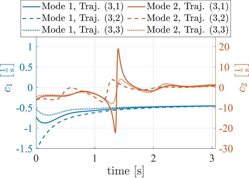
(f)

Figure 6: (6(a)) Sketch of the experimental setup for the resonant beam tester. Cenedese et al. (2022b) (6(b)) The test trajectories embedded in the delay-embedded observable space, in which we fit the SSM. (6(c), 6(d)) The reconstruction from the obtained 4D normal form dynamics agrees with the decay of measured velocities. (6(e)) Plotting the modal amplitudes $\rho$ against one another shows that $\rho_{2}$ dies out more quickly than $\rho_{1}$, but, due to modal interaction, the decay rates vary. (6(f)) The instantaneous damping of the second mode is at times positive, indicating modal energy interchange.

There is, however, a limit to the range of validity of the normal form (36), and so the forced response prediction is not guaranteed to be accurate for arbitrarily high amplitudes. To explore this limitation, we increase the initial point load to 35 kN, equivalent to a maximum displacement of 24.4 mm in the training data. We plot backbone curves computed with fastSSM⁺ at increasing orders in 5(e). For reference, we also compute an approximation of the instantaneous frequency with Peak Finding and Fitting (PFF) from Ref. Jin et al., 2020. Above approximately 20 mm transverse displacement of the beam midpoint, increasing the order of the normal form computation no longer improves the model, as the radius of analyticity seems to be reached. On the other hand, the SSMLearn model remains valid far beyond this limit. This is a clear advantage of the numerical normal form approach in SSMLearn over the analytical computation in fastSSM⁺.

A similar convergence study is shown in 5(f) for increasing orders of SSMTool computation on the full finite-element system of equations. The SSMLearn backbone curve agrees with the PFF estimate at a larger range than SSMTool converges. This shows that data-driven reduced-order modeling can surpass analytical methods in terms of range of validity, even when the full system is known.

IV.3 Resonant beam experiments

Our final dataset comprises velocity measurements from an internally resonant beam structure detailed in Ref. Cenedese et al., 2022b. It consists of an internal beam jointed with three bolts to the left midpoint of an external C-shaped beam, which is clamped to ground at its rightmost edges (6(a)). The bolts give rise to nonlinear frictional slip, Eriten et al. (2013); Brake (2018) and the beam lengths are tuned so that the system has a 1:2 resonance between its slowest out-of-plane bending eigenfrequencies, measured to be 122.4 Hz and 243.4 Hz. Vibrations are induced with an impulse hammer at three different impact locations and the transient out-of-plane velocity of the inner beam tip is measured at 5120 Hz. Varying the impact location and force for data diversity, 12 different trajectories were obtained. Frequency analysis shows that only the two slowest eigenfrequencies are present in the signals, so we aim to identify a 4D internally resonant SSM in an observable space for our model reduction.

With more than one mode present in the data, we must judiciously choose the delay embedding parameters. In the experiment, the sampling time is $\Delta t=0.0001953$ s, which with $\omega_{2}=2\pi\times 243.4$ rad/s produces $\tau=5\Delta t$ according to the method in subsection III.1. This timelag results in a good reconstruction already at the minimum Takens dimension, $p=9$. However, increasing the dimensionality further increases modal orthogonality and thus improves trajectory reconstruction. Motivated by this, we select a delay embedding dimension of $p=12$, as the reconstructions improve only marginally beyond this number. We show a representation of the test trajectories in this observable space in 6(b).

We select three trajectories as the test set – one for each hammer impact location – and use the remaining nine trajectories for training. We set the order of expansion for the SSM $m=3$, the SSM-reduced dynamics order $r=3$, and obtain the 3rd-order normal form. The results do depend on the order of reduced dynamics, but are insensitive to the orders of computation for the SSM and the normal form on it. fastSSM⁺ automatically detects an inner resonance from the data and returns the normal form

$$\dot{\rho}_{1} =-0.4426\rho_{1}+0.0837\rho_{1}\rho_{2}^{2}-5.550\rho_{1}^{3}+$$ (37a)

$$\left(0.2683\cos\psi-0.2639\sin\psi\right)\rho_{1}\rho_{2},$$

$$\rho_{1}\dot{\theta}_{1} =768.9\rho_{1}-0.7541\rho_{1}\rho_{2}^{2}-17.90\rho_{1}^{3}+$$ (37b)

$$\left(-0.2639\cos\psi-0.2683\sin\psi\right)\rho_{1}\rho_{2},$$

$$\dot{\rho}_{2} =-3.125\rho_{2}-4.750\rho_{2}^{3}-12.00\rho_{1}^{2}\rho_{2}+$$ (37c)

$$\left(1.340\cos\psi-0.1161\sin\psi\right)\rho_{1}^{2},$$

$$\rho_{2}\dot{\theta}_{2} =1529\rho_{2}-10.54\rho_{2}^{3}-13.86\rho_{1}^{2}\rho_{2}+$$ (37d)

$$\left(0.1161\cos\psi+1.340\sin\psi\right)\rho_{1}^{2},$$

where $\psi=2\theta_{1}-\theta_{2}$. The reconstruction of the first test trajectory obtained by integrating the normal form is shown in 6(c), with a zoomed-in version in 6(d). The NMTE on the test set computed in the first coordinate is 1.28 %.

6(e) plots the first modal amplitude, $\rho_{1}$, against the second one, $\rho_{2}$, for each simulated trajectory. The second mode clearly decays faster and trajectories are eventually dominated by the slower mode $\rho_{1}$. However, due to the modal coupling terms in the normal form, the decay is not monotonic. Rather, there is a wealth of different decaying patterns depending on initial conditions.

Finally, 6(f) shows the instantaneous damping $\dot{\rho}_{1}/\rho_{1}$ and $\dot{\rho}_{2}/\rho_{2}$ for the reconstructions corresponding to the third impact location. For the slow mode, we observe strong nonlinearity as the instantaneous damping varies dramatically. The fluctuations are even larger for the fast mode. At times, its instantaneous damping reaches positive values, which indicates that energy is transferred from the slow to the fast mode. Sapsis et al. (2012) Overall, the model obtained with fastSSM⁺ agrees with the one returned by SSMLearn in Ref. Cenedese et al., 2022b.

V Conclusions

We have introduced a fast alternative to a recent data-driven reduction method for nonlinear dynamical systems. We have also discussed a simplified implementation for the model reduction setting arising most frequently in practice: a two-dimensional slow SSM with underdamped oscillations modelled up to cubic nonlinearities.

Our approach is fundamentally based on the SSMLearn algorithm, Cenedese et al. (2022a, b) but turns the fitting of an SSM into an explicitly formulated problem by assuming that its tangent space can be obtained by singular value decomposition on the data. Furthermore, we compute the normal form on the manifold explicitly and recursively, rather than solving an implicit minimization problem.

We have applied this simplified model-reduction algorithm to three datasets: tank sloshing experiments, a nonlinear beam finite-element simulation, and experiments from an internally resonant mechanical structure. In all three problems, we obtained a model that accurately predicted the decay of the autonomous system. In addition, we have demonstrated that a forcing term can be added to the autonomous model for highly accurate prediction of the forced response amplitude and phase. Training on the beam experimental data, our method automatically detected the internal resonance and returned a model that could predict energy repartition among the modes.

The assumptions made for our new algorithms drastically speed up model identification on SSMs from data, increase the possible dimensionality of observable spaces we can tackle, and significantly simplify the code. In comparison to the previous method, however, we sacrifice some model accuracy. Perhaps more significantly, we have found large differences in normal form convergence domains to the benefit of SSMLearn.

Specifically, we demonstrate on our simulated beam problem that the numerical normal form has a considerably larger range of validity than the analytical normal forms of the full system and consequently those of our new algorithm. In other words, data-driven analysis can outperform analytical methods in terms of model validity, even when the full equations of the system are known. This suggests that a plausible approach to obtaining a reduced-order model of a finite-element structure would be to simulate the system and train on a small number of trajectories, rather than formulating the full equation system and computing SSMs analytically. This idea is a subject of our ongoing work.

Author declarations

Conflict of interest

The authors have no conflicts to disclose.

References

- Abramian et al. (2020) A. Abramian, E. Virot, E. Lozano, S. Rubinstein, and T. Schneider, “Nondestructive prediction of the buckling load of imperfect shells,” Phys. Rev. Lett. 125, 225504 (2020).
- Holmes et al. (2012) P. J. Holmes, J. L. Lumley, G. Berkooz, and C. W. Rowley, Turbulence, Coherent Structures, Dynamical Systems and Symmetry, 2nd ed., Cambridge Monographs on Mechanics (Cambridge University Press, 2012).
- Lacayo et al. (2019) R. Lacayo, L. Pesaresi, J. Groß, D. Fochler, J. Armand, L. Salles, C. Schwingshackl, M. Allen, and M. Brake, “Nonlinear modeling of structures with bolted joints: A comparison of two approaches based on a time-domain and frequency-domain solver,” Mechanical Systems and Signal Processing 114, 413–438 (2019).
- Taylor (1953) G. Taylor, “An experimental study of standing waves,” Proceedings of the Royal Society of London. Series A. Mathematical and Physical Sciences 218, 44–59 (1953).
- Orosz and Stépán (2006) G. Orosz and G. Stépán, “Subcritical hopf bifurcations in a car-following model with reaction-time delay,” Proc. Royal Soc. A 462, 2643–2670 (2006).
- Kutz and Brunton (2022) J. N. Kutz and S. L. Brunton, “Parsimony as the ultimate regularizer for physics-informed machine learning,” Nonlinear Dynamics 107, 1801–1817 (2022).
- Lumley (1967) J. L. Lumley, “The structure of inhomogeneous turbulent flows,” Atmospheric Turbulence and Radio Wave Propagation , 166–177 (1967).
- Awrejcewicz, Krys’ko, and F. (2004) J. Awrejcewicz, V. A. Krys’ko, and V. A. F., “Order reduction by proper orthogonal decomposition (pod) analysis,” in Nonlinear Dynamics of Continuous Elastic Systems (Springer, Berlin, Heidelberg, 2004) pp. 279–320.
- Schmid (2010) P. Schmid, “Dynamic mode decomposition of numerical and experimental data,” J. Fluid Mech. 656, 5–28 (2010).
- Schmid (2022) P. J. Schmid, “Dynamic mode decomposition and its variants,” Annual Review of Fluid Mechanics 54, 225–254 (2022).
- Kutz et al. (2016) J. N. Kutz, S. L. Brunton, B. W. Brunton, and J. L. Proctor, Dynamic Mode Decomposition (SIAM, Philadelphia, PA, 2016).
- Dylewsky et al. (2022) D. Dylewsky, E. Kaiser, S. L. Brunton, and J. N. Kutz, “Principal component trajectories for modeling spectrally continuous dynamics as forced linear systems,” Phys. Rev. E 105, 015312 (2022).
- Page and Kerswell (2019) J. Page and R. Kerswell, “Koopman mode expansions between simple invariant solutions,” J. Fluid Mech. 879, 1–27 (2019).
- Brunton, Proctor, and Kutz (2016) S. L. Brunton, J. L. Proctor, and J. N. Kutz, “Discovering governing equations from data by sparse identification of nonlinear dynamical systems,” Proceedings of the National Academy of Sciences 113, 3932–3937 (2016).
- Lusch, Kutz, and Brunton (2018) B. Lusch, J. N. Kutz, and S. L. Brunton, “Deep learning for universal linear embeddings of nonlinear dynamics,” Nature Commun. 9, 4950:1–10 (2018).
- Hartman and Mestha (2017) D. Hartman and L. K. Mestha, “A deep learning framework for model reduction of dynamical systems,” in 2017 IEEE Conference on Control Technology and Applications (CCTA) (2017) pp. 1917–1922.
- Daniel et al. (2020) T. Daniel, F. Casenave, N. Akkari, and D. Ryckelynck, “Model order reduction assisted by deep neural networks (rom-net),” Adv. Model. and Simul. in Eng. Sci. 7, 105786 (2020).
- Loiseau, Brunton, and Noack (2020) J.-C. Loiseau, S. L. Brunton, and B. R. Noack, “From the pod-galerkin method to sparse manifold models,” in Model Order Reduction, Volume 3: Applications, edited by P. Benner, S. Grivet-Talocia, A. Quarteroni, G. Rozza, W. Schilders, and L. M. Silveira (De Gruyter, Berlin, 2020) pp. 279–320.
- Haller and Ponsioen (2016) G. Haller and S. Ponsioen, “Nonlinear normal modes and spectral submanifolds: existence, uniqueness and use in model reduction,” Nonlinear Dyn. 86, 1493–1534 (2016).
- Szalai (2020) R. Szalai, “Invariant spectral foliations with applications to model order reduction and synthesis,” Nonlinear Dyn. 101, 2645–2669 (2020).
- Jain et al. (2021) S. Jain, T. Thurner, M. Li, and G. Haller, “SSMTool: Computation of invariant manifolds and their reduced dynamics in high-dimensional mechanics problems.” (2021).
- Ponsioen, Pedergnana, and Haller (2018) S. Ponsioen, T. Pedergnana, and G. Haller, “Automated computation of autonomous spectral submanifolds for nonlinear modal analysis,” J. Sound and Vibration 420, 269–295 (2018).
- Ponsioen, Jain, and Haller (2020) S. Ponsioen, S. Jain, and G. Haller, “Model reduction to spectral submanifolds and forced-response calculation in high-dimensional mechanical systems,” J. Sound and Vibration 488, 115640 (2020).
- Jain, Tiso, and Haller (2018) S. Jain, P. Tiso, and G. Haller, “Exact nonlinear model reduction for a von Kármán beam: slow-fast decomposition and spectral submanifolds,” Journal of Sound and Vibration 423, 195–211 (2018).
- Jain and Haller (2021) S. Jain and G. Haller, “How to compute invariant manifolds and their reduced dynamics in high-dimensional finite element models,” Nonlinear Dynamics 107, 1417–1450 (2021).
- Li, Jain, and Haller (2021) M. Li, S. Jain, and G. Haller, “Nonlinear analysis of forced mechanical systems with internal resonance using spectral submanifolds – part I: Periodic response and forced response curve,” (2021), arXiv:2106.05162 [math.DS] .
- Li and Haller (2021) M. Li and G. Haller, “Nonlinear analysis of forced mechanical systems with internal resonance using spectral submanifolds – part II: Bifurcation and quasi-periodic response,” (2021), arXiv:2108.08152 [math.DS] .
- Szalai, Ehrhardt, and Haller (2017) R. Szalai, D. Ehrhardt, and G. Haller, “Nonlinear model identification and spectral submanifolds for multi-degree-of-freedom mechanical vibrations,” Proc. Royal Society A 473, 20160759 (2017).
- Cenedese et al. (2022a) M. Cenedese, J. Axås, B. Bäuerlein, K. Avila, and G. Haller, “Data-driven modeling and prediction of non-linearizable dynamics via spectral submanifolds,” Nat. Commun. 13 (2022a), 10.1038/s41467-022-28518-y.
- Guckenheimer and Holmes (1983) J. Guckenheimer and P. Holmes, Nonlinear Oscillations, Dynamical Systems and Bifircation of Vector Fields (Springer, New York, 1983).
- Cenedese et al. (2022b) M. Cenedese, J. Axås, H. Yang, M. Eriten, and G. Haller, “Data-driven nonlinear model reduction to spectral submanifolds in mechanical systems,” Phil. Trans. R. Soc. A (2022b), in press.
- Kaszás, Cenedese, and Haller (2022) B. Kaszás, M. Cenedese, and G. Haller, “Dynamics-based machine learning of transitions in couette flow,” (2022).
- Cabré, Fontich, and de la Llave (2003) Cabré, E. Fontich, and R. de la Llave, “The parameterization method for invariant manifolds I: Manifolds associated to non-resonant subspaces,” Indiana Univ. Math. J. 52, 283–328 (2003).
- Cenedese, Axås, and Haller (2021) M. Cenedese, J. Axås, and G. Haller, “SSMLearn,” (2021).
- Fornberg (1988) B. Fornberg, “Generation of finite difference formulas on arbitrarily spaced grids,” Mathematics of Computation 51, 699–706 (1988).
- Takens (1981) F. Takens, “Detecting strange attractors in turbulence,” in Dynamical Systems and Turbulence, Warwick 1980, edited by D. Rand and L. Young (Springer Berlin Heidelberg, 1981) pp. 366–381.
- Sauer, Yorke, and Casdagli (1991) T. Sauer, J. Yorke, and M. Casdagli, “Embedology,” J. Stat. Phys. 65, 579–616 (1991).
- Deyle and Sugihara (2011) E. R. Deyle and G. Sugihara, “Generalized theorems for nonlinear state space reconstruction,” PLoS ONE 6 (2011).
- Breunung and Haller (2018) T. Breunung and G. Haller, “Explicit backbone curves from spectral submanifolds of forced-damped nonlinear mechanical systems,” Proc. Royal Soc. A 474, 20180083 (2018).
- Ponsioen, Pedergnana, and Haller (2019) S. Ponsioen, T. Pedergnana, and G. Haller, “Analytic prediction of isolated forced response curves from spectral submanifolds,” Nonlinear Dyn. 98, 2755–2773 (2019).
- Faltinsen and Timokha (2009) O. Faltinsen and A. Timokha, Sloshing (Cambridge University Press, 2009).
- Cheli et al. (2013) F. Cheli, V. D’Alessandro, A. Premoli, and E. Sabbioni, “Simulation of sloshing in tank trucks,” International Journal of Heavy Vehicle Systems 20, 1–16 (2013).
- Dodge (2000) F. Dodge, The New "Dynamic Behavior of Liquids in Moving Containers" (Southwest Research Inst., 2000).
- Abramson (1966) H. Abramson, ed., The dynamic behavior of liquids in moving containers: with applications to space vehicle technology, NASA SP-106 (Scientific and Technical Information Division, National Aeronautics and Space Administration, Washington, D.C, 1966).
- Bäuerlein and Avila (2021) B. Bäuerlein and K. Avila, “Phase lag predicts nonlinear response maxima in liquid-sloshing experiments,” J. Fluid Mech. 925, A22 (2021).
- Jin et al. (2020) M. Jin, W. Chen, M. R. W. Brake, and H. Song, “Identification of Instantaneous Frequency and Damping From Transient Decay Data,” Journal of Vibration and Acoustics 142 (2020), 10.1115/1.4047416.
- Eriten et al. (2013) M. Eriten, M. Kurt, G. Luo, D. D. McFarland, L. Bergman, and A. Vakakis, “Nonlinear system identification of frictional effects in a beam with a bolted joint connection,” Mechanical Systems and Signal Processing 39, 245–264 (2013).
- Brake (2018) M. Brake, The mechanics of jointed structures: recent research and open challenges for developing predictive models for structural dynamics (Springer International Publishing, 2018).
- Sapsis et al. (2012) T. Sapsis, D. Quinn, A. Vakakis, and L. Bergman, “Effective stiffening and damping enhancement of structures with strongly nonlinear local attachments,” Journal of Vibration, Acoustics, Stress, and Reliability in Design 134 (2012), 10.1115/1.4005005.