Symbolic analysis meets federated learning to enhance malware identifier

Abstract.

Over past years, the manually methods to create detection rules were no longer practical in the anti-malware product since the number of malware threats has been growing. Thus, the turn to the machine learning approaches is a promising way to make the malware recognition more efficient. The traditional centralized machine learning requires a large amount of data to train a model with excellent performance. To boost the malware detection, the training data might be on various kind of data sources such as data on host, network and cloud-based anti-malware components, or even, data from different enterprises. To avoid the expenses of data collection as well as the leakage of private data, we present a federated learning system to identify malwares through the behavioural graphs, i.e., system call dependency graphs. It is based on a deep learning model including a graph autoencoder and a multi-classifier module. This model is trained by a secure learning protocol among clients to preserve the private data against the inference attacks. Using the model to identify malwares, we achieve the accuracy of $\sim 85\%$ for the homogeneous graph data and $\sim 93\%$ for the inhomogeneous graph data.

1. Introduction

Since the number of malware threats has been growing over past years, the manually analysis methods to create detection rules were no longer practical in the anti-malware product. It thus requires the new advanced protection techniques which optimize the tasks of malware detection and classification. Hence, the turn to the machine learning (ML) approaches is a promising way to make the malware recognition more efficient, robust and scalable (Lab, 2021; Singh and Singh, 2021). In the traditional centralized ML, a large amount of data is required to train a model with excellent performance. To boost the malware detection, it might train the model on various kinds of data sources such as data on host, network and cloud-based anti-malware components, or even, data from different enterprises since the amount of data on each side is insufficient. Although all data can be collected in a central server for training, it is too expensive as well as it might cause the leakage of sensitive data (Abadi et al., 2016; Li et al., 2018).

To tackle this challenge, there are serveral works (Lin and Huang, 2020; Payne and Kundu, 2019; Rey et al., 2022b; Li et al., 2021; Zhang et al., 2021; Zhao et al., 2019; Nguyen et al., 2019) which implement the federated learning (FL) which pushes model training to the devices from which data originate. Each device uses local data to train the local model, and then, all the local models are sent to the server to be aggregated into a global model. This FL setting is risk in preserving data privacy since the sensitive information of the local data may be revealed via the inference attacks to training model (Wang et al., 2018; Zhu et al., 2019; Melis et al., 2019). Hence, an additional privacy protection is setup to the FL with amount of differential privacy noise adding to the model parameters (Abadi et al., 2016). However, the work in (Boenisch et al., 2021) shows that relying on the differential privacy noise is insufficient to prevent the data leakage via the training model, as they explicitly trust the server with the crucial task of adding the differential privacy noise, and thus provide no protection against a semi-honest or untrusted server. In other hand, the more differential privacy noise is added to the model, the more degraded the performance of FL.

Taking into account these issues, we introduce a FL system that enables multiple participants to jointly learn a accurate deep learning model for malware detection and classification without sharing their input datasets while preserving privacy of the local data against the inference attacks. Our system consists of clients which hold their own datasets, a key-client which holds the secret key to encrypt the model parameters, and an aggregator which combines the local model parameters into a global model. To avoid the inference data attack, we replace the key-client for every training round. Even the aggregator or clients take snapshot of the training model, it is hard for them to infer the data from others. In particular, each client holds its own classifier model which is trained to recognize malwares at the clients’ side. For this goal, we first characterise malwares by the system call dependency graphs (SCDG) which represent the program behaviours. Following  (Sebastio et al., 2020; Bertrand Van Ouytsel and Legay, 2021; Namani and Khan, 2020), we implement the symbolic analysis to explore all possible execution paths of a malware, and then, its corresponding SCDG is built from these execution paths. Second, we propose a deep learning model including a graph autoencoder and a multi-classifier, to encode and classify the SCDGs. The graph autoencoder vectorizes the input SCDGs, and then, the multi-classifier identifies malwares according to the output of the autoencoder. We evaluate the deep learning model on two datasets. The first dataset includes SCDGs computed by the same extraction strategy. The second dataset includes SCDGs computed by different strategies. In the experiment, we obtain significant results which are comparable to the Centralized Learning. The accuracy is $\sim 85\%$ for the homogeneous graphs. It can achieve $\sim 93\%$ for the inhomogeneous graphs.

Section 2 presents related works. Then, we recall the definition of system call dependency graph, and present the symbolic analysis to extract the graphs from malwares in Section 3. Section 4 presents the Deep neural classifier which we propose for encoding and classifying the system call dependency graphs. Our secure learning approach to train the deep learning model is introduced in Section 5. Section 6 reports its evaluation results on our datasets. Finally, the conclusion is presented in Section 7.

2. Related work

Malware detection approaches are mainly categorized into signature based and behavioural based approaches. The signature based approaches extract binary patterns for a malware family, and use these patterns to detect all samples of that family. The approaches suffer from building a huge database of signatures within a short period of time as well as they can not be used to detect new malware families. In addition, it is very easy to be overtaken by deforming or obfuscating the binaries. In the latter more advanced approaches, they detect malware by analyzing its behaviours instead of the syntax of the program. The behavioural analysis is usually distinguished as dynamic or static analysis. In the dynamic analysis (Egele et al., 2008), malwares are executed in an emulated environment, e.g., sandbox, to look for a malicious behaviour (Willems et al., 2007). It is hard to trigger the malicious behaviour since there are limitation in execution time and the context emulated by the sandbox.

On the other hand, static techniques allow to analyze the behaviours of malware on the disassembled code without executing it. The static code analysis is performed concretely or symbolically. In the concrete analysis (Gritti et al., 2020), the execution trace is computed from the disassembled code by some contextual information. Therefore, it has similar limitations to the dynamic analysis since the provided contexts cannot cover all the executions of program. The symbolic analysis performs a symbolic execution with symbolic input variables in place of concrete values. It allows exploring all the possible execution paths in the control flow graph (Sebastio et al., 2020; Bertrand Van Ouytsel and Legay, 2021; Namani and Khan, 2020). Thus, the malicious behaviours are easily exposed in this analysis. We consider the symbolic analysis in this work to construct SCDGs as behavioural signatures of malware. This behavioural graph representation has been proved as a good approach for malware detection in the recent works (Dam and Touili, 2016; Said et al., 2018; Bertrand Van Ouytsel and Legay, 2021; Fredrikson et al., 2010; Lajevardi et al., 2021; Macedo and Touili, 2013; Dam et al., 2021).

(Dam and Touili, 2016; Bertrand Van Ouytsel and Legay, 2021) implement machine learning techniques on SCDGs for malicious behaviour extraction as well as malware detection. The graph mining techniques are employed to find malicious patterns in SCDGs of malwares in (Said et al., 2018; Fredrikson et al., 2010; Macedo and Touili, 2013; Lajevardi et al., 2021). (Dam et al., 2021) identifies malware families by applying the clustering algorithm on SCDGs. Those works obtain good results in the malware detection and classification. However, there are several challenges in training and updating the malware classifiers since malware detectors need to be updated consistently with a mass number of malwares. In addition, collecting all data in a centralized manner are so expensive while the data on individual devices are insufficient for training the efficient machine learning model. Therefore, the federated learning is proposed to handle the issues in the traditional machine learning (Konečnỳ et al., 2016). It requires each device to use local data to train the local model, and then all the local models are uploaded to the server to be aggregated into a global model. This learning techinque is successfully applied for anomaly detection (Nguyen et al., 2019; Rey et al., 2022a; Ghimire and Rawat, 2022) as well as malware detection (Lin and Huang, 2020; Hsu et al., 2020; Gálvez et al., 2020). (Nguyen et al., 2019; Rey et al., 2022a; Ghimire and Rawat, 2022) successfully employ the federated learning techniques for anomaly detection on IoT devices. (Lin and Huang, 2020) also shows the positive efficiency of the federated learning for malware classification comparing to the traditional machine learning, i.e., support vector machine (SVM). However, it is lack of the private data protection. Moreover, the privacy-preserving federated learning system is implemented in (Hsu et al., 2020; Gálvez et al., 2020). (Hsu et al., 2020) allows mobile devices to collaborate together for training a SVM classifier with a secure multi-party computation technique. (Gálvez et al., 2020) implements an average weight model to preserving the data privacy. Enhancing the models in (Gálvez et al., 2020; Hsu et al., 2020), we implement a secure learning approach with the homomorphic encryption to avoid the data inference attacks. Additionally, we implement a federated learning on inhomogeneous SCDGs to exploit the computation power of devices as well as the various representations of malware behaviours.

3. System call dependency graph

System call dependency graph (SCDG) is a directed graph consisting of nodes and edges, that represents the beahviours of a program. The nodes are (system) function calls. An edge represents information flowing between two two system calls in execution traces. The execution traces are obtained through the symbolic execution of a binary. Each trace is a list of system calls and the relevant information of these calls, such as the arguments, the resolved address and the calling address. Two system calls on an execution trace are data dependent if they are either argument relationship or address relationship. Two system calls have the argument relationship if they are using the same argument in an execution trace. The address relationship of two system calls is when an argument of a system call is the return value of another call.

Let $S$ be a set of system calls. Formally, a system call dependency graph is a directed graph $G=(V,E,L)$ such that: $V$ is a set of nodes, $L:V\rightarrow S$ is a labelling function which maps a node $v\in V$ to a system call $s\in S$ and $E:V\times V$ is set of edges. $(v_{1},v_{2})\in E$ means that the system calls $L(v_{1})$ and $L(v_{2})$ are data dependent and the call to $L(v_{1})$ is made before the call to $L(v_{2})$, e.g., the argument relationship of two system calls GetModuleFilenameA(0,m) and CopyFileA(m,m’,1) is represented by an edge $(v_{1},v_{2})\in E$ in the graph $G=(V,E)$ such as $v_{1},v_{2}\in V$, $L(v_{1})=\texttt{GetModuleFilenameA}$ and $L(v_{2})=\texttt{CopyFileA}$.

In this work, we implement a symbolic execution to extracte SCDGs from the binaries as follows. First, the symbolic execution is performed on malware binaries to explore all possible execution paths. Thanks to angr engine (Shoshitaishvili et al., 2016), the execution flows of the binary are recorded as states including the instruction addresses, register values, memory usages, etc. in a period of time. At each execution step, if a variable can take several values, the symbolic value is replaced to keep track the execution and the related constraints. During the execution, the new states are created according to the instruction by the angr engine. If the branch instruction, i.e., the conditional jump, the current state is forked into two states: the first is considered for taking the jump instruction, and the second is considered for the next instruction. Otherwise, the current state produces a single child state. Hence, the exploration will produce a huge number of states during the symbolic execution. The state explosion can be controlled by using some constraint solvers, i.e., z3 or SMT solver, or heuristics to optimize the symbolic execution (Sebastio et al., 2020). Following (Bertrand Van Ouytsel and Legay, 2021), we consider three strategies to explore the state at each execution step to compute SCDGs:

1. Custom Breadth-first search (CBFS) implements the Breadth-first search to construct the graph of possible shortest paths from the execution traces.

2. Custom Depth-first search (CDFS) considers the possible longest paths in the Depth-first search on the execution traces.

3. Breadth-first search (BFS) explores all paths from the execution traces in the Breadth-first search manner.

After the state exploration, we obtain serveral execution traces from a binary. Each trace is a sequence of system calls with the arguments, the resolved addresses and the calling addresses. Then, a SCDG is built on these execution traces. Its nodes correspond to system calls. Its edges represent the information flow of pair of system calls and their order in the execution traces. An edge is built from two system calls if they are either the argument relationship or the address relationship in the same execution trace. By using different exploration strategies, we may obtain various SCDGs to characterise the same binary. Hence, the study on such various SCDGs may boost the performance of malware detection as well as malware family recognition.

4. Deep learning model

Since the SCDGs correspond to the behaviours of malware, we construct a deep learning model in order to encoding the SCDGs and classifying the malware. The model consists in a graph autoencoder connecting to a classifier module, shown in Figure 1. First, the graph autoencoder transforms a SCDG into a feature vector. Then, the classifier module takes the feature vector as input, and produces a predicted class of SCDG associated with this feature vector. They are presented in the following sections.

Figure 1. Deep neural network classifier

4.1. Graph autoencoder

The graph autoencoder (Dam et al., 2021) is equipped with Long Short Term Memory (LSTM) layers to embedding a SCDG into a feature vector. A LSTM layer is a recurrent neural network which is able to remember information for a long periods of times through memory cells. Each cell has three connected gates to control the internal state: the input gate $i_{t}$ is used to decide which part of information is stored in the memory cell; the forget gate $f_{t}$ is used to decide which part of information is thrown away from the memory cell; and the output gate $o_{t}$ which specifies the output. Given an input $x_{t}$ and the output of previous cell $h_{t-1}$, the output $h_{t}$ is computed by $h_{t}=o_{t}\ast\textbf{tanh}(C_{t})$. $C_{t}$ is the internal state of the current cell is computed as follows:

$$C_{t}=f_{t}\ast C_{t-1}+i_{t}\ast\tilde{C}_{t}$$

where $\tilde{C}_{t}=\textbf{tanh}(W_{C}\cdot[h_{t-1},x_{t}]+b_{C})$ is a new candidate for the internal state. Over periods of time, three gates of the memory cell are interacting layers with the sigmoid function $\sigma(\cdot)$ as follows:

$$f_{t}=\sigma(W_{f}\cdot[h_{t-1},x_{t}]+b_{f})$$

$$i_{t}=\sigma(W_{i}\cdot[h_{t-1},x_{t}]+b_{i})$$

$$o_{t}=\sigma(W_{o}\cdot[h_{t-1},x_{t}]+b_{o})$$

where $\{W_{f},W_{i},W_{o}\}$ and $\{b_{f},b_{i},b_{o}\}$ are weights and biases of corresponding layers. These $\{W_{f},W_{i},W_{o}\}$ and $\{b_{f},b_{i},b_{o}\}$ are also called model parameters.

Let $\operatorname*{\mathbf{G}}$ be a SCDG. The graph autoencoder trains its LSTM layers through two modules: The encoder module $\operatorname*{\mathbf{E}(\mathbf{G})}$ transforms the graph structure, i.e., possible paths in $\mathbf{G}$, into a feature vector, i.e.,$\operatorname*{\mathbf{x}}=\operatorname*{\mathbf{E}(\mathbf{G})}$. The decoder module $\operatorname*{\mathbf{D}(\mathbf{x})}$ does an opposite way to reconstruct the original graph $\operatorname*{\mathbf{\widehat{G}}}$ from its feature vector $\operatorname*{\mathbf{x}}$ given by the encoder module, i.e., $\operatorname*{\mathbf{\widehat{G}}}=\operatorname*{\mathbf{D}(\mathbf{x})}$. This graph autoencoder is trained to optimize a reconstruction error $\text{Loss}_{1}$:

$$\text{Loss}_{1}(\operatorname*{\mathbf{G}},\operatorname*{\mathbf{\widehat{G}}})=\frac{1}{2}\sum_{i=1}^{n}||c_{i}-\hat{c}_{i}||^{2}$$

where $||c_{i}-\hat{c}_{i}||$ is the differency measure of the component $c_{i}$ of the original graph $\operatorname*{\mathbf{G}}$ and its reconstructed component $\hat{c}_{i}$ in the graph $\operatorname*{\mathbf{\widehat{G}}}$. Using LSTM layers as its internal layers enables the graph autoencoder featuring arbitrary size graphs, i.e., SCDGs.

4.2. Classifier module

The classifier module is a combination of $n$ single classifiers, i.e., $\{\mathbf{F}_{i}(\mathbf{x})\}^{n}_{i=1}$, $n>0$. Each classiifer $i$ corresponds to a malware family. It is a fully connected neural network layer connected to the activation function $\text{softmax}(\cdot)$ (Goodfellow et al., 2016). These classifiers are connected to the graph autoencoder via the output of the encoder $\operatorname*{\mathbf{E}(\mathbf{G})}$. Let $\operatorname*{\mathbf{x}}$ be an output of $\operatorname*{\mathbf{E}(\mathbf{G})}$. The module is defined as follows:

$$\hat{y}=\text{softmax}([\mathbf{F}_{i}(\mathbf{x})]^{n}_{i=1})$$

$$\operatorname*{\mathbf{L}}(\operatorname*{\mathbf{x}})=\operatorname*{arg\,max}^{n}_{i=1}(\hat{y})$$

where $\operatorname*{\mathbf{L}}(\operatorname*{\mathbf{x}})$ is the predicted label class of SCDG indicating the predicted malware family, $\mathbf{F}_{i}(\mathbf{x})=\mathbf{W}_{i}\cdot\operatorname*{\mathbf{x}}+\mathbf{b}_{i}$. $\mathbf{W}_{i}$ and $\mathbf{b}_{i}$ respectively are weight and bias values of the layer $\mathbf{F}_{i}$. The $\{(\mathbf{W}_{i},\mathbf{b}_{i})\}_{i=1}^{n}$ are model’s parameters.
This module is trained to optimize the Binary Cross Entroy Loss:

$$\text{Loss}_{2}=-\frac{1}{n}\sum_{i=1}^{n}y_{i}\log(\hat{y}_{i})+(1-y_{i})\log(1-\hat{y}_{i})$$

where $y$ specifies the ground truth class of SCDG associated with $\operatorname*{\mathbf{x}}$. $y_{i}=1$ if the SCDG is in the class $i$. Otherwise, $y_{i}=0$.

To train the deep learning model, we use a stochastic optimization algorithm, i.e., Adam optimization algorithm (Kingma and Ba, 2014), which recomputes the model parameters in very training step on the training data, in order to optimizing the total loss function. The total loss function Loss is a sum of losses from the graph autoencoder and the classifier module.

$$\text{Loss}=\text{Loss}_{1}+\text{Loss}_{2}.$$

5. Secure learning approach

In the previous section, we introduce the deep learning model to classify SCDGs. We present in this section a secure learning approach to train this model on different devices/clients using the concept of federated learning. We first recall the federated learning (FL) (Konečnỳ et al., 2016). FL is a collaboratively learning among N devices/clients with the help of a central server, e.g., an aggregator server. In the training process, clients use their private dataset to train their local model, and then, all the local models are sent to the aggregator server to be aggregated for a global model. Then, the parameters of the global model are sent to clients for updating to their local model. After a sufficient number of local training and updates exchanges between the aggregator server and the associated clients, the clients’ models can converge to an optimal learning model. However, the FL is not always a sufficient privacy mechanism to protect the privacy of clients, i.e., the private dataset. It is easy to be exposed to the data inference attacks. As we have mentioned above, the popular technique, such as using differential privacy to protect the private data, is not strong enough to protect the leakage of private data (Boenisch et al., 2021). In addition, using encryption algorithms, such as using homomorphic encryption (Phong et al., 2018; Aono et al., 2016), multi-party computating (MPC) (Burkhart et al., 2010), is more potential ways to preserve the data privacy. In the section, we implement a secure learning protocol with an average-weight aggregation using homomorphic encryption. It protects the private data from semi-honest clients and server. Note that the semi-honest (a.k.a honest-but-curious) model is that collaborators (clients/server) do follow the protocol but try to infer as much as possible from the values (shares) they learn, also by combining their information. This protocol is presented in the following sections.

5.1. Communication setting

We implement an asymmetric encryption for the communication between clients and the server (Figure 2). Support a client want to send safely a message to the server. First, the server generates a key pair composed of a private key and a public key. The private key is hidden by the server. The public key is openly distributed to the client. The private key can decrypt what the public key encrypts, and vice versa. Then, the client encrypts its message by using the server’s public key. It openly sends this ciphertext to the server. This ciphertext is safe since any other cannot decrypts it without the private key from the server. Server receives the ciphertext and decrypts it with its private key. Thus, this setting ensures a secure communication between the client and the server.

Figure 2. Client-Server communication

5.2. Homomorphic encryption for a secure training model

For a safe computation at the aggregator, we implement the homorphic encryption to the model parameters. let us recall the homomorphic encryption scheme (Regev, 2009; Chowdhary et al., 2021; Kim et al., 2020). Let $(\mathbf{sk},\mathbf{pk})$ be a pair of secret and public keys, respectively. Given a numeric value $\mathbf{z}$. First, $\mathbf{z}$ is encoded into a plaintext. The public key $\mathbf{pk}$ is used to encrypt the plaintext of $\mathbf{z}_{plaintext}$ into a ciphertext $\bar{z}_{\mathbf{pk}}$. Let HEnc be a function which encodes a numeric value and encrypts its plaintext into a ciphertext with a public key, e.g., $\bar{z}_{\mathbf{pk}}=\text{HEnc}(\mathbf{z},\mathbf{pk})$. Let HDecrypt be a function which decrypts a ciphertext by using a secret key and decodes its plaintext into a numeric value. Then, $\text{HDecrypt}(\bar{z}_{\mathbf{pk}},\mathbf{sk})$ decrypts $\bar{z}_{\mathbf{pk}}$ to the plaintext $\mathbf{z}_{plaintext}$, and it decodes $\mathbf{z}_{plaintext}$ to the numeric value $\mathbf{z}$, i.e., $\mathbf{z}=\text{HDecrypt}(\bar{z}_{\mathbf{pk}},\mathbf{sk})$.

The important property of homomorphic encryption is that users can process and calculate the encrypted data without revealing the original data. With the secret key, the user decrypts the processed data, which is exactly the expected result (Chen et al., 2018; Nikolaenko et al., 2013). Given numeric values $\mathbf{x}$ and $\mathbf{z}$, the multiplication of the ciphertext of $\mathbf{z}$, i.e., $\bar{z}_{\mathbf{pk}}$, and the plaintext of $\mathbf{x}$, i.e., $\mathbf{x}_{plaintext}$, is a ciphertext of $\mathbf{z}\cdot\mathbf{x}$, i.e., $\text{HEnc}(\mathbf{z}\cdot\mathbf{x},\mathbf{pk})=\bar{z}_{\mathbf{pk}}\cdot\mathbf{x}_{plaintext}$. The addtion of two ciphertexts $\bar{x}_{\mathbf{pk}}$ and $\bar{z}_{\mathbf{pk}}$ is also a ciphertext of $\mathbf{z}+\mathbf{x}$, i.e., $\text{HEnc}(\mathbf{z}+\mathbf{x},\mathbf{pk})=\bar{z}_{\mathbf{pk}}+\bar{x}_{\mathbf{pk}}$.

With the homomorphic encryption, we implement a secure learning among N clients. The local updates is protected in the encrypted message. The global update is computing on encrypted data with respect to the addition operator of the homomorphic encryption. The Algorithm 1 describes the $m$ training rounds of N clients. Each client $i$ holds a pair of $(\mathbf{pk}^{i},\mathbf{sk}^{i})$, and the Key-client holds a secret value $\mathbf{z}$. For each training round, the training process is as follows: First, the system selects a Key-client among clients. The selected client, i.e., Key-client, exchange the public key, i.e., $\mathbf{pk}^{i}$, and its encrypted value, i.e., $\bar{z}_{\mathbf{pk}^{s}}=\text{HEnc}(\mathbf{z},\mathbf{pk}^{s})$ with other clients. Meanwhile, each client locally trains their local model. When the training step is done, they use the ciphertext $\bar{z}_{\mathbf{pk}^{s}}$ of the Key-client to encrypt the parameters of their local model and send to the aggregator. Then, the aggregator computes the sum of clients’s parameters, and sends to the Key-client. The Key-client decrypts the global updates from the aggregator, i.e., $\mathbf{w}=\frac{1}{\mathbf{z}\cdot\mathbf{N}}\text{Decrypt}(\bar{w}_{\mathbf{pk}^{s}})$ and sends the updates $\mathbf{w}$ to every client $i$. Finally, the clients receive and apply the updates to their local model. After these updates are done, a new round is started by voting a new Key-client and training the local models at the clients’ side.

1:for each $round\in[1\ldots m]$  do

2:     Randomly vote a Key-client among clients.

3:     The clients send their public keys, i.e., $\mathbf{pk}^{i}$, to the Key-client.

4:     The Key-client sends its encrypted secret value $\bar{z}_{\mathbf{pk}^{s}}=\text{HEnc}(\mathbf{z},\mathbf{pk}^{s})$ to all clients.

5:     for each $i\in[1\ldots\mathbf{N}]$  do in parallel

6:         The client $i$ trains the local model on its own data.

7:         The client $i$ encrypts the model’s parameters $\mathbf{w}^{i}$ using the secret value $\bar{z}_{\mathbf{pk}^{s}}$, i.e., $\bar{w}^{i}_{\mathbf{pk}^{s}}=\mathbf{w}^{i}\cdot\bar{z}_{\mathbf{pk}^{s}}$.

8:         The client $i$ sends the update $\bar{w}^{i}_{\mathbf{pk}^{s}}$ to the aggregator.

9:     end for

10:     The aggregator computes the encrypted global weight

$$\bar{w}_{\mathbf{pk}^{s}}=\sum_{i=1}^{n}\bar{w}^{i}_{\mathbf{pk}^{s}}.$$

11:     The aggregator sends the encrypted global weight $\bar{w}_{\mathbf{pk}^{s}}$ to the Key-client.

12:     The Key-client decrypts $\bar{w}_{\mathbf{pk}^{s}}$ by its secret key $\mathbf{sk}^{s}$ and the secret value $\mathbf{z}$ to get the global weight $\mathbf{w}$.

$$\mathbf{w}=\frac{1}{\mathbf{z}\cdot\mathbf{N}}\text{HDecrypt}(\bar{w}_{\mathbf{pk}^{s}},\mathbf{sk}^{s})$$

13:     for each $i\in[1\ldots\mathbf{N}]$  do in parallel

14:         The Key-client encrypts the updates $\mathbf{w}$ by $\mathbf{pk}^{i}$, i.e., $\mathbf{w}_{\mathbf{pk^{i}}}$, and sends the updates to the client $i$.

15:         The client $i$ decrypts $\mathbf{w}_{\mathbf{pk^{i}}}$ by its secret key $\mathbf{sk}^{i}$ and applies the updates to its local model.

16:     end for

17:end for

Algorithm 1 Secure training in the federated learning

5.3. Application to malware identifier

We apply the secure learning protocol to train the deep learning model on $N$ clients. Each client has its own malwares which cannot be shared to others. To identify malwares, the clients implement a classifier model at their side. They share the parameters of their local classifier model during the training phase. They get back the update from the aggregator after each training round. An example of the training process of 3 clients is shown in Figure 3: Clients keep their binaries/malwares. Using the SCDG extraction, they generate SCDGs from their binaries, and the SCDGs are also kept in private. Then, they train the local model on the extracted SCDGs. The trained model’s parameters are encrypted, and they are sent to aggregator. The aggregator safely computes the update on the encrypted parameters. Then, it sends the aggregated parameters to the Key-client, i.e., Client-2, for decryption. The Key-client decrypts the aggregated parameters, and sends them to Client-1 and Client-3. The clients receive the aggregated parameters, and update to the local model. The communication channels among the aggregator and clients are implemented following the client-server communication in Section 5.1.

In this work, we consider two cases of sharing the model paramaters as follows:

1. Clients collaboratively learn the full model including the graph autoencoder $(\operatorname*{\mathbf{E}(\mathbf{G})},\operatorname*{\mathbf{D}(\mathbf{x})})$ and the classifier module $\{\mathbf{F}_{i}(\cdot)\}$, called Full-Aggregation Learning. This is a closed collaboration since all clients should have the same structure of their local model as well as they share their data labels.

2. We decompose the model in Section 4 into two parts: the autoencoder $(\operatorname*{\mathbf{E}(\mathbf{G})},\operatorname*{\mathbf{D}(\mathbf{x})})$ and the classifier module $\{\mathbf{F}_{i}(\cdot)\}$. Clients share only a part of model, i.e., the encoder part $\operatorname*{\mathbf{E}(\mathbf{G})}$, with each other, called Partly-Aggregation Learning. It enables clients sharing their feature computing in the form of an encoder $\operatorname*{\mathbf{E}(\mathbf{G})}$. Thus, it keeps the private data classes. It then allows a flexible implement of learning paradigms at the client’s side.

Figure 3. Secure learning among $3$ clients and one aggregator. Client-2 is the Key-Cient, and it might be replaced by another after each training round.

6. Experiment

We evaluate the performance of our deep learning system in this section. We first present our datasets and the data proportion on each client. Then, we present the implement of our learning approaches on the homogeneous SCDGs and on the inhomogeneous SCDGs. The results also are compared the implement of the Centralized Learning. The FL experiment is deployed on 4 virtual machines. Their resources are reported in Table 1.

	Physical CPU	Virtual CPU	Memory
Aggregator	4	8	24GB
Client-1	4	8	24GB
Client-2	8	8	20GB
Client-3	8	8	15GB

Table 1. Virtual Machines used in our experiment

The evaluation is measured by the accuracy of the trained malware identifier as follows:

$$\text{Accuracy}(y,\hat{y})=\frac{1}{n}\sum_{i=1}^{n}1(y_{i}=\hat{y}_{i})$$

where $n$ is the number of samples, $1(\cdot)$ is the indicator function, $\hat{y}_{i}$ is the predicted value of the i-th sample and $y_{i}$ is the corresponding true value.

6.1. Dataset

We collect malwares from Cisco and MalwareBazaar Database  to build two datasets: Dataset-1 and Dataset-2. Dataset-1 consists of 2260 malwares from 15 families. It is randomly splitted into two sets: the training set of 2034 malwares and the test set of 226 malwares. The SCDGs in Dataset-1 are computed by the same strategy, i.e., CDFS which is presented in Section 3. Dataset-1 is used for the Homogeneous-data scheme. Dataset-2 is a collection of 1844 malwares from 15 families. They are distributed to three clients. Each client implements its own strategy to compute SCDGs from binaries in Dataset-2. Particularly, Client-1 successfully extracts 1660 graphs by strategy BFS. Using strategy CBFS, Client-2 successfully extracts 1725 graphs. Client-3 obtains 1662 graphs by strategy CDFS. Since the clients implement different strategies, in a limit period of time, i.e., 20 minutes, the number of SCDGs extracted from Dataset-2 is different at each client. Thus, this challenges our secure learning model to deal with the context of inhomogeneous SCDGs. The data proportion of each dataset are detailed in Table 2.

	Partitions	Training set	Test set
Dataset-1	Client-1	678	226
	Client-2	678
	Client-3	678
Total		2034	226
Dataset-2	Client-1	1245	415
	Client-2	1293	432
	Client-3	1246	416

Table 2. The distribution of data in FL

6.2. Secure Federated Learning on SCDGs

In this experiment, our approach is evaluate on a homogeneous dataset, i.e., Dataset-1. First, we evaluate the model on the centralized data of Dataset-1. Then, we compare this result to the implement of our secure learning approach where the data of Dataset-1 are splitted into 3 partitions of 678 malwares, and they are distributed to 3 clients. The data proportion at clients is shown in Table 2.

Centralized Learning:

We setup the classifer to take a SCDG as input, and it outputs the feature vector of size of 64. The classifier module is constructed according to number of malware families in the training partition, i.e., 15 classifiers which correspond to 15 malware families. We train the model for 10 epoches on the training set. Then, the trained model is used to identify malwares from the test set. We obtain the accuracy of 85.4%.

Secure Federated Learning:

We implement the secure training for 3 clients, using the library TenSEAL (Benaissa et al., 2021) for encrypting and aggregating the model parameters, and RSA cryptosystem for a secure communication. The local models are trained on the client’s training set. The updated models are evaluated on the test set. Note that the client’s training set is a part of the training set in the Centralized Learning, and the test set is used for both the Centralized Learning and the Secure Federated Learning. The proportion of data at clients is shown in Table 2.

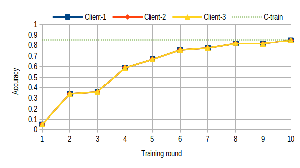
(a) Full-aggregation learning

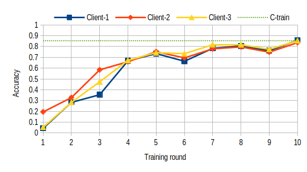
(b) Partly-aggregation learning

Figure 4. Accuracy of the secure federated learing. The dash-line (C-train) is the accuracy of the centralized learning.

Figure 4 shows that the performance of the local models is improved after 10 training rounds. For the Full-Aggregation Learning (Figure 4-a), the performance of all clients are similar, and their accuracy can reach 84.96% comparing to the accuracy of 85.4% in the Centralized Learning. Although the increment of accuracy is a bit different among clients in the Partly-Aggregation Learning, they are getting more converged at the end of the training phase. Comparing to the Centralized Learning, the performance of Client-1 and Client-3 in Partly-Aggregation Learning is equal to or even better than the ones in the Centralized Learning. The results are also reported in Table 3.

		Accuracy ($\%$)
Centralized Learning		85.4
Full-Aggregation Learning		84.96
Partly-Aggregation Learning	Client-1	85.84
	Client-2	83.63
	Client-3	85.4

Table 3. Comparison of the centralized learning and the secure federated learning.

6.3. Secure Federated Learning on the inhomogeneous SCDGs

Since the computing power is different from devices, the features, e.g., SCDG, are extracted accrordingly. The training graphs are computed in different techniques among clients even though that they are SCDGs. In this work, we consider three types of SCDG, that are extracted from binaries by the three different strategies in Section 3, i.e., BFS, CBFS and CDFS, at three clients. Particularly, Client-1 implements BFS, Client-2 implements CBFS, and Client-3 implements CDFS. The data proportion is reported in Table 2. In the scheme, the clients have their own training set and test set. The training sets are used to train their models. Then, the test sets are used to evaluate the performance of the models. Similar to previous experiment, we first implement the Centralized Learning in the client’s side. Then, we compare this results to the secure learning approach with 2 aggregation cases.

1. For the Centralized Learning, the model is separately trained on its training set for each client in 20 epoches. Then, this model is evaluated on the client’s test set.

2. For the Secure Federated Learning, we implment two types of aggregations: Full-Aggregation Learning and Partly-Aggregation Learning (see Section 5.3). The secure training is applied to train the local model for 20 training rounds. In each training round, the client trains the local model on its training set, and then, it evaluates the updated model on its own test set.

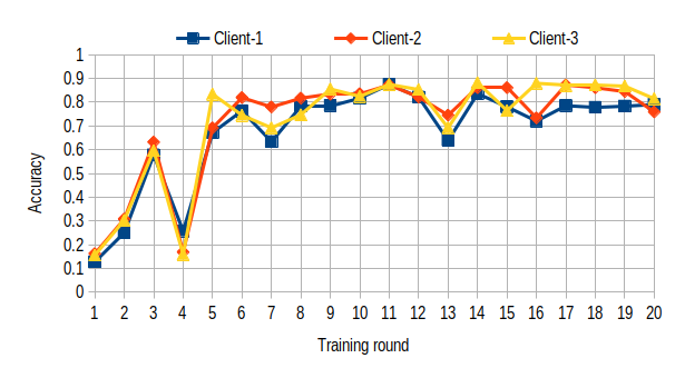
(a) Full-aggregation learning

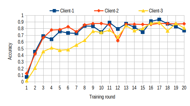
(b) Partly-aggregation learning

Figure 5. Accuracy of the secure federated learing in the inhomogeneous-data scheme.

		Accuracy ($\%$)
Centralized Learning	Client-1	92.05
	Client-2	81.02
	Client-3	89.9
Full-Aggregation Learning	Client-1	87.4
	Client-2	87.27
	Client-3	88.22
Partly-Aggregation Learning	Client-1	93.73
	Client-2	87.96
	Client-3	89.18

Table 4. Comparison of the centralized learning and the secure federated learning in the inhomogeneous-data scheme.

Figure 5-a shows that the performance of the local models is getting improvement after 20 training rounds in Full-Aggregation Learning. Three clients can reach the accuracy of $\sim 87\%$ after 11 training rounds. Then, the performance of Client-1 goes down to $79\%$ while Client-3 reach its peak, i.e., $88.22\%$, at the 14-th round. Compare to the Centralized Learning, Client-2 in Full-Aggregation Learning can achieve the better performance at the 8-th round. It reach 87.27% of accuracy, at the 11-th round while the accuracy in the Centralized Learning is 81.02%. The degradation at Client-1 in Full-Aggregation Learning is about $5.1\%$ comparing to the Centralized Learning. For Partly-Aggregation Learning in Figure 5-b, Client-1 gets the accuracy of 93.73% after 17 training rounds while Client-2 and Client-3 get 87.96% and 89.18%, respectively. The performance of Client-1 and Client-2 overtake the ones in Centralized Learning while the degradation at Client-3 is about 0.72%. The results are also reported in Table 4.

Overall, our secure learning approach is able to train the deep learning model for an accurate malware identifier. Comparing to the Centralized Learning, the performance gets a bit degradation in some client. It is a side-effect of calculation on the encrypted data in the secure aggregation. Besides, the experimental results also show that the Partly-Aggregation Learning overtakes the Full-Aggregation Learning in our system. Hence, the Partly-Aggregation Learning should be considered in the future implement of the federated learning for malware classification since it allows the clients collaborate with each other while keeping their classifier model in private.

7. Conclusion

In this paper, we present a deep learning model for malware classification and a secure learning approach to integrate this learning model into a feretated learning system. We validate the system to identify malwares on our datasets. We obtains a significant result with the accuracy of $\sim 85\%$. It is comparable to the Centralized learning. Moreover, we implement the system to learn SCDGs extracted from 3 various strategies. We can achieve the accuracy of $\sim 88\%$ in Full-Aggregation Learning and $\sim 93\%$ in Partly-Aggregation Learning, comparing to the accuracy of $\sim 92\%$ in Centralized Learning. According to the experimental results, the Partly-Aggregation Learning is a good option to employ a collaboratively learning for malware classification in future.

References

- (1)
- Abadi et al. (2016) Martin Abadi, Andy Chu, Ian Goodfellow, H Brendan McMahan, Ilya Mironov, Kunal Talwar, and Li Zhang. 2016. Deep learning with differential privacy. In Proceedings of the 2016 ACM SIGSAC conference on computer and communications security. 308–318.
- Aono et al. (2016) Yoshinori Aono, Takuya Hayashi, Le Trieu Phong, and Lihua Wang. 2016. Scalable and Secure Logistic Regression via Homomorphic Encryption. In Proceedings of the Sixth ACM Conference on Data and Application Security and Privacy (New Orleans, Louisiana, USA) (CODASPY ’16). Association for Computing Machinery, New York, NY, USA, 142–144. https://doi.org/10.1145/2857705.2857731
- Benaissa et al. (2021) Ayoub Benaissa, Bilal Retiat, Bogdan Cebere, and Alaa Eddine Belfedhal. 2021. TenSEAL: A Library for Encrypted Tensor Operations Using Homomorphic Encryption. arXiv:2104.03152 [cs.CR]
- Bertrand Van Ouytsel and Legay (2021) Charles-Henry Bertrand Van Ouytsel and Axel Legay. 2021. Detection and classification of malware based on symbolic execution and machine learning methods. In Cybersec & AI.
- Boenisch et al. (2021) Franziska Boenisch, Adam Dziedzic, Roei Schuster, Ali Shahin Shamsabadi, Ilia Shumailov, and Nicolas Papernot. 2021. When the Curious Abandon Honesty: Federated Learning Is Not Private. arXiv preprint arXiv:2112.02918 (2021).
- Burkhart et al. (2010) Martin Burkhart, Mario Strasser, Dilip Many, and Xenofontas Dimitropoulos. 2010. SEPIA: Privacy-Preserving Aggregation of Multi-Domain Network Events and Statistics. In Proceedings of the 19th USENIX Conference on Security (Washington, DC) (USENIX Security’10). USENIX Association, USA, 15.
- Chen et al. (2018) Yi-Ruei Chen, Amir Rezapour, and Wen-Guey Tzeng. 2018. Privacy-preserving ridge regression on distributed data. Information Sciences 451 (2018), 34–49.
- Chowdhary et al. (2021) Sangeeta Chowdhary, Wei Dai, Kim Laine, and Olli Saarikivi. 2021. EVA Improved: Compiler and Extension Library for CKKS. In Proceedings of the 9th on Workshop on Encrypted Computing & Applied Homomorphic Cryptography. 43–55.
- Dam et al. (2021) Khanh Huu The Dam, Thomas Given-Wilson, and Axel Legay. 2021. Unsupervised behavioural mining and clustering for malware family identification. In Proceedings of the 36th Annual ACM Symposium on Applied Computing. 374–383.
- Dam and Touili (2016) Khanh Huu The Dam and Tayssir Touili. 2016. Automatic extraction of malicious behaviors. In 2016 11th International Conference on Malicious and Unwanted Software (MALWARE). 1–10. https://doi.org/10.1109/MALWARE.2016.7888729
- Egele et al. (2008) Manuel Egele, Theodoor Scholte, Engin Kirda, and Christopher Kruegel. 2008. A survey on automated dynamic malware-analysis techniques and tools. ACM computing surveys (CSUR) 44, 2 (2008), 1–42.
- Fredrikson et al. (2010) Matt Fredrikson, Somesh Jha, Mihai Christodorescu, Reiner Sailer, and Xifeng Yan. 2010. Synthesizing near-optimal malware specifications from suspicious behaviors. In 2010 IEEE Symposium on Security and Privacy. IEEE, 45–60.
- Gálvez et al. (2020) Rafa Gálvez, Veelasha Moonsamy, and Claudia Diaz. 2020. Less is More: A privacy-respecting Android malware classifier using federated learning. arXiv preprint arXiv:2007.08319 (2020).
- Ghimire and Rawat (2022) Bimal Ghimire and Danda B Rawat. 2022. Recent Advances on Federated Learning for Cybersecurity and Cybersecurity for Federated Learning for Internet of Things. IEEE Internet of Things Journal (2022).
- Goodfellow et al. (2016) Ian Goodfellow, Yoshua Bengio, and Aaron Courville. 2016. Deep Learning. MIT Press. http://www.deeplearningbook.org.
- Gritti et al. (2020) Fabio Gritti, Lorenzo Fontana, Eric Gustafson, Fabio Pagani, Andrea Continella, Christopher Kruegel, and Giovanni Vigna. 2020. Symbion: Interleaving symbolic with concrete execution. In 2020 IEEE Conference on Communications and Network Security (CNS). IEEE, 1–10.
- Hsu et al. (2020) Ruei-Hau Hsu, Yi-Cheng Wang, Chun-I Fan, Bo Sun, Tao Ban, Takeshi Takahashi, Ting-Wei Wu, and Shang-Wei Kao. 2020. A Privacy-Preserving Federated Learning System for Android Malware Detection Based on Edge Computing. In 2020 15th Asia Joint Conference on Information Security (AsiaJCIS). 128–136. https://doi.org/10.1109/AsiaJCIS50894.2020.00031
- Kim et al. (2020) Andrey Kim, Antonis Papadimitriou, and Yuriy Polyakov. 2020. Approximate homomorphic encryption with reduced approximation error. Cryptology ePrint Archive (2020).
- Kingma and Ba (2014) Diederik P Kingma and Jimmy Ba. 2014. Adam: A method for stochastic optimization. arXiv preprint arXiv:1412.6980 (2014).
- Konečnỳ et al. (2016) Jakub Konečnỳ, H Brendan McMahan, Daniel Ramage, and Peter Richtárik. 2016. Federated optimization: Distributed machine learning for on-device intelligence. arXiv preprint arXiv:1610.02527 (2016).
- Lab (2021) Kaspersky Lab. 2021. Machine Learning Methods for Malware Detection. Retrieved 2022-02-24 from https://media.kaspersky.com/en/enterprise-security/Kaspersky-Lab-Whitepaper-Machine-Learning.pdf
- Lajevardi et al. (2021) Amir Mohammadzade Lajevardi, Saeed Parsa, and Mohammad Javad Amiri. 2021. Markhor: malware detection using fuzzy similarity of system call dependency sequences. Journal of Computer Virology and Hacking Techniques (2021), 1–10.
- Li et al. (2021) Beibei Li, Yuhao Wu, Jiarui Song, Rongxing Lu, Tao Li, and Liang Zhao. 2021. DeepFed: Federated Deep Learning for Intrusion Detection in Industrial Cyber–Physical Systems. IEEE Transactions on Industrial Informatics 17, 8 (2021), 5615–5624. https://doi.org/10.1109/TII.2020.3023430
- Li et al. (2018) He Li, Kaoru Ota, and Mianxiong Dong. 2018. Learning IoT in edge: Deep learning for the Internet of Things with edge computing. IEEE network 32, 1 (2018), 96–101.
- Lin and Huang (2020) Kuang-Yao Lin and Wei-Ren Huang. 2020. Using federated learning on malware classification. In 2020 22nd International Conference on Advanced Communication Technology (ICACT). IEEE, 585–589.
- Macedo and Touili (2013) Hugo Daniel Macedo and Tayssir Touili. 2013. Mining malware specifications through static reachability analysis. In European Symposium on Research in Computer Security. Springer, 517–535.
- Melis et al. (2019) Luca Melis, Congzheng Song, Emiliano De Cristofaro, and Vitaly Shmatikov. 2019. Exploiting unintended feature leakage in collaborative learning. In 2019 IEEE Symposium on Security and Privacy (SP). IEEE, 691–706.
- Namani and Khan (2020) Naveen Namani and Arindam Khan. 2020. Symbolic execution based feature extraction for detection of malware. In 2020 5th International Conference on Computing, Communication and Security (ICCCS). 1–6. https://doi.org/10.1109/ICCCS49678.2020.9277493
- Nguyen et al. (2019) Thien Duc Nguyen, Samuel Marchal, Markus Miettinen, Hossein Fereidooni, N. Asokan, and Ahmad-Reza Sadeghi. 2019. DÏoT: A Federated Self-learning Anomaly Detection System for IoT. In 39th IEEE International Conference on Distributed Computing Systems, ICDCS 2019, Dallas, TX, USA, July 7-10, 2019. IEEE, 756–767. https://doi.org/10.1109/ICDCS.2019.00080
- Nikolaenko et al. (2013) Valeria Nikolaenko, Udi Weinsberg, Stratis Ioannidis, Marc Joye, Dan Boneh, and Nina Taft. 2013. Privacy-preserving ridge regression on hundreds of millions of records. In 2013 IEEE symposium on security and privacy. IEEE, 334–348.
- Payne and Kundu (2019) Joshua Payne and Ashish Kundu. 2019. Towards Deep Federated Defenses Against Malware in Cloud Ecosystems. In 2019 First IEEE International Conference on Trust, Privacy and Security in Intelligent Systems and Applications (TPS-ISA). 92–100. https://doi.org/10.1109/TPS-ISA48467.2019.00020
- Phong et al. (2018) Le Trieu Phong, Yoshinori Aono, Takuya Hayashi, Lihua Wang, and Shiho Moriai. 2018. Privacy-Preserving Deep Learning via Additively Homomorphic Encryption. IEEE Transactions on Information Forensics and Security 13, 5 (2018), 1333–1345. https://doi.org/10.1109/TIFS.2017.2787987
- Regev (2009) Oded Regev. 2009. On lattices, learning with errors, random linear codes, and cryptography. Journal of the ACM (JACM) 56, 6 (2009), 1–40.
- Rey et al. (2022a) Valerian Rey, Pedro Miguel Sánchez Sánchez, Alberto Huertas Celdrán, and Gérôme Bovet. 2022a. Federated learning for malware detection in iot devices. Computer Networks (2022), 108693.
- Rey et al. (2022b) Valerian Rey, Pedro Miguel Sánchez Sánchez, Alberto Huertas Celdrán, and Gérôme Bovet. 2022b. Federated learning for malware detection in IoT devices. Computer Networks 204 (Feb 2022), 108693. https://doi.org/10.1016/j.comnet.2021.108693
- Said et al. (2018) Najah Ben Said, Fabrizio Biondi, Vesselin Bontchev, Olivier Decourbe, Thomas Given-Wilson, Axel Legay, and Jean Quilbeuf. 2018. Detection of mirai by syntactic and behavioral analysis. In 2018 IEEE 29th International Symposium on Software Reliability Engineering (ISSRE). IEEE, 224–235.
- Sebastio et al. (2020) Stefano Sebastio, Eduard Baranov, Fabrizio Biondi, Olivier Decourbe, Thomas Given-Wilson, Axel Legay, Cassius Puodzius, and Jean Quilbeuf. 2020. Optimizing symbolic execution for malware behavior classification. Computers & Security 93 (2020), 101775. https://doi.org/10.1016/j.cose.2020.101775
- Shoshitaishvili et al. (2016) Yan Shoshitaishvili, Ruoyu Wang, Christopher Salls, Nick Stephens, Mario Polino, Andrew Dutcher, John Grosen, Siji Feng, Christophe Hauser, Christopher Kruegel, and Giovanni Vigna. 2016. SOK: (State of) The Art of War: Offensive Techniques in Binary Analysis. In 2016 IEEE Symposium on Security and Privacy (SP). 138–157. https://doi.org/10.1109/SP.2016.17
- Singh and Singh (2021) Jagsir Singh and Jaswinder Singh. 2021. A survey on machine learning-based malware detection in executable files. Journal of Systems Architecture 112 (2021), 101861.
- Wang et al. (2018) Zhibo Wang, Mengkai Song, Zhifei Zhang, Yang Song, Qian Wang, and Hairong Qi. 2018. Beyond Inferring Class Representatives: User-Level Privacy Leakage From Federated Learning. arXiv e-prints, Article arXiv:1812.00535 (Dec. 2018), arXiv:1812.00535 pages. arXiv:1812.00535 [cs.LG] https://ui.adsabs.harvard.edu/abs/2018arXiv181200535W
- Willems et al. (2007) Carsten Willems, Thorsten Holz, and Felix Freiling. 2007. Toward automated dynamic malware analysis using cwsandbox. IEEE Security & Privacy 5, 2 (2007), 32–39.
- Zhang et al. (2021) Tuo Zhang, Chaoyang He, Tianhao Ma, Mark Ma, and Salman Avestimehr. 2021. Federated Learning for Internet of Things: A Federated Learning Framework for On-device Anomaly Data Detection. (June 2021). arXiv:2106.07976 [cs.LG]
- Zhao et al. (2019) Ying Zhao, Junjun Chen, Di Wu, Jian Teng, and Shui Yu. 2019. Multi-Task Network Anomaly Detection Using Federated Learning. In Proceedings of the Tenth International Symposium on Information and Communication Technology (Hanoi, Ha Long Bay, Viet Nam) (SoICT 2019). Association for Computing Machinery, New York, NY, USA, 273–279. https://doi.org/10.1145/3368926.3369705
- Zhu et al. (2019) Ligeng Zhu, Zhijian Liu, and Song Han. 2019. Deep leakage from gradients. Advances in Neural Information Processing Systems 32 (2019).