Network Topology Optimization via Deep Reinforcement Learning

Abstract

Topology impacts important network performance metrics, including link utilization, throughput and latency, and is of central importance to network operators. However, due to the combinatorial nature of network topology, it is extremely difficult to obtain an optimal solution, especially since topology planning in networks also often comes with management-specific constraints. As a result, local optimization with hand-tuned heuristic methods from human experts are often adopted in practice. Yet, heuristic methods cannot cover the global topology design space while taking into account constraints, and cannot guarantee to find good solutions.

In this paper, we propose a novel deep reinforcement learning (DRL) algorithm, called Advantage Actor Critic-Graph Searching (A2C-GS), for network topology optimization. A2C-GS consists of three novel components, including a verifier to validate the correctness of a generated network topology, a graph neural network (GNN) to efficiently approximate topology rating, and a DRL actor layer to conduct a topology search. A2C-GS can efficiently search over large topology space and output topology with satisfying performance. We conduct a case study based on a real network scenario, and our experimental results demonstrate the superior performance of A2C-GS in terms of both efficiency and performance.

I Introduction

Due to the rapid development of communication technologies, more devices are connected to the Internet. As a result, the network scale keeps increasing and the network infrastructure is continuously upgraded, e.g., by adopting large-capacity fiber optic cables, to keep up with the need for better service quality. Since main network performance metrics, such as link utilization, throughput and latency, are heavily affected by the network structure, topology optimization has thus become a critical problem for network operators and has received much attention.

However, the network planning problem is very challenging. First, the topology problem is combinatorial in nature. Thus, it is often of high complexity, i.e., exponential in the number of links. Second, to conduct network topology optimization, there are technical issues caused by complex management-specific constraints (often nonlinear) in network topology optimization, due to operation requirements, e.g., in terms of the allowed fraction of changed links, overall modification costs, or network performance such as link utilization after optimization. Therefore, different approaches have been proposed for various network topology planning scenarios. For instance, [1] formulates the network planning problem as a mixed integer linear programming problem. [6] formulates the problem as a complex multi-objective optimization problem, and focuses on cost minimization. [5] considers multi-layer capacity planning with the objective of multi-layer recovery. [23] proposes an algorithm NeuroPlan to optimize network topology. [20] proposes an approximation algorithm for topology optimization. [7, 17, 18] develop heuristic methods. Yet, these algorithms are not guaranteed to achieve close-to-optimal performance, and can only be applied to specified scenarios. Moreover, existing methods typically incur high computational complexity, primarily due to the combinatorial nature of network topology planning. Therefore, to support the rapidly increasing demand of good network service quality, there is an urgent need to develop efficient topology optimization methods to support network capacity expansion and improve operating performance through efficient searching.

In this work, we propose a novel solution to solve the graph topology optimization problem utilizing deep reinforcement learning (DRL), which is called Advantage Actor Critic-Graph Search (A2C-GS). DRL has been demonstrated to achieve superior performance in many scenarios, e.g., designing molecular structures [22], sharing bike scheduling [15] and IP-fiber cross-layer scheduling in network [23], and has also found applications in social recommendation [3] and wireless communication [8]. A2C-GS builds on the generalization power of DRL and consists of three key novel components, namely, a topology verifier to validate the correctness of a generated network topology, a graph neural network (GNN) to efficiently approximate the topology rating, and an RL actor based on A2C [12] to conduct topology search.

There have been works developing DRL algorithms for solving combinatorial optimization problems, e.g., learning cuts for integer programming [19], learning branching strategies for mixed integer linear programming [2], vehicle routing problem [14], online computing offload [9], and TSP problem [10]. Our work distinguishes itself from these results in the following. First, A2C-GS adopts a GNN for learning complex objective functions of the combinatorial problem. This enables us to efficiently rate the goodness of topologies to facilitate searching. Second, A2C-GS introduces a novel action space compression to avoid searching over an overly-large space (exponential in network size). Third, A2C-GS contains a topology verifier, which efficiently testifies the found solution and generates data for training GNN.

The main contributions of our paper are as follows.

First, we formulate a general network topology optimization problem $\mathtt{NetTopoOpt}$, which takes into account topology adjustment feasibility, adjustment cost, and performance impact. $\mathtt{NetTopoOpt}$ provides a clear formulation for optimizing combinatorial network topology.

Second, we propose a general DRL-based scheme named Advantage Actor Critic-Graph Searching (A2C-GS), which consists of three key novel components, a topology verifier to validate the correctness of a generated network topology, a GNN to efficiently approximate the topology rating, and an A2C actor layer to conduct topology search. The novel design of A2C-GS allows us to efficiently search over an exponentially large topology space.

Third, we carry out a case study based on a real network scenario from China Mobile [13] and conduct extensive experiments. Our results demonstrate that A2C-GS outperforms existing heuristic search algorithms in both small action space, i.e., with $O(2^{20})$ actions, and large search space, i.e., with $O(10^{21})$ actions.

II Problem definition

In this section, we present the network topology optimization formulation. Our overall objective is to find an optimal network topology starting from a given initial structure, to optimize a given performance metric, subject to management-specific constraints on the adjustment. Below, we present the general framework, based on which we present our solution framework. In the experiment section, we will carry out a detailed implementation based on a concrete setting. Specifically, for a given network, we denote its topology structure as $G=(V,E)$, where $V=\{1,2,...,N\}$ is the set of all vertices and $E=\{(m,n),m,n\in V\}$ is the set of all edges in the network. We define the adjacent matrix $\bm{x}$ of the graph $G$ as a variable of the connectivity property, i.e., if $i$ and $j$ are connected, $(\bm{x})_{ij}=1$, else $(\bm{x})_{ij}=0$. We denote the adjacent matrix of the initial topology as $\bm{x}_{0}$. We sometimes write the set of edges $E$ as $E(\bm{x})$ to clearly indicate that the set of edges $E$ is a function of $\bm{x}$. Note that $\bm{x}$ can have $\frac{N(N-1)}{2}$ values in reality. Then, we consider the following general constrained network topology optimization problem, which we refer to as $\mathtt{NetTopoOpt}$:

$$(\mathtt{NetTopoOpt})\,\,\max: f(\bm{x})=U(\bm{x})+\gamma Cost(\bm{x},\bm{x}_{0}),$$ (1)

s.t. $$Dist(e)\leq D,\ \forall e\in E(\bm{x}),$$ (4)

$$Load(e)\leq L_{max},\ \forall e\in E(\bm{x}),$$

$$M(\bm{x})=True.$$

Here the first term $U(\bm{x})$ denotes the performance of the network under the topology, e.g., utilization of the network links. This term captures the performance aspect of the network topology and is introduced to allow network operators to specify service requirements. It is a nonlinear representation of the input and often involves complex computation in practical scenarios (see Section IV for a concrete case study). $Cost(\bm{x},\bm{x}_{0})$ is the cost of transforming the graph from the initial topology ${\bm{x}_{0}}$ to the target value $\bm{x}$. This cost is usually proportional to the difference of the links in ${\bm{x}_{0}}$ and $\bm{x}$, due to deletion of old links and installation of new links. $\gamma<0$ is a weight between performance and cost.

We now explain the constraints. In the first constraint (4), $Dist(e)$ denotes the distance of the end nodes of $e$. Constraint (4) concerns the distance feasibility of the network topology adjustment, in that for each link $(i,j)$ in the new graph, the two end nodes $v_{i}$ and $v_{j}$ need to be within connection distance $D$, e.g., due to fiber cable length in a wired network or due to the wireless radio connection range in a mobile network. The second constraint (4) is on the utilization of the network links. Here $Load(e)$ denotes the utilization of the link, and $L_{max}$ is the maximum allowed utilization level. In practice, there are often constraints on link utilization, e.g., $90\%$ [11]. The third condition (4) is an abstract feasibility requirement of the topology. Such a constraint is often due to network management requirements and allows operators to impose policy-based restrictions on the resulting network topology (similar to BGP [21] on routing). For instance, there can be a length constraint on any path between a pair of nodes.

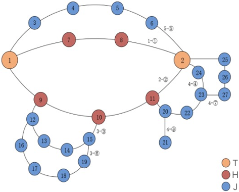
Fig. 1 below gives a concrete example of a network topology. In this example, there are three different types of nodes, denoted as type-$T$, type-$H$ and type-$J$, corresponding to nodes with different functionalities. The distance constraint (4) in this example means that any edge connecting two nodes is bounded by a maximum distance. The constraint (4) means that the aggregation of average traffic volume in type-$H$ nodes is no larger than the maximum utilization of type-$T$ nodes. Constraint (4) here requires that if a type-$J$ node and a type-$H$ node are connected, the maximum utilization, denoted by $U_{\max}(\cdot)$ (see Section IV), of the type-$J$ node is no larger than that of the type-$H$ node for workload balance, e.g., $U_{\max}(12)\leq U_{\max}(9)$.

Figure 1: An example of a network topology. There are different node types and the formation of the network is constrained by the management requirements.

Note that our $\mathtt{NetTopoOpt}$ problem (1) is general and offers a framework for network topology optimization. However, from the definition and description of constraints, we see that the problem involves a complex combinatorial objective function and nonlinear constraints. As a result, existing heuristic optimization algorithms mostly lead to sub-optimal solutions. Besides, exact search algorithms will incur large computation complexity. Therefore, there is a strong need to design efficient algorithms. Below, we describe our novel deep reinforcement learning based method. Our method builds upon the generalization power of neural networks and introduces techniques for handling the heavy computation requirement due to complex network structure.

III Methods and algorithms

In this section, we present our DRL based algorithm, called Advantage Actor Critic-Graph Searching (A2C-GS). The procedure of A2C-GS is shown in Fig. 2 below. Specifically, A2C-GS contains a representation component, a DRL agent, and a topology verifier. The representation component learns the network objective function and compresses the action and state spaces. It is introduced to reduce computation complexity due to large search space, i.e., $O(2^{\frac{|V|(|V|-1)}{2}})$ combinations, which makes even verifying the correctness of a topology difficult. The DRL agent is used to learn control actions based on reinforcement learning updates based on the A2C algorithm [12] and works with the state, action and reward. The topology verifier is introduced to check feasibility of the output topology, so as to ensure with certainty that all constraints from network operators are guaranteed. It can also be used to help data generation in the large network setting (see Section IV for a concrete case study).

Figure 2: The procedure of A2C-GS. There are three main components, representation layer, DRL agent and verifier. Here $s$ denotes a state, $a$ denotes an action, $r$ denotes a reward function. $T(s,a)$ denotes the transition function. $\pi_{\theta}$ denotes a parameterized policy. $f(s)$ is the objective value calculated by the verifier. A2C-GS utilizes the representation layer to compress the state and action to $s_{0}$ and $a_{0}$ and the GNN classifier $\tilde{f}$ to learn the true objective function $f$.

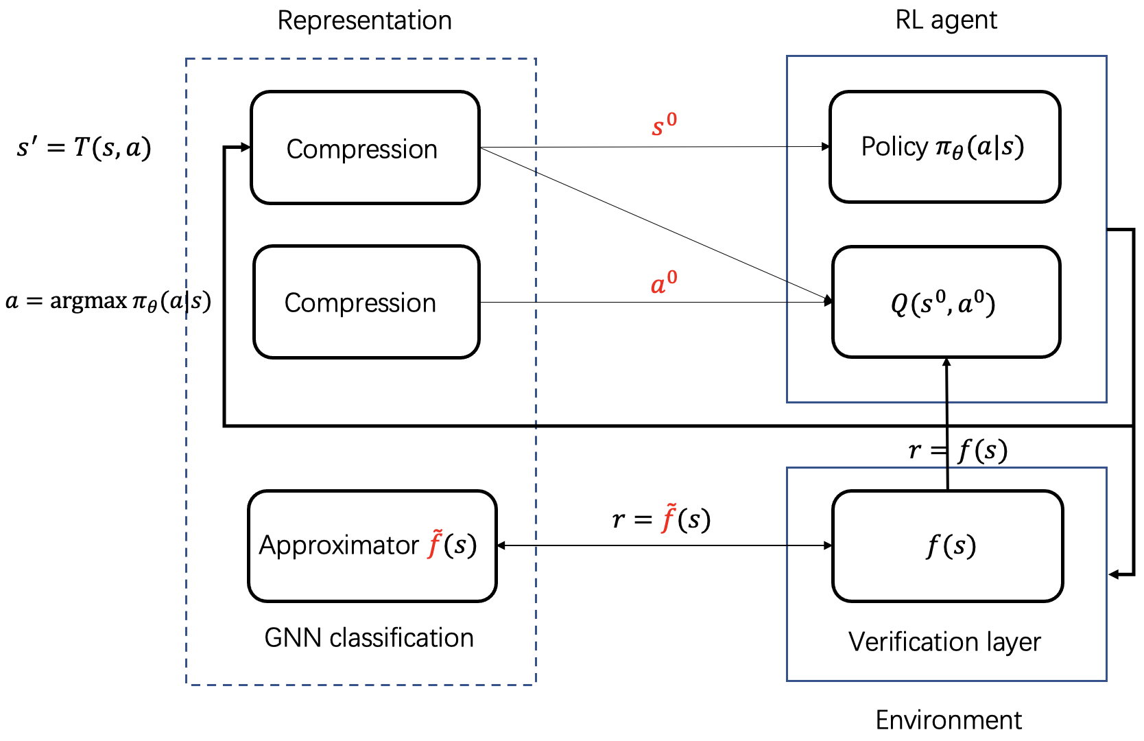
Below, we explain A2C-GS in detail. We denote the initial state space as $S=\{\bm{x}=(x_{ij}:i,j\in V):\bm{x}\,\,\text{feasible}\}$ (following the tradition, we will also use $s$ to denote a state when it is clear) and the action space as $A=\{a=(a_{ij}:i,j\in V):a\,\,\text{feasible}\}$. The next state is defined by the action and transition method $T(\cdot)$ that $x_{ij}(t+1)=T(x_{ij}(t),a_{ij})=x_{ij}(t)+a_{ij}\ (\text{mod}\ 2)$.

The formal procedure of A2C-GS is shown in Algorithm 1. A2C-GS makes use of a verification oracle $\mathtt{Verifier}$ (shown in Algorithm 2) to verify whether an output topology is valid and compute the objective value. In Section IV, we will show a concrete verifier algorithm based on specified network management requirements. A2C-GS also provides an optimization method for training RL agents, and provide the $\mathtt{GNNTraining}/\mathtt{GNNTesting}$ algorithm for a classifier and action space choice for representation.

Step 2 initializes the value to choose the GNN or $\mathtt{Verifier}$ algorithm. Step 3 chooses the action space. Choosing the compressed action space enables an efficient search over the state space. Step 5 trains the RL agent using the A2C algorithms [12]. During training, if we use the $\mathtt{Verifier}$ algorithm to directly calculate the objective value as the reward, i.e., $C_{f}=1$, we collect the data in the replay buffer for training GNN. Otherwise, i.e., $C_{f}=2$, we use $0$ or $1$ (label poor or good graph) as the reward. This is done to further reduce the complexity in providing detail rating, which can still face high computational complexity. Step 6 is the process of GNN training (Algorithm 3). Step 7 generates data by the agent and invokes the $\mathtt{Verifier}$ to test the topology. Step 8 is the procedure of testing GNN (Algorithm 4). Since data from Step 7 are not used in training GNN, they are used as testing data to examine the performance of a GNN classifier.

1:  Input: Initial graph $G=(V,E)$, a GNN $\tilde{f}_{\phi(t)}$ with parameter $\phi(t)$, policy $\pi_{\theta}(a|s)$, replay buffer $\mathcal{B}$, timestep number $H$, epoch number $m$, threshold value $q$.

2:  Initialize GNN $\tilde{f}_{\phi(1)}$ and policy $\pi_{\theta}(a|s)$. Set reward calculation choice $C_{f}=1$ ($1$ means reward obtained from $\mathtt{Verifier}$, $C_{f}=2$ means it is obtained from GNN)

3:  Choose the state and action choice $C_{a}$ ($1$ means full space, $2$ means compressed space).

4:  for epoch $i=1,...,m$ do

5:     Run A2C algorithm for $H$ steps with choice $C_{f}$ and $C_{a}$, compute the policy gradient and update the parameter $\theta$. If $C_{f}=1$, collect data $\{a^{j},s^{j},r^{j}\}_{j=1}^{H}$ into replay buffer $\mathcal{B}$.

6:     Run $\mathtt{GNNTraining}$ (Algorithm 4) to train GNN. Input $\tilde{f}_{\phi(t)}$, data in $\mathcal{B}$, threshold value $q$, and output $\tilde{f}_{\phi(t+1)}$.

7:     Generate an action sequence $\{a_{1},a_{2},...a_{n}\}$ and the corresponding topologies $\{s_{1},s_{2},...s_{n}\}$ using the policy $\pi_{\theta}$. Run $\mathtt{Verifier}$ to validate the graphs and compute the objective values $\{r_{1},r_{2},...r_{n}\}$, and add the data to replay buffer $\mathcal{B}$.

8:     Run $\mathtt{GNNTesting}$ (Algorithm 3) with input $\tilde{f}_{\phi(t)}$ and data generated by step 7 and output $P(\tilde{f}_{\phi(t)})$. If $P(\tilde{f}_{\phi(t)})<95\%$, $C_{f}=1$, else $C_{f}=2$.

9:  end for

Algorithm 1 A2C graph search algorithm (A2C-GS)

1:  Input: the initial graph $G(\bm{x_{0}})=(V,E(\bm{x_{0}}))$ with adjacent matrix $\bm{x_{0}}$, the target graph $G(\bm{x})=(V,E(\bm{x}))$.

2:  For every edge $e\in\tilde{E}$, if $Dist(e)>D$, return invalid. (Distance requirements)

3:  For every edge $e\in\tilde{E}$, if $Load(e)>L_{\max}$, return invalid. (Utility requirements)

4:  If the graph $G(\bm{x})$ is such that $M(\bm{x})=False$, return invalid. (Feasibility requirements)

5:  If these requirements are satisfied, return valid and compute the objective value by the formation: $f(\bm{x})=U(\bm{x})+\gamma Cost(\bm{x},\bm{x}_{0})$. (Objective computation)

Algorithm 2 General $\mathtt{Verifier}$ algorithm

1:  Input: GNN layer parameter as function $\tilde{f}_{\phi(t)}$, replay buffer $\mathcal{B}$, threshold value $q$.

2:  for Epoch $\tau=1,...,T$ do

3:     Shuffle replay buffer $\mathcal{B}$ and collect $n$ pairs of data $D=\{(s_{i},r_{i})\}_{i=1}^{n}$. Label graph data as $\{(s_{i},\tilde{r}_{i})\}_{i=1}^{n}$. $\forall(s_{i},r_{i})\in D$, if $r_{i}\geq q,\tilde{r}_{i}=1$, else $\tilde{r}_{i}=0$.

4:     For every $d_{i}=(s_{i},r_{i})\in D$, update the function parameter $\phi(t)$ by optimizer.

5:  end for

6:  Return New GNN layer parameter $\phi(t+1)\leftarrow\phi(t)$

Algorithm 3 $\mathtt{GNNTraining}$ algorithm

1:  Input: Data $D=\{s^{j},r^{j}\}_{j=1}^{H}$, GNN $\tilde{f}_{\phi(t)}$, threshold value $q$.

2:  Label graph data as $\{(s_{j},\tilde{r}_{j})\}_{j=1}^{H}$. $\forall(s_{j},r_{j})\in D$, if $r_{j}\geq q,\tilde{r}_{j}=1$, else $\tilde{r}_{j}=0$.

3:  Return $P(\tilde{f}_{\phi(t)})=\sum_{j=1}^{H}\mathbb{I}(\tilde{f}_{\phi(t)}(s_{j})=\tilde{r}_{j})/H$

Algorithm 4 $\mathtt{GNNTesting}$ algorithm

IV Case Study and Experiments

IV-A The concrete topology optimization problem

In this section, we present a concrete case study, which is based on a real-world network management scenario from China Mobile [13] with the topology and traffic volume information of a specific city. Below, we will present the background description, problem definition, constraints and concrete A2C-GS implementation. Table I summarizes the key notations. In the case study, we use two datasets, the small dataset and the large dataset. In the small dataset, we use simulated location information to demonstrate the efficiency of compressing action space. In the large dataset, all node locations are obtained from the real dataset. In both datasets, all network-related information, including node type, maximum utilization and average traffic volume, are from the China Mobile dataset.

We consider a link load balancing problem in the optical communication process at the bottom of the transmission network between network elements, i.e., nodes. The objective is to optimize the topology structure from an initial topology, to achieve balance. Now we specify the details of the $\mathtt{NetTopoOpt}$ formulation for the case study, including the objective function and constraints.

TABLE I: Basic definitions of node features in the graph

Symbol	Description
$Type(v)$	There are three node types, $T$, $H$ and $J$, representing nodes in core layer, aggregation
	layer and access layer, respectively
$U_{\max}(v)$	Maximum utilization of node $v$ with Gbps unit, representing maximum processing bandwidth of a node
$Pos(v)$	Position of node $v$, i.e., the longitude and magnitude
$Flow(v,t)$	Average traffic volume passing through node $v$ per hour with Mbps unit

IV-A1 Objective function

Recall that the objective function is $f(\bm{x})=U(\bm{x})+\gamma Cost(\bm{x},{\bm{x_{0}}})$, where $\bm{x}$ is the adjacent matrix of $G$, and $\bm{x_{0}}$ is its initial value. First, $Cost(\bm{x},{\bm{x_{0}}})$ is defined as

$$Cost(\bm{x},{\bm{x_{0}}})=\sum_{i,j}\left(\lambda_{0}Dist(v_{i},v_{j})\mathbb{I}((\bm{x_{0}})_{ij}=0)+\lambda_{1}\mathbb{I}((\bm{x_{0}})_{ij}=1)\right)|(\bm{x})_{ij}-(\bm{x_{0}})_{ij}|,$$ (5)

where $Dist(v_{i},v_{j})$ is the distance between two nodes $v_{i}$ and $v_{j}$; $\mathbb{I}(\mathcal{E})$ is the indicator function of event $\mathcal{E}$, i.e., it is one if $\mathcal{E}$ is true. $\lambda_{0}$ and $\lambda_{1}$ are constant parameters. This means that if an initial edge is not adapted, it does not influence the cost. If an edge is newly built, the cost is related to the distance. If an edge is removed, the cost is constant.

Next, we specify $U(\bm{x})$. Specifically, in the graph $G$, there exists a path set denoted by $\mathcal{P}=\{1,2,...,P\}$, which consists of a set of $P$ paths described in Table II.

TABLE II: Definition of the notations for formation requirements

Notations	Definitions
Primary main path	The two end nodes of the path are both type-$T$ nodes and the intermediate nodes are type-$H$
Secondary main path	The two end nodes of the path are either $T$ or $H$, and the intermediate nodes are of type-$J$
Main path	Primary main path and secondary main path.
Sub path	When there are multiple candidate secondary main paths share the same two end nodes, one
	of them will be declared the secondary main path (see Algorithm 6), and the others will be
	called sub paths.
Path	Main path and sub path
Hang node	Nodes with degree $1$ and connect to an intermediate node in a path.

For each $p\in\mathcal{P}$, $Flow(p,t)$ denotes its bandwidth utilization at time $t$. Then, the utility value $U(\bm{x})$ of a graph is defined as:

$$\begin{split}U(\bm{x})=&\frac{1}{24P}\sum_{p\in\mathcal{P}}\sum_{t=1}^{24}\mathbb{I}\left(\left|\frac{Flow(p,t)}{B(t)}-1\right|\leq\epsilon\right)-\frac{1}{P}\sum_{p\in\mathcal{P}}(\alpha Sratio(p)+\beta Hratio(p))\\ &-\frac{1}{24}\sum_{t=1}^{24}Flow(\mathcal{P},t)-\max_{t}Flow(\mathcal{P},t)-\min_{t}Flow(\mathcal{P},t),\end{split}$$ (6)

where $Flow(\mathcal{P},t)=\frac{1}{P}\sum_{p\in\mathcal{P}}\left(Flow(p,t)-\frac{1}{P}\sum_{p\in\mathcal{P}}Flow(p,t)\right)^{2}$. $Sratio(p)$ is the percentage of nodes in a sub path for a path, $Hratio(p)$ is the percentage of nodes with degree $1$ in graph $G$ for a path. $B(t)$ is the benchmark bandwidth utilization in time $t$, which is the average bandwidth utilization of paths in the initial graph, and $\epsilon$ is the constant threshold value.

The first term $\frac{1}{24P}\sum_{p\in\mathcal{P}}\sum_{t=1}^{24}\mathbb{I}\left(\left|\frac{Flow(p,t)}{B(t)}-1\right|\leq\epsilon\right)$ is the average of the indicator value for all links and times. It means that if the bandwidth utilization $Flow(p,t)$ for a path is close to the benchmark $B(t)$, it helps the balance of path load. The second term $\frac{1}{P}\sum_{p\in\mathcal{P}}(Sratio(p)+Hratio(p))$ means that the value of sub ratio and hang ratio of a path cannot be too large. The last three terms represent the difference in bandwidth utilization among paths. In the case study, the values are set to be $\epsilon=0.4,\alpha=0.02,\beta=0.05,\lambda_{0}=10^{-8},\lambda_{1}=10^{-10},\gamma=-10^{-3}$.

IV-A2 Topology formation requirements

Here we present the concrete constraints on network topology, i.e., (4) to (4) in $\mathtt{NetTopoOpt}$, for the case study.

The distance requirement: The network requires that for any link $e=(i,j)$, $Dist(e)\leq D$, where $Dist(e)$ is the length of the link, and $D$ is the maximum allowed distance.

The utility requirement: For any path $p\in\mathcal{P}$, $Flow(p,t)\leq 1$, where $1$ is the maximum capacity value of a path. Notation $Flow(p,t)$ replaces $Load(e)$ described in Section II in the case study and we examine $Flow(p,t)$ to state whether or not a graph satisfies utility requirement.

The feasibility requirement: The graph $G$ needs to be a connected graph, which guarantees the connectivity of any two nodes. For any path $p\in\mathcal{P}$, the number of nodes in path $p$ cannot exceed $15$. For a path $p$, we denote the two end nodes, by $v_{h}$ and $v_{t}$. For other nodes $v\in p$, the maximum utilization value of node $v$, denoted as $U_{\max}(v)$, cannot be larger than the maximum value of the end nodes, i.e., $U_{\max}(v)\leq\max\{U_{\max}(v_{h}),U_{\max}(v_{t})\}$. There can also be nodes that connect to intermediate nodes in a path and has a degree $1$. We call such nodes hang nodes. Then, for a hang node $v_{H}$ attached to another node $v_{A}$, $U_{\max}(v_{H})\leq U_{\max}(v_{A})$. These requirements prevent overloading in a path.

IV-B A2C-GS for topology search

For optimizing the topology, we use the A2C-GS algorithm as a search method. Recall that the A2C-GS algorithm consists of two main parts: the verification part to validate whether or not a graph can calculate the objective value, and the optimization part by using RL algorithm to search graphs for optimizing the function. We specify the steps of A2C-GS in this case.

IV-B1 The $\mathtt{Verifier}$ Algorithm

First, given a graph, we need to know its validation. Based on constraints (4) to (4), we construct the topology validation method $\mathtt{Verifier}$ shown in Algorithm 5, which determines whether a generated topology is validated and calculates its objective value. If a graph is invalid, the algorithm returns false and a low objective value (set to $-10$ in our implementation). Otherwise, it returns true and the objective value. In Algorithm 5, $N(p)$ is the number of nodes in path $p$. $Head(p)$ and $Tail(p)$ are the end nodes of a path. $Dist(e)$ is the distance of an edge $e$. $Deg(v)$ is the degree of a node $v$ in graph $G$. $Nbr(v)$ denotes the set of neighbor nodes of node $v$ in $G$.

1:  Input: Graph $G=(V,E)$ and features of a node: $U_{\max}(V)$, $Pos(V)$, $Type(V)$.

2:  $\forall e\in E$, if $Dist(e)>500$, return invalid.

3:  Generate a subgraph $G^{\prime}=(V^{\prime},E^{\prime})\subset G$ that $\forall v^{\prime}\in V^{\prime},Type(v^{\prime})=T/H$. $\forall v\in V^{\prime}$, if $Type(v)=H$ and $Deg(v)\neq 2$ in $G^{\prime}$, return invalid. Run $\mathtt{BFS}$ algorithm for $G^{\prime}$ to search all primary main paths $\mathcal{P}_{P}=\{p_{P}^{(i)}\}_{i=1}^{m}$ between nodes $v\in V^{\prime}$ that $Type(v)=T$.

4:  Generate a subgraph $G^{\prime\prime}=(V^{\prime\prime},E^{\prime\prime})$, $V^{\prime\prime}=V$, and $\forall e^{\prime\prime}\in E^{\prime\prime},p_{P}^{(i)}\in\mathcal{P}_{P},e^{\prime\prime}\notin p_{P}^{(i)}$. Run $\mathtt{BFS}$ algorithm for $G^{\prime\prime}$ to search all possible secondary main paths $\mathcal{P}_{S}=\{p_{S}^{(i)}\}_{i=1}^{n}$ between nodes $v\in V^{\prime\prime}$ that $Type(v)=T/H$.

5:  Run $\mathtt{SelectBestPath}$ (Algorithm 6). If the output is invalid value -1, return invalid. Else the output is $\mathcal{P}_{S}^{0}=\{p_{S}^{(i)}\}_{i=1}^{n_{0}}\subset\mathcal{P}_{S}$ as secondary main path set and $\mathcal{P}_{S}^{1}=\{p_{S}^{(j)}\}_{j=1}^{n_{1}}\subset\mathcal{P}_{S}$ as the sub path set with attached relationship $\mathcal{RL}=\{(p_{S}^{(i)},p_{S}^{(j)})\},p_{S}^{(i)}\in\mathcal{P}_{S}^{0},p_{S}^{(j)}\in\mathcal{P}_{S}^{1}$.

6:  $\forall t,p\in\mathcal{P}_{S}\cup\mathcal{P}_{P}$, if $\sum_{v\in p}Flow(v,t)>\max\{U_{\max}(Head(p)),U_{\max}(Tail(p))\}$, return invalid.

7:  $\forall p\in\mathcal{P}_{S}\cup\mathcal{P}_{P}$, if $\exists v\in p,U_{\max}(v)>\max\{U_{\max}(Head(p)),U_{\max}(Tail(p))\}$, return invalid. $\forall p\in\mathcal{P}_{S}^{0}\cup\mathcal{P}_{P}$, if $N(p)>15$, return invalid. $\forall v\in V$, if $Deg(v)=0$ in $G$, return invalid. $\forall v_{1}\in V$, $Deg(v_{1})=1$ in $G$, for $v_{2}\in Nbr(v_{1})$, if $U_{\max}(v_{2})<U_{\max}(v_{1})$, return invalid.

8:  If these conditions are satisfied, return valid graph and run $\mathtt{CalObjValue}$ (Algorithm 7) to calculate the objective value for a graph.

Algorithm 5 The $\mathtt{Verifier}$ algorithm

Step 2 is the distance constraints to control the maximum distance for two connected nodes. Step 6 is the utility constraints. The other steps are the feasibility requirements. Step 3 ensures that the degree of type-$H$ node is $2$ in the subgraph. Step 5 means that the secondary main path satisfies the requirements executed in the $\mathtt{SelectBestPath}$ algorithm. Step 7 checks that the number of nodes in the main path and the maximum utilization value of the intermediate nodes is no larger than the end nodes. Besides, this step checks the connectivity in graph $G$ and the maximum utilization of the hang node is no larger than that of the connected node.

In order to verify the feasibility and compute the objective value, in Steps 3 and 4, we run breadth-first search algorithm ($\mathtt{BFS}$) to search all possible connected paths between two nodes. However, we cannot determine which is the secondary main path if there are many candidates. The $\mathtt{SelectBestLink}$ algorithm (Algorithm 6) helps the determination. The overall verification steps help determine whether or not a graph is valid. If any of the steps is violated, the algorithm returns invalid with a large negative value. If the graph is valid, we run the $\mathtt{CalObjValue}$ algorithm to compute the objective value as described in Algorithm 7.

Take Fig. 1 as an example. The distance of the edge between node $1$ and node $7$ cannot be larger than $500$m. Consider a path $p=\{1-7-8-2\}$, $Flow(p,t)$ is bounded by the maximization utility $1$. The feasibility requirements are as follows. The graph need to be connected. Any path cannot contain more than $15$ nodes. For instance, a path $p=\{1-7-8-2\}$ has $4$ nodes, which satisfies the requirement. For the path $p=\{1-7-8-2\}$, the maximum utilization value of nodes $7$ and $8$ cannot be larger than those of nodes $1$ and $2$ (the end nodes). The maximum utilization value of node $21$ cannot be larger than that of node $20$.

1:  Input: All possible secondary main paths $\mathcal{P}_{S}=\{p_{S}^{(i)}\}_{i=1}^{n}$

2:  Initialize: Set a Head-tail node buffer $\mathcal{H}$, a secondary main path $\mathcal{P}_{S}^{0}$, a sub path $\mathcal{P}_{S}^{1}$ and an attached relationship buffer $\mathcal{RL}$

3:  For all paths $p_{S}^{(i)}\in\mathcal{P}_{S}$, add the $\{Head(p_{S}^{(i)}),Tail(p_{S}^{(i)})\}$ set into the buffer $\mathcal{H}$. Set a buffer $P_{S}(\{Head(p_{S}^{(i)}),Tail(p_{S}^{(i)})\})$ and add $p_{S}^{(i)}$ into the buffer.

4:  For every path $p_{S}^{(i)}$ in the buffer $\mathcal{P}_{S}(\{Head(p_{S}^{(i)}),Tail(p_{S}^{(i)})\})$, if $\exists v_{i},v_{j}\in p_{S}^{(i)}$ that $Type(v_{i})=Type(v_{j})=J,U_{\max}(v_{i})\neq U_{\max}(v_{j})$, add $p_{S}^{(i)}$ into buffer $\mathcal{P}_{S}^{1}$.

5:  If all paths $p_{S}^{(i)}$ in the buffer $\mathcal{P}_{S}(\{Head(p_{S}^{(i)}),Tail(p_{S}^{(i)})\})$ belong to $\mathcal{P}_{S}^{1}$, return an invalid value -1. If there exist some paths not in $\mathcal{P}_{S}^{1}$, for these paths, find one path $p_{S}^{(i)}$ that maximizes $N(p_{S}^{(i)})$ and add to $\mathcal{P}_{S}^{0}$. Add other paths to $\mathcal{P}_{S}^{1}$ and add $(p_{S}^{(i)},p_{S}^{(j)})$ to $\mathcal{RL}$.

6:  Return a secondary main path $\mathcal{P}_{S}^{0}$, a sub path $\mathcal{P}_{S}^{1}$ and an attached relationship buffer $\mathcal{RL}$

Algorithm 6 $\mathtt{SelectBestPath}$ algorithm

1:  Input: The primary main path set $\mathcal{P}_{P}=\{p_{P}^{(i)}\}_{i=1}^{m}$, secondary main path $\mathcal{P}_{S}^{0}=\{p_{S}^{(i)}\}_{i=1}^{n_{0}}$, sub path set $\mathcal{P}_{S}^{1}=\{p_{S}^{(j)}\}_{j=1}^{n_{1}}$, the attached relationship $\{(p_{S}^{(i)},p_{S}^{(j)})\},p_{S}^{(i)}\in\mathcal{P}_{S}^{0},p_{S}^{(j)}\in\mathcal{P}_{S}^{1}$. Benchmark $B(t)$. The graph $G$ that generates the paths.

2:  For every secondary main path $p_{S}^{(i)}\in\mathcal{P}_{S}^{0}$, set that $Snumber(p_{S}^{(i)})=0$ as the number of nodes in sub path. Store $Head(p_{S}^{(i)})$ and $Tail(p_{S}^{(i)})$.

3:  For every sub path $p_{S}^{(j)}\in\mathcal{P}_{S}^{1}$, find the corresponding secondary main path $p_{S}^{(i)}\in\mathcal{P}_{S}^{0}$, set $Snumber(p_{S}^{(i)})\leftarrow Snumber(p_{S}^{(i)})+N(p_{S}^{(i)}\cup p_{S}^{(j)})-N(p_{S}^{(i)}),p_{S}^{(i)}\leftarrow p_{S}^{(i)}\cup p_{S}^{(j)}$.

4:  For every main path $p\in\mathcal{P}_{S}^{0}\cup\mathcal{P}_{P}$, $Flow(p,t)=\frac{\sum_{v\in p\backslash\{Head(p),Tail(p)\}}Flow(v,t)}{\max\{U_{\max}(Head(p)),U_{\max}(Tail(p))\}}$ , and for every node $v\in p$, the degree of the node in graph $G$ is $Deg(v)$, calculate $Hratio(p)=\frac{\sum_{v\in p}\mathbb{I}(Deg(v)=1)}{N(p)}$. For every secondary main path $p_{S}^{(i)}\in\mathcal{P}_{S}^{0}$, $Sratio(p_{S}^{(i)})=\frac{Snumber(p_{S}^{(i)})}{N(p_{S}^{(i)})}$

5:  Calculate $U(\bm{x})$ and $Cost(\bm{x},\bm{x_{0}})$ as the definitions and return $f(\bm{x})$.

Algorithm 7 $\mathtt{CalObjValue}$ algorithm

IV-B2 Action Compression in A2C-GS

Although DRL enables efficient search, it still suffers from the curse of dimensionality when facing problems with high-dimensional action spaces. Consider a network topology in our case with $23$ nodes and $72$ valid edges. This leads to an action space with $4.7\times 10^{21}$ option if we use a brute force enumeration, which is almost impossible to search over. To solve this problem, we propose a compact definition of the action space in our RL algorithm. Specifically, we define a compact action consisting of five steps, each corresponding to a decision at a particular level (see below), which will significantly improves the search efficiency of the algorithm. Before introducing the steps, we give some basic definitions first. We generate a connected graph $G^{*}=(V,E^{*})$ that we connect all edges satisfying $Dist(e)\leq D$. Based on the graph $G^{*}$, we generate subgraphs $G_{1}$ and $G_{2}$. $G_{1}$ consists of all type-$H$ nodes and all links connecting type-$H$ nodes in graph $G^{*}$. $G_{2}$ is alike $G_{1}$ with type-$J$ nodes format. We run the $\mathtt{BFS}$ algorithm for the subgraph $G_{1}$ and $G_{2}$ to generate all connection components regarded as basic components preparing for generating new components. Based on these components, we define our five-step action as below. Fig. 3 shows how to utilize these steps to generate a graph.

Figure 3: Schematic diagram of action compression into five steps.

Step 1. The first step decides how many sub-components to have from a basic component. For example, we can divide a basic component consisting of $6$ nodes into $2$ sub-components in Fig. 3.

Step 2. The second step decides how many nodes to assign to each sub-component. For example, consider the $2$ sub-components obtained from the first step in Fig. 3. There are $3$ potential choices to assign nodes, i.e., $\{(5,1),(4,2),(3,3)\}$. Specifically, $(5,1)$ means that one sub-component has $5$ nodes and the other sub-component has $1$ node.

Step 3. The third step decides the allocation of nodes for each sub-component. Consider the example as above that selects $(4,2)$ for node assignment, there are $15$ choices to allocate $6$ different nodes into two sub-components. Note that the first three steps influence the objective value, by affecting the bandwidth utilization of a path.

Step 4. The fourth step connects the nodes in the sub-components to make each sub-component fully connected. Take a sub-component with $4$ nodes in Fig. 3 as an example, there are at least $3$ edges in it. Consider the management requirements, the number of choices is less than $2^{\frac{4\times 3}{2}}=64$. This step influences the objective value by determining the sub ratio and hang ratio of a path.

Step 5. In the fifth step, we connect all the sub-components according to the management requirements to form one connected component. We especially consider connecting two sub-components that one is all type-$H$ nodes and another is all type-$J$ nodes. The number of potential choices is determined by the number of components and nodes in each component and the management requirements. The step influences the objective value by determining the maximum utilization of the end nodes in a path to influence the bandwidth utilization.

By using the above five-step action, we obtain a compact action space compared to working on modifying each link. However, the resulting action space is still very large. For instance, a graph has only one component with $16$ nodes initially. In the first step, we decide to divide the component into $4$ sub-components. In the second step, we decide that every sub-component has $4$ nodes. Based on the first and second steps, the third step has $2.6$ million potential choices (the number of possible ways to allocate $16$ different nodes evenly into $4$ components is $16!/(4!)^{5}$) while the fourth step has $2.1$ million potential choices (for each component with $4$ nodes, the number of all possible choices for connecting the component is $38$, and for all components the number is $38^{4}$). It is impossible for the RL agent to train a policy in this situation.

To further tackle the curse of dimensionality, in actual implementation, we further reduce the action space by imposing restriction on the choices in different steps, based on prior knowledge of the setting. Specifically, if there are too many choices in a step, we restrict ourselves to a pre-specified option set. The elements in the step set are chosen according to prior knowledge such that the size of the step set is neither too large nor too small, to enable efficient decision making. Although this restriction may limit possible actions, it is effective in reducing the size of the action space and allows for higher learning efficiency.

IV-B3 Reward function representation

To enable efficient search, we introduce a graph neural network (GNN) to facilitate reward learning. The motivation is that in large networks, the $\mathtt{Verifier}$ algorithm is time-consuming, while GNN can classify a good graph efficiently. The reason is that GNN contains nonlinear components to extract the feature and generate the discrimination directly, while $\mathtt{Verifier}$ algorithm judges the validation and calculate the objective value by generating many paths. The structure of the GNN is shown in Fig. 4 based on Pytorch Geometric [4] for implementation. It consists of $3$ parallel graph convolution networks, global mean and maximum pooling as the graph embedding, $3$ linear layers with activation functions and a dropout layer and output a log softmax value for judgment.

Figure 4: Implementation details in GNN for classification.

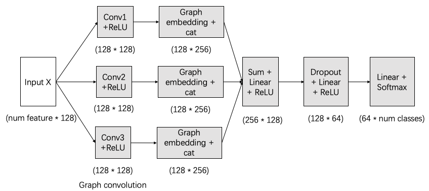
Next, we specify the training of a GNN. We first generate a set of valid graphs manually by running $\mathtt{Verifier}$. We then set a value threshold and label the generated graph a good graph (with value $1$) or a poor graph (with value $0$) based on whether the objective value is above or below the threshold. We then utilize these labeled graphs to train a classifier by GNN designed above to return a value as a softmax value of the probability. The input of the GNN is the node information that the node type, maximum utilization, position and bandwidth utilization in time $t=0,1,2,...,23$, and the adjacent matrix of the graph. For every layer of GNN, the overall activation function is given by

$$H(l+1)=\sigma(D^{-1/2}(\bm{x}+I)D^{1/2}H(l)W(l)).$$ (7)

Here $H(l)$ is the $l$-th layer input and $H(0)=X$ is the input. $\bm{x}$ is the adjacency matrix of graph $G$, $I$ is the identity matrix, $D$ is the degree matrix of graph $G$. $W(l)$ is the parameter in the $l$-th layer. $\sigma(\cdot)$ is the activation function to introduce non-linearity property in this GNN.

IV-B4 DRL framework implementation

In the DRL framework, we use the Advantage Actor-Critic algorithm (A2C) algorithm [12] to learn the RL agent. The RL agent uses the policy $\pi_{\theta}(a|s)$ to search graphs as an actor shown as a probability distribution. The critic $V^{\pi}(s)$ utilizes the reward calculated by the initial objective value from $\mathtt{Verifier}$ algorithm or the label value of GNN for simplification to evaluate the performance of a graph. We utilize multi-layer perceptrons as the basic structure of parameterized policy network and value network. We use the stable baselines3 framework [16] to help finish implementation and train the agent. The key information and hyper-parameters are shown in Table III.

TABLE III: Key information and hyper-parameters in RL training.

Parameters	Value	Parameters	Value
Policy Network	$64$, tanh, $64$, tanh, Linear	Total timesteps	$2\cdot 10^{6}$/$10^{6}$/$10^{5}$
Value Network	$64$, tanh, $64$, tanh, Linear	Discount factor $\gamma$	$0.99$
GAE $\lambda$	$1.0$	Learning rate	$7\cdot 10^{-4}$

In RL training, the algorithm first initializes the parameters of policy. For each epoch, based on the policy, several actions are sampled corresponding to new graphs. By repeatedly choosing from the sampled actions for $H$ steps, the critic finally finds the best graph that gives the highest reward. At the end of the epoch, we compute the policy gradient loss (entropy loss) and critic gradient loss (value loss) and update the parameters. The entropy loss and value loss derived by the gradient loss are regarded as representatives of exploration and exploitation metrics.

IV-C Benchmark Comparison and Experiments

In the experiment, we test the performance of DRL method with two different datasets specified in Section IV-A. In order to show that RL policy helps search a graph with satisfied objective value, we compare A2C-GS with the one-step optimization algorithm shown in Algorithm 8 as a basic method by utilizing prior knowledge of human experts for topology search. Besides, we compare A2C-GS with random policy as another benchmark method. Random policy means that we randomly choose an action in the full action space to generate a graph by randomly building or removing a few links, which enables us to show that RL policy learns the ability to optimize the graph.

IV-C1 Small dataset

In the small dataset, the graph has $8$ nodes ($2T$+$3H$+$3J$) with information explained in Section IV-A. The initial topology has $11$ edges. The maximum distance of the connected edge is $500$m. Thus, $20$ edges can be connected in total. We use A2C-GS to train the agent under the full space with $2^{20}$ choices and compressed space with $10$ combinations using the method in Section IV-B2. Initially, there are $2$ components that all nodes are type-$H$ (one has $2$ nodes and one has $1$ node) and $1$ component that all nodes are type-$J$ with $3$ nodes. The overall choices of step $1\sim 3$ are that, for the component with $2$ nodes, there are $2$ choices and for the component with $3$ nodes, there are $5$ choices. In the fourth step and fifth step, we use one choice that guarantees the management requirements.

Figure 5: Entropy and value loss of RL training. (a) and (d) are for the agent trained in the full space for $10^{6}$ steps. (b) and (e) are for the agent trained in compressed space for $10^{5}$ steps (AC means action compression). (c) and (f) are for the agent trained in compressed space with GNN classifier for $10^{5}$ steps.

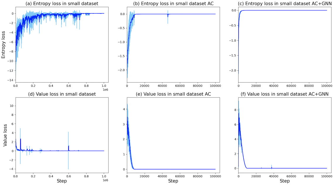
Fig. 5 shows the entropy loss and value loss of training an RL agent in the small dataset, which demonstrates convergence in different training settings. Specifically, training the agent in the original full space requires $10^{6}$ steps for convergence, while it only needs $5\cdot 10^{4}$ steps to guarantee the convergence of training in our defined sub-space.

Figure 6: Left: Frequency of the scores under topologies found by different policies in small dataset. Right: Testing results for different policies in small dataset.

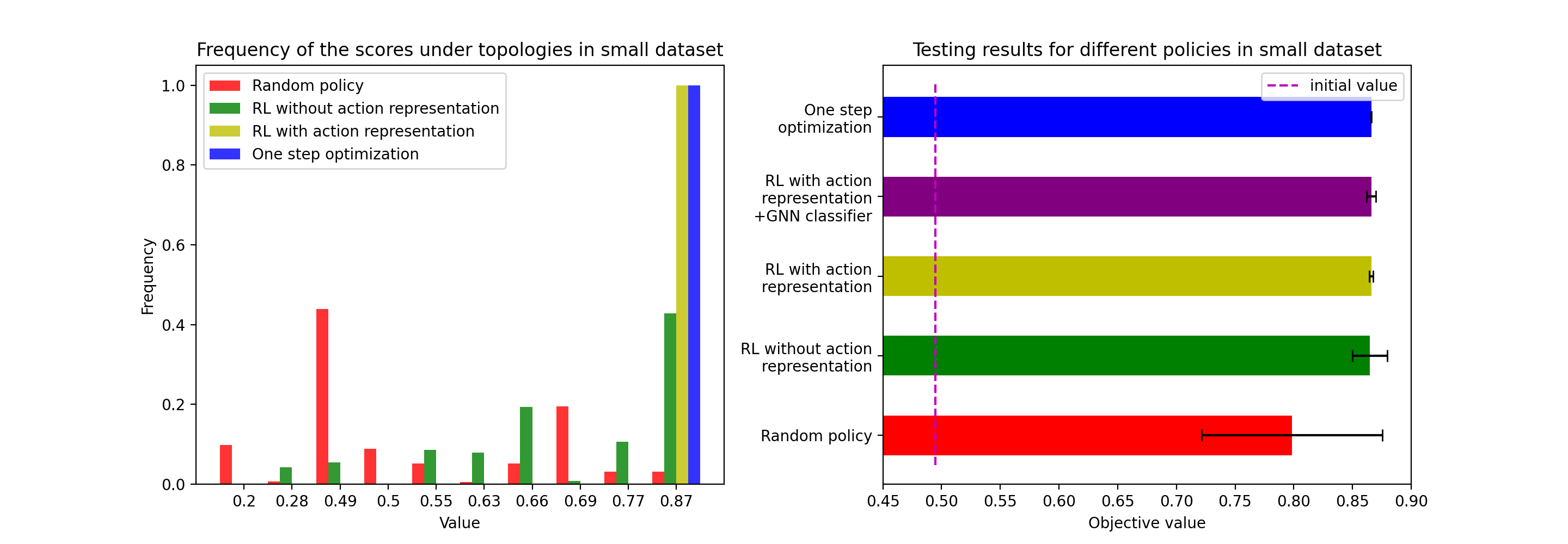
The left figure in Fig. 6 shows the frequency of the scores by different methods The frequencies are computed as follows. First, initialize the environment with a random graph and search one graph by the policy, calculate the score of the graph, repeat the process for $5\cdot 10^{4}$ times and compute the frequency of the scores. The fraction of time the RL agent trained in full space finds the best graph is roughly $40\%$ (green), which is much higher than that of the random policy (red, less than $5\%$). It shows that A2C-GS finds the best graph with a higher success rate than the random policy without any prior knowledge. Moreover, the fraction that the RL agent trained in compressed space finds the best graph is nearly $100\%$ (yellow), which shows that by action compression, the RL agent achieves a better performance. We note that the one-step optimization also finds the optimal graph (blue). This is due to the small scale of the dataset. We will see later that in a larger scale experiment, A2C-GS outperforms one-step optimization significantly.

The right figure in Fig. 6 shows the testing results of different methods, with the mean values shown in colored bars, and the standard deviations shown in black error bar. Specifically, for a given random graph, we use the policy to search five graphs and pick the maximum objective value among them. We repeat the process for $5\cdot 10^{4}$ times, and calculate the mean value and standard deviation among different random seeds. We see that the RL policy (green, $0.8648\pm 0.0148$) performs better than random policy (red). In addition, RL policy trained in compressed space further improves the performance ($0.8660\pm 0.0017$).

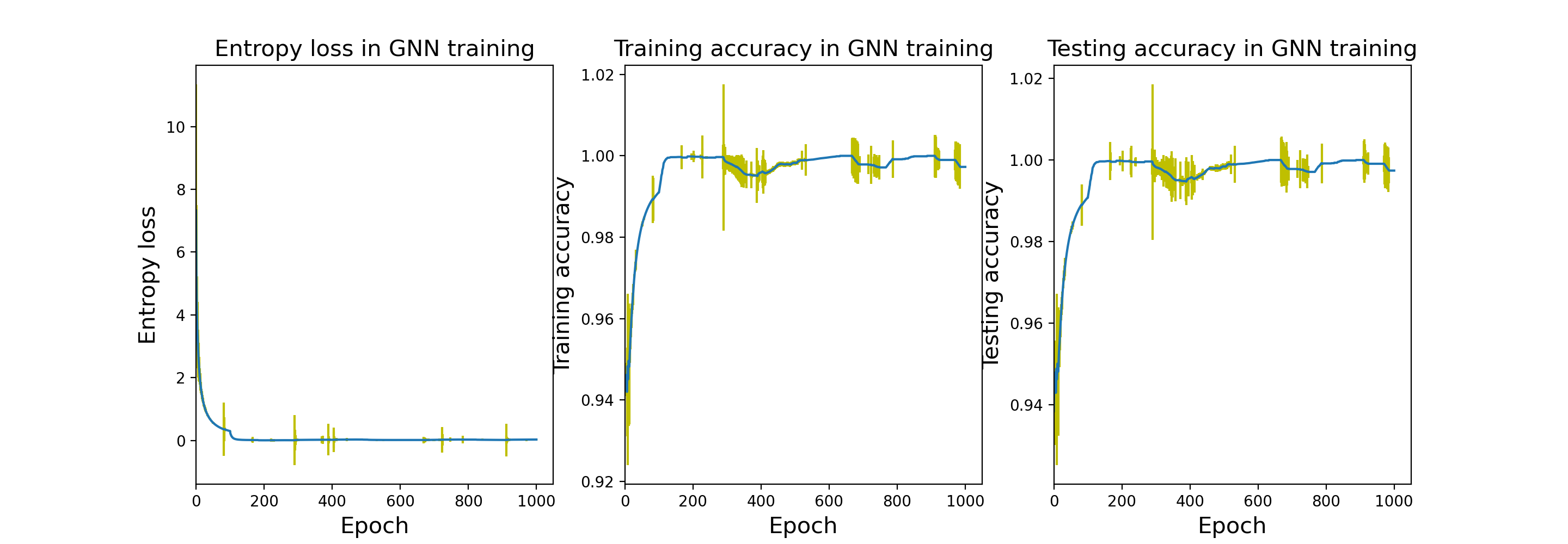
Under the same space setting in RL training, we train a GNN classifier using the structure shown in Fig. 4 and examine the training and testing accuracy of the GNN. We use the Adam optimizer with the learning rate $0.005$ and the threshold value $0.8$ and repeat training $10^{3}$ epochs for $5$ times by initializing the parameter of GNN with different random seeds. Fig. 7 shows the results of the GNN training with the average value and the standard deviation of the entropy loss, training accuracy and testing accuracy. The entropy loss converges to $10^{-4}$, the training accuracy and testing accuracy is higher than $99\%$, which shows that the GNN can classify a graph in high accuracy.

Figure 7: GNN training with entropy loss, training accuracy and testing accuracy in small dataset.

The right figure in Fig. 6 also shows the testing results of the RL agent trained in compressed space adding GNN classifier with similar mean value and higher standard deviation (blue, $0.8660\pm 0.0039$). In the small dataset case, since the topology structure can be verified easily by the $\mathtt{Verifier}$ algorithm, GNN does not show its full advantage in RL training, and algorithms need roughly $10$ hours to train policy with action compression. However, we will see in the large-scale dataset that the introduction of GNN greatly reduces the running time.

IV-C2 Large dataset

In the large dataset, the graph has $23$ nodes ($2T$+$5H$+$16J$) with information explained in Section IV-A. The initial topology has $33$ edges. The maximum distance of the connected edge is $5$km with a total of $72$ edges that can be connected. Therefore, the number of the full action space is $4.7\times 10^{21}$, in which case the agent suffers from the curse of dimensionality, and it is critical for the agent to learn in our compressed action sub-space for higher learning efficiency.

The action sub-space is defined in Section IV-B2. In order to show the trade-off between efficiency and performance, we conduct experiments in two different action sub-spaces, one is smaller with fewer possible actions while another one is larger. We illustrate our design of the two action sub-spaces as below. Initially, there are two components, one with $5$ type-$H$ nodes and another with $16$ type-$J$ nodes. In the large space case, we do not restrict the possible actions for the first basic component. If we choose $m_{i}=1$, we restrict that there is one choice in step $2\sim 5$ that guarantees the management requirements. Instead, if we choose $m_{i}=2$, we restrict the second step in the set $\{(15,1),(14,2)\}$ (here $(15,1)$ means a choice in the second step that one component has $15$ nodes and another has $1$ node as an example). We have no compression on step $3$ and we restrict that there is one choice in step $4\sim 5$ that guarantees the management requirements too. The design of small space has one difference that if we choose $m_{i}=2$ in the first step for the component with $16$ nodes, we restrict that there is one choice $(15,1)$ in the second step. The design helps implementation of training an RL agent and allows us to compare the performance of RL agent trained under different size of action spaces.

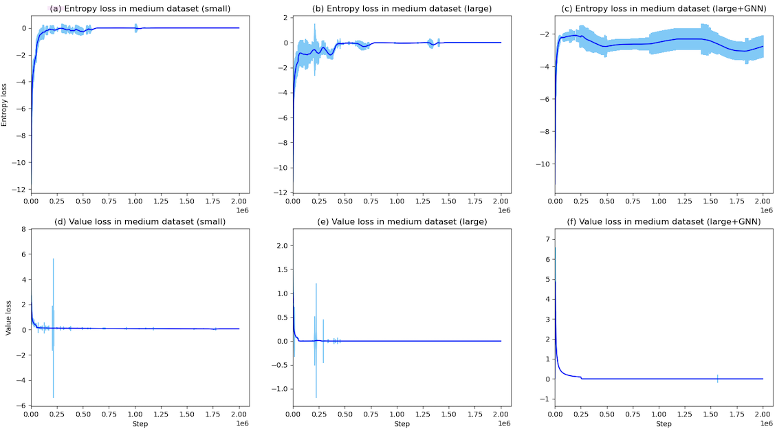
Fig. 8 shows the entropy loss and value loss of training RL agent in a large dataset. Without the GNN classifier, it demonstrates convergence in different training settings. However, the entropy loss cannot converge to nearly $0$ when training an RL agent with GNN classifier. This is because in the GNN training, we use a threshold to cluster the graphs. Thus, there can be multiple graphs with the objective value being larger than the threshold and the final RL policy can sample from multiple idealized graphs, leading to non-zero entropy loss. The value loss still converges to $10^{-7}\sim 10^{-11}$, which confirms the observation.

Figure 8: Entropy and value loss of RL training. (a)(d) is the agent trained in the small space. (b)(e) is the agent trained in large space. (c)(f) is the agent trained in large space with a GNN classifier. All the algorithms run $2\cdot 10^{6}$ steps

The histogram of the scores in the large dataset is shown in the left figure Fig. 9. The horizontal axis shows the regions of the scores. The vertical axis is the frequency that the score of a chosen graph is in the region. The frequencies are computed as follows. Given a random graph, search $30$ graphs by the trained agent, calculate the scores and choose the graph with maximum score. Repeat this process for $5\cdot 10^{4}$ times and compute the frequency.

We notice that the RL policy (yellow and blue bars) performs better than the random policy (red bar). The RL policy trained with a small space generates graphs whose scores are between $0.4\sim 0.6$. The RL policy trained in large space generates graphs with scores larger than $0.6$. This means that the RL agent has the ability to find a good graph. We also compare the results of the RL agent with one-step optimization. In contrast to the small dataset case, where RL and the one-step policy achieve similar performance, here the RL policy performs significantly better than the one-step optimization method. This illustrates that A2C-GS scales much better than human heuristic methods.

Figure 9: Left: Frequency of the scores under typologies found by different policies in large dataset. Right: Testing results for different policies in large dataset.

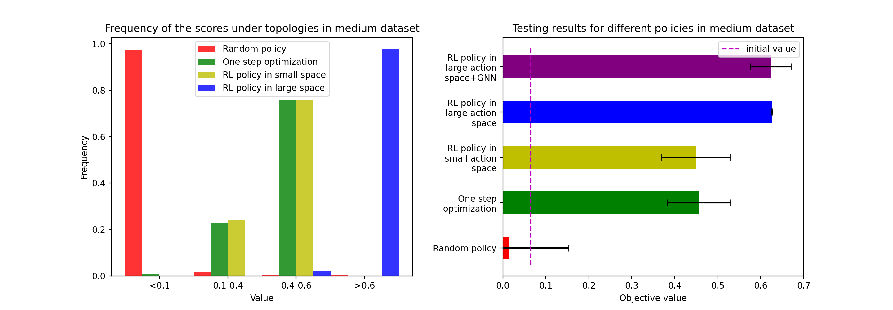
The right figure in Fig. 9 is the testing results of different methods. The values are calculated in the same way as the right figure in Fig. 6. The results show that RL policy trained in compressed space gains better average objective values compared with random policy that fails to find an idealized graph in huge full action space. Compared to one-step optimization, which achieves an average value of $0.4560$, the RL agent trained in small space gains a similar mean value ($0.4499$) while the RL agent trained in large space outperforms the value ($0.6266$). This means that enlarging the searching space helps generate a better policy. The mean value, standard deviation and curve of entropy loss of the RL agent trained in small space and large space also confirm this observation. If the compressed space is chosen appropriately, an RL agent can be trained efficiently and achieve better performance.

Under the same configuration of RL training under large space, we examine the training and testing accuracy of the GNN classifier as in the small dataset. Different from training GNN in small dataset, we use an objective value $0.6$ as the threshold value and train the GNN with $2\cdot 10^{3}$ epochs. The GNN training results are shown in Fig. 10. The entropy loss converges to $10^{-2}$ and the final training accuracy and testing accuracy are higher than $99\%$, which shows that the GNN can classify a graph in high accuracy.

Figure 10: GNN training curve with entropy loss, training and testing accuracy in large dataset.

The right figure in Fig. 9 shows the testing results in RL training using the GNN classifier (blue bar). Compared to the RL agent trained in large space without GNN, the mean value is slightly smaller ($0.6230$) and the standard deviation is larger ($0.0471$). This is expected, as GNN trades off performance for efficiency. The advantage of using GNN is that, in cases where running $\mathtt{Verifier}$ algorithm needs more time, GNN helps improve the efficiency of training RL algorithm, i.e., we need $4$ days to train RL agent with the $\mathtt{Verifier}$ in the large dataset, but we only use $2$ days to train RL agent with the GNN classifier. We note that even with a slight performance loss, the RL agent still performs better than the one-step optimization.

Fig. 11 shows the topology optimization results in the $23$-node case with the relative position. In the initial graph, there are $2$ primary main paths $p_{P}^{(1)}=\{1-7-8-2\}$ and $p_{P}^{(2)}=\{1-9-10-11-2\}$ and $3$ secondary main paths $p_{S}^{(1)},p_{S}^{(2)},p_{S}^{(3)}$ shown in the figure. The bandwidth utilization of $p_{S}^{(1)}$ is large because the maximum utilization of type-$H$ node $9$ and $10$ is low, so $Flow(p_{S}^{(1)},t)$ is much higher than the benchmark bandwidth utilization $B(t)$ described in IV-A1, and the sub ratio is large because there are $4$ nodes in the sub path. At time $t=0,B(0)=0.07$ while $Flow(p_{S}^{(1)},0)=0.12$. When $\epsilon=0.4$, we see that $\mathbb{I}\left(\left|\frac{Flow(p_{S}^{(1)},0)}{B(0)}-1\right|\leq\epsilon\right)=0$ and $Sratio(p_{S}^{(1)})=0.4$, which suffers a loss. This unbalance among paths results in a low objective value ($0.0653$). One-step optimization constructs two paths, a primary main path $p^{\prime}_{P}=\{1-9-\cdots-8-2\}$ and a secondary main path $p^{\prime}_{S}$ shown in the figure. The maximum utilization of node $2$ is larger than that of node $9$, so this path can bear traffic pressure $Flow(p^{\prime}_{S},0)=0.08$, which is close to $B(0)$. Hence, it achieves a $0.4945$ objective value. After training the RL agent, RL policy finds that generating two paths $p^{\prime\prime(1)}_{S},p^{\prime\prime(2)}_{S}$ (shown in the figure) helps because new paths guarantee that both of the bandwidth utilization are close to $B(0)$, i.e., $Flow(p^{\prime\prime(1)}_{S},0)=0.072,Flow(p^{\prime\prime(2)},0)=0.8$. So it achieves a higher objective value $0.6390$.

Figure 11: The initial topology structure and the optimized topology structure by one-step method and A2C-GS. The type-$T$,type-$H$ and type-$J$ nodes are in orange, red, blue colors, respectively. Initially, there exists a heavily-loaded path $p_{S}^{(1)}=\{9-12-13-14-15-10\}$ in red lines attaching nodes $16\sim 19$ as elements in the sub path drawn in green lines. At $t=0,Flow(p_{S}^{(1)},0)=0.12$, which is much larger than the value of paths $p_{S}^{(2)}=\{1-3-4-5-6-2\}$ ($0.04$) and $p_{S}^{(3)}=\{2-23-22-20-11\}$ ($0.03$, and $p_{S}^{(3)}$ includes a hang node $21$). It results in a low objective value ($0.0653$). One-step optimization generates a new path $p^{\prime}_{S}=\{2-6-\cdots-12-9\}$ attaching node $23$ in the sub path with $Flow(p^{\prime}_{S},0)=0.08$. Thus, it achieves a better objective value ($0.4945$). A2C-GS optimizes the topology by generating two new paths $p^{\prime\prime(1)}_{S}=\{10-6-23-11\}$,$p^{\prime\prime(2)}_{S}=\{2-5-\cdots-12-9\}$ with $Flow(p^{\prime\prime(1)}_{S},0)=0.072$, $Flow(p^{\prime\prime(2)}_{S},0)=0.08$ achieving a higher objective value ($0.6390$).

V Conclusion

In this paper, we consider the problem of network topology optimization with management constraints. We propose a deep reinforcement learning framework called A2C-GS, which consists of a verification model to testify the graph, calculate the objective value and generate data, an action compression method to eliminate searching space, and a GNN classifier to replace the $\mathtt{Verifier}$ algorithm to enable efficient topology search. We conduct extensive experiments based on small scale and large scale datasets. The results show that A2C-GS outperform the human-expert based one-step optimization method in finding optimal network topologies.

Appendix A One-step optimization pesudo codes

Here we propose one-step optimization method by constructing new components as the benchmark algorithm to compare with A2C-GS. It is useful in a small dataset while in a large topology network, it would suffer failure. The details of this algorithm are described as follows.

1:  Input: Basic graph $G=(V,E)$, the benchmark $B(t)$, threshold value $D_{\max}$, $\epsilon$.

2:  for $Type=H,J$ do

3:     Generate $G^{\prime}=(V^{\prime},E^{\prime})$ that $\forall v\in V,\text{if }Type(v)=Type,v\in V^{\prime}$; $\forall e\in E^{\prime},Dist(e)\leq D_{\max}$. Run $\mathtt{BFS}$ algorithm in $G^{\prime}$ to generate buffer $\mathcal{D}_{Type}=\{D_{i}=\{v_{i_{1}},...,v_{i_{n}}\}\}_{i=1}^{d}$.

4:     while $\exists D_{i},|D_{i}|>0$ do

5:        For every group $D_{i}$, sort nodes based on $\sum_{t}Flow(v_{i},t)$ in decrease order as $v_{i_{1}}^{\prime},...,v_{i_{n}}^{\prime}$. For every node group $v_{i_{1}}^{\prime},...,v_{i_{u}}^{\prime}$, where $u=1,...,n$, calculate:

$$Utility(u)=\frac{1}{24}\sum_{t=1}^{24}\mathbb{I}\left(\left|\frac{\sum_{v_{k}=v_{i_{1}}^{\prime},...,v_{i_{u}}^{\prime}}Flow(v_{k},t)}{\max_{v\in V}U_{\max}(v)}-B(t)\right|/B(t)\leq\epsilon\right)$$

6:        Set that $U=\text{argmax}_{u}Utility(u),u_{0}=\max_{u}(U)$, $D_{i}\leftarrow D_{i}\backslash\{v_{i_{1}}^{\prime},...,v_{i_{u_{0}}}^{\prime}\}$. For group $D^{\prime\prime}=\{v_{i_{1}}^{\prime},...,v_{i_{u_{0}}}^{\prime}\}$, run $\mathtt{BFS}$ algorithm in $G^{\prime\prime}=(D^{\prime\prime},E^{\prime\prime}),(\forall e\in E^{\prime\prime},Dist(e)\leq D_{\max})$ to search the connected component $\tilde{D}_{1},...,\tilde{D}_{\tilde{d}}$ and add these into the buffer $\mathcal{D}_{Type}$.

7:     end while

8:  end for

9:  Set edge buffer $\mathcal{E}$. $\forall D_{h}\in\mathcal{D}_{H},D_{j}\in\mathcal{D}_{J}$, generate $G_{h}=(D_{h},E_{h}),G_{j}=(D_{j},E_{j})$ for connectivity. If $\exists v_{h_{1}},v_{h_{2}}\in D_{h},v_{j_{1}},v_{j_{2}}\in D_{j}$ that $Dist(e_{i})\leq D_{\max},e_{i}=(v_{j_{i}},v_{h_{i}}),i=1,2$, add $e_{i}$ into $\mathcal{E}$. Generate $\tilde{G}=(V,\tilde{E})$ that $\tilde{E}=(\cup_{h}E_{h})\cup(\cup_{j}E_{j})\cup\mathcal{E},\forall E_{h},E_{j}$.

10:  Return $\tilde{G}$.

Algorithm 8 One step optimization method

References

- [1] Oleg Bondarenko, Dmytro Ageyev, and Othman Mohammed. Optimization model for 5g network planning. In 2019 IEEE 15th International Conference on the Experience of Designing and Application of CAD Systems (CADSM), pages 1–4. IEEE, 2019.
- [2] Quentin Cappart, Thierry Moisan, Louis-Martin Rousseau, Isabeau Prémont-Schwarz, and Andre Cire. Combining reinforcement learning and constraint programming for combinatorial optimization. arXiv preprint arXiv:2006.01610, 2020.
- [3] Wenqi Fan, Yao Ma, Qing Li, Yuan He, Eric Zhao, Jiliang Tang, and Dawei Yin. Graph neural networks for social recommendation. In The world wide web conference, pages 417–426, 2019.
- [4] Matthias Fey and Jan Eric Lenssen. Fast graph representation learning with pytorch geometric. arXiv preprint arXiv:1903.02428, 2019.
- [5] Ori Gerstel, Clarence Filsfils, Thomas Telkamp, Matthias Gunkel, Martin Horneffer, Victor Lopez, and Arturo Mayoral. Multi-layer capacity planning for ip-optical networks. IEEE Communications Magazine, 52(1):44–51, 2014.
- [6] Beneyam Berehanu Haile, Edward Mutafungwa, and Jyri Hämäläinen. A data-driven multiobjective optimization framework for hyperdense 5g network planning. IEEE Access, 8:169423–169443, 2020.
- [7] A Hanif Halim and I Ismail. Combinatorial optimization: comparison of heuristic algorithms in travelling salesman problem. Archives of Computational Methods in Engineering, 26(2):367–380, 2019.
- [8] Shiwen He, Shaowen Xiong, Yeyu Ou, Jian Zhang, Jiaheng Wang, Yongming Huang, and Yaoxue Zhang. An overview on the application of graph neural networks in wireless networks. IEEE Open Journal of the Communications Society, 2021.
- [9] Liang Huang, Suzhi Bi, and Ying-Jun Angela Zhang. Deep reinforcement learning for online computation offloading in wireless powered mobile-edge computing networks. IEEE Transactions on Mobile Computing, 19(11):2581–2593, 2019.
- [10] Chaitanya K Joshi, Quentin Cappart, Louis-Martin Rousseau, and Thomas Laurent. Learning tsp requires rethinking generalization. arXiv preprint arXiv:2006.07054, 2020.
- [11] Gongqi Lin, Sieteng Soh, Mihai Lazarescu, and Kwan-Wu Chin. Power-aware routing in networks with delay and link utilization constraints. In 37th Annual IEEE Conference on Local Computer Networks, pages 272–275. Ieee, 2012.
- [12] Volodymyr Mnih, Adria Puigdomenech Badia, Mehdi Mirza, Alex Graves, Timothy Lillicrap, Tim Harley, David Silver, and Koray Kavukcuoglu. Asynchronous methods for deep reinforcement learning. In International conference on machine learning, pages 1928–1937. PMLR, 2016.
- [13] China Mobile. Ai tour of 2020 china mobile maker marathon, complex network modeling competition: Network topology optimization. https://js.aiiaorg.cn/match/matchitem/84. 2020.
- [14] Mohammadreza Nazari, Afshin Oroojlooy, Lawrence Snyder, and Martin Takác. Reinforcement learning for solving the vehicle routing problem. Advances in neural information processing systems, 31, 2018.
- [15] Ling Pan, Qingpeng Cai, Zhixuan Fang, Pingzhong Tang, and Longbo Huang. A deep reinforcement learning framework for rebalancing dockless bike sharing systems. In Proceedings of the AAAI conference on artificial intelligence, volume 33, pages 1393–1400, 2019.
- [16] Antonin Raffin, Ashley Hill, Adam Gleave, Anssi Kanervisto, Maximilian Ernestus, and Noah Dormann. Stable-baselines3: Reliable reinforcement learning implementations. Journal of Machine Learning Research, 2021.
- [17] Abdellah Rezoug, Mohamed Bader-El-Den, and Dalila Boughaci. Guided genetic algorithm for the multidimensional knapsack problem. Memetic Computing, 10(1):29–42, 2018.
- [18] Dorabella Santos, Amaro De Sousa, Filipe Alvelos, Mateusz Dzida, and Michał Pióro. Optimization of link load balancing in multiple spanning tree routing networks. Telecommunication Systems, 48(1):109–124, 2011.
- [19] Yunhao Tang, Shipra Agrawal, and Yuri Faenza. Reinforcement learning for integer programming: Learning to cut. In International Conference on Machine Learning, pages 9367–9376. PMLR, 2020.
- [20] David P Williamson and David B Shmoys. The design of approximation algorithms. Cambridge university press, 2011.
- [21] Peng Yi, Yiguang Hong, and Feng Liu. Initialization-free distributed algorithms for optimal resource allocation with feasibility constraints and application to economic dispatch of power systems. Automatica, 74:259–269, 2016.
- [22] Jiaxuan You, Bowen Liu, Zhitao Ying, Vijay Pande, and Jure Leskovec. Graph convolutional policy network for goal-directed molecular graph generation. Advances in neural information processing systems, 31, 2018.
- [23] Hang Zhu, Varun Gupta, Satyajeet Singh Ahuja, Yuandong Tian, Ying Zhang, and Xin Jin. Network planning with deep reinforcement learning. In Proceedings of the 2021 ACM SIGCOMM 2021 Conference, pages 258–271, 2021.