Zeta-function and $\mu^{*}$-Zariski pairs of surfaces

Abstract.

A Zariski pair of surfaces is a pair of complex polynomial functions in $\mathbb{C}^{3}$ which is obtained from a classical Zariski pair of projective curves $f_{0}(z_{1},z_{2},z_{3})=0$ and $f_{1}(z_{1},z_{2},z_{3})=0$ of degree $d$ in $\mathbb{P}^{2}$ by adding a same term of the form $z_{i}^{d+m}$ ($m\geq 1$) to both $f_{0}$ and $f_{1}$ so that the corresponding affine surfaces of $\mathbb{C}^{3}$ — defined by $g_{0}:=f_{0}+z_{i}^{d+m}$ and $g_{1}:=f_{1}+z_{i}^{d+m}$ — have an isolated singularity at the origin and the same zeta-function for the monodromy associated with their Milnor fibrations (so, in particular, $g_{0}$ and $g_{1}$ have the same Milnor number). In the present paper, we show that if $f_{0}$ and $f_{1}$ are “convenient” with respect to the coordinates $(z_{1},z_{2},z_{3})$ and if the singularities of the curves $f_{0}=0$ and $f_{1}=0$ are Newton non-degenerate in some suitable local coordinates, then $(g_{0},g_{1})$ is a $\mu^{*}$-Zariski pair of surfaces, that is, a Zariski pair of surfaces whose polynomials $g_{0}$ and $g_{1}$ have the same Teissier’s $\mu^{*}$-sequence but lie in different path-connected components of the $\mu^{*}$-constant stratum. To this end, we prove a new general formula that gives, under appropriate conditions, the Milnor number of functions of the above type, and we show (in a general setting) that two polynomials functions lying in the same path-connected component of the $\mu^{*}$-constant stratum can always be joined by a “piecewise complex-analytic path”.

1. Introduction

Consider two reduced homogeneous polynomial functions $f_{0}(z_{1},z_{2},z_{3})$ and $f_{1}(z_{1},z_{2},z_{3})$ of degree $d$ in $\mathbb{C}^{3}$ which are “convenient” (i.e., the Newton boundaries of $f_{0}$ and $f_{1}$ intersect each coordinate axis) and such that the corresponding curves $C_{0}$ and $C_{1}$ in the complex projective plane $\mathbb{P}^{2}$ makes a “Zariski pair”. This means that there are regular neighbourhoods $N(C_{0})$ and $N(C_{1})$ of $C_{0}$ and $C_{1}$, respectively, such that the pairs $(N(C_{0}),C_{0})$ and $(N(C_{1}),C_{1})$ are homeomorphic while the pairs $(\mathbb{P}^{2},C_{0})$ and $(\mathbb{P}^{2},C_{1})$ are not (see [21, 3, 4]). We suppose that the singularities of the curves are located in $z_{1}z_{2}z_{3}\not=0$. Now, add a same term of the form $z_{i}^{d+m}$ (where $m$ is an integer $\geq 1$) to both $f_{0}$ and $f_{1}$ so that the corresponding affine surfaces of $\mathbb{C}^{3}$, defined by $g_{0}:=f_{0}+z_{i}^{d+m}$ and $g_{1}:=f_{1}+z_{i}^{d+m}$ respectively, have an isolated singularity at the origin. As in [14, 15], we say that the pair $(g_{0},g_{1})$ is a Zariski pair of surfaces (or a Zariski pair of links) if $g_{0}$ and $g_{1}$ have the same zeta-function for the monodromy associated with their Milnor fibrations (so, in particular, $g_{0}$ and $g_{1}$ have the same Milnor number). The main, but not unique, goal of the present paper is to show that if the singularities of the curves $C_{0}$ and $C_{1}$ are Newton non-degenerate in some suitable local coordinates, then $(g_{0},g_{1})$ is a Zariski pair of surfaces for which $g_{0}$ and $g_{1}$ have the same Teissier’s $\mu^{*}$-sequence while lying in different path-connected components of the corresponding $\mu^{*}$-constant stratum (see Theorem 5.1). As in [15], we call such a special Zariski pair of surfaces a $\mu^{*}$-Zariski pair of surfaces.

The main tool we use in the proof is a formula, established by the second named author in [14], which gives the zeta-function of the monodromy associated with the Milnor fibration of an “almost Newton non-degenerate function”. (The class of almost Newton non-degenerate functions, less rigid than the class of Newton non-degenerate functions, enjoys many interesting properties as shown in [14, 15]. The components $g_{0}$ and $g_{1}$ of our $\mu^{*}$-Zariski pair of surfaces are such functions.) We shall apply this formula for the zeta-function in order to show a crucial step of the proof of Theorem 5.1. This step is another general formula (hereafter referred to as “shift formula”, see Theorem 3.2) that gives the Milnor number of a function in $\mathbb{C}^{n}$ of the form $g=f+z_{i}^{d_{i}+m}$ ($m\geq 1$). Here, $f$ is a weighted homogeneous polynomial (for some weight $\mathbf{w}=(w_{1},\ldots,w_{n})$) of the form

$$f=a_{1}z_{1}^{d_{1}}+\cdots+a_{n}z_{n}^{d_{n}}+\sum_{\alpha=(\alpha_{1},\ldots,\alpha_{n})}a_{\alpha}z_{1}^{\alpha_{1}}\cdots z_{n}^{\alpha_{n}}$$

such that the singular locus of $V:=f^{-1}(0)$ is $1$-dimensional and for any proper subset $I\subsetneq\{1,\ldots,n\}$ the restriction of $f$ to $\mathbb{C}^{I}:=\{(z_{1},\ldots,z_{n})\in\mathbb{C}^{n}\mid z_{i}=0\mbox{ and }i\notin I\}$ is Newton non-degenerate. We also assume that $f$ satisfies the following “Newton pre-non-degeneracy condition”. Take a toric modification $\hat{\pi}\colon X\to\mathbb{C}^{n}$ compatible with the dual Newton diagram of $f$, and consider the divisor $\hat{E}(\mathbf{w})$ associated with the weight $\mathbf{w}$. We say that $f$ is Newton pre-non-degenerate if each singularity $\mathbf{p}\in E(\mathbf{w}):=\hat{E}(\mathbf{w})\cap\widetilde{V}$ (where $\widetilde{V}$ denotes the strict transform of $V$) is convenient and Newton non-degenerate in suitable local coordinates (i.e., for appropriate local coordinates near $\mathbf{p}$, the hypersurface $E(\mathbf{w})$ of $\hat{E}(\mathbf{w})$ is defined by a convenient Newton non-degenerate function). For more details, see Definition 3.1. Under these assumptions on $f$, we show that the function $g=f+z_{i}^{d_{i}+m}$ is almost Newton non-degenerate, so that, in order to obtain its Milnor number, it is enough to compute the degree of its zeta-function — a zeta-function which can be effectively computed using [14].

Another ingredient that plays an important role in the proof of Theorem 5.1 is the following property of $\mu^{*}$-constant strata. Suppose $f$ and $f^{\prime}$ are polynomial functions on $\mathbb{C}^{n}$ that vanish at the origin. If $f$ and $f^{\prime}$ (as germs of analytic functions at the origin) lie in the same path-connected component of the $\mu^{*}$-constant stratum, then $f$ and $f^{\prime}$ can always be joined by a “piecewise complex-analytic path” (see Definition 4.7 and the comment after it for the precise meaning). Up to our knowledge, this property has never been observed so far. We shall prove it in Section 4 (see Theorem 4.9). Certainly, this latter result as well as a similar one concerning the $\mu$-constant stratum (which we also prove in Section 4) may be useful in many situations in singularity theory.

Contents

1. 1 Introduction
2. 2 Formula for the zeta-function of an almost Newton non-degenerate function
   1. 2.1 The A’Campo formula
   2. 2.2 Dual Newton diagram
   3. 2.3 Toric modification
   4. 2.4 The Varchenko formula
   5. 2.5 Almost Newton non-degenerate functions
   6. 2.6 The Oka formula
3. 3 A shift formula for the Milnor number
4. 4 On the structure of the $\mu$-constant and $\mu^{*}$-constant strata
   1. 4.1 The semi-algebraic set $W(n,m,\mu)$
   2. 4.2 The semi-algebraic set $W^{*}(n,m,\mu^{*}_{n})$
   3. 4.3 Path-connected components and piecewise complex-analytic paths
5. 5 Construction of $\mu^{*}$-Zariski pairs of surfaces
   1. 5.1 Zeta-multiplicity and zeta-multiplicity factor
   2. 5.2 Examples of $\mu^{*}$-Zariski pairs of surfaces

2. Formula for the zeta-function of an almost Newton non-degenerate function

In this section we recall a formula, established by the second named author in [14], which gives the zeta-function of the monodromy associated with the Milnor fibration at the origin of an almost Newton non-degenerate function. This formula generalizes the classical Varchenko formula, given in [20], which is about Newton non-degenerate functions. It will play a crucial role to establish the shift formula for the Milnor number mentioned in the introduction and to construct our $\mu^{*}$-Zariski pair.

Throughout this section, let $\mathbf{z}=(z_{1},\ldots,z_{n})$ be coordinates for $\mathbb{C}^{n}$ ($n\geq 2$), and let $f(\mathbf{z})=\sum_{\alpha}a_{\alpha}\mathbf{z}^{\alpha}$ be a non-constant analytic function defined in a neighbourhood $U$ of the origin $\mathbf{0}\in\mathbb{C}^{n}$. Here, $\alpha=(\alpha_{1},\ldots,\alpha_{n})\in\mathbb{N}^{n}$ and $\mathbf{z}^{\alpha}=z_{1}^{\alpha_{1}}\cdots z_{n}^{\alpha_{n}}$. We assume that $f(\mathbf{0})=0$ and we write $V:=f^{-1}(0)$ for the hypersurface in $U\subseteq\mathbb{C}^{n}$ defined by $f$.

2.1. The A’Campo formula

The starting point for the results of [20, 14] mentioned above is another famous formula for the zeta-function of the monodromy due to A’Campo [1]. In this subsection, we recall this formula in a slightly more general form as given by the second named author in [13].

Let $F$ denote the Milnor fibre of the Milnor fibration of $f$ at $\mathbf{0}$ and let $h\colon F\to F$ be the associated monodromy map. The zeta-function $\zeta_{f,\mathbf{0}}(t)$ of the monodromy associated with the Milnor fibration of $f$ at $\mathbf{0}$ is defined by

$$\zeta_{f,\mathbf{0}}(t):=\prod_{i=0}^{n-1}P_{i}(t)^{(-1)^{i+1}}.$$

Here, $P_{i}(t):=\det(\mbox{Id}-t\cdot h_{*i})$, where $h_{*i}\colon H_{i}(F;\mathbb{Q})\to H_{i}(F;\mathbb{Q})$ is the homomorphism induced by $h$ on the $i$th homology group of $F$ with coefficients in $\mathbb{Q}$. Note that in the special case of isolated singularities, the fibre $F$ is $(n-2)$-connected, so that

$$\zeta_{f,\mathbf{0}}(t):=(1-t)^{-1}P_{n-1}(t)^{(-1)^{n}}$$

and the Milnor number $\mu_{\mathbf{0}}(f)$ of $f$ at $\mathbf{0}$ satisfies the relation

(2.1) $$-1+(-1)^{n}\mu_{\mathbf{0}}(f)=\deg\zeta_{f,\mathbf{0}}(t).$$

(Here, by definition, the degree of a rational function $R(t)=p(t)/q(t)$ is the number $\deg R(t):=\deg p(t)-\deg q(t)$.)

Now, assume we are given a good resolution of the function $f$, that is, a proper holomorphic map $\hat{\pi}\colon X\to U$ from a (complex) analytic manifold $X$ of dimension $n$ to the neighbourhood $U$ satisfying the following two conditions:

1. the restriction $\hat{\pi}\colon X\setminus\hat{\pi}^{-1}(V)\to U\setminus V$ is biholomorphic;

2. if $\hat{\pi}^{-1}(V)=E_{1}\cup\cdots\cup E_{r}\cup E_{r+1}\cup\cdots\cup E_{r+m}$ and $\widetilde{V}=E_{r+1}\cup\cdots\cup E_{r+m}$ denote the irreducible decompositions of the total transform $\hat{\pi}^{-1}(V)$ and of the strict transform $\widetilde{V}$ of $V$ by $\hat{\pi}$, respectively, then the $E_{i}$’s ($1\leq i\leq r+m$) are non-singular and $\hat{\pi}^{-1}(V)$ has only normal crossing singularities.

The second condition means that for any $\mathbf{p}\in\hat{\pi}^{-1}(V)$, if $I$ is the set of indexes $i$ ($1\leq i\leq r+m$) for which $\mathbf{p}\in E_{i}$, then $|I|\leq n$ and there is an analytic coordinate chart $(U_{\mathbf{p}},\mathbf{x}:=(x_{1},\ldots,x_{n}))$ of $X$ at $\mathbf{p}$ together with an injective map $\nu\colon I\to\{1,\ldots,n\}$ such that, in this chart, $E_{i}$ is given by $x_{\nu(i)}=0$ for all $i\in I$.

Now, for all $1\leq i\leq r$, let $m_{i}$ denote the multiplicity along $E_{i}$ of the pull-back function $\hat{\pi}^{*}f$ of $f$ by $\hat{\pi}$, and let

$$E^{\prime}_{i}:=\hat{\pi}^{-1}(0)\cap\Bigg{(}E_{i}\Bigg{\backslash}\widetilde{V}\cup\bigcup_{\begin{subarray}{c}1\leq j\leq r\\ j\not=i\end{subarray}}E_{j}\Bigg{)}.$$

Then the A’Campo–Oka formula for the zeta-function $\zeta_{f,\mathbf{0}}(t)$ says that

(2.2) $$\zeta_{f,\mathbf{0}}(t)=\prod_{i=1}^{r}(1-t^{m_{i}})^{-\chi(E^{\prime}_{i})}$$

where $\chi(E^{\prime}_{i})$ is the Euler–Poincaré characteristic of $E^{\prime}_{i}$ (see [1, Théorème 3] and [13, Chapter I, Theorem (5.2)]). Let us highlight that this formula holds for possibly non-isolated singularities.

Remark 2.1 (see[15, Proposition 11]).

If $\mbox{mult}_{\mathbf{0}}(f)$ is the multiplicity of $f$ at $\mathbf{0}$, then for each $1\leq i\leq r$ we have $m_{i}\geq\mbox{mult}_{\mathbf{0}}(f)$.

To state the formulas by Varchenko and Oka about Newton non-degenerate and almost Newton non-degenerate functions, we first need to recall the notions of dual Newton diagram and toric modification. This is done in §§2.2 and 2.3 below. The formulas by Varchenko and Oka are given in §2.4 and in §2.6 respectively.

2.2. Dual Newton diagram

Here, we recall the notion of dual Newton diagram. For details, we refer the reader to [13, Chapter II, §1 and Chapter III, §3].

Let $M$ be the lattice of Laurent monomials in the variables $z_{1},\ldots,z_{n}$, and let $W$ be the (dual) lattice of (integral) weights on these variables, that is, the lattice of weight functions $\mathbf{w}\colon\{z_{1},\ldots,z_{n}\}\to\mathbb{Z}$. Let

$$M_{\mathbb{R}}:=M\otimes_{\mathbb{Z}}\mathbb{R}\quad\mbox{and}\quad W_{\mathbb{R}}:=W\otimes_{\mathbb{Z}}\mathbb{R}$$

be the corresponding real vector spaces of dimension $n$. Hereafter, we identify these spaces with $\mathbb{R}^{n}$, and to avoid any confusion, we denote the vectors in $M_{\mathbb{R}}$ (respectively, in $W_{\mathbb{R}}$) by row vectors (respectively, by column vectors). So, in particular, a monomial $\mathbf{z}^{\alpha}=z_{1}^{\alpha_{1}}\cdots z_{n}^{\alpha_{n}}\in M$ is identified with the integral row vector $\alpha=(\alpha_{1},\ldots,\alpha_{n})$ while a weight $\mathbf{w}\in W$ is identified with the integral column vector ${}^{t}(w_{1},\ldots,w_{n}):={}^{t}(\mathbf{w}(z_{1}),\ldots,\mathbf{w}(z_{n}))$. Define $M^{+}$ (respectively, $W^{+}$) as the set of all “non-negative” row vectors $(\alpha_{1},\ldots,\alpha_{n})\in M$ (respectively, all “non-negative” column vectors ${}^{t}(w_{1},\ldots,w_{n})\in W$) — that is, $\alpha_{i}\geq 0$ and $w_{i}\geq 0$ for all $1\leq i\leq n$. Define $M_{\mathbb{R}}^{+}$ and $W_{\mathbb{R}}^{+}$ similarly. Again, hereafter we identify $M_{\mathbb{R}}^{+}$ and $W_{\mathbb{R}}^{+}$ with

$$\mathbb{R}^{n}_{\geq 0}:=\{\mathbf{x}=(x_{1},\ldots,x_{n})\in\mathbb{R}^{n}\mid x_{i}\geq 0\mbox{ for all }1\leq i\leq n\}.$$

The elements of $W_{\mathbb{R}}^{+}$ are called weight vectors, and an integral weight vector ${}^{t}(w_{1},\ldots,w_{n})\in W^{+}\setminus\{\mathbf{0}\}$ is called primitive if $\gcd(w_{1},\ldots,w_{n})=1$.

Clearly, the Newton polyhedron $\Gamma_{\!+}(f)$ and the Newton boundary $\Gamma(f)$ of $f$ at $\mathbf{0}$ with respect to the coordinates $\mathbf{z}=(z_{1},\ldots,z_{n})$ can be viewed as subspaces of $M_{\mathbb{R}}^{+}$. We recall that $\Gamma_{\!+}(f)$ (or $\Gamma_{\!+}(f;\mathbf{z})$ when we need to emphasize the coordinates) is defined as the convex hull in $\mathbb{R}^{n}_{\geq 0}$ of the set

$$\bigcup_{\alpha,\,a_{\alpha}\not=0}(\alpha+\mathbb{R}^{n}_{\geq 0})$$

while $\Gamma(f)$ is the union of the compact faces of $\Gamma_{\!+}(f)$.

Let us also recall that a convex polyhedral cone $\sigma\subseteq W_{\mathbb{R}}^{+}$ is a set of the form

(2.3) $$\sigma=C(\mathbf{w}_{1},\ldots,\mathbf{w}_{k}):=\bigg{\{}\sum_{i=1}^{k}\lambda_{i}\mathbf{w}_{i}\in W_{\mathbb{R}}^{+}\mid\lambda_{i}\in\mathbb{R}_{\geq 0}\mbox{ for all }1\leq i\leq k\bigg{\}}.$$

The vectors $\mathbf{w}_{i}\in W_{\mathbb{R}}^{+}$ that appear in (2.3) are called generators of $\sigma$. If they can be taken in $W^{+}$, then $\sigma$ is said to be rational. Any rational convex polyhedral cone $\sigma\subseteq W_{\mathbb{R}}^{+}$ can be uniquely written as $\sigma=C(\mathbf{w}_{1},\ldots,\mathbf{w}_{k})$, where the $\mathbf{w}_{i}$’s are primitive and $k$ is minimal among all possible such expressions (i.e., $\mathbf{w}_{i}\notin C(\mathbf{w}_{1},\ldots,\mathbf{w}_{i-1},\mathbf{w}_{i+1},\ldots,\mathbf{w}_{k})$ for each $1\leq i\leq k$). Hereafter we always assume that cones are generated by the minimal generators. The dimension of a convex polyhedral cone $\sigma\subseteq W_{\mathbb{R}}^{+}$ is its Euclidean dimension. A rational convex polyhedral cone $\sigma=C(\mathbf{w}_{1},\ldots,\mathbf{w}_{k})$ is said to be simplicial if $\mathbf{w}_{1},\ldots,\mathbf{w}_{k}$ are linearly independent over $\mathbb{R}$; it is said to be regular if $\mathbf{w}_{1},\ldots,\mathbf{w}_{k}$ are primitive and can be completed in a basis of the lattice $\mathbb{Z}^{n}$.

A family $\Sigma^{*}$ of rational convex polyhedral cones of $W_{\mathbb{R}}^{+}$ is called a rational convex polyhedral cone subdivision of $W_{\mathbb{R}}^{+}$ if $\Sigma^{*}$ is a finite complex such that

$$W_{\mathbb{R}}^{+}=\bigcup_{\sigma\in\Sigma^{*}}\sigma.$$

Note that since we are dealing with cones having the origin as vertex, we can identify any rational convex polyhedral cone subdivision with its projection on the “hyperplane” of $W_{\mathbb{R}}^{+}\equiv\mathbb{R}^{n}_{\geq 0}$ defined by the equation $x_{1}+\cdots+x_{n}=1$. A rational convex polyhedral cone subdivision $\Sigma^{*}$ of $W_{\mathbb{R}}^{+}$ is called a simplicial cone subdivision of $W_{\mathbb{R}}^{+}$ if every cone $\sigma\in\Sigma^{*}$ is simplicial. A simplicial cone subdivision $\Sigma^{*}$ of $W_{\mathbb{R}}^{+}$ is called a regular simplicial cone subdivision of $W_{\mathbb{R}}^{+}$ if every simplicial cone $\sigma\in\Sigma^{*}$ is regular. Finally, a vertex of a regular simplicial cone subdivision $\Sigma^{*}$ is a primitive weight vector which generates a $1$-dimensional cone of $\Sigma^{*}$.

Now, for any weight vector $\mathbf{w}={}^{t}(w_{1},\ldots,w_{n})\in W_{\mathbb{R}}^{+}$, write $d(\mathbf{w};f)$ for the minimal value of the restriction to $\Gamma_{\!+}(f)$ of the canonical linear map $\ell_{\mathbf{w}}$ defined by

(2.4) $$\ell_{\mathbf{w}}(\alpha):=\sum_{i=1}^{n}\alpha_{i}w_{i},$$

and put

$$\Delta(\mathbf{w};f):=\{\alpha\in\Gamma_{\!+}(f)\mid\ell_{\mathbf{w}}(\alpha)=d(\mathbf{w};f)\}.$$

Clearly, $\Delta(\mathbf{w};f)$ is a face of $\Gamma_{\!+}(f)$. It is a compact face (i.e., it is contained in the Newton boundary $\Gamma(f)$) if and only if $\mathbf{w}$ is a “positive” weight vector (i.e., if $w_{i}>0$ for each $i$).

In order to define the dual Newton diagram, we consider on $W_{\mathbb{R}}^{+}$ the equivalence relation $\sim$ defined for any $\mathbf{w},\mathbf{w}^{\prime}\in W_{\mathbb{R}}^{+}$ as follows:

$$\mathbf{w}\sim\mathbf{w}^{\prime}\Leftrightarrow\Delta(\mathbf{w};f)=\Delta(\mathbf{w}^{\prime};f).$$

For any face $\Delta\subseteq\Gamma_{\!+}(f)$, there is an equivalence class $\Delta^{*}$ which is defined by

$$\Delta^{*}:=\{\mathbf{w}\in W^{+}_{\mathbb{R}}\mid\Delta(\mathbf{w};f)=\Delta\}.$$

For each $(n-1)$-dimensional face $\Delta_{0}\subseteq\Gamma_{\!+}(f)$, there is a unique primitive weight vector $\mathbf{w}(\Delta_{0})\in W^{+}\setminus\{\mathbf{0}\}$ such that $\Delta_{0}=\Delta(\mathbf{w}(\Delta_{0});f)$, and for any face $\Delta\subseteq\Gamma_{\!+}(f)$, the corresponding equivalence class $\Delta^{*}$ is of the form

$$\Delta^{*}=\bigg{\{}\sum_{i=1}^{k}\lambda_{i}\mathbf{w}(\Delta_{i})\in W_{\mathbb{R}}^{+}\mid\lambda_{i}\in\mathbb{R}_{>0}\mbox{ for all }1\leq i\leq k\bigg{\}},$$

where the $\Delta_{i}$’s are the $(n-1)$-dimensional faces of $\Gamma_{\!+}(f)$ containing $\Delta$. The family

$$\{\Delta^{*}\}_{\Delta\subsetneq\Gamma_{\!+}(f)}$$

(where $\Delta$ runs over all proper faces of $\Gamma_{\!+}(f)$) is a partition of $W_{\mathbb{R}}^{+}\setminus\{\mathbf{0}\}\equiv\mathbb{R}^{n}_{\geq 0}\setminus\{\mathbf{0}\}$.

Definition 2.2.

The dual Newton diagram $\Gamma^{*}(f)$ (or $\Gamma^{*}(f;\mathbf{z})$) of $f$ at $\mathbf{0}$ with respect to the coordinates $\mathbf{z}=(z_{1},\ldots,z_{n})$ is the rational convex polyhedral cone subdivision of $W_{\mathbb{R}}^{+}$ given by the closures

$$\bar{\Delta}^{*}=\bigg{\{}\sum_{i=1}^{k}\lambda_{i}\mathbf{w}(\Delta_{i})\in W_{\mathbb{R}}^{+}\mid\lambda_{i}\in\mathbb{R}_{\geq 0}\mbox{ for all }1\leq i\leq k\bigg{\}}$$

of the equivalence classes $\Delta^{*}$ associated with the relation $\sim$.

The next definition concerns a class of regular simplicial cone subdivisions which will play a crucial role in what follows.

Definition 2.3.

A regular simplicial cone subdivision $\Sigma^{*}$ of $W_{\mathbb{R}}^{+}$ is said to be admissible with respect to the dual Newton diagram $\Gamma^{*}(f)$ if $\Sigma^{*}$ is a regular simplicial cone subdivision of $\Gamma^{*}(f)$ (i.e., any cone $\sigma\in\Sigma^{*}$ is contained in a cone $\sigma^{\prime}\in\Gamma^{*}(f)$).

2.3. Toric modification

In this subsection, we briefly recall a standard construction, called “toric modification”, which is used in Varchenko’s and Oka’s formulas and which we will use hereafter too. Again for details, we refer the reader to [13, Chapter II, §1].

Let $\Sigma^{*}$ be a regular simplicial cone subdivision of $W_{\mathbb{R}}^{+}$. Associated with such a subdivision, we construct a (complex) manifold $X\equiv X(\Sigma^{*})$ together with a map $\hat{\pi}\colon X\to\mathbb{C}^{n}$ as follows. Let us denote by $\Sigma^{*}(n)$ the set of $n$-dimensional cones in $\Sigma^{*}$, and for each $\sigma=C(\mathbf{w}_{1},\ldots,\mathbf{w}_{n})\in\Sigma^{*}(n)$, let $\mathbb{C}^{n}_{\sigma}$ be the affine space of dimension $n$ with coordinates $\mathbf{y}_{\sigma}=(y_{\sigma,1},\dots,y_{\sigma,n})$ and let $\hat{\pi}_{\sigma}\colon\mathbb{C}^{n}_{\sigma}\to\mathbb{C}^{n}$ be the birational map defined by

(2.5) $$\hat{\pi}_{\sigma}(\mathbf{y}_{\sigma}):=\bigg{(}\prod_{j=1}^{n}y_{\sigma,j}^{w_{1,j}},\dots,\prod_{j=1}^{n}y_{\sigma,j}^{w_{n,j}}\bigg{)},$$

where ${}^{t}(w_{1,i},\ldots,w_{n,i}):=\mathbf{w}_{i}$ for $1\leq i\leq n$. Now, on the disjoint union $\bigsqcup_{\sigma\in\Sigma^{*}(n)}\mathbb{C}^{n}_{\sigma}$, let us consider the equivalence relation $\approx$ defined for any $\mathbf{y}_{\sigma}\in\mathbb{C}^{n}_{\sigma}$ and $\mathbf{y}_{\sigma^{\prime}}\in\mathbb{C}^{n}_{\sigma^{\prime}}$ as follows:

$$\mathbf{y}_{\sigma}\approx\mathbf{y}_{\sigma^{\prime}}\Leftrightarrow\left\{\mbox{\begin{minipage}{284.52756pt} the birational map $\hat{\pi}_{\sigma^{\prime}}^{-1}\circ\hat{\pi}_{\sigma}\colon\mathbb{C}^{n}_{\sigma}\to\mathbb{C}^{n}_{\sigma^{\prime}}$ is defined at $\mathbf{y}_{\sigma}$ and $\hat{\pi}_{\sigma^{\prime}}^{-1}\circ\hat{\pi}_{\sigma}(\mathbf{y}_{\sigma})=\mathbf{y}_{\sigma^{\prime}}$. \end{minipage}}\right.$$

The quotient space

$$X:=\bigsqcup_{\sigma\in\Sigma^{*}(n)}\mathbb{C}^{n}_{\sigma}\ \bigg{/}\approx$$

is a non-singular algebraic variety with coordinate charts $(\mathbb{C}^{n}_{\sigma},\mathbf{y}_{\sigma})$, where $\sigma$ runs over all cones of $\Sigma^{*}(n)$ — usually these chart are called toric coordinate charts — and the canonical map

$$\hat{\pi}\colon X\to\mathbb{C}^{n},$$

defined in each chart $(\mathbb{C}^{n}_{\sigma},\mathbf{y}_{\sigma})$ by $\hat{\pi}([\mathbf{y}_{\sigma}]):=\hat{\pi}_{\sigma}(\mathbf{y}_{\sigma})$, is a proper birational morphism. (Here, $[\mathbf{y}_{\sigma}]$ denotes the class of $\mathbf{y}_{\sigma}$ with respect to the equivalence relation $\approx$.) The variety $X$ constructed in this way is called the toric variety associated with $\Sigma^{*}$ and the map $\hat{\pi}\colon X\to\mathbb{C}^{n}$ is called the toric modification (or toric blowing-up) associated with $\Sigma^{*}$.

2.4. The Varchenko formula

Throughout this subsection, we assume that $f$ is Newton non-degenerate (i.e., for any face $\Delta\subseteq\Gamma(f)$, the face function $f_{\Delta}(\mathbf{z}):=\sum_{\alpha\in\Delta}a_{\alpha}\mathbf{z}^{\alpha}$ has no critical point in $\mathbb{C}^{*n}:=\{\mathbf{z}\in\mathbb{C}^{n}\mid z_{1}\cdots z_{n}\not=0\}$). On the other hand, we do not assume that $f$ is “convenient” (i.e., we do not assume that $\Gamma(f)$ intersects each coordinate axis), so that it may have a non-isolated singularity at the origin.

Let $\Sigma^{*}$ be a regular simplicial cone subdivision of $W_{\mathbb{R}}^{+}$, and let $\hat{\pi}\colon X\to\mathbb{C}^{n}$ be the associated toric modification. Under the relation $\approx$, for any cones $\sigma=C(\mathbf{w}_{1},\ldots,\mathbf{w}_{n})$ and $\sigma^{\prime}=C(\mathbf{w}^{\prime}_{1},\ldots,\mathbf{w}^{\prime}_{n})$ of $\Sigma^{*}(n)$ having a common vertex $\mathbf{w}$ of $\Sigma^{*}$, say, for instance, $\mathbf{w}:=\mathbf{w}_{1}=\mathbf{w}^{\prime}_{1}$ (changing the orderings of $\mathbf{w}_{1},\ldots,\mathbf{w}_{n}$ and of $\mathbf{w}^{\prime}_{1},\ldots,\mathbf{w}^{\prime}_{n}$ if necessary), the divisors

$$\hat{E}(\mathbf{w};\sigma):=\{\mathbf{y}_{\sigma}\in\mathbb{C}^{n}_{\sigma}\mid y_{\sigma,1}=0\}\quad\mbox{and}\quad\hat{E}(\mathbf{w};\sigma^{\prime}):=\{\mathbf{y}_{\sigma^{\prime}}\in\mathbb{C}^{n}_{\sigma^{\prime}}\mid y_{\sigma^{\prime},1}=0\}$$

glue together on

$$\{\mathbf{y}_{\sigma}\in\mathbb{C}^{n}_{\sigma}\mid y_{\sigma,1}=0,\,y_{\sigma,j}\not=0\mbox{ for }j\geq 2\}$$

and on

$$\{\mathbf{y}_{\sigma^{\prime}}\in\mathbb{C}^{n}_{\sigma^{\prime}}\mid y_{\sigma^{\prime},1}=0,\,y_{\sigma^{\prime},j}\not=0\mbox{ for }j\geq 2\},$$

so that for any vertex $\mathbf{w}$ of $\Sigma^{*}$ the canonical image in $X$ of the disjoint union of the $\hat{E}(\mathbf{w};\sigma)$’s for $\sigma\ni\mathbf{w}$ defines an irreducible divisor $\hat{E}(\mathbf{w})$ in $X$.

Now, suppose that the subdivision $\Sigma^{*}$ is admissible with respect to the dual Newton diagram $\Gamma^{*}(f)$ (see Definition 2.3). Then $\hat{\pi}\colon X\to\mathbb{C}^{n}$ is a good resolution of $f$. Let $\mbox{Vert}(\Sigma^{*})$ denote the set of vertices of $\Sigma^{*}$. By [13, Chapter III, Proposition (3.3)], we may assume that $\Sigma^{*}$ is small. In the special case where $f$ is monomial-factor free (i.e., the case where the factorization of $f$ into irreducible factors does not have any monomial factor), this means that whenever $f|_{\mathbb{C}^{I}}\not\equiv 0$, the cone $C(\mathbf{e}_{i_{1}},\ldots,\mathbf{e}_{i_{q}})$ is in $\Sigma^{*}$, where $\mathbf{e}_{i_{1}},\ldots,\mathbf{e}_{i_{q}}$ are all the elements in $\{\mathbf{e}_{1},\ldots,\mathbf{e}_{n}\}$ whose index $i_{j}$ is not in $I$. (Here, $\mathbf{e}_{i}:={}^{t}(0,\ldots,0,1,0,\ldots,0)$ with $1$ at the $i$th place.) Equivalently, for any vertex $\mathbf{w}\in\mbox{Vert}(\Sigma^{*})$ different from $\mathbf{e}_{1},\ldots,\mathbf{e}_{n}$, we have $d(\mathbf{w};f)>0$. If $f$ is not monomial-factor free, then $f$ is written as $f=M\cdot f^{\prime}$ where $M$ is a monomial and $f^{\prime}$ is monomial-factor free, and in this case we say that $\Sigma^{*}$ is small for $f$ if it is small for the monomial-factor free function $f^{\prime}$. This definition makes sense as $\Gamma^{*}(f)=\Gamma^{*}(f^{\prime})$. Note that if $f$ is not monomial-factor free and if $\Sigma^{*}$ is small for $f$, then we still have $d(\mathbf{w};f)>0$ for any vertex $\mathbf{w}\in\mbox{Vert}(\Sigma^{*})$ different from $\mathbf{e}_{1},\ldots,\mathbf{e}_{n}$.

Consider the following set of vertices

$$\mathcal{V}^{+}(f):=\{\mathbf{w}\in\mbox{Vert}(\Sigma^{*})\mid d(\mathbf{w};f)>0\}.$$

Then, by [13, Chapter III, Theorem (3.4)], we have

$$\hat{\pi}^{-1}(V)=\widetilde{V}\cup\bigcup_{\mathbf{w}\in\mathcal{V}^{+}(f)}\hat{E}(\mathbf{w})$$

and the multiplicity of $\hat{\pi}^{*}f$ along $\hat{E}(\mathbf{w})$ is $d(\mathbf{w};f)$. For each $\mathbf{w}\in\mathcal{V}^{+}(f)$, put

$$\hat{E}^{\prime}(\mathbf{w}):=\hat{\pi}^{-1}(\mathbf{0})\cap\Bigg{(}\hat{E}(\mathbf{w})\Bigg{\backslash}\widetilde{V}\cup\bigcup_{\begin{subarray}{c}\mathbf{w}^{\prime}\in\mathcal{V}^{+}(f)\\ \mathbf{w}^{\prime}\not=\mathbf{w}\end{subarray}}\hat{E}(\mathbf{w}^{\prime})\Bigg{)}.$$

Then, by the A’Campo–Oka formula (2.2), the zeta-function $\zeta_{f,\mathbf{0}}(t)$ of the monodromy of the Milnor fibration of $f$ at $\mathbf{0}$ is then given by

(2.6) $$\zeta_{f,\mathbf{0}}(t)=\prod_{\mathbf{w}\in\mathcal{V}_{+}(f)}(1-t^{d(\mathbf{w};f)})^{-\chi(\hat{E}^{\prime}(\mathbf{w}))}.$$

Here, the main difficulty is to compute $\chi(\hat{E}^{\prime}(\mathbf{w}))$. Under the Newton non-degeneracy assumption, in [20], Varchenko showed that (2.6) can be rewritten as

(2.7) $$\zeta_{f,\mathbf{0}}(t)=\prod_{I\in\mathcal{I}}\zeta_{I}(t)\quad\mbox{with}\quad\zeta_{I}(t):=\prod_{\mathbf{w}\in P^{I}}(1-t^{d(\mathbf{w};f^{I})})^{-\chi(\mathbf{w})},$$

where $\mathcal{I}$ is the set of all non-empty subsets $I\subseteq\{1,\ldots,n\}$ such that $f^{I}:=f|_{\mathbb{C}^{I}}\not\equiv 0$ and $P^{I}$ is the set of primitive positive weight vectors in $W^{+I}$ which correspond to the maximal dimensional faces of $\Gamma(f^{I})$, that is, the set of vectors $\mathbf{w}={{}^{t}(w_{1},\ldots,w_{n})}\in W$ such that

$$w_{i}>0\mbox{ for }i\in I,\ w_{i}=0\mbox{ for }i\notin I\mbox{ and }\dim\Delta(\mathbf{w};f^{I})=|I|-1.$$

(Note that $P^{I}$ corresponds bijectively to the $(|I|-1)$-dimensional faces of $\Gamma(f^{I})$.) The number $\chi(\mathbf{w})$ in (2.7) is defined by

$$\chi(\mathbf{w}):=(-1)^{|I|-1}\,|I|!\,\mbox{Vol}_{|I|}\big{(}\mbox{Cone}(\Delta(\mathbf{w};f^{I}),\mathbf{0}^{I})\big{)}/d(\mathbf{w};f^{I}),$$

where $\mbox{Cone}(\Delta(\mathbf{w};f^{I}),\mathbf{0}^{I}):=\{\lambda\mathbf{x}\mid\mathbf{x}\in\Delta(\mathbf{w};f^{I}),\,0\leq\lambda\leq 1\}$ is the closed cone over $\Delta(\mathbf{w};f^{I})$ with the origin $\mathbf{0}^{I}$ of $\mathbb{C}^{I}$ as vertex and where $\mbox{Vol}_{|I|}$ is the $|I|$-dimensional Euclidean volume. (Here, $|I|$ denotes the cardinality of $I$.)

Again, like for (2.2), let us highlight that the formula (2.7) do hold true for possibly non-isolated singularities. In the special case where $f$ has an isolated singularity at $\mathbf{0}$, the Milnor number $\mu_{\mathbf{0}}(f)$ of $f$ at $\mathbf{0}$ satisfies the following relation:

(2.8) $$-1+(-1)^{n}\mu_{\mathbf{0}}(f)=\deg\zeta_{f,\mathbf{0}}(t)=\sum_{I\in\mathcal{I}}\deg\zeta_{I}(t)=\sum_{I\in\mathcal{I}}\sum_{\mathbf{w}\in P^{I}}-d(\mathbf{w};f^{I})\,\chi(\mathbf{w}).$$

In [14], the second named author extended the Varchenko formula (2.7) to a larger class of functions called “almost Newton non-degenerate functions.” This class includes all Newton non-degenerate functions. The following two subsections are devoted to this generalization which will be useful for our purpose later.

2.5. Almost Newton non-degenerate functions

This class of functions, introduced by the second named author in [14], is defined as follows. From now on, let us suppose that $f$ is convenient. Again, pick a regular simplicial cone subdivision $\Sigma^{*}$ of $W^{+}_{\mathbb{R}}$ which is admissible with respect to the dual Newton diagram $\Gamma^{*}(f)$, and consider the toric modification $\hat{\pi}\colon X\to\mathbb{C}^{n}$ associated with $\Sigma^{*}$. As in §2.4, by [13, Chapter III, Proposition (3.3)], we may assume that $\Sigma^{*}$ is small. Let $\mathcal{M}$ denote the set of maximal dimensional faces of $\Gamma(f)$ (i.e., the faces of dimension $n-1$), and let $\mathcal{M}_{0}$ be the subset of $\mathcal{M}$ consisting of the faces $\Delta$ for which the face function $f_{\Delta}(\mathbf{z}):=\sum_{\alpha\in\Delta}a_{\alpha}\mathbf{z}^{\alpha}$ is Newton degenerate (i.e., $f_{\Delta}$ has critical points in $\mathbb{C}^{*n}$).

Definition 2.4.

We say that $f$ is weakly almost Newton non-degenerate if for any face $\Delta\subseteq\Gamma(f)$ the following two conditions hold true:

1. if $\Delta\in\mathcal{M}\setminus\mathcal{M}_{0}$ or if $\dim\Delta\leq n-2$, then $f$ is Newton non-degenerate on $\Delta$ (i.e., the face function $f_{\Delta}$ has no critical point in $\mathbb{C}^{*n}$);

2. if $\Delta\in\mathcal{M}_{0}$, then the restriction $f_{\Delta}\colon\mathbb{C}^{*n}\to\mathbb{C}$ has a finite number of $1$-dimensional critical loci — which are $\mathbb{C}^{*}$-orbits of (some) elements in $\mathbb{C}^{*n}$ with respect to the associated $\mathbb{C}^{*}$-action defined by

   $$(t,\mathbf{z})\in\mathbb{C}^{*}\times\mathbb{C}^{*n}\mapsto(t^{w_{1}}z_{1},\ldots,t^{w_{n}}z_{n})\in\mathbb{C}^{*n},$$

   where $(w_{1},\dots,w_{n})=\mathbf{w}$ is a weight vector such that $\Delta(\mathbf{w};f)=\Delta$.

Hereafter, we suppose that $f$ is weakly almost Newton non-degenerate. Take a face $\Delta\in\mathcal{M}_{0}$, and consider primitive weight vectors $\mathbf{w}_{1},\dots,\mathbf{w}_{n}$ such that $\Delta(\mathbf{w}_{1};f)=\Delta$ and $\sigma:=C(\mathbf{w}_{1},\ldots,\mathbf{w}_{n})\in\Sigma^{*}(n)$ (i.e., $\sigma$ is a maximal dimensional (regular simplicial) cone of $\Sigma^{*}$). (We recall that any cone of $\Sigma^{*}$ can be uniquely written in this form and that $\mathbf{w}_{1}$ is uniquely determined by the face $\Delta$.) Let $(\mathbb{C}^{n}_{\sigma},\mathbf{y}_{\sigma})$ be the toric coordinate chart corresponding to $\sigma$, and let $\tilde{f}_{\sigma}(\mathbf{y}_{\sigma})$ be the function defined by the equality

(2.9) $$\hat{\pi}^{*}f(\mathbf{y}_{\sigma})\equiv f(\hat{\pi}_{\sigma}(\mathbf{y}_{\sigma}))=\tilde{f}_{\sigma}(\mathbf{y}_{\sigma})\prod_{i=1}^{n}y_{\sigma,i}^{d(\mathbf{w}_{i};f)},$$

that is,

(2.10) $$\tilde{f}_{\sigma}(\mathbf{y}_{\sigma})=\sum_{\alpha}a_{\alpha}\,y_{\sigma,1}^{\ell_{\mathbf{w}_{1}}(\alpha)-d(\mathbf{w}_{1};f)}\cdots\,y_{\sigma,n}^{\ell_{\mathbf{w}_{n}}(\alpha)-d(\mathbf{w}_{n};f)}$$

where $\mathbf{w}_{i}={}^{t}(w_{1,i},\ldots,w_{n,i})$ for $1\leq i\leq n$. (Here, as in (2.4), for each $1\leq i\leq n$ we write $\ell_{\mathbf{w}_{i}}(\alpha):=\sum_{j=1}^{n}w_{j,i}\alpha_{j}$.) In the chart $(\mathbb{C}^{n}_{\sigma},\mathbf{y}_{\sigma})$, the strict transform $\widetilde{V}$ of $V$ by $\hat{\pi}$ is given by the equation $\tilde{f}_{\sigma}(\mathbf{y}_{\sigma})=0$ while the exceptional divisors

$$\hat{E}(\mathbf{w}_{1})\quad\mbox{and}\quad E(\mathbf{w}_{1}):=\hat{E}(\mathbf{w}_{1})\cap\widetilde{V}$$

of $\hat{\pi}\colon X\to\mathbb{C}^{n}$ and of its restriction $\pi\colon\widetilde{V}\to V$, respectively, are given by the equations

$$y_{\sigma,1}=0\quad\mbox{and}\quad y_{\sigma,1}=\tilde{f}_{\sigma}(0,y_{\sigma,2},\ldots,y_{\sigma,n})=0$$

respectively. Let us also define $\tilde{f}_{\mathbf{w}_{1},\sigma}(\mathbf{y}_{\sigma})$ by the following equation:

$$f_{\mathbf{w}_{1}}(\hat{\pi}_{\sigma}(\mathbf{y}_{\sigma}))=\tilde{f}_{\mathbf{w}_{1},\sigma}(\mathbf{y}_{\sigma})\prod_{i=1}^{n}y_{\sigma,i}^{d(\mathbf{w}_{i};f)},$$

where $f_{\mathbf{w}_{1}}(\mathbf{z}):=\sum_{\alpha\in\Delta(\mathbf{w}_{1};f)}a_{\alpha}\mathbf{z}^{\alpha}$ is the face function of $f$ with respect to the weight vector $\mathbf{w}_{1}$. Then, since $f_{\mathbf{w}_{1}}$ is weighted homogeneous with respect to the weight $\mathbf{w}_{1}$, we have $\ell_{\mathbf{w}_{1}}(\alpha)-d(\mathbf{w}_{1};f)=0$, and therefore,

$$\tilde{f}_{\mathbf{w}_{1},\sigma}(\mathbf{y}_{\sigma}) =\sum_{\alpha\in\Delta(\mathbf{w}_{1};f)}a_{\alpha}\,y_{\sigma,2}^{\ell_{\mathbf{w}_{2}}(\alpha)-d(\mathbf{w}_{2};f)}\cdots\,y_{\sigma,n}^{\ell_{\mathbf{w}_{n}}(\alpha)-d(\mathbf{w}_{n};f)}$$

$$=\tilde{f}_{\sigma}(0,y_{\sigma,2},\ldots,y_{\sigma,n}).$$

In particular, $\tilde{f}_{\mathbf{w}_{1},\sigma}(\mathbf{y}_{\sigma})$ does not contain the variable $y_{\sigma,1}$, and in the chart $(\mathbb{C}^{n}_{\sigma},\mathbf{y}_{\sigma})$, the exceptional divisor $E(\mathbf{w}_{1})$ is defined by the equations $y_{\sigma,1}=\tilde{f}_{\mathbf{w}_{1},\sigma}(0,y_{\sigma,2},\ldots,y_{\sigma,n})=0$. Thus, since $f$ is weakly almost Newton non-degenerate, it follows that the set $\mbox{Sing}(\Delta)$ of singular points of the hypersurface $E(\mathbf{w}_{1})$ of $\hat{E}(\mathbf{w}_{1})$ consists only in a finite number of points. (Indeed, $V(\tilde{f}_{\mathbf{w}_{1},\sigma}|_{\{y_{\sigma,1}=0\}})\subseteq\{0\}\times\mathbb{C}^{n-1}$, and by identifying $\{0\}\times\mathbb{C}^{n-1}$ with $\mathbb{C}^{n-1}$, we see that the restriction of $\hat{\pi}_{\sigma}$ to $\mathbb{C}^{*}\times(V(\tilde{f}_{\mathbf{w}_{1},\sigma}|_{\{y_{\sigma,1}=0\}})\cap\mathbb{C}^{*(n-1)})$ gives an isomorphism

$$\mathbb{C}^{*}\times(V(\tilde{f}_{\mathbf{w}_{1},\sigma}|_{\{y_{\sigma,1}=0\}})\cap\mathbb{C}^{*(n-1)})\overset{\sim}{\longrightarrow}V(f_{\mathbf{w}_{1}})\cap\mathbb{C}^{*n}$$

(as usual, $V(f_{\mathbf{w}_{1}}):=f_{\mathbf{w}_{1}}^{-1}(0)$ and similarly for $V(\tilde{f}_{\mathbf{w}_{1},\sigma}|_{\{y_{\sigma,1}=0\}})$); then the assertion follows from the weakly almost Newton non-degeneracy which says that the singular locus of the right-hand side of this isomorphism is $1$-dimensional.) Pick a point $\mathbf{p}\in\mbox{Sing}(\Delta)$. In $\mathbb{C}^{n}_{\sigma}$, the coordinates of $\mathbf{p}$ are of the form $(0,p_{2},\ldots,p_{n})$. An analytic coordinate chart $(U_{\mathbf{p}},\mathbf{x}=(x_{1},\dots,x_{n}))$ of $X$ at $\mathbf{p}$ is called admissible (with respect to the cone $\sigma$) if $x_{1}=y_{\sigma,1}$ and $(x_{2},\ldots,x_{n})$ is an analytic coordinate change of $(y_{\sigma,2},\ldots,y_{\sigma,n})$. (In many cases, we can take $x_{i}=y_{\sigma,i}-p_{i}$ for $2\leq i\leq n$.)

Definition 2.5.

We say that the weakly almost Newton non-degenerate function $f$ is almost Newton non-degenerate if for any $\Delta\in\mathcal{M}_{0}$ and any $\mathbf{p}\in\mbox{Sing}(\Delta)$, there exists an admissible coordinate chart $(U_{\mathbf{p}},\mathbf{x})$ of $X$ at $\mathbf{p}$ such that the function ${\hat{\pi}}^{*}f(\mathbf{x})$ on $U_{\mathbf{p}}$ is Newton non-degenerate with respect to the coordinates $\mathbf{x}$.

The following is an important example of such a function. It will be useful for our purpose later.

Example 2.6.

Take $n=3$ and suppose that $f(z_{1},z_{2},z_{3})$ is a reduced, convenient, homogeneous polynomial of degree $d$ such that the corresponding projective curve

$$C:=\{(z_{1}:z_{2}:z_{3})\in\mathbb{P}^{2}\mid f(z_{1},z_{2},z_{3})=0\}$$

has only Newton non-degenerate singularities in some suitable local coordinates (in particular, this is always the case if the curve has only “simple” singularities in the sense of Arnol’d [2]). Assume further that all these singular points are located in $z_{1}z_{2}z_{3}\not=0$. Then for any integers $m\geq 1$ and $1\leq k\leq 3$, the function

$$g_{k}(z_{1},z_{2},z_{3}):=f(z_{1},z_{2},z_{3})+z_{k}^{d+m}$$

is almost Newton non-degenerate.

Proof.

To simplify, let us assume that $k=1$ and write $g(\mathbf{z})$ instead of $g_{1}(\mathbf{z})$. (Of course, the argument is completely similar for the other values of $k$.) In the situation of Example 2.6, the dual Newton diagram $\Gamma^{*}(f)$ has a single positive vertex $\mathbf{w}:={}^{t}(1,1,1)$ and $\Gamma^{*}(f)$ is already a regular simplicial cone subdivision of $W^{+}_{\mathbb{R}}$ with vertices $\mbox{Vert}(\Gamma^{*}(f))=\{\mathbf{w},\mathbf{e}_{i}\,(1\leq i\leq 3)\}$. The corresponding toric modification $\hat{\pi}\colon X\to\mathbb{C}^{3}$ is nothing but the usual point blowing-up at the origin. It has three canonical toric coordinate charts corresponding to the cones $\sigma:=C(\mathbf{w},\mathbf{e}_{2},\mathbf{e}_{3})$, $\sigma^{\prime}:=C(\mathbf{w},\mathbf{e}_{1},\mathbf{e}_{3})$ and $\sigma^{\prime\prime}:=C(\mathbf{w},\mathbf{e}_{1},\mathbf{e}_{2})$. In the chart $(\mathbb{C}^{n}_{\sigma},\mathbf{y}_{\sigma}=(y_{\sigma,1},y_{\sigma,2},y_{\sigma,3}))$, the pull-back of the functions $f$ and $g$ by $\hat{\pi}$ are given by

$$\hat{\pi}^{*}f(\mathbf{y}_{\sigma})=y_{\sigma,1}^{d}\cdot\tilde{f}_{\sigma}(\mathbf{y}_{\sigma})=y_{\sigma,1}^{d}\cdot f(1,y_{\sigma,2},y_{\sigma,3})\quad\mbox{and}$$

$$\hat{\pi}^{*}g(\mathbf{y}_{\sigma})=y_{\sigma,1}^{d}\cdot\tilde{g}_{\sigma}(\mathbf{y}_{\sigma})=y_{\sigma,1}^{d}\cdot(\tilde{f}_{\sigma}(\mathbf{y}_{\sigma})+y_{\sigma,1}^{m})=y_{\sigma,1}^{d}\cdot(f(1,y_{\sigma,2},y_{\sigma,3})+y_{\sigma,1}^{m})$$

respectively (see (2.9) and (2.10)). The exceptional divisor $E_{g}(\mathbf{w})$ of the restriction of $\hat{\pi}$ to the strict transform of $g^{-1}(0)$ is a curve in $\hat{E}(\mathbf{w})$ which is defined in $\hat{E}(\mathbf{w})$ by the equation $\tilde{g}_{\sigma}(0,y_{\sigma,2},y_{\sigma,3})=0$, that is, by the equation $f(1,y_{\sigma,2},y_{\sigma,3})=0$. Since the singularities of $C$ are Newton non-degenerate for some suitable local coordinates, for each singular point $\mathbf{p}$ of $E_{g}(\mathbf{w})$ there is an admissible chart $(U_{\mathbf{p}},\mathbf{x}_{\sigma}=(y_{\sigma,1},x_{\sigma,2},x_{\sigma,3}))$ at $\mathbf{p}:=(0,p_{2},p_{3})$ such that, in this chart, the exceptional divisor $\hat{E}(\mathbf{w})$ is still given by $y_{\sigma,1}=0$ and the curve $E_{g}(\mathbf{w})$ is given in $\hat{E}(\mathbf{w})$ by an equation of the form $h(x_{\sigma,2},x_{\sigma,3})=0$, where $h$ is Newton non-degenerate with respect to the coordinates $(x_{\sigma,2},x_{\sigma,3})$. It follows that in the coordinates $\mathbf{x}_{\sigma}=(y_{\sigma,1},x_{\sigma,2},x_{\sigma,3})$, the pull-back of $g$, which is given by

$$\hat{\pi}^{*}g(\mathbf{x}_{\sigma})=y_{\sigma,1}^{d}\cdot(h(x_{\sigma,2},x_{\sigma,3})+y_{\sigma,1}^{m}),$$

is Newton non-degenerate. ∎

2.6. The Oka formula

Now we have all the necessary material to recall the Oka formula — established in [14] — for the zeta-function of the monodromy associated with the Milnor fibration at $\mathbf{0}$ of an almost Newton non-degenerate function. In fact, the proof given in [14] shows that the formula still holds true for a weakly almost Newton non-degenerate function. So, hereafter in this subsection, we shall only assume that $f$ is weakly almost Newton non-degenerate. We also continue with the same notation and assumptions as in §2.5.

For $0<\delta\ll\varepsilon$, we consider the (tubular) Milnor fibration

(2.11) $$f\colon U^{*}(\varepsilon,\delta)\to D_{\delta}^{*},$$

of $f$ at $\mathbf{0}$, where

$$U^{*}(\varepsilon,\delta):=\{\mathbf{z}\in\mathbb{C}^{n}\,;\,0<|f(\mathbf{z})|\leq\delta\mbox{ and }\|\mathbf{z}\|\leq\varepsilon\}\quad\mbox{and}\quad D_{\delta}^{*}:=\{z\in\mathbb{C}\mid 0<|z|\leq\delta\}.$$

Clearly, since $\hat{\pi}$ is biholomorphic over $\mathbb{C}^{n}\setminus f^{-1}(0)$, this fibration can be “lifted” on $X$ as

(2.12) $$\hat{f}:=f\circ\hat{\pi}\colon\hat{U}^{*}(\varepsilon,\delta):={\hat{\pi}}^{-1}(U^{*}(\varepsilon,\delta))\to D_{\delta}^{*},$$

and the two fibrations (2.11) and (2.12) are equivalent. For any face $\Delta\in\mathcal{M}_{0}$ and any point $\mathbf{p}\in\mbox{Sing}(\Delta)$, we also consider the local Milnor fibration

(2.13) $$\hat{f}\colon\hat{U}^{*}_{\mathbf{p}}(\varepsilon^{\prime},\delta)\to D_{\delta}^{*}$$

of the function $\hat{f}(\mathbf{x})=f\circ\hat{\pi}(\mathbf{x})=\hat{\pi}^{*}f(\mathbf{x})$ at $\mathbf{p}$, where $\delta\ll\min\{\varepsilon^{\prime},\varepsilon\}$ and

$$\hat{U}^{*}_{\mathbf{p}}(\varepsilon^{\prime},\delta):=\{\mathbf{x}\in U_{\mathbf{p}}\,;\,0<|\hat{f}(\mathbf{x})|\leq\delta\mbox{ and }\|\mathbf{x}\|\leq\varepsilon^{\prime}\}.$$

Here, $(U_{\mathbf{p}},\mathbf{x})$ is an admissible chart of $X$ at $\mathbf{p}$. We assume that $\delta$ is small enough, so that we can use the same $\delta$ for the local Milnor fibrations at points $\mathbf{p}\in\mbox{Sing}(\Delta)$ and for the lifted Milnor fibration (2.12). Now, we decompose the set $\hat{U}^{*}(\varepsilon,\delta)$ as

$$\hat{U}^{*}(\varepsilon,\delta)=(\hat{U}^{*}(\varepsilon,\delta))^{\prime}\ \cup\bigcup_{\begin{subarray}{c}\mathbf{p}\in\mbox{\tiny Sing}(\Delta)\\ \Delta\in\mathcal{M}_{0}\end{subarray}}\hat{U}^{*}_{\mathbf{p}}(\varepsilon^{\prime},\delta),$$

where the subset $(\hat{U}^{*}(\varepsilon,\delta))^{\prime}$ is defined by

$$(\hat{U}^{*}(\varepsilon,\delta))^{\prime}:=\hat{U}^{*}(\varepsilon,\delta)\ \bigg{\backslash}\ \bigcup_{\begin{subarray}{c}\mathbf{p}\in\mbox{\tiny Sing}(\Delta)\\ \Delta\in\mathcal{M}_{0}\end{subarray}}\hat{U}^{*}_{\mathbf{p}}(\varepsilon^{\prime\prime},\delta)$$

with $\varepsilon^{\prime\prime}$ a bit smaller than $\varepsilon^{\prime}$, and we consider the corresponding decomposition of the lifted Milnor fibration (2.12). We denote by $\zeta^{\prime}(t)$ the zeta-function of the monodromy associated with the fibration $\hat{f}\colon(\hat{U}^{*}(\varepsilon,\delta))^{\prime}\to D_{\delta}^{*}$, and as usual we write $\zeta_{\hat{f},\mathbf{p}}(t)$ for the zeta-function of the monodromy associated with the local Milnor fibration of $\hat{f}$ at $\mathbf{p}$. If $P$ and $P_{0}$ denote the sets of primitive positive weight vectors corresponding to $\mathcal{M}$ and $\mathcal{M}_{0}$, respectively, then, by [14, Lemma 3 and Theorem 8], the zeta-function $\zeta^{\prime}(t)$ is given by

(2.14) $$\prod_{\begin{subarray}{c}I\subsetneq\{1,\ldots,n\}\\ I\not=\emptyset\end{subarray}}\zeta_{I}(t) \times\prod_{\mathbf{w}\in P\setminus P_{0}}(1-t^{d(\mathbf{w};f)})^{-\chi(\mathbf{w})}$$

$$\times\ \prod_{\mathbf{w}\in P_{0}}(1-t^{d(\mathbf{w};f)})^{-\chi(\mathbf{w})+(-1)^{n-1}\sum_{\mathbf{p}\in\mbox{\tiny Sing}(\Delta(\mathbf{w};f))}\,\mu_{\mathbf{p}}}$$

and the zeta-function $\zeta_{f,\mathbf{0}}(t)$ of the monodromy associated with the Milnor fibration of $f$ at $\mathbf{0}$ is given by

(2.15) $$\zeta_{f,\mathbf{0}}(t)=\zeta^{\prime}(t)\cdot\prod_{\begin{subarray}{c}\mathbf{p}\in\mbox{\tiny Sing}(\Delta)\\ \Delta\in\mathcal{M}_{0}\end{subarray}}\zeta_{\hat{f},\mathbf{p}}(t).$$

In (2.14), the factors $\zeta_{I}(t)$ and $(1-t^{d(\mathbf{w};f)})^{-\chi(\mathbf{w})}$ for $\mathbf{w}\in P\setminus P_{0}$ are as in Varchenko’s formula (2.7) and $\mu_{\mathbf{p}}$ denotes the Milnor number at $\mathbf{p}$ of the hypersurface $E(\mathbf{w})$ of $\hat{E}(\mathbf{w})$. The zeta-function $\zeta^{\prime}(t)$ can be rewritten as

(2.16) $$\zeta^{\prime}(t)=\zeta_{f_{s}}(t)\cdot\prod_{\mathbf{w}\in P_{0}}(1-t^{d(\mathbf{w};f)})^{(-1)^{n-1}\sum_{\mathbf{p}\in\mbox{\tiny Sing}(\Delta(\mathbf{w};f))}\,\mu_{\mathbf{p}}},$$

where $\{f_{s}(\mathbf{z})\}_{|s|<1}$ is an analytic deformation family of $f$ with respect to a parameter $s$ (i.e., for $s=0$ we have $f_{0}=f$) which is obtained from a small perturbation of the coefficients of the functions $f_{\Delta}$ for $\Delta\in P_{0}$ (so, in particular, we have $\Gamma(f_{s})=\Gamma(f)$ for all $s$) such that $f_{s}$ is Newton non-degenerate for all $s\not=0$. Here, $\zeta_{f_{s}}(t)$ denotes the zeta-function $\zeta_{f_{s},\mathbf{0}}(t)$ of the monodromy associated with the Milnor fibration of $f_{s}$ at $\mathbf{0}$ for $s\not=0$ (which is of course independent of such an $s$).

Remark 2.7.

If, in addition, we assume that $f$ is almost Newton non-degenerate, then the zeta-functions $\zeta_{\hat{f},\mathbf{p}}(t)$ in (2.15) can be computed using the Varchenko formula (2.7).

Remark 2.8.

In the definition of almost Newton non-degenerate functions given in [14], it is assumed that the function $\hat{\pi}^{*}f$ is “pseudo convenient” at $\mathbf{p}$ (i.e., of the form $\hat{\pi}^{*}f(\mathbf{z})=\mathbf{z}^{\alpha}h(\mathbf{z})$ in a neighbourhood of $\mathbf{p}$, where $h$ is a convenient function). However, this assumption is not necessary to obtain the formulas (2.14)–(2.16). Indeed, the proof of these formulas uses the A’Campo–Oka formula (2.2). If $\hat{\pi}^{*}f$ is not “pseudo convenient” at $\mathbf{p}$, then the toric modification at $\mathbf{p}$ constructed in the course of the proof may contain non-compact exceptional divisors. However, the A’Campo–Oka formula still holds true in this case.

Like for (2.2) and (2.7), the formulas (2.14)–(2.16) do hold true for possibly non-isolated singularities. Also, of course, in the special case where $f$ has an isolated singularity at $\mathbf{0}$, the Milnor number $\mu_{\mathbf{0}}(f)$ of $f$ at $\mathbf{0}$ can be computed from the zeta-function $\zeta_{f,\mathbf{0}}(t)$ using the following formula:

(2.17) $$-1+(-1)^{n}\mu_{\mathbf{0}}(f)=\deg\zeta_{f,\mathbf{0}}(t).$$

3. A shift formula for the Milnor number

Here, we prove the shift formula for the Milnor number mentioned in the introduction (see Theorem 3.2 below). This formula will be used in Section 5 when studying $\mu^{*}$-Zariski pairs of surfaces. The main tool for the proof is the Oka formula (2.14)–(2.16) for the zeta-function of an almost Newton non-degenerate function.

Throughout this section, let $\mathbf{z}=(z_{1},\ldots,z_{n})$ be coordinates for $\mathbb{C}^{n}$ ($n\geq 2$), and let $f(\mathbf{z})=\sum_{\alpha}a_{\alpha}\mathbf{z}^{\alpha}$ be a convenient weighted homogeneous polynomial function with respect to a primitive weight vector $\mathbf{w}={}^{t}(w_{1},\ldots,w_{n})\in W^{+}\setminus\{\mathbf{0}\}$. Denote by $d$ the corresponding weighted degree of $f$, and as usual write $V:=f^{-1}(0)$ for the hypersurface of $\mathbb{C}^{n}$ defined by $f$. We assume that $f(\mathbf{0})=0$ and that the singular locus of $V$ is $1$-dimensional. We also suppose that for any proper subset $I\subsetneq\{1,\ldots,n\}$, the restriction $f^{I}:=f|_{\mathbb{C}^{I}}$ is Newton non-degenerate. In particular, since $f$ is weighted homogeneous and since the singular locus of $V$ is $1$-dimensional, this implies that $f$ is weakly almost Newton non-degenerate (see Definition 2.4). Besides, since $f$ is convenient, the expression $f(\mathbf{z})=\sum_{\alpha}a_{\alpha}\mathbf{z}^{\alpha}$ necessarily contains (up to a coefficient) a monomial of the form $z_{i}^{d_{i}}$ for each $1\leq i\leq n$, and by the weighted homogeneity, we have $w_{i}d_{i}=d$. The convenience also implies that there exists a regular simplicial cone subdivision $\Sigma^{*}$ of $W^{+}_{\mathbb{R}}$ which is admissible with respect to the dual Newton diagram $\Gamma^{*}(f)$ and such that the vertices of $\Sigma^{*}$ different from the $\mathbf{e}_{i}$’s ($1\leq i\leq n$) are positive. Let $\hat{\pi}\colon X\to\mathbb{C}^{n}$ be the toric modification associated with such a subdivision, and let $\sigma=C(\mathbf{w}_{1},\ldots,\mathbf{w}_{n})$ be an $n$-dimensional cone of $\Sigma^{*}$ with $\mathbf{w}_{1}=\mathbf{w}$. As above, we denote by $(\mathbb{C}^{n}_{\sigma},\mathbf{y}_{\sigma}=(y_{\sigma,1},\ldots,y_{\sigma,n}))$ the corresponding toric coordinate chart of $X$. Since $f$ is weakly almost Newton non-degenerate, the hypersurface $E(\mathbf{w})$ of $\hat{E}(\mathbf{w})$ has only a finite number of singular points (see §2.4).

Definition 3.1.

With the above assumptions, we say that $f$ is Newton pre-non-degenerate if for each singular point $\mathbf{p}$ of $E(\mathbf{w})$, there exists an admissible coordinate chart $(U_{\mathbf{p}},\mathbf{x}_{\mathbf{p}}=(x_{\mathbf{p},1},\ldots,x_{\mathbf{p},n}))$ of $X$ at $\mathbf{p}$ with respect to the cone $\sigma$ — i.e., $x_{\mathbf{p},1}=y_{\sigma,1}$ and $\mathbf{x}^{\prime}_{\mathbf{p}}:=(x_{\mathbf{p},2},\ldots,x_{\mathbf{p},n})$ is an analytic coordinate change of $(y_{\sigma,2},\ldots,y_{\sigma,n})$; in particular, $\mathbf{x}^{\prime}_{\mathbf{p}}$ are analytic coordinates for $\hat{E}(\mathbf{w})$ — such that the defining function $h_{\mathbf{p}}(x_{\mathbf{p},2},\ldots,x_{\mathbf{p},n})$ of the hypersurface $E(\mathbf{w})$ is convenient and Newton non-degenerate with respect to the coordinates $\mathbf{x}^{\prime}_{\mathbf{p}}$.

Now, for any $1\leq k\leq n$, consider the function

$$g_{k}(\mathbf{z}):=f(\mathbf{z})+z_{k}^{d_{k}+m},$$

where $m$ is an integer $\geq 1$. The main result of this section says that under the Newton pre-non-degeneracy condition for $f$, the function $g_{k}$ is an almost Newton non-degenerate function with an isolated singularity at the origin and its Milnor number at $\mathbf{0}$ can be described in terms of the integers $d_{1},\ldots,d_{n}$, the weight $\mathbf{w}$ and the Milnor numbers of the hypersurface singularities $(E(\mathbf{w}),\mathbf{p})$ for $\mathbf{p}$ running in the (finite) set of singular points of $E(\mathbf{w})$. More precisely, we have the following statement which generalizes [14, Theorem 18] where the assertion is proved for homogeneous polynomials with $m=1$.

Theorem 3.2.

Under the assumptions described in the preamble of the present section and if furthermore $f$ is Newton pre-non-degenerate, then for any integer $m\geq 1$ the polynomial function

$$g_{k}(\mathbf{z})=f(\mathbf{z})+z_{k}^{d_{k}+m}$$

is an almost Newton non-degenerate function with an isolated singularity at the origin and its Milnor number $\mu_{\mathbf{0}}(g_{k})$ at $\mathbf{0}$ is given by

(3.1) $$\mu_{\mathbf{0}}(g_{k})=\prod_{i=1}^{n}(d_{i}-1)+m\,w_{k}\,\mu^{\mbox{\tiny\emph{tot}}}.$$

Here, $\mu^{\mbox{\tiny\emph{tot}}}:=\sum\mu_{\mathbf{p}}$ where the sum is taken over all points $\mathbf{p}$ contained in the (finite) set $\mbox{\emph{Sing}}(E(\mathbf{w}))$ consisting of the singular points of the hypersurface $E(\mathbf{w})$ and where $\mu_{\mathbf{p}}$ denotes the Milnor number of the hypersurface singularity $(E(\mathbf{w}),\mathbf{p})$.

Proof.

To simplify, let us assume that $k=1$ and write $g(\mathbf{z})$ instead of $g_{1}(\mathbf{z})$. (Of course, the argument is completely similar for the other values of $k$.) In the chart $(\mathbb{C}^{n}_{\sigma},\mathbf{y}_{\sigma}=(y_{\sigma,1},\ldots,y_{\sigma,n}))$ of $X$, the pull-back of the functions $f$ and $g$ by $\hat{\pi}$ are given by

(3.2) $$\hat{\pi}^{*}f(\mathbf{y}_{\sigma})=\tilde{f}_{\sigma}(\mathbf{y}_{\sigma})\cdot\prod_{i=1}^{n}y_{\sigma,i}^{d(\mathbf{w}_{i};f)}\quad\mbox{and}$$

$$\hat{\pi}^{*}g(\mathbf{y}_{\sigma})=\bigg{(}\tilde{f}_{\sigma}(\mathbf{y}_{\sigma})+y_{\sigma,1}^{mw_{1}}\cdot\prod_{i=2}^{n}y_{\sigma,i}^{(d_{1}+m)w_{1,i}-d(\mathbf{w}_{i};f)}\bigg{)}\cdot\prod_{i=1}^{n}y_{\sigma,i}^{d(\mathbf{w}_{i};f)}$$

respectively, where

(3.3) $$\tilde{f}_{\sigma}(\mathbf{y}_{\sigma}) =\sum_{\alpha}a_{\alpha}\,y_{\sigma,1}^{\ell_{\mathbf{w}_{1}}(\alpha)-d(\mathbf{w}_{1};f)}\cdots\,y_{\sigma,n}^{\ell_{\mathbf{w}_{n}}(\alpha)-d(\mathbf{w}_{n};f)}$$

$$=\sum_{\alpha}a_{\alpha}\,y_{\sigma,2}^{\ell_{\mathbf{w}_{2}}(\alpha)-d(\mathbf{w}_{2};f)}\cdots\,y_{\sigma,n}^{\ell_{\mathbf{w}_{n}}(\alpha)-d(\mathbf{w}_{n};f)}$$

(see (2.9) and (2.10)). Here, as in (2.4), for each $1\leq i\leq n$ we write $\ell_{\mathbf{w}_{i}}(\alpha):=\sum_{j=1}^{n}w_{j,i}\alpha_{j}$ where as above ${}^{t}(w_{1,i},\ldots,w_{n,i})=\mathbf{w}_{i}$. The second equality in (3.3) follows from the weighted homogeneity of $f$ with respect to the weight $\mathbf{w}_{1}=\mathbf{w}$, which implies that the difference $\ell_{\mathbf{w}_{1}}(\alpha)-d(\mathbf{w}_{1};f)$ is zero for all indexes $\alpha$ that appear in the expression $f(\mathbf{z})=\sum_{\alpha}a_{\alpha}\mathbf{z}^{\alpha}$. So, in particular, $\tilde{f}_{\sigma}(\mathbf{y}_{\sigma})$ does not depend on $y_{\sigma,1}$. Hereafter, we shall write $\tilde{f}^{\prime}_{\sigma}(\mathbf{y}^{\prime}_{\sigma}):=\tilde{f}_{\sigma}(\mathbf{y}_{\sigma})$, where $\mathbf{y}^{\prime}_{\sigma}:=(y_{\sigma,2},\ldots,y_{\sigma,n})$.

Now, let $\mathbf{p}$ be a singular point of $E(\mathbf{w})$ and let $(0,p_{2},\ldots,p_{n})$ be its coordinates in the chart $(\mathbb{C}^{n}_{\sigma},\mathbf{y}_{\sigma})$. Note that $p_{i}\not=0$ for any $2\leq i\leq n$. Indeed, for such $i$’s the point $\mathbf{p}$ cannot be in the intersection $E(\mathbf{w}_{i})\cap E(\mathbf{w})$ since the weighted homogeneity of $f$ implies $\dim\Delta(\mathbf{w}_{i};f)\leq n-2$, and hence the Newton non-degeneracy assumption for $f^{I}$, $I\subsetneq\{1,\ldots,n\}$, implies that $f$ is Newton non-degenerate on $\Delta(\mathbf{w}_{i};f)\cap\Delta(\mathbf{w}_{1};f)$. Consider the coordinates $(y_{\sigma,1},y_{\sigma,2}-p_{2},\ldots,y_{\sigma,n}-p_{n})$, which are centred at $\mathbf{p}$. Since $f$ is Newton pre-non-degenerate, there exists an analytic coordinate chart $(U_{\mathbf{p}},\mathbf{x}_{\mathbf{p}}=(x_{\mathbf{p},1},\ldots,x_{\mathbf{p},n}))$ of $X$ at $\mathbf{p}$ (i.e., $\mathbf{x}_{\mathbf{p}}(\mathbf{p})=\mathbf{0}$) such that $x_{\mathbf{p},1}=y_{\sigma,1}$, $\mathbf{x}^{\prime}_{\mathbf{p}}:=(x_{\mathbf{p},2},\ldots,x_{\mathbf{p},n})$ is an analytic coordinate change of $(y_{\sigma,2}-p_{2},\ldots,y_{\sigma,n}-p_{n})$ — that is, there exists $\Phi=(\phi_{2},\ldots,\phi_{n})\in\mbox{Aut}(\mathbb{C}^{n-1})$ such that $y_{\sigma,i}-p_{i}=\phi_{i}(\mathbf{x}^{\prime}_{\mathbf{p}})$ and $\phi_{i}(\mathbf{0})=0$ for any $2\leq i\leq n$ — and the defining function of the hypersurface $E(\mathbf{w})$ is convenient and Newton non-degenerate with respect to the coordinates $\mathbf{x}^{\prime}_{\mathbf{p}}$ of $\hat{E}(\mathbf{w})$. Writing $\mathbf{p}^{\prime}:=(p_{2},\ldots,p_{n})$, we easily deduce from (3.2) that the pull-back of the functions $f$ and $g$ by $\hat{\pi}$ in the coordinates $\mathbf{x}_{\mathbf{p}}=(x_{\mathbf{p},1},\mathbf{x}^{\prime}_{\mathbf{p}})$ are given by

(3.4) $$\hat{\pi}^{*}f(\mathbf{x}_{\mathbf{p}})=x_{\mathbf{p},1}^{d}\Psi(\mathbf{x}^{\prime}_{\mathbf{p}})\tilde{f}^{\prime}_{\sigma}(\mathbf{p}^{\prime}+\Phi(\mathbf{x}^{\prime}_{\mathbf{p}}))\quad\mbox{and}$$

$$\hat{\pi}^{*}g(\mathbf{x}_{\mathbf{p}})=x_{\mathbf{p},1}^{d}\Psi(\mathbf{x}^{\prime}_{\mathbf{p}})\Big{(}\tilde{f}^{\prime}_{\sigma}(\mathbf{p}^{\prime}+\Phi(\mathbf{x}^{\prime}_{\mathbf{p}}))+x_{\mathbf{p},1}^{mw_{1}}\Theta(\mathbf{x}^{\prime}_{\mathbf{p}})\Big{)},$$

where

$$\Psi(\mathbf{x}^{\prime}_{\mathbf{p}}):=\prod_{i=2}^{n}(p_{i}+\phi_{i}(\mathbf{x}^{\prime}_{\mathbf{p}}))^{d(\mathbf{w}_{i};f)}\quad\mbox{and}\quad\Theta(\mathbf{x}^{\prime}_{\mathbf{p}}):=\prod_{i=2}^{n}(p_{i}+\phi_{i}(\mathbf{x}^{\prime}_{\mathbf{p}}))^{(d_{1}+m)w_{1,i}-d(\mathbf{w}_{i};f)}.$$

By the Newton pre-non-degeneracy of $f$, the defining function $\tilde{f}^{\prime}_{\sigma}(\mathbf{p}^{\prime}+\Phi(\mathbf{x}^{\prime}_{\mathbf{p}}))$ of the hypersurface $E(\mathbf{w})$ is convenient and Newton non-degenerate with respect to the coordinates $\mathbf{x}^{\prime}_{\mathbf{p}}$ of $\hat{E}(\mathbf{w})$, and since

$$\Psi(\mathbf{0})=\prod_{i=2}^{n}p_{i}^{d(\mathbf{w}_{i};f)}\not=0\quad\mbox{and}\quad\Theta(\mathbf{0})=\prod_{i=2}^{n}p_{i}^{(d_{1}+m)w_{1,i}-d(\mathbf{w}_{i};f)}\not=0,$$

it follows that in the coordinates $\mathbf{x}_{\mathbf{p}}$ the function $\hat{\pi}^{*}g$ is pseudo convenient, the Newton boundaries of $\hat{\pi}^{*}g(\mathbf{x}_{\mathbf{p}})$ and $x_{\mathbf{p},1}^{d}(\tilde{f}^{\prime}_{\sigma}(\mathbf{p}^{\prime}+\Phi(\mathbf{x}^{\prime}_{\mathbf{p}}))+x_{\mathbf{p},1}^{mw_{1}})$ are the same, and $\hat{\pi}^{*}g$ is Newton non-degenerate. In particular, this shows that the function $g$ is almost Newton non-degenerate.

Since $\hat{\pi}^{*}g(\mathbf{x}_{\mathbf{p}})$ is pseudo convenient, there exists a subdivision $\Sigma^{*}_{\mathbf{p}}$ of $W_{\mathbb{R}}^{+}$ which is admissible with respect to the dual Newton diagram $\Gamma^{*}(\hat{\pi}^{*}g;\mathbf{x}_{\mathbf{p}})$ of $\hat{\pi}^{*}g$ with respect to the coordinates $\mathbf{x}_{\mathbf{p}}$ and such that all the vertices of $\Sigma^{*}_{\mathbf{p}}$ are positive except the $\mathbf{e}_{i}$’s ($1\leq i\leq n$). Let $\hat{\omega}_{\mathbf{p}}\colon Y_{\mathbf{p}}\to U_{\mathbf{p}}$ be the toric modification associated with $\Sigma^{*}_{\mathbf{p}}$, and let $\hat{\omega}\colon Y\to X$ be the canonical gluing of the union of these toric modifications as $\mathbf{p}$ runs over all the singular points of $E(\mathbf{w})$. Then the composition

$$\hat{\Pi}\colon Y\xrightarrow{\ \hat{\omega}\ }X\xrightarrow{\ \hat{\pi}\ }\mathbb{C}^{n}$$

gives a good resolution of $g$ and the exceptional divisors of $\hat{\Pi}$ are all compact. In particular, this implies that $g$ has an isolated singularity at the origin, and its Milnor number $\mu_{\mathbf{0}}(g)$ can be computed from the zeta-function $\zeta_{g,\mathbf{0}}(t)$ of the monodromy associated with the Milnor fibration of $g$ at $\mathbf{0}$ using the formula (2.17). Now, since in our case the set $P_{0}$ that appears in the formulas (2.14)–(2.16) reduces to the single (primitive positive) weight vector $\mathbf{w}$ — which is associated with the unique maximal dimensional face $\Delta(\mathbf{w};g)=\Delta(\mathbf{w};f)$ of $\Gamma(g)=\Gamma(f)$ — and since $d(\mathbf{w};g)=d(\mathbf{w};f)=d$, these formulas give

$$\zeta_{g,\mathbf{0}}(t)=\zeta_{g_{s}}(t)\times(1-t^{d})^{(-1)^{n-1}\mu^{\mbox{\tiny tot}}}\times\prod_{\begin{subarray}{c}\mathbf{p}\in\mbox{\tiny Sing}(E(\mathbf{w})\end{subarray})}\zeta_{\hat{g},\mathbf{p}}(t),$$

so that the formula (2.17) for the Milnor number is written as

$$\mu_{\mathbf{0}}(g)=(-1)^{n}+(-1)^{n}\deg\zeta_{g_{s}}(t)+\sum_{\mathbf{p}\in\mbox{\tiny Sing}(E(\mathbf{w})}\big{(}(-1)^{n}\deg\zeta_{\hat{g},\mathbf{p}}(t)-d\mu_{\mathbf{p}}\big{)}.$$

Here, $\mu_{\mathbf{p}}$ is the Milnor number of the hypersurface singularity $(E(\mathbf{w}),\mathbf{p})$, $\mu^{\mbox{\tiny tot}}$ is the sum (over all $\mathbf{p}\in\mbox{Sing}(E(\mathbf{w}))$) of the $\mu_{\mathbf{p}}$’s, and the family $\{g_{s}(\mathbf{z})\}_{|s|<1}$ is an analytic deformation of $g$ obtained from a small perturbation of the coefficients of the face function

$$g_{\Delta(\mathbf{w};g)}=f_{\Delta(\mathbf{w};f)}=f$$

such that $g_{s}$ is Newton non-degenerate for all $s\not=0$. Again, we emphasize that the zeta-function $\zeta_{g_{s},\mathbf{0}}(t)$ of the monodromy associated with the Milnor fibration of $g_{s}$ at $\mathbf{0}$ is independent of $s\not=0$, and $\zeta_{g_{s}}(t)$ is nothing but a notation for the zeta-function $\zeta_{g_{s},\mathbf{0}}(t)$ for $s\not=0$. Finally, in the above formula, in order to simplify and as in §2.6, we have written $\hat{g}:=\hat{\pi}^{*}g$.

To establish the formula (3.1), it remains to compute $\deg\zeta_{g_{s},\mathbf{0}}(t)$ for $s\not=0$ and $\deg\zeta_{\hat{g},\mathbf{p}}(t)$. Since $g_{s}$, $s\not=0$, and $\hat{g}$ are Newton non-degenerate, we can apply the formula (2.8). Pick any $s\not=0$, and let us start with the calculation of $\deg\zeta_{g_{s},\mathbf{0}}(t)$. By (2.8), we have

$$\deg\zeta_{g_{s},\mathbf{0}}(t)=-1+(-1)^{n}\mu_{\mathbf{0}}(g_{s}),$$

and we must compute $\mu_{\mathbf{0}}(g_{s})$. As $g_{s}$ is convenient and Newton non-degenerate, the Milnor numbers at $\mathbf{0}$ of $g_{s}$ and of the face function $(g_{s})_{\Delta(\mathbf{w};g)}$ are equal, and since $(g_{s})_{\Delta(\mathbf{w};g)}$ is weighted homogeneous of weighted degree $d$ with respect to the weight $\mathbf{w}=(w_{1},\ldots,w_{n})$, the Milnor–Orlik formula [12] says that the Milnor number $\mu_{\mathbf{0}}((g_{s})_{\Delta(\mathbf{w};g)})$ is given by

$$\mu_{\mathbf{0}}((g_{s})_{\Delta(\mathbf{w};g)})=\prod_{i=1}^{n}\bigg{(}\frac{d}{w_{i}}-1\bigg{)}=\prod_{i=1}^{n}(d_{i}-1).$$

So, altogether, we have

(3.5) $$\deg\zeta_{g_{s},\mathbf{0}}(t)=-1+(-1)^{n}\prod_{i=1}^{n}(d_{i}-1).$$

Now let us compute $\deg\zeta_{\hat{g},\mathbf{p}}(t)$. Since $\hat{g}\equiv\hat{\pi}^{*}g$ is Newton non-degenerate in the coordinates $\mathbf{x}_{\mathbf{p}}$, Varchenko’s formula (2.7) shows that

(3.6) $$\deg\zeta_{\hat{g},\mathbf{p}}(t)=\sum_{I\in\mathcal{I}}\sum_{\mathbf{v}\in P^{I}}-d(\mathbf{v};\hat{g}^{I})\,\chi(\mathbf{v})$$

where $\mathcal{I}$ is the collection of all non-empty subsets $I\subseteq\{1,\ldots,n\}$ such that $\hat{g}^{I}\not\equiv 0$ (in particular, observe that since all the monomials of $\hat{g}$ contain a power of $x_{\mathbf{p},1}$, all the subsets $I\in\mathcal{I}$ contain the number $1$) and $P^{I}$ is the set of primitive positive weight vectors in $W^{+I}$ which correspond to the maximal dimensional faces of $\Gamma(\hat{g}^{I})$, that is, the set of vectors $\mathbf{v}={{}^{t}(v_{1},\ldots,v_{n})}\in W$ such that

$$v_{i}>0\mbox{ for }i\in I,\ v_{i}=0\mbox{ for }i\notin I\mbox{ and }\dim\Delta(\mathbf{v};\hat{g}^{I})=|I|-1.$$

Here, $\Delta(\mathbf{v};\hat{g}^{I})$ is the face of $\Gamma(\hat{g};\mathbf{x}_{\mathbf{p}})^{I}:=\Gamma(\hat{g};\mathbf{x}_{\mathbf{p}})\cap\mathbb{R}^{I}=\Gamma(\hat{g}^{I};\mathbf{x}_{\mathbf{p}}^{I})$ associated to $\mathbf{v}$, where $\Gamma(\hat{g};\mathbf{x}_{\mathbf{p}})$ is the Newton boundary of $\hat{g}$ with respect to the coordinates $\mathbf{x}_{\mathbf{p}}$ and where $\mathbf{x}_{\mathbf{p}}^{I}$ denote the coordinates on $\mathbb{C}^{I}$ induced by $\mathbf{x}_{\mathbf{p}}$. We recall that the number $\chi(\mathbf{v})$ is defined by

$$\chi(\mathbf{v}):=(-1)^{|I|-1}\,|I|!\,\mbox{Vol}_{|I|}\big{(}\mbox{Cone}(\Delta(\mathbf{v};\hat{g}^{I}),\mathbf{0}^{I})\big{)}/d(\mathbf{v};\hat{g}^{I}).$$

Writing down (3.6) explicitly gives

$$\deg\zeta_{\hat{g},\mathbf{p}}(t) =\sum_{I\in\mathcal{I}}-(-1)^{|I|-1}\,|I|!\sum_{\mathbf{v}\in P^{I}}\mbox{Vol}_{|I|}\big{(}\mbox{Cone}(\Delta(\mathbf{v};\hat{g}^{I}),\mathbf{0}^{I})\big{)}$$

$$=\sum_{I\in\mathcal{I}}-(-1)^{|I|-1}\,|I|!\,\mbox{Vol}_{|I|}\big{(}\Gamma_{\!-}(\hat{g})^{I}\big{)}$$

where $\Gamma_{\!-}(\hat{g})$ is the cone over $\Gamma(\hat{g}):=\Gamma(\hat{g};\mathbf{x}_{\mathbf{p}})$ with the origin as vertex and $\Gamma_{\!-}(\hat{g})^{I}:=\Gamma_{\!-}(\hat{g})\cap\mathbb{R}^{I}$. Now, by (3.4) and [14, Assertion 19], for any subset $I\subseteq\mathcal{I}$, we have

$$|I|!\,\mbox{Vol}_{|I|}(\Gamma_{\!-}(\hat{g})^{I})=(d+mw_{1})\,|I^{\prime}|!\ \mbox{Vol}_{|I^{\prime}|}\big{(}\Gamma_{\!-}(\tilde{f}^{\prime}_{\sigma}(\mathbf{p}^{\prime}+\Phi(\mathbf{x}^{\prime}_{\mathbf{p}})))^{I^{\prime}}\big{)},$$

where $I^{\prime}:=I\setminus\{1\}$. (We recall that for any $I\in\mathcal{I}$, we have $1\in I$. If $I=\{1\}$, then the right-hand side of the above equality is $1$ by definition.) Writing $\Gamma_{\!-}(\tilde{f}^{\prime}_{\sigma})$ instead of $\Gamma_{\!-}(\tilde{f}^{\prime}_{\sigma}(\mathbf{p}^{\prime}+\Phi(\mathbf{x}^{\prime}_{\mathbf{p}})))$, it follows that

$$\deg\zeta_{\hat{g},\mathbf{p}}(t) =(d+mw_{1})\sum_{I\in\mathcal{I}}-(-1)^{|I|-1}\,|I^{\prime}|!\ \mbox{Vol}_{|I^{\prime}|}\big{(}\Gamma_{\!-}(\tilde{f}^{\prime}_{\sigma})^{I^{\prime}}\big{)}$$

$$=(-1)^{n}\,(d+mw_{1})\sum_{I\in\mathcal{I}}(-1)^{(n-1)-|I^{\prime}|}\,|I^{\prime}|!\ \mbox{Vol}_{|I^{\prime}|}\big{(}\Gamma_{\!-}(\tilde{f}^{\prime}_{\sigma})^{I^{\prime}}\big{)}$$

where the sum $\sum_{I\in\mathcal{I}}(\ldots)$ is (by definition) the Newton number of the convenient function $\tilde{f}^{\prime}_{\sigma}(\mathbf{p}^{\prime}+\Phi(\mathbf{x}^{\prime}_{\mathbf{p}}))$ with respect to the coordinates $\mathbf{x}^{\prime}_{\mathbf{p}}$. Now, since this function is Newton non-degenerate, a theorem of Kouchnirenko [7, Théorème 1.10] says that its Newton number coincides with its Milnor number at $\mathbf{p}^{\prime}$ (which is nothing but the Milnor number $\mu_{\mathbf{p}}$ of the hypersurface singularity $(E(\mathbf{w}),\mathbf{p})$). Thus,

$$\deg\zeta_{\hat{g},\mathbf{p}}(t)=(-1)^{n}(d+mw_{1})\,\mu_{\mathbf{p}}.$$

Altogether, we get that the Milnor number $\mu_{\mathbf{0}}(g)$ of $g$ at $\mathbf{0}$ is equal to

$$(-1)^{n}+(-1)^{n}\bigg{(}-1+(-1)^{n}\prod_{i=1}^{n}(d_{i}-1)\bigg{)}+\sum_{\mathbf{p}\in\mbox{\tiny Sing}(E(\mathbf{w}))}\big{(}(-1)^{n}((-1)^{n}(d+mw_{1})\,\mu_{\mathbf{p}})-d\mu_{\mathbf{p}}\big{)},$$

that is,

$$\mu_{\mathbf{0}}(g)=\prod_{i=1}^{n}(d_{i}-1)+m\,w_{1}\,\mu^{\mbox{\tiny tot}}.$$

This completes the proof of Theorem 3.2. ∎

Example 3.3.

Take $n=3$ and suppose that

$$f(z_{1},z_{2},z_{3})=7z_{3}^{6}+5z_{1}z_{3}^{4}+12z_{2}z_{3}^{4}-8z_{1}^{2}z_{3}^{2}+6z_{2}^{2}z_{3}^{2}+4z_{1}^{3}+z_{2}^{3}.$$

Clearly, $f$ is a convenient weighted homogeneous polynomial function of weighted degree $d=6$ with respect to the weight vector $\mathbf{w}={}^{t}(2,2,1)$. We have $f(\mathbf{0})=0$ and the singular locus of $V=f^{-1}(0)$ is $1$-dimensional. Also, we easily check that for any proper subset $I\subsetneq\{1,\ldots,n\}$, the function $f^{I}$ is Newton non-degenerate. The integers $d_{i}$ that appear in Theorem 3.2 are given by $d_{1}=3$, $d_{2}=3$ and $d_{3}=6$. The dual Newton diagram $\Gamma^{*}(f)$ has a single positive vertex, namely $\mathbf{w}={}^{t}(2,2,1)$. Consider the regular simplicial cone subdivision $\Sigma^{*}$ of $W^{+}_{\mathbb{R}}$ whose vertices are $\mathbf{w}={}^{t}(2,2,1)$, $\mathbf{v}={}^{t}(1,1,1)$ and the canonical weight vectors $\mathbf{e}_{i}$ ($1\leq i\leq 3$). Clearly, it is admissible with respect to $\Gamma^{*}(f)$. Let $\hat{\pi}\colon X\to\mathbb{C}^{3}$ be the associated toric modification. It has five toric coordinate charts, which correspond to the cones $\sigma:=C(\mathbf{w},\mathbf{v},\mathbf{e}_{1})$, $\sigma^{\prime}:=C(\mathbf{w},\mathbf{v},\mathbf{e}_{2})$, $\sigma^{\prime\prime}:=C(\mathbf{w},\mathbf{e}_{1},\mathbf{e}_{2})$, $\sigma^{\prime\prime\prime}:=C(\mathbf{v},\mathbf{e}_{1},\mathbf{e}_{3})$ and $\sigma^{\prime\prime\prime\prime}:=C(\mathbf{v},\mathbf{e}_{2},\mathbf{e}_{3})$ (see Figure 1).

Figure 1. The subdivision $\Sigma^{*}$ of Example 3.3

In the chart $\mathbb{C}^{3}_{\sigma}$, with coordinates $\mathbf{y}_{\sigma}=(y_{\sigma,1},y_{\sigma,2},y_{\sigma,3})$, we have the birational map

$$\hat{\pi}_{\sigma}\colon\mathbb{C}^{3}_{\sigma}\to\mathbb{C}^{3},\ (\mathbf{y}_{\sigma})\mapsto(y_{\sigma,1}^{2}y_{\sigma,2}y_{\sigma,3},y_{\sigma,1}^{2}y_{\sigma,2},y_{\sigma,1}y_{\sigma,2})$$

(see (2.5)). Now consider, for instance, the function

$$g_{2}(\mathbf{z})=f(\mathbf{z})+z_{2}^{d_{2}+m}=f(\mathbf{z})+z_{2}^{3+m}\quad(m\geq 1).$$

The pull-back of $f$ and $g_{2}$ by $\hat{\pi}$ are given by

$$\hat{f}(\mathbf{y}_{\sigma}):=\hat{\pi}^{*}f(\mathbf{y}_{\sigma})=y_{\sigma,1}^{6}y_{\sigma,2}^{3}\cdot\tilde{f}_{\sigma}(\mathbf{y}_{\sigma})\quad\mbox{and}$$

$$\hat{g}_{2}(\mathbf{y}_{\sigma}):=\hat{\pi}^{*}g_{2}(\mathbf{y}_{\sigma})=y_{\sigma,1}^{6}y_{\sigma,2}^{3}\cdot(\tilde{f}_{\sigma}(\mathbf{y}_{\sigma})+y_{\sigma,1}^{2m}y_{\sigma,2}^{m})$$

respectively, where

(3.7) $$\tilde{f}_{\sigma}(\mathbf{y}_{\sigma})=\tilde{f}^{\prime}_{\sigma}(\mathbf{y}^{\prime}_{\sigma})=7y_{\sigma,2}^{3}+5y_{\sigma,2}^{2}y_{\sigma,3}+12y_{\sigma,2}^{2}-8y_{\sigma,2}y_{\sigma,3}^{2}+6y_{\sigma,2}+4y_{\sigma,3}^{3}+1$$

(see (2.9) and (2.10)). The exceptional divisor $E(\mathbf{w})$ has a unique singularity at $\mathbf{p}=(0,-1/2,-1/4)$. It is a singularity of type $\mathbf{A}_{2}$, so that its Milnor number $\mu_{\mathbf{p}}$ equals $2$. In the admissible coordinates $\mathbf{x}_{\mathbf{p}}=(x_{\mathbf{p},1},x_{\mathbf{p},2},x_{\mathbf{p},3})$ defined by

$$y_{\sigma,1}=x_{\mathbf{p},1},$$

$$y_{\sigma,2}=(x_{\mathbf{p},2}-(1/2))+2x_{\mathbf{p},3},$$

$$y_{\sigma,3}=x_{\mathbf{p},3}-(1/4),$$

the Newton principal part of the defining polynomial (3.7) of the hypersurface $E(\mathbf{w})$ of $\hat{E}(\mathbf{w})$ is given by

$$(1/4)x_{\mathbf{p},2}^{2}+64x_{\mathbf{p},3}^{3},$$

which is clearly convenient and Newton non-degenerate. So, all the conditions for applying Theorem 3.2 are fulfilled, and we get

(3.8) $$\mu_{\mathbf{0}}(g_{2})=20+4m.$$

Remark 3.4.

We can check the expression (3.8) of the Milnor number by computing the degree of the zeta-function $\zeta_{g_{2},\mathbf{0}}(t)$. The latter is given by the formulas (2.14)–(2.16). More precisely, the zeta-function $\zeta_{\hat{g}_{2},\mathbf{0}}(t)$ that appears in (2.15) — and that corresponds in our case to the singular point $\mathbf{p}=(0,-1/2,-1/4)$ — can be calculated using Varchenko’s formula (2.7). Explicitly, the Newton principal part of $\hat{g}_{2}$ is written as

$$(-1/2)^{3}x_{\mathbf{p},1}^{6}\big{(}(1/4)x_{\mathbf{p},2}^{2}+64x_{\mathbf{p},3}^{3}+(-1/2)^{m}x_{\mathbf{p},1}^{2m}\big{)},$$

and $\zeta_{\hat{g}_{2},\mathbf{0}}(t)$ is given by

$$\zeta_{\hat{g}_{2},\mathbf{0}}(t)=\left\{\begin{aligned} &(1-t^{6m+18})^{-1}(1-t^{2m+6})&&\mbox{if}&&\gcd(m,3)=1,\\ &(1-t^{2m+6})^{-2}&&\mbox{if}&&\gcd(m,3)=3.\end{aligned}\right.$$

The zeta-function $\zeta_{(g_{2})_{s},\mathbf{0}}(t)$ that appears in (2.16) is also computed using Varchenko’s formula and is given by

$$\zeta_{(g_{2})_{s},\mathbf{0}}(t)=(1-t^{3})(1-t^{6})^{-4},$$

so that the zeta-function $\zeta^{\prime}(t)$ of (2.16) is written as

$$\zeta^{\prime}(t)=\zeta_{(g_{2})_{s},\mathbf{0}}(t)\cdot(1-t^{6})^{2}=(1-t^{3})(1-t^{6})^{-2}.$$

Thus, altogether, the zeta-function $\zeta_{g_{2},\mathbf{0}}(t)$ (given by (2.15)) is written as

$$\zeta_{g_{2},\mathbf{0}}(t)=\left\{\begin{aligned} &(1-t^{6m+18})^{-1}(1-t^{2m+6})(1-t^{3})(1-t^{6})^{-2}&&\mbox{if}&&\gcd(m,3)=1,\\ &(1-t^{2m+6})^{-2}(1-t^{3})(1-t^{6})^{-2}&&\mbox{if}&&\gcd(m,3)=3.\end{aligned}\right.$$

Though the expression for zeta-function differs according to the cases $\gcd(m,3)=1$ or $\gcd(m,3)=3$, its degree is the same in both cases, and therefore, by (2.1), we get

$$\mu_{\mathbf{0}}(g_{2})=-\deg\zeta_{g_{2},\mathbf{0}}(t)+1=20+4m,$$

which is the assertion of Theorem 3.2 in the situation of Example 3.3.

4. On the structure of the $\mu$-constant and $\mu^{*}$-constant strata

As mentioned in the introduction, in order to construct our $\mu^{*}$-Zariski pair of surfaces, we need to show that if $f$ and $f^{\prime}$ are two polynomial functions vanishing at the origin and lying in the same path-connected component of the $\mu^{*}$-constant stratum (as germs of analytic functions at the origin), then $f$ and $f^{\prime}$ can be connected by a “piecewise complex-analytic path” (see Definition 4.7 and the comment after it). The purpose of this section is to establish this property. We shall also prove a similar property for the $\mu$-constant stratum. The main result of the section is stated in Theorem 4.9. Certainly, this theorem may be useful in many other situations in singularity theory.

The definitions of piecewise complex-analytic paths in the $\mu$-constant and $\mu^{*}$-constant strata are based on the properties of certain semi-algebraic sets $W(n,m,\mu)$ and $W^{*}(n,m,\mu^{*})$ that we are going to introduce in §§4.1 and 4.2. The definition of piecewise complex-analytic paths itself and the statement of Theorem 4.9 are given in §4.3.

Let $\mathcal{O}_{n}\equiv\mathbb{C}\{z_{1},\ldots,z_{n}\}$ ($n\geq 1$) be the ring of convergent power series at the origin, and let $\mathfrak{M}:=\{f\in\mathcal{O}_{n}\mid f(\mathbf{0})=0\}$ be its maximal ideal. It is well known that for a given $f\in\mathfrak{M}$, if $H$ is a generic linear $i$-plane of $\mathbb{C}^{n}$ ($1\leq i\leq n$), then the Milnor number

$$\mu_{\mathbf{0}}^{(i)}(f):=\mu_{\mathbf{0}}(f|_{H})$$

of the restriction of $f$ to $H$ depends only on $i$ and $f$. (Note that for a non-generic linear $i$-plane $L$, we have $\mu_{\mathbf{0}}^{(i)}(f)\leq\mu_{\mathbf{0}}(f|_{L})$.) In [19], Teissier introduced the $\mu^{*}$-sequence of $f$ at $\mathbf{0}$ as the $n$-tuple

$$\mu^{*}_{\mathbf{0}}(f):=(\mu_{\mathbf{0}}^{(n)}(f),\mu_{\mathbf{0}}^{(n-1)}(f),\ldots,\mu_{\mathbf{0}}^{(1)}(f)).$$

Note that $\mu_{\mathbf{0}}^{(n)}(f)$ is nothing but the Milnor number $\mu_{\mathbf{0}}(f)$ of $f$ at $\mathbf{0}$ while $\mu_{\mathbf{0}}^{(1)}(f)$ is the multiplicity $\mbox{mult}_{\mathbf{0}}(f)$ of $f$ at $\mathbf{0}$ minus 1.

By definition, if $\mu$ is a non-negative integer, then the $\mu$-constant stratum $\mathfrak{M}(\mu)$ of $\mathfrak{M}$ consists of all function-germs $f\in\mathfrak{M}$ such that the Milnor number $\mu_{\mathbf{0}}(f)$ of $f$ at $\mathbf{0}$ is equal to $\mu$. Similarly, if $\mu^{(n)},\ldots,\mu^{(1)}$ are non-negative integers and if $\mu^{*}$ denotes the $n$-tuple $(\mu^{(n)},\mu^{(n-1)},\ldots,\mu^{(1)})$, then the $\mu^{*}$-constant stratum $\mathfrak{M}(\mu^{*})$ of $\mathfrak{M}$ consists of all function-germs $f\in\mathfrak{M}$ such that the $\mu^{*}$-sequence $\mu^{*}_{\mathbf{0}}(f)$ of $f$ at $\mathbf{0}$ is given by the $n$-tuple $\mu^{*}$.

4.1. The semi-algebraic set $W(n,m,\mu)$

Now, let $m$ be a positive integer and let

$$P(n,m):=\{f\in\mathbb{C}[z_{1},\ldots,z_{n}]\mid\deg f\leq m\}.$$

It is well known that $P(n,m)$ is a vector space of dimension $N:=\binom{n+m}{n}$, putting an order on the basis’ monomials $1=M_{1}<M_{2}<\cdots<M_{N}$. Hereafter, we identify $P(n,m)$ with $\mathbb{C}^{N}$. Let

$$\pi_{m}\colon\mathcal{O}_{n}\to P(n,m)$$

be the natural projection obtained by deleting all terms of degree greater than $m$ (if any). For any $f\in\mathcal{O}_{n}$, we write $J(f)$ for the Jacobian ideal of $f$ (i.e., the ideal of $\mathcal{O}_{n}$ generated by the partial derivatives of $f$) and we put

$$J_{m}(f):=\pi_{m}(J(f)).$$

An element of $J_{m}(f)$ is written as $\pi_{m}(\sum_{i=1}^{n}h_{i}\,(\partial f/\partial z_{i}))$, $h_{i}\in\mathcal{O}_{n}$, and we easily check that $J_{m}(f)$ is the subspace of $P(n,m)\equiv\mathbb{C}^{N}$ generated by the following set of $nN$ vectors:

$$B(f):=\bigg{\{}\pi_{m}\bigg{(}M_{j}\frac{\partial f}{\partial z_{i}}\bigg{)}\mid 1\leq i\leq n,\ 1\leq j\leq N\bigg{\}}.$$

Hereafter, we identify $B(f)$ with an $N\times nN$ matrix. Then for any $\mu\in\mathbb{N}$, we consider the algebraic variety

$$V(n,m,\mu):=\{f\in P(n,m)\mid\mbox{all $(N-\mu)\times(N-\mu)$ minors of $B(f)$ vanish}\},$$

and we define

(4.1) $$W(n,m,\mu):=V(n,m,\mu-1)\setminus V(n,m,\mu).$$

Clearly, $W(n,m,\mu)$ is a semi-algebraic set, and for any $f\in P(n,m)$, the following equivalences hold true:

(4.2) $$f\in W(n,m,\mu)\Leftrightarrow\mbox{rk}\,B(f)=N-\mu\Leftrightarrow\dim P(m,n)/J_{m}(f)=\mu.$$

The next proposition is a crucial step in the proof of Theorem 4.9, the main result of this section. To state it, let us consider the set

$$W(n,\mu):=\{f\in\mathcal{O}_{n}\mid\dim\mathcal{O}_{n}/J(f)=\mu\}.$$

Remark 4.1.

The $\mu$-constant stratum $\mathfrak{M}(\mu)$ of $\mathfrak{M}$ is nothing but $\mathfrak{M}\cap W(n,\mu)$.

Proposition 4.2.

Let $f\in\mathfrak{M}$ (i.e., $f(\mathbf{0})=0$).

1. If $f\in W(n,\mu)$, then $\pi_{m}(f)\in W(n,m,\mu)$ for any $m\geq\mu$.

2. If $f\in W(n,m,\mu)$ for some $m\geq\mu$, then $f\in W(n,\mu)$.

Proof.

Item (1) is easy. Take $f\in W(n,\mu)$. Then $\dim\mathcal{O}_{n}/J(f)=\mu$, and it is well known that this implies $\mathfrak{M}^{\mu}\subseteq J(f)$. Thus for any $m\geq\mu$, we have $\mathfrak{M}^{m+1}\subseteq\mathfrak{M}^{\mu}\subseteq J(f)$, and hence,

$$\mathcal{O}_{n}/J(f)=\mathcal{O}_{n}/(J(f)+\mathfrak{M}^{m+1})=P(n,m)/J_{m}(f).$$

It follows that $\dim P(n,m)/J_{m}(f)=\mu$, and we conclude with (4.2).

Let us now prove item (2). Writing $\bar{\mathfrak{M}}$ for the canonical image of $\mathfrak{M}$ in

$$\mathcal{O}_{n}/(J(f)+\mathfrak{M}^{m+1})=P(n,m)/J_{m}(f),$$

we look at the canonical decomposition

$$P(n,m)/J_{m}(f)=\mathcal{O}_{n}/(J(f)+\mathfrak{M}^{m+1})=\bigoplus_{r=0}^{m}\bar{\mathfrak{M}}^{r}/\bar{\mathfrak{M}}^{r+1}.$$

Clearly, there exists $0\leq r_{0}\leq\mu$ such that $\bar{\mathfrak{M}}^{r_{0}}/\bar{\mathfrak{M}}^{r_{0}+1}=0$, as otherwise $\dim P(n,m)/J_{m}(f)>\mu$, which is a contradiction. In particular, this implies

$$\mathfrak{M}^{r_{0}}\subseteq(J(f)+\mathfrak{M}^{m+1})+\mathfrak{M}^{r_{0}+1}.$$

Now, since $0\leq r_{0}\leq\mu\leq m$, we also have $\mathfrak{M}^{m+1}\subseteq\mathfrak{M}^{r_{0}+1}$, a new inclusion which, combined with the above one, shows that

(4.3) $${\mathfrak{M}}^{r_{0}}\subseteq\mathfrak{M}^{r_{0}+1}+J(f).$$

Clearly, (4.3) implies that for any $k\geq r_{0}$ the following equality holds:

(4.4) $${\mathfrak{M}}^{k}+J(f)={\mathfrak{M}}^{r_{0}}+J(f).$$

This equality, in turn, shows that $f$ has an isolated singularity at $\mathbf{0}$ (i.e., there exists $\mu^{\prime}>0$ such that $f\in W(n,\mu^{\prime})$). Indeed, if not, then

(4.5) $$\dim\mathcal{O}_{n}/(J(f)+\mathfrak{M}^{k})\to\infty\quad\mbox{as }k\to\infty.$$

However, by (4.4), for any $k\geq r_{0}$, we have

$$\mathcal{O}_{n}/(J(f)+\mathfrak{M}^{k})\overset{\mbox{\tiny\eqref{le}}}{=}\mathcal{O}_{n}/(J(f)+\mathfrak{M}^{r_{0}})\overset{\mbox{\tiny\eqref{le}}}{=}\mathcal{O}_{n}/(J(f)+\mathfrak{M}^{m+1})=P(n,m)/J_{m}(f),$$

and therefore

$$\dim\mathcal{O}_{n}/(J(f)+\mathfrak{M}^{k})=\dim P(n,m)/J_{m}(f)=\mu,$$

which contradicts (4.5). Now, since $f$ has an isolated singularity at $\mathbf{0}$, it follows from the Hilbert Nullstelensatz (see, e.g., [22, Chapter VII, §3, Theorem 14]) that there exists $\ell>0$ such that $\mathfrak{M}^{\ell}\subseteq J(f)$. Clearly, we can assume $\ell\geq m$. Then,

$$\mu^{\prime}=\dim\mathcal{O}_{n}/J(f) =\dim\mathcal{O}_{n}/(\mathfrak{M}^{\ell}+J(f))$$

$$\overset{\mbox{\tiny\eqref{le}}}{=}\dim\mathcal{O}_{n}/(\mathfrak{M}^{m+1}+J(f))=\dim P(n,m)/J_{m}(f)=\mu.$$

In other words, $f\in W(n,\mu)$. ∎

The following corollary is an immediate consequence of Proposition 4.2.

Corollary 4.3.

For any $m^{\prime}\geq m\geq\mu$, the following inclusions are homotopy equivalences:

$$W(n,m,\mu)\cap\mathfrak{M}\hookrightarrow W(n,m^{\prime},\mu)\cap\mathfrak{M}\hookrightarrow W(n,\mu)\cap\mathfrak{M}.$$

4.2. The semi-algebraic set $W^{*}(n,m,\mu^{*}_{n})$

Let $\mu^{(n)},\ldots,\mu^{(1)}$ be non-negative integers, and let $\mu^{*}_{n}:=(\mu^{(n)},\mu^{(n-1)},\ldots,\mu^{(1)})$. Hereafter, we are going to define a semi-algebraic set $W^{*}(n,m,\mu^{*}_{n})\subseteq P(n,m)$ by induction on $n$. For that purpose, we consider the natural projection

$$\mbox{pr}_{1}\colon P(n,m)\times\mathbb{C}^{n-1}\to P(n,m)$$

onto the first factor and we introduce the map

$$\phi_{n}\colon P(n,m)\times\mathbb{C}^{n-1}\to P(n-1,m)$$

which associates to any $(f,b_{1},\ldots,b_{n-1})\in P(n,m)\times\mathbb{C}^{n-1}$ the polynomial function defined by

$$(z_{1},\ldots,z_{n-1})\mapsto f(z_{1},\ldots,z_{n-1},b_{1}z_{1}+\cdots+b_{n-1}z_{n-1}).$$

The induction starts at $n=1$ in which case we set

(4.6) $$W^{*}(1,m,\mu^{*}_{1}):=W(1,m,\mu^{(1)}),$$

where $W(1,m,\mu^{(1)})$ is the semi-algebraic set defined in (4.1). Now, suppose that for any $n\geq 2$ we have defined a semi-algebraic subset $W^{*}(n-1,m,\mu^{*}_{n-1})\subseteq P(n-1,m)$, and let us define a new semi-algebraic subset $W^{*}(n,m,\mu^{*}_{n})\subseteq P(n,m)$ by the relation

(4.7) $$W^{*}(n,m,\mu^{*}_{n}):=A(n,m,\mu^{*}_{n})\setminus B(n,m,\mu^{*}_{n}),$$

where

$$A(n,m,\mu^{*}_{n}):=\mbox{pr}_{1}\Big{(}\phi_{n}^{-1}\big{(}W^{*}(n-1,m,\mu^{*}_{n-1})\big{)}\cap\big{(}W(n,m,\mu^{(n)})\times\mathbb{C}^{n-1}\big{)}\Big{)},$$

$$B(n,m,\mu^{*}_{n}):=\mbox{pr}_{1}\bigg{(}\phi_{n}^{-1}\bigg{(}\bigcup_{s<\mu^{(n-1)}}W(n-1,m,s)\bigg{)}\bigg{)}.$$

Again, $W(n,m,\mu^{(n)})$ and $W(n-1,m,s)$ are the semi-algebraic sets defined in (4.1). Note that $f\in A(n,m,\mu^{*}_{n})$ means $f\in W(n,m,\mu^{(n)})$ and there exists $(b_{1},\ldots,b_{n-1})\in\mathbb{C}^{n-1}$ such that if

$$H:=\{\mathbf{z}=(z_{1},\ldots,z_{n})\in\mathbb{C}^{n}\mid z_{n}=b_{1}z_{1}+\cdots+b_{n-1}z_{n-1}\}$$

denotes the corresponding hyperplane, then

$$\phi_{n}(f,b_{1},\ldots,b_{n-1})=f|_{H}\in W^{*}(n-1,m,\mu^{*}_{n-1}).$$

Saying $f\notin B(n,m,\mu^{*}_{n})$ means that the above hyperplane $H$ is generic. That $W^{*}(n,m,\mu^{*}_{n})$ is a semi-algebraic set follows from the Tarski–Seidenberg theorem (see, e.g., [5]).

The proposition below is a consequence of Proposition 4.2. It also plays a crucial role in the proof of Theorem 4.9. Let

$$W^{*}(n,\mu^{*}_{n}):=\{f\in\mathcal{O}_{n}\mid\mu^{*}_{\mathbf{0}}(f-f(\mathbf{0}))=\mu^{*}_{n}\}.$$

Note that for $n=1$, we have $W^{*}(1,\mu^{*}_{1})=W(1,\mu^{(1)})$.

Remark 4.4.

The $\mu^{*}$-constant stratum $\mathfrak{M}(\mu^{*})$ of $\mathfrak{M}$ is nothing but $\mathfrak{M}\cap W^{*}(n,\mu^{*}_{n})$.

Proposition 4.5.

Put $\mu^{\mbox{\tiny\emph{max}}}:=\mbox{\emph{max}}\,\{\mu^{(n)},\ldots,\mu^{(1)}\}$ and pick $f\in\mathfrak{M}$ (i.e., $f(\mathbf{0})=0$).

1. If $f\in W^{*}(n,\mu^{*}_{n})$, then $\pi_{m}(f)\in W^{*}(n,m,\mu^{*})$ for any $m\geq\mu^{\mbox{\tiny\emph{max}}}$.

2. If $f\in W^{*}(n,m,\mu^{*}_{n})$ for some $m\geq\mu^{\mbox{\tiny\emph{max}}}$, then $f\in W^{*}(n,\mu^{*}_{n})$.

Proof.

Let us first show item (1). We argue by induction on $n$. By Proposition 4.2, if $f\in W^{*}(1,\mu^{*}_{1})=W(1,\mu^{(1)})$, then $\pi_{m}(f)\in W(1,m,\mu^{(1)})=:W^{*}(1,m,\mu^{*}_{1})$. For the inductive step, we assume that the following implication holds true:

$$f\in W^{*}(n-1,\mu^{*}_{n-1})\Rightarrow\pi_{m}(f)\in W^{*}(n-1,m,\mu^{*}_{n-1})\mbox{ for any }m\geq\mbox{max}\,\{\mu^{(n-1)},\ldots,\mu^{(1)}\}.$$

Now take $f\in W^{*}(n,\mu^{*}_{n})$. We want to show that $\pi_{m}(f)\in W(n,m,\mu^{(n)})$, and for $H$ generic, $\pi_{m}(f)|_{H}\in W^{*}(n-1,m,\mu^{*}_{n-1})$. We have:

$$f\in W^{*}(n,\mu^{*}_{n})\Rightarrow f\in W(n,\mu^{(n)})\overset{\mbox{\tiny Prop.~{}\ref{mucs-lemmaequiv}}}{\Rightarrow}\pi_{m}(f)\in W(n,m,\mu^{(n)}).$$

Also, for any $m\geq\mu^{\mbox{\tiny max}}$ we have:

$$f\in W^{*}(n,\mu^{*}_{n}) \Rightarrow\mbox{ for any $H$ generic, }f|_{H}\in W^{*}(n-1,\mu^{*}_{n-1})$$

$$\overset{\mbox{\tiny induction}}{\Rightarrow}\pi_{m}(f|_{H})=\pi_{m}(f)|_{H}\in W^{*}(n-1,m,\mu^{*}_{n-1}).$$

Let us now prove item (2). Again, we argue by induction on $n$. By Proposition 4.2, if $f\in W^{*}(1,m,\mu^{*}_{1}):=W(1,m,\mu^{(1)})$ for some $m\geq\mu^{(1)}$, then $f\in W(1,\mu^{(1)})=W^{*}(1,\mu^{*}_{1})$. For the inductive step, we assume that the following implication holds true:

$$f\in W^{*}(n-1,m,\mu^{*}_{n-1})\mbox{ with }m\geq\mbox{max}\,\{\mu^{(n-1)},\ldots,\mu^{(1)}\}\Rightarrow f\in W^{*}(n-1,\mu^{*}_{n-1}).$$

Now take $f\in W^{*}(n,m,\mu^{*}_{n})$ with $m\geq\mu^{\mbox{\tiny max}}$. Then, by definition, $f\in W(n,m,\mu^{(n)})$, and for $H$ generic, $f|_{H}\in W^{*}(n-1,m,\mu^{*}_{n-1})$. Thus, by the induction hypothesis, $f|_{H}\in W^{*}(n-1,\mu^{*}_{n-1})$. Altogether, $f\in W^{*}(n,\mu^{*}_{n})$. ∎

As an immediate corollary of Proposition 4.5 we have the following statement.

Corollary 4.6.

For any $m^{\prime}\geq m\geq\mu$, the following inclusions are homotopy equivalences:

$$W^{*}(n,m,\mu^{*}_{n})\cap\mathfrak{M}\hookrightarrow W^{*}(n,m^{\prime},\mu^{*}_{n})\cap\mathfrak{M}\hookrightarrow W^{*}(n,\mu^{*}_{n})\cap\mathfrak{M}.$$

4.3. Path-connected components and piecewise complex-analytic paths

Let $\mu\in\mathbb{N}$ and $\mu^{*}:=(\mu^{(n)},\mu^{(n-1)},\ldots,\mu^{(1)})\in\mathbb{N}^{n}$ ($n\geq 1$). Again, put $\mu^{\mbox{\tiny max}}:=\mbox{max}\,\{\mu^{(n)},\ldots,\mu^{(1)}\}$.

Piecewise complex-analytic paths in $\mathfrak{M}(\mu)$ are defined as follows.

Definition 4.7.

Let $f$ and $f^{\prime}$ be two polynomial functions vanishing at the origin and lying in the same path-connected component of the $\mu$-constant stratum $\mathfrak{M}(\mu)$ of $\mathfrak{M}$ (as germs of analytic functions at the origin). We say that $f$ and $f^{\prime}$ can be joined by a piecewise complex-analytic path in $\mathfrak{M}(\mu)$ if there exists a continuous path

$$\gamma\colon[0,1]\to W(n,m,\mu)\cap\mathfrak{M}$$

for some integer $m\geq\mu$ such that:

1. $\gamma(0)=f$ and $\gamma(1)=f^{\prime}$ (in particular, this implies $f,f^{\prime}\in W(n,m,\mu)$);

2. there is a partition $0=s_{0}<s_{1}<\cdots<s_{q_{0}}=1$ of $[0,1]$, and for each $0\leq q\leq q_{0}-1$, there exists an open subset $U_{q}\subseteq\mathbb{C}$ containing $[s_{q},s_{q+1}]$ together with a complex-analytic map

   $$\tilde{\gamma}_{q}\colon U_{q}\to W(n,m,\mu)\cap\mathfrak{M}$$

   such that $\tilde{\gamma}_{q}|_{[s_{q},s_{q+1}]}=\gamma|_{[s_{q},s_{q+1}]}$.

A path $\gamma$ as above is called a piecewise complex-analytic path between $f$ and $f^{\prime}$. Note that if $f$ and $f^{\prime}$ can be joined by a piecewise complex-analytic path

$$\gamma\colon[0,1]\to W(n,m,\mu)\cap\mathfrak{M},$$

then, by Proposition 4.2, the Milnor number $\mu_{\mathbf{0}}(\gamma(s))$ is independent of $s\in[0,1]$. This justifies the terminology that $\gamma$ is a path in the $\mu$-constant statum $\mathfrak{M}(\mu)$.

Piecewise complex-analytic paths in $\mathfrak{M}(\mu^{*})$ are defined similarly, replacing $W(n,m,\mu)$ by $W^{*}(n,m,\mu^{*})$ and changing the inequality $m\geq\mu$ into $m\geq\mu^{\mbox{\tiny max}}$ in Definition 4.7. In this case, if $f$ and $f^{\prime}$ can be joined by a piecewise complex-analytic path

$$\gamma\colon[0,1]\to W^{*}(n,m,\mu^{*})\cap\mathfrak{M},$$

then, by Proposition 4.5, the $\mu^{*}$-sequence of $\gamma(s)$ is independent of $s\in[0,1]$.

The next proposition is also an important step in the proof of Theorem 4.9.

Proposition 4.8.

If $f$ and $f^{\prime}$ are in the same path-component of $\mathfrak{M}(\mu)$ and if there exist an integer $m\geq\mu$ and a continuous map

$$\varrho\colon[0,1]\to W(n,m,\mu)\cap\mathfrak{M}$$

with $\varrho(0)=f$ and $\varrho(1)=f^{\prime}$, then there also exists a continuous map

$$\gamma\colon[0,1]\to W(n,m,\mu)\cap\mathfrak{M}$$

satisfying the conditions (1) and (2) of Definition 4.7.

A similar statement also holds true if we replace $\mathfrak{M}(\mu)$ and $W(n,m,\mu)$ by $\mathfrak{M}(\mu^{*})$ and $W^{*}(n,m,\mu^{*})$ and if we change the inequality $m\geq\mu$ into $m\geq\mu^{\mbox{\tiny max}}$ both in Proposition 4.8 and Definition 4.7. The proof is similar to that of Proposition 4.8.

Proof of Proposition 4.8.

Clearly, the assertion is true if the semi-algebraic set

$$W(n,m,\mu)\cap\mathfrak{M}$$

is smooth. If it is singular, then we can reduce the proof to the smooth case by the following argument. First, observe that each point $x$ of the image $\mbox{im}(\varrho)$ has an open neighbourhood $U_{x}\subseteq P(n,m)\equiv\mathbb{C}^{N}$ such that the intersection $\mbox{im}(\varrho)\cap U_{x}$ is contained in an irreducible $k$-dimensional algebraic subvariety $V_{x}$ of $W(n,m,\mu)\cap\mathfrak{M}$ (for some integer $k$). By the Noether normalization theorem, for each point $y$ of such a variety $V_{x}$, there is an open neighbourhood $O_{y}\subseteq\mathbb{C}^{N}$ and a finite branched covering

$$\pi_{x,y}\colon V_{x}\cap O_{y}\to U\subseteq\mathbb{C}^{k},$$

where $U$ is an open disc of $\mathbb{C}^{k}$. Using the compactness of $\mbox{im}(\varrho)$, we choose a sufficiently fine partition $0=s_{0}<s_{1}<\cdots<s_{q_{0}}=1$ of $[0,1]$ so that for each $q$ there exist $x,y$ with

$$\varrho([s_{q},s_{q+1}])\subseteq V_{x,y}:=V_{x}\cap O_{y}.$$

Let $\varrho_{q}$ be the restriction of $\varrho$ to $[s_{q},s_{q+1}]$, and let $L\subseteq U$ be (the trace on $U$ of) a complex line through $\pi_{x,y}\circ\varrho_{q}(s_{q})$ and $\pi_{x,y}\circ\varrho_{q}(s_{q+1})$. The inverse image $\pi_{x,y}^{-1}(L)$ of $L$ by $\pi_{x,y}$ is an algebraic variety of complex dimension $1$, and we easily show that $\varrho_{q}$ is homotopic to a path contained in $\pi_{x,y}^{-1}(L)$ by a homotopy leaving the ends $\varrho(s_{q})$ and $\varrho(s_{q+1})$ fixed. We still denote by $\varrho_{q}$ the path of $\pi_{x,y}^{-1}(L)$ obtained in this way, and we consider a normalization

$$\tau\colon N(\pi_{x,y}^{-1}(L))\to\pi_{x,y}^{-1}(L).$$

Then $\varrho_{q}$ can be lifted to a path $\varsigma_{q}$ in $N(\pi_{x,y}^{-1}(L))$, and since $N(\pi_{x,y}^{-1}(L))$ is smooth and the problem is solved in this case, we can find an open subset $U_{q}\subseteq\mathbb{C}$ containing $[s_{q},s_{q+1}]$ together with a complex-analytic map $\tilde{\varsigma}_{q}\colon U_{q}\to N(\pi_{x,y}^{-1}(L))$ such that

$$\tilde{\varsigma}_{q}|_{\,[s_{q},s_{q+1}]}=\varsigma_{q}.$$

The desired complex-analytic map $\tilde{\gamma}_{q}$ is given by the composite $\tilde{\gamma}_{q}:=\tau\circ\tilde{\varsigma}_{q}$ while $\gamma$ is the continuous path defined on each $[s_{q},s_{q+1}]$ by the restriction $\tilde{\gamma}_{q}|_{\,[s_{q},s_{q+1}]}$. ∎

We can now state the main result of this section.

Theorem 4.9.

Let $\mu\in\mathbb{N}$ and $\mu^{*}:=(\mu^{(n)},\mu^{(n-1)},\ldots,\mu^{(1)})\in\mathbb{N}^{n}$ ($n\geq 1$), and let $f$ and $f^{\prime}$ be polynomial functions on $\mathbb{C}^{n}$ such that $f(\mathbf{0})=f^{\prime}(\mathbf{0})=0$.

1. If $f$ and $f^{\prime}$ (as germs in $\mathfrak{M}$) are in the same path-connected component of the $\mu$-constant stratum $\mathfrak{M}(\mu)$, then they can be joined by a piecewise complex-analytic path

   $$\gamma\colon[0,1]\to W(n,m,\mu)\cap\mathfrak{M}$$

   for any integer $m\geq\mbox{\emph{max}}\{\deg f,\deg f^{\prime},\mu\}$.

2. Similarly, if $f$ and $f^{\prime}$ are in the same path-connected component of the $\mu^{*}$-constant stratum $\mathfrak{M}(\mu^{*})$, then they can be joined by a piecewise complex-analytic path

   $$\gamma\colon[0,1]\to W^{*}(n,m,\mu^{*})\cap\mathfrak{M}$$

   for any integer $m\geq\mbox{\emph{max}}\{\deg f,\deg f^{\prime},\mu^{(n)},\ldots,\mu^{(1)}\}$.

Proof.

To show the first item, let $f$ and $f^{\prime}$ be polynomial functions lying in the same path-connected component of the $\mu$-constant stratum of $\mathfrak{M}$. Then there is a continuous path $\varrho\colon[0,1]\to\mathfrak{M}$, $s\mapsto\varrho(s)$, such that $\varrho(0)=f$, $\varrho(1)=f^{\prime}$ and $\mu_{\mathbf{0}}(\varrho(s))=\mu_{\mathbf{0}}(f)=\mu_{\mathbf{0}}(f^{\prime})=:\mu$. In other words, $\varrho(s)\in W(n,\mu)\cap\mathfrak{M}=\mathfrak{M}(\mu)$. Take any $m\geq\mbox{max}\{\deg f,\deg f^{\prime},\mu\}$. Then Proposition 4.2 shows that $\pi_{m}(\varrho(s))\in W(n,m,\mu)\cap\mathfrak{M}$ for any $s\in[0,1]$, and since

$$\pi_{m}(\varrho(0))=\pi_{m}(f)=f\quad\mbox{and}\quad\pi_{m}(\varrho(1))=\pi_{m}(f^{\prime})=f^{\prime},$$

we have that $s\mapsto\pi_{m}(\varrho(s))$ is a path in $W(n,m,\mu)\cap\mathfrak{M}$ from $f$ to $f^{\prime}$. Thus, by Proposition 4.8, there is also a path

$$\gamma\colon[0,1]\to W(n,m,\mu)\cap\mathfrak{M}$$

satisfying the conditions (1) and (2) of Definition 4.7 (i.e., $f$ and $f^{\prime}$ can be joined by a piecewise complex-analytic path in $\mathfrak{M}(\mu)$).

To prove the second item, let $f$ and $f^{\prime}$ be polynomial functions lying in the same path-connected component of the $\mu^{*}$-constant stratum of $\mathfrak{M}$. Then there is a continuous path $\varrho\colon[0,1]\to\mathfrak{M}$, $s\mapsto\varrho(s)$, such that $\varrho(0)=f$, $\varrho(1)=f^{\prime}$ and the $\mu^{*}$-sequence of $\varrho(s)$ is given by $\mu^{*}\equiv\mu^{*}_{n}:=(\mu^{(n)},\ldots,\mu^{(1)})$ for any $s\in[0,1]$, where $\mu^{(i)}:=\mu_{\mathbf{0}}^{(i)}(f)=\mu_{\mathbf{0}}^{(i)}(f^{\prime})$. In other words, $\varrho(s)\in W^{*}(n,\mu^{*})\cap\mathfrak{M}=\mathfrak{M}(\mu^{*})$. Take any $m\geq\mbox{max}\{\deg f,\deg f^{\prime},\mu^{(n)},\ldots,\mu^{(1)}\}$. Then Proposition 4.5 shows that $\pi_{m}(\varrho(s))\in W^{*}(n,m,\mu^{*})\cap\mathfrak{M}$ for any $s\in[0,1]$, and since

$$\pi_{m}(\varrho(0))=\pi_{m}(f)=f\quad\mbox{and}\quad\pi_{m}(\varrho(1))=\pi_{m}(f^{\prime})=f^{\prime},$$

we have that $s\mapsto\pi_{m}(\varrho(s))$ is a path in $W^{*}(n,m,\mu^{*})\cap\mathfrak{M}$ from $f$ to $f^{\prime}$. Thus, by the $\mu^{*}$ version of Proposition 4.8 (see the comment after it), there is also a path

$$\gamma\colon[0,1]\to W^{*}(n,m,\mu^{*})\cap\mathfrak{M}$$

satisfying the conditions (1) and (2) of Definition 4.7 with $\mathfrak{M}(\mu^{*})$ instead of $\mathfrak{M}(\mu)$ and $W^{*}(n,m,\mu^{*})$ instead of $W(n,m,\mu)$ (i.e., $f$ and $f^{\prime}$ can be joined by a piecewise complex-analytic path in $\mathfrak{M}(\mu^{*})$). ∎

5. Construction of $\mu^{*}$-Zariski pairs of surfaces

In this last section, we construct examples of $\mu^{*}$-Zariski pairs of surfaces. The main tools we use are Theorems 3.2 and 4.9 and the Oka formula (2.14)–(2.16) for the zeta-function.

5.1. Zeta-multiplicity and zeta-multiplicity factor

Let $h(\mathbf{z})$ be a non-constant analytic function defined in a neighbourhood of the origin of $\mathbb{C}^{n}$ and such that $h(\mathbf{0})=0$. By the A’Campo–Oka formula (2.2), the zeta-function $\zeta_{h,\mathbf{0}}(t)$ of the monodromy associated with the Milnor fibration of $h$ at $\mathbf{0}$ can be uniquely written as

(5.1) $$\zeta_{h,\mathbf{0}}(t)=\prod_{i=1}^{\ell}(1-t^{d_{i}})^{\nu_{i}},$$

where $d_{1},\ldots,d_{\ell}$ are mutually disjoint and $\nu_{1},\ldots,\nu_{\ell}$ are non-zero integers. Then, as in [15], we define the zeta-multiplicity associated with the function $h$ as the integer

$$m_{\zeta}(h):=\mbox{min}\{d_{i}\,;\,1\leq i\leq\ell\}.$$

Observe that $m_{\zeta}(h)\geq\mbox{mult}_{\mathbf{0}}(h)$, where $\mbox{mult}_{\mathbf{0}}(h)$ is the usual multiplicity of $h$ at $\mathbf{0}$. The factor $(1-t^{d_{i}})^{\nu_{i}}$ in (5.1) that corresponds to the integer $i$ for which $d_{i}=m_{\zeta}(h)$ is called the zeta-multiplicity factor of $\zeta_{h,\mathbf{0}}(t)$.

5.2. Examples of $\mu^{*}$-Zariski pairs of surfaces

Now, assume that the number $n$ of complex variables is $3$, and consider two reduced, convenient, homogeneous, polynomial functions $f_{0}(z_{1},z_{2},z_{3})$ and $f_{1}(z_{1},z_{2},z_{3})$ of degree $d$ such that the corresponding curves $C_{0}$ and $C_{1}$ in the complex projective plane $\mathbb{P}^{2}$ makes a “Zariski pair” — that is, there is a homeomorphism between the pairs $(N(C_{0}),C_{0})$ and $(N(C_{1}),C_{1})$ for some regular neighbourhoods $N(C_{0})$ and $N(C_{1})$ of $C_{0}$ and $C_{1}$, respectively, but there is no homeomorphism between the pairs $(\mathbb{P}^{2},C_{0})$ and $(\mathbb{P}^{2},C_{1})$. We assume that the singularities of the curves are Newton non-degenerate in some suitable local coordinates (in particular this is always the case if we are dealing with “simple” singularities in the sense of Arnol’d [2]). We also assume that these singularities are located in $z_{1}z_{2}z_{3}\not=0$. In particular, this implies that the functions $f_{0}$ and $f_{1}$ are weakly almost Newton non-degenerate (see Definition 2.5), and by an argument similar to that given in Example 2.6, we see that they are also Newton pre-non-degenerate (see Definition 3.1). Still by Example 2.6, we have that for any integer $m\geq 1$, the polynomial functions

(5.2) $$g_{0}(z_{1},z_{2},z_{3}):=f_{0}(z_{1},z_{2},z_{3})+z_{1}^{d+m}\quad\mbox{and}\quad g_{1}(z_{1},z_{2},z_{3}):=f_{1}(z_{1},z_{2},z_{3})+z_{1}^{d+m}$$

are almost Newton non-degenerate, and by Theorem 3.2, we know that these functions have an isolated singularity at the origin. The proof of Theorem 3.2 also shows that

$$\zeta_{g_{0},\mathbf{0}}(t)=\zeta_{g_{1},\mathbf{0}}(t).$$

As in [14, 15], we call such a pair $(g_{0},g_{1})$ a Zariski pair of surfaces (or a Zariski pair of links). The main result of this section is the following theorem.

Theorem 5.1.

Under the above assumptions, the Zariski pair of surfaces $(g_{0},g_{1})$ is in fact a $\mu^{*}$-Zariski pair of surfaces, that is, the functions $g_{0}(\mathbf{z})$ and $g_{1}(\mathbf{z})$ have the same Teissier’s $\mu^{*}$-sequence but they do not belong to the same path-connected component of the $\mu^{*}$-constant stratum of $\mathfrak{M}$.

Remark 5.2.

Of course, as above, a similar result still holds true if we replace the term $z_{1}^{d+m}$ in (5.2) either by $z_{2}^{d+m}$ or by $z_{3}^{d+m}$.

Proof of Theorem 5.1.

First, we show that $g_{0}$ and $g_{1}$ have the same $\mu^{*}$-sequence at $\mathbf{0}$. By Theorem 3.2, the Milnor numbers $\mu_{\mathbf{0}}(g_{0})$ and $\mu_{\mathbf{0}}(g_{1})$ of $g_{0}$ and $g_{1}$ at $\mathbf{0}$ are given by the formula (3.1). Since $C_{0}$ and $C_{1}$ have regular neighbourhoods $N(C_{0})$ and $N(C_{1})$ such that $(N(C_{0}),C_{0})\simeq(N(C_{1}),C_{1})$, they have the same “combinatoric” (see [3, 4] for the definition), so that the local Milnor numbers $\mu_{\mathbf{p}}$ that appear in the formula (3.1) are the same for both $C_{0}$ and $C_{1}$. It follows that

$$\mu_{\mathbf{0}}(g_{0})=\mu_{\mathbf{0}}(g_{1})=(d-1)^{3}+m\mu^{\mbox{\tiny tot}},$$

where $\mu^{\mbox{\tiny tot}}$ is the (finite) sum of the local Milnor numbers at the singular points of $C_{0}$ (or equivalently, at the singular points of $C_{1}$), that is, the sum of the $\mu_{\mathbf{p}}$’s.

Now, for a generic hyperplane $H$ through the origin $\mathbf{0}\in\mathbb{C}^{3}$, the restriction $f_{l}|_{H}$, $l\in\{0,1\}$, is a homogeneous polynomial of degree $d$ with an isolated singularity at the origin, so that its Milnor number at $\mathbf{0}$ is $\mu_{\mathbf{0}}(f_{l}|_{H})=(d-1)^{2}$. Clearly, $f_{l}|_{H}$ is Newton non-degenerate, and since the term $z_{1}^{d+m}$ is above the Newton boundary $\Gamma(g_{l}|_{H})=\Gamma(f_{l}|_{H})$, the function $g_{l}|_{H}$ is Newton non-degenerate too. Thus, its Milnor number at $\mathbf{0}$ is determined by $\Gamma(g_{l}|_{H})$, and hence we have

$$\mu_{\mathbf{0}}^{(2)}(g_{l}):=\mu_{\mathbf{0}}(g_{l}|_{H})=\mu_{\mathbf{0}}(f_{l}|_{H})=(d-1)^{2}\quad\mbox{for}\quad l\in\{0,1\}.$$

Finally, since the multiplicities of $g_{0}$ and $g_{1}$ at $\mathbf{0}$ are equal to $d$, it follows that $g_{0}$ and $g_{1}$ have the same $\mu^{*}$-sequence at $\mathbf{0}$, namely for any $l\in\{0,1\}$ we have

$$\mu_{\mathbf{0}}^{*}(g_{l}):=(\mu_{\mathbf{0}}(g_{l}),\mu_{\mathbf{0}}^{(2)}(g_{l}),\mbox{mult}_{\mathbf{0}}(g_{l})-1)=((d-1)^{3}+m\mu^{\mbox{\tiny tot}},(d-1)^{2},d-1).$$

Now, to prove that $g_{0}$ and $g_{1}$ lie in different path-connected components of the $\mu^{*}$-constant stratum $\mathfrak{M}(\mu^{*})$ of $\mathfrak{M}$, we argue by contradiction. Suppose they belong to the same path-connected component. Then, by Theorem 4.9, there exists a piecewise complex-analytic path

$$\gamma\colon[0,1]\to W^{*}(3,m^{\prime},\mu^{*})\cap\mathfrak{M}$$

connecting $g_{0}$ and $g_{1}$, where $\mu^{*}$ denotes the triple $(\mu_{\mathbf{0}}^{(3)}(g_{l}),\mu_{\mathbf{0}}^{(2)}(g_{l}),\mu_{\mathbf{0}}^{(1)}(g_{l}))$ and where $m^{\prime}$ is an integer satisfying

$$m^{\prime}\geq\mbox{max}\{\deg g_{0},\deg g_{1},\mu_{\mathbf{0}}^{(3)}(g_{l}),\mu_{\mathbf{0}}^{(2)}(g_{l}),\mu_{\mathbf{0}}^{(1)}(g_{l})\}.$$

In other words, there is a piecewise complex-analytic family $\{g_{s}\}_{0\leq s\leq 1}$ of functions $g_{s}:=\gamma(s)$ connecting $g_{0}$ and $g_{1}$ and such that the $\mu^{*}$-sequence of $g_{s}$ is independent of $s\in[0,1]$.

As a part of the $\mu^{*}$-constancy, the multiplicity $\mbox{mult}_{\mathbf{0}}(g_{s})$ of $g_{s}$ at $\mathbf{0}$ is independent of $s\in[0,1]$, and hence for each $s$, the initial polynomial $\mbox{in}(g_{s})$ of $g_{s}$ has degree $d$. Moreover this polynomial satisfies the following property.

Claim 5.3.

For each $s\in[0,1]$, the homogeneous polynomial $\mbox{\emph{in}}(g_{s})$ is reduced, so that the projective curve $C_{s}\subseteq\mathbb{P}^{2}$ defined by $\mbox{\emph{in}}(g_{s})$ has only isolated singularities.

Proof.

We argue by contradiction. Suppose there exists $s_{0}\in[0,1]$ such that $\mbox{in}(g_{s_{0}})$ is not reduced (i.e., $C_{s_{0}}$ has non-isolated singularities). Then, for a generic linear plane $H$ of $\mathbb{C}^{3}$, there are coordinates $(x,y)$ for $H$ and linear forms $\ell_{1}(x,y),\ldots,\ell_{q}(x,y)$ such that

$$\mbox{in}(g_{s_{0}})|_{H}(x,y)=\ell_{1}(x,y)^{p_{1}}\cdots\ell_{q}(x,y)^{p_{q}}$$

with $p_{1}\geq\cdots\geq p_{q}$ and $p_{1}\geq 2$. By a linear change of coordinates, we may assume that $\ell_{1}(x,y)\equiv x$, so that

$$\mbox{in}(g_{s_{0}})|_{H}(x,y)=x^{p_{1}}h(x,y),$$

where $h$ is a homogeneous polynomial of degree $d-p_{1}$ (in particular, $\mbox{in}(g_{s_{0}})|_{H}$ is not convenient with respect to the coordinates $(x,y)$). By adding monomials of the form $x^{\alpha}$ and $y^{\beta}$ for $\alpha,\,\beta$ large enough, we may also assume that $g_{s_{0}}|_{H}$ is convenient. Now since the integral point $(1,d-1)$ is not on the Newton boundary $\Gamma(\mbox{in}(g_{s_{0}})|_{H})$ of $\mbox{in}(g_{s_{0}})|_{H}$ with respect to the coordinates $(x,y)$, it follows that

$$\nu(\Gamma_{\!-}(g_{s_{0}}|_{H}))>\nu(\Gamma_{\!-}(g_{0}|_{H}))$$

(see Figure 2).

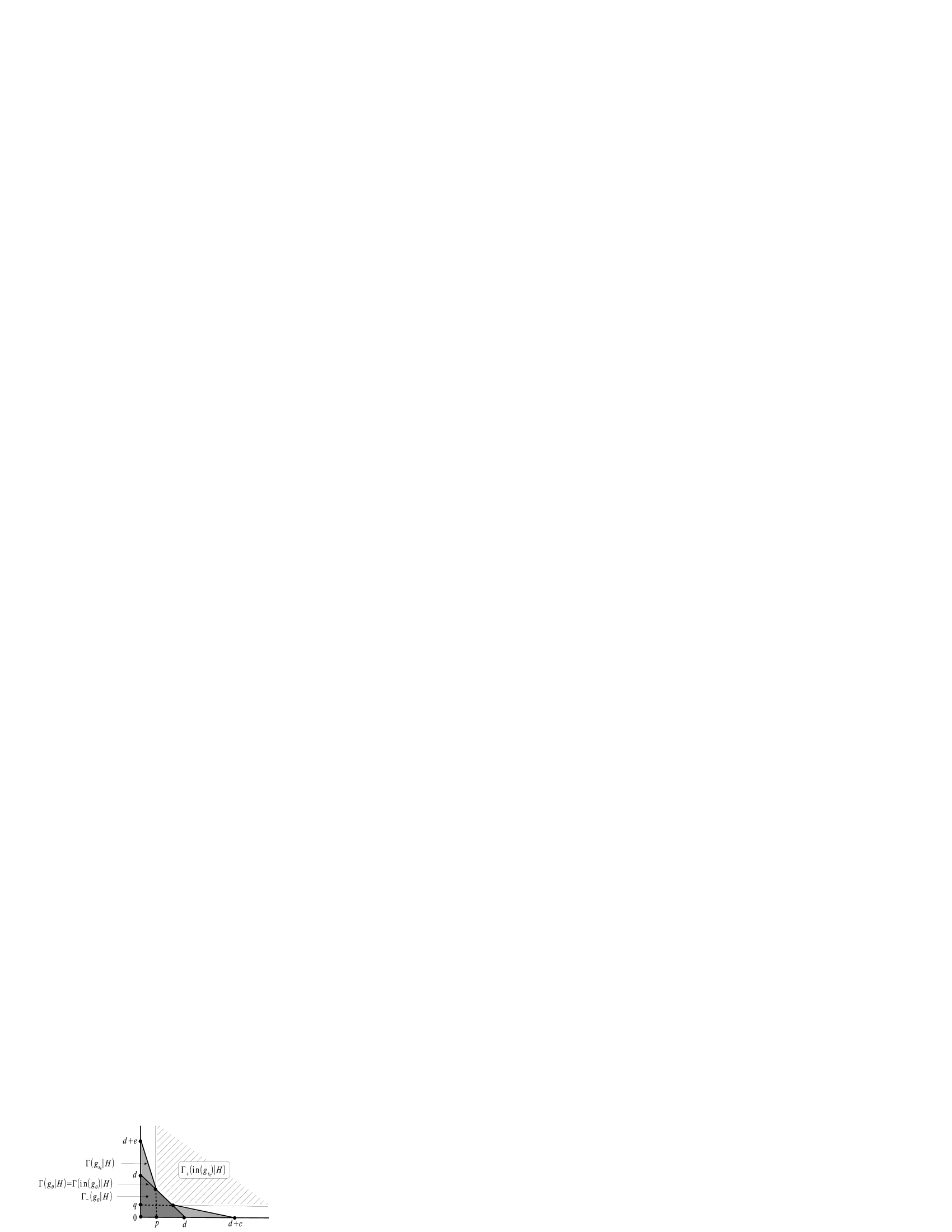
Figure 2. Newton boundaries and cones over them

Here, $\nu(\cdot)$ denotes the Newton number (see [7] for the definition) and $\Gamma_{\!-}(g_{s_{0}}|_{H})$ stands for the cone over $\Gamma(g_{s_{0}}|_{H})$ with the origin as vertex. (Again, $\Gamma(g_{s_{0}}|_{H})$ denotes the Newton boundary of $g_{s_{0}}|_{H}$ with respect to the coordinates $(x,y)$.) The polyhedron $\Gamma_{\!-}(g_{0}|_{H})$ is defined similarly. Since $\mu_{\mathbf{0}}(g_{s_{0}}|_{H})\geq\nu(\Gamma_{\!-}(g_{s_{0}}|_{H}))$ (see [7, Théorème 1.10]), altogether we have

$$\mu^{(2)}_{\mathbf{0}}(g_{s_{0}})=\mu_{\mathbf{0}}(g_{s_{0}}|_{H})\geq\nu(\Gamma_{\!-}(g_{s_{0}}|_{H}))>\nu(\Gamma_{\!-}(g_{0}|_{H}))=(d-1)^{2}=\mu^{(2)}_{\mathbf{0}}(g_{0}),$$

which is a contradiction to the $\mu^{*}$-constancy. ∎

Claim 5.4.

The zeta-function $\zeta_{g_{s},\mathbf{0}}(t)$ of the monodromy associated with the Milnor fibration of $g_{s}$ at $\mathbf{0}$ is independent of $s\in[0,1]$. In particular, the zeta-multiplicity $m_{\zeta}(g_{s})$ associated with the function $g_{s}$ and the zeta-multiplicity factor of $\zeta_{g_{s},\mathbf{0}}(t)$ are both independent of $s\in[0,1]$.

Proof.

This claim follows, for instance, from the following result of Teissier [18]: if $h$ and $h^{\prime}$ are two analytic functions such that $h(\mathbf{0})=h^{\prime}(\mathbf{0})=0$ and $h$ and $h^{\prime}$ can be connected by a $\mu^{*}$-constant piecewise complex-analytic path, then for any sufficiently small $\varepsilon>0$, the pairs

$$(S^{2n-1}_{\varepsilon},K_{h})\quad\mbox{and}\quad(S^{2n-1}_{\varepsilon},K_{h^{\prime}})$$

are diffeomorphic; here, $S^{2n-1}_{\varepsilon}$ stands for the sphere in $\mathbb{C}^{n}$ with centre $\mathbf{0}$ and radius $\varepsilon$, and $K_{h}$ denotes the link of $V(h):=h^{-1}(0)$, that is, $K_{h}:=S_{\varepsilon}^{2n-1}\cap V(h)$ for $\varepsilon>0$ small enough (of course, $K_{h^{\prime}}$ is defined similarly).

Alternatively, Claim 5.4 can also be deduced from [15, Lemma 12] which asserts that the independence with respect to $s$ of the Milnor number $\mu_{\mathbf{0}}(g_{s})$ implies the independence of the zeta-function $\zeta_{g_{s},\mathbf{0}}(t)$. This latter lemma follows from the Lê–Ramanujam theorem [11] together with the Sebastiani–Thom join theorem [17] and its generalization by Sakamoto [16] (for details, see [15]). ∎

Now, the expression for the zeta-function $\zeta_{g_{0},\mathbf{0}}(t)$ given by the formulas (2.15) and (2.16) shows that $m_{\zeta}(g_{0})\leq d$, but as observed above, we also have $m_{\zeta}(g_{0})\geq\mbox{mult}_{\mathbf{0}}(g_{0})=d$, so that altogether we get $m_{\zeta}(g_{0})=d$. Thus, by Claim 5.4, for any $s\in[0,1]$ we have $m_{\zeta}(g_{s})=d$. Moreover the zeta-multiplicity factor of $\zeta_{g_{s},\mathbf{0}}(t)$ satisfies the following property.

Claim 5.5.

For any $s\in[0,1]$, the zeta-multiplicity factor of $\zeta_{g_{s},\mathbf{0}}(t)$ is given by

$$(1-t^{d})^{c+\mu^{\mbox{\tiny\emph{tot}}}(C_{s})}$$

where $c$ is a constant independent of $s\in[0,1]$ and $\mu^{\mbox{\tiny\emph{tot}}}(C_{s})$ is the total Milnor number of $C_{s}$ (i.e., the sum of all local Milnor numbers associated with the singularities of $C_{s}$). In particular, since the zeta-multiplicity factor of $\zeta_{g_{s},\mathbf{0}}(t)$ is also independent of $s$ (see Claim 5.4), we have that $\mu^{\mbox{\tiny\emph{tot}}}(C_{s})$ is independent of $s$ as well.

Proof.

By a linear change of coordinates, we may assume that the initial polynomial $\mbox{in}(g_{s})$ is convenient and Newton non-degenerate on each coordinate subspace of dimension $2$ (i.e., $\mbox{in}(g_{s})|_{\mathbb{C}^{I}}$ is Newton non-degenerate for any $I\subseteq\{1,2,3\}$ with $|I|=2$). We may also assume that the singular points of $\mbox{in}(g_{s})$ are not located on the coordinate axes. Consider the regular simplicial cone subdivision $\Sigma^{*}$ of $W^{+}_{\mathbb{R}}$ whose vertices are the canonical weight vectors $\mathbf{e}_{1},\mathbf{e}_{2},\mathbf{e}_{3}$ together with the weight vector $\mathbf{w}:={}^{t}(1,1,1)$, and look at the associated toric modification $\hat{\pi}\colon X\to\mathbb{C}^{3}$, which is nothing but the ordinary point blowing-up with centre at the origin. The multiplicity of $\hat{g}_{s}:=\hat{\pi}^{*}g_{s}$ along the compact exceptional divisor $\hat{E}(\mathbf{w})\simeq\mathbb{P}^{2}$ is the degree $d$ of $\mbox{in}(g_{s})$. If the face function $(g_{s})_{\Delta(\mathbf{w};g_{s})}$ is not Newton non-degenerate, then the strict transform $\widetilde{V}$ of $V(g_{s})$ by $\hat{\pi}$ may have singularities in $\hat{E}(\mathbf{w})$. By Claim 5.3, $E(\mathbf{w})=\widetilde{V}\cap\hat{E}(\mathbf{w})$ (which is given by $\mbox{in}(g_{s})$) has only a finite number of isolated singularities $a_{1}(s),\ldots,a_{j_{s}}(s)$. To get a good resolution of $g_{s}$, we need further blowing-ups over these singular points. For each $1\leq j\leq j_{s}$, let $\hat{\omega}_{j}\colon Y_{j}\to X$ be the resolution with centre $a_{j}(s)$ which resolves $\hat{g}_{s}$ at $a_{j}(s)$. Denote by $\hat{\omega}\colon Y\to X$ the canonical gluing of the union (over all $1\leq j\leq j_{s}$) of these resolutions. Then

$$\hat{\Pi}:=\hat{\pi}\circ\hat{\omega}\colon Y\xrightarrow{\ \hat{\omega}\ }X\xrightarrow{\ \hat{\pi}\ }\mathbb{C}^{3}$$

gives a good resolution of $g_{s}$. The exceptional divisors of $\hat{\Pi}$ are the exceptional divisors $D_{1},\ldots,D_{r}$ of $\hat{\omega}$ and the pull back $\hat{E}_{Y}(\mathbf{w})$ of $\hat{E}(\mathbf{w})$ by $\hat{\omega}$. Now we observe that if $m_{i}$ denotes the multiplicity of $\hat{\Pi}^{*}g_{s}$ along $D_{i}$ ($1\leq i\leq r$), then, by Remark 2.1, $m_{i}$ is greater than the multiplicity $d$ of $\hat{\pi}^{*}g_{s}$ along $\hat{E}(\mathbf{w})$. We also notice that since $\hat{E}(\mathbf{w})\setminus\widetilde{V}$ is non-singular and does not contain any centre $a_{j}(s)$ ($1\leq j\leq j_{s}$), there is a canonical diffeomorphism

$$\hat{\omega}\colon\hat{E}_{Y}(\mathbf{w})\Bigg{\backslash}\Bigg{(}\widetilde{V}_{Y}\cup\bigcup_{1\leq j\leq r}D_{j}\Bigg{)}\overset{\sim}{\longrightarrow}\hat{E}(\mathbf{w})\setminus\widetilde{V},$$

where $\widetilde{V}_{Y}$ denotes the strict transform of $\widetilde{V}$ by $\hat{\omega}$. Altogether, this implies that the zeta-multiplicity factor of $\zeta_{g_{s},\mathbf{0}}(t)$ is given by

(5.3) $$(1-t^{d})^{-\chi(\hat{E}(\mathbf{w})\setminus\widetilde{V})}.$$

To show that $-\chi(\hat{E}(\mathbf{w})\setminus\widetilde{V})=c+\mu^{\mbox{\tiny tot}}(C_{s})$, where $c$ is a constant independent of $s$, we consider an analytic deformation $\{(g_{s})_{u}\}_{|u|<1}$ of $g_{s}$ obtained from a small perturbation of the coefficients of the face function $(g_{s})_{\Delta(\mathbf{w};g_{s})}$ such that $(g_{s})_{u}$ is Newton non-degenerate for all $u\not=0$ (as in §2.6). Then, for such a non-zero $u$, we have

$$\chi(\hat{E}(\mathbf{w})\cap\widetilde{V})=\chi(\hat{E}(\mathbf{w})\cap\widetilde{V((g_{s})_{u})})+\sum_{\mathbf{p}\in\mbox{\tiny Sing}(E(\mathbf{w}))}\mu_{\mathbf{p}}=\chi(\hat{E}(\mathbf{w})\cap\widetilde{V((g_{s})_{u})})+\mu^{\mbox{\tiny tot}}(C_{s}),$$

and hence,

$$\chi(\hat{E}(\mathbf{w})\setminus\widetilde{V})=\chi(\hat{E}(\mathbf{w})\setminus\widetilde{V((g_{s})_{u})})-\mu^{\mbox{\tiny tot}}(C_{s}),$$

where $\widetilde{V((g_{s})_{u})}$ is the strict transform of $V((g_{s})_{u}):=(g_{s})_{u}^{-1}(0)$. Of course,

$$\chi(\hat{E}(\mathbf{w})\setminus\widetilde{V((g_{s})_{u})})$$

is independent of $u\not=0$, but the key observation is that $\chi(\hat{E}(\mathbf{w})\setminus\widetilde{V((g_{s})_{u})})$ is also independent of $s\in[0,1]$ (remind that $\mbox{in}(g_{s})$ is convenient). This shows that the zeta-multiplicity factor of $\zeta_{g_{s},\mathbf{0}}(t)$ is written as

$$(1-t^{d})^{c+\mu^{\mbox{\tiny tot}}(C_{s})},$$

where $c:=-\chi(\hat{E}(\mathbf{w})\setminus\widetilde{V((g_{s})_{u})})$ is independent of $s\in[0,1]$ as desired. ∎

Remark 5.6.

Actually, the integer $c$ of Claim 5.5 is given by $c=d^{2}+3d-3$. Indeed, by Claim 5.4, we know that the zeta-multiplicity factor of $\zeta_{g_{s},\mathbf{0}}(t)$ is independent of $s$, so in order to prove the equality $c=d^{2}+3d-3$, it suffices to show that the zeta-multiplicity factor of $\zeta_{g_{0},\mathbf{0}}(t)$ is given by

$$(1-t^{d})^{d^{2}+3d-3+\mu^{\mbox{\tiny tot}}(C_{0})}.$$

By (2.14)–(2.16) and Remark 2.1, we easily see that the zeta-multiplicity factor of $\zeta_{g_{0},\mathbf{0}}(t)$ is written as

$$\zeta_{(g_{0})_{u}}(t)\cdot(1-t^{d})^{\mu^{\mbox{\tiny tot}}(C_{0})},$$

where $\{(g_{0})_{u}\}_{|u|<1}$ is a deformation of $g_{0}$ as above. But in our case the zeta-function $\zeta_{(g_{0})_{u}}(t)$ is nothing but $\zeta_{f_{0},\mathbf{0}}(t)$, which can be calculated using the Varchenko formula (2.7) as

$$\zeta_{(g_{0})_{u}}(t)=\zeta_{f_{0},\mathbf{0}}(t)=(1-t^{d})^{d^{2}+3d-3}.$$

We can now complete the proof of Theorem 5.1. For each $s\in[0,1]$, let again $a_{1}(s),\ldots,a_{j_{s}}(s)$ denote the singular points of $C_{s}$ and $\mu^{\mbox{\tiny tot}}(C_{s})$ denote the total Milnor number of $C_{s}$, that is, the sum of the local Milnor numbers $\mu(C_{s},a_{j}(s)):=\mu_{a_{j}(s)}(\mbox{in}(g_{s}))$ of the singularities $(C_{s},a_{j}(s))$ for $1\leq j\leq j_{s}$. Observe that if there is a bifurcation of the singularities at $s=s_{0}$ (for some $s_{0}\in[0,1]$) in a small ball $B_{j}$ centred at a singular point $a_{j}(s_{0})$ of $C_{s_{0}}$ — that is, $a_{j}(s_{0})$ is the only singular point of $C_{s_{0}}$ in $B_{j}$ and it is either a “newly born” singularity or a singularity obtained as a “merging” of several singularities of $C_{s}$ for $s$ near, but not equal to, $s_{0}$ (see Figure 3) — then, by [10, Théorème B] (see also [6, 8]), we have

$$\sum_{k=1}^{k_{j}(s)}\mu(C_{s},a_{j,k}(s))<\mu(C_{s_{0}},a_{j}(s_{0})),$$

where $a_{j,1}(s),\ldots,a_{j,k_{j}(s)}(s)$ are the singular points of the curve $C_{s}$ in the ball ${B}_{j}$. Let

$$Z:=\{(a,s)\in\mathbb{P}^{2}\times[0,1]\mid a\mbox{ is a singular point of }C_{s}\},$$

and let $\mbox{pr}_{1}\colon Z\to\mathbb{P}^{2}$ and $\mbox{pr}_{2}\colon Z\to[0,1]$ be the projections on the first and second factor respectively. Note that $\mbox{pr}_{1}(Z)=\bigcup_{s\in[0,1]}\{a_{1}(s),\ldots,a_{j_{s}}(s)\}$. By the above observation, if there is $s_{0}\in[0,1]$ such that $C_{s_{0}}$ gets either newly born singularities or several singularities of $C_{s}$ (for $s\not=s_{0}$ near $s_{0}$) merge into one (i.e., $s_{0}$ is a point where $\mbox{pr}_{2}$ fails to be a covering, see Figure 3), then we have $\mu^{\mbox{\tiny tot}}(C_{s})<\mu^{\mbox{\tiny tot}}(C_{s_{0}})$. However this contradicts Claim 5.5. Thus there is no such an $s_{0}$, and hence, by [9], the topological type of the pair $(\mathbb{P}^{2},C_{s})$ is independent of $s\in[0,1]$, so that $(C_{0},C_{1})$ is not a Zariski pair — a contradiction.

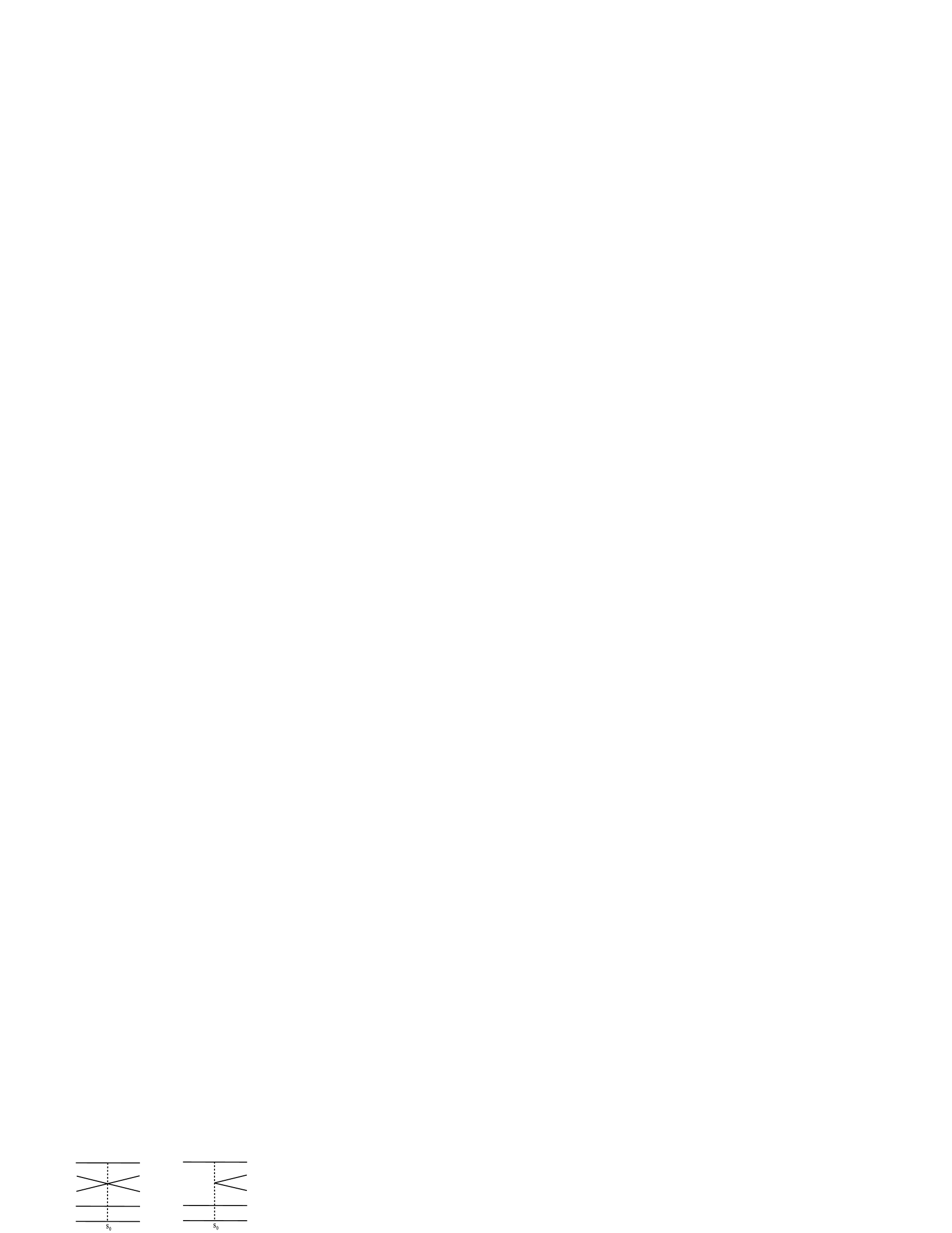
Figure 3. Bifurcation of singularities

This completes the proof of Theorem 5.1. ∎

Remark 5.7.

Theorem 5.1 remains valid if we assume that the pair of projective curves $(C_{0},C_{1})$ is only a weak Zariski pair instead of a Zariski pair. We recall that $(C_{0},C_{1})$ is said to be a weak Zariski pair if there is a bijection $\phi\colon\mbox{Sing}(C_{0})\to\mbox{Sing}(C_{1})$ between the singular loci $\mbox{Sing}(C_{0})$ and $\mbox{Sing}(C_{1})$ of $C_{0}$ and $C_{1}$, respectively, such that for any $p\in\mbox{Sing}(C_{0})$ the singularities $(C_{0},p)$ and $(C_{1},\phi(p))$ have the same embedded topological type (i.e., there are neighbourhoods $U_{p}$ and $U_{\phi(p)}$ of $p$ and $\phi(p)$, respectively, together with a homeomorphism of triples $\phi_{p}\colon(U_{p},C_{0}\cap U_{p},p)\to(U_{\phi(p)},C_{1}\cap U_{\phi(p)},\phi(p))$) while for any regular neighbourhoods $N(C_{0})$ and $N(C_{1})$ of $C_{0}$ and $C_{1}$, respectively, the pairs $(N(C_{0}),C_{0})$ and $(N(C_{1}),C_{1})$ are not homeomorphic (in particular, the pairs $(\mathbb{P}^{2},C_{0})$ and $(\mathbb{P}^{2},C_{1})$ are not homeomorphic either).

References

- [1] N. A’Campo, La fonction zêta d’une monodromie, Comment. Math. Helv. 50 (1975), 233–248.
- [2] V. I. Arnol’d, Normal forms of functions near degenerate critical points, the Weyl groups , , and Lagrangian singularities, Funkcional. Anal. i Priložen. 6 (1972), no. 4, 3–25.
- [3] E. Artal Bartolo, Sur les couples de Zariski, J. Algebraic Geom. 3 (1994), 223–247.
- [4] E. Artal Bartolo, J. I. Cogolludo, H. Tokunaga, A survey on Zariski pairs, in: Algebraic geometry in East Asia–Hanoi 2005, pp. 1–100, Adv. Stud. Pure Math. 50, Math. Soc. Japan, Tokyo, 2008.
- [5] M. Coste, Ensembles semi-algébriques, in: Real algebraic geometry and quadratic forms (Rennes, 1981), pp. 109–138, Lecture Notes in Math. 959, Springer, Berlin–New York, 1982.
- [6] C. Haş Bey, Sur l’irréductibilité de la monodromie locale; application à l’équisingularité, C. R. Acad. Sci. Paris Sér. A–B 275 (1972), A105–A107.
- [7] A. G. Kouchnirenko, Polyèdres de Newton et nombres de Milnor, Invent. Math. 32 (1976), 1–31.
- [8] F. Lazzeri, A theorem on the monodromy of isolated singularities, in: Singularités à Cargèse (Rencontre Singularités Géom. Anal., Inst. Études Sci. de Cargèse, 1972), pp. 269–275, Astérisque 7 & 8, Soc. Math. France, Paris, 1973.
- [9] Lê Dũng Tráng, Sur un critère d’équisingularité, C. R. Acad. Sci. Paris Sér. A-B 272 (1971), A138–A140.
- [10] Lê Dũng Tráng, Une application d’un théorème d’A’Campo à l’équisingularité, Nederl. Akad. Wetensch. Proc. Ser. A 76 = Indag. Math. 35 (1973), 403–409.
- [11] Lê Dũng Tráng and C. P. Ramanujam, The invariance of Milnor’s number implies the invariance of the topological type, Amer. J. Math. 98 (1976), no. 1, 67–78.
- [12] J. Milnor and P. Orlik, Isolated singularities defined by weighted homogeneous polynomials, Topology 9 (1970), 385–393.
- [13] M. Oka, Non-degenerate complete intersection singularity, Hermann, Paris, 1997.
- [14] M. Oka, Almost non-degenerate functions and a Zariski pair of links, arXiv:2105.03549, 2021.
- [15] M. Oka, On -Zariski pairs of links, arXiv:2203.10684, 2022.
- [16] K. Sakamoto, Milnor fiberings and their characteristic maps, Manifolds–Tokyo 1973 (Proc. Internat. Conf., Tokyo, 1973), pp. 145–150. Univ. Tokyo Press, Tokyo, 1975.
- [17] M. Sebastiani and R. Thom, Un résultat sur la monodromie, Invent. Math. 13 (1971), 90–96.
- [18] B. Teissier, The hunting of invariants in the geometry of discriminants, in: Real and complex singularities (Proc. Ninth Nordic Summer School/NAVF Sympos. Math., Oslo, 1976), pp. 565–678, Sijthoff and Noordhoff, Alphen aan den Rijn, 1977.
- [19] B. Teissier, Cycles évanescents, sections planes et conditions de Whitney, in: Singularités à Cargèse (Rencontre Singularités Géom. Anal., Inst. Études Sci., Cargèse, 1972), pp. 285–362, Astérisque 7 & 8, Soc. Math. France, Paris, 1973.
- [20] A. N. Varchenko, Zeta-function of monodromy and Newton’s diagram, Invent. Math. 37 (1976), no. 3, 253–262.
- [21] O. Zariski, On the problem of existence of algebraic functions of two variables possessing a given branched curve, Amer. J. Math. 51 (1929), no. 2, 305–328.
- [22] O. Zariski and P. Samuel, Commutative algebra, Vol. II, Reprint of the 1960 edition, Graduate Texts in Mathematics 29, Springer-Verlag, New York–Heidelberg, 1975.