Efficient and Automated Inversions of Magnetically-Sensitive Forbidden Coronal Lines: CLEDB - The Coronal Line Emission DataBase Magnetic Field Inversion Algorithm

1 Introduction

S-Introduction

Our need to measure the magnetic field threading the solar corona has never been more urgent. Society depends on electrical infrastructure in space and on the ground to an unprecedented and ever-increasing degree. The greatest single source of electrical perturbations on the Earth is the Sun, as has been known for at least a century and a half. Variable high energy radiation, ejection of magnetized plasma, the interactions of streams in adjacent sectors of the solar wind, all these lead to potentially dangerous effects on a technologically-dependent society. These and other issues are discussed in a variety of monographs, white papers and reviews (e.g. Billings, 1966; Judge et al., 2001; Eddy, 2009; Judge, Habbal, and Landi, 2013; Casini, White, and Judge, 2017; Ji et al., 2020).

The urgency of finding a reliable method to measure coronal magnetic fields arises from the fortunate conjunction of three unique observational opportunities. The Daniel K. Inouye Solar Telescope (DKIST, formerly ATST, see Rimmele et al., 2003, 2020), the Parker Solar Probe (PSP, formerly Solar Probe Plus, see Kinnison et al., 2013) and the Solar Orbiter mission (SolO, Marsch et al., 2005; Marsden, Müller, and StCyr, 2013) are all now operational. While the PSP and SolO orbit the Sun beyond 9 solar radii (R_⊙), sampling in-situ plasmas, neutral particles and magnetic fields, the 4 meter DKIST observatory will be able to measure components of magnetic fields at elongations $y\lesssim 1.5$ R_⊙. Such a large aperture, coronagraphic telescope operating from the peak of Haleakala marks a huge step up from early feasibility efforts with far smaller telescopes (e.g. Evans Solar Facility, SOLARC, COMP; Lin, Penn, and Tomczyk, 2000; Lin, Kuhn, and Coulter, 2004; Tomczyk et al., 2008). We also eagerly anticipate synoptic measurements with UCOMP (Tomczyk and Landi, 2019) and the 1.5 meter aperture coronagraph (www2.hao.ucar.edu/cosmo/large-coronagraph) of the COSMO suite of instruments, currently under review by the community.

In the current work, we describe a numerical method for studying magnetic signatures imprinted in the polarized light from magnetic dipole (M1) lines emitted at visible and infrared wavelengths by the corona. These M1 lines are formed in the saturated Hanle effect regime and are optically thin across the corona. Concerns have been expressed regarding line-of-sight (LOS) confusion (e.g. Judge, Habbal, and Landi, 2013; Schad and Dima, 2020). Mathematically, null spaces exist where variations in vector magnetic fields have no effect on the emergent spectra. Contributions to the familiar observed Stokes parameters $I,Q,U,$ and $V$ come from different regions along the LOS.

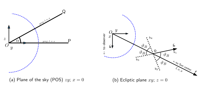
Figure 1.: Plane of sky and ecliptic plane geometry for coronal emitting structures. The blue dashed curve is the solar surface. The $y$- coordinate of the emitting plasma denotes the elongation. Panel (a) shows the geometry in the POS ($x=0$). Points $P$ and $Q$ see identical photospheric radiation from the Sun centered at $O$. The reference direction for linear polarization in the local vertical of the Sun [l.v.s.] is assumed throughout to be along the $z-$ axis. Panel (b) shows how points $b_{1},b_{2},b_{3}$ and $b_{4}$ along the vectors $\overrightarrow{ob_{1}},\overrightarrow{ob_{2}},\overrightarrow{ob_{3}},\overrightarrow{ob_{4}}$ experience the same value of $\cos^{2}\vartheta_{B}$, the angle between the local magnetic vector in the corona and the $l.v.s.$; the line joining the point to Sun center. At the angles traced along these dotted lines, and for the cones rotated about the $l.v.s.$, solutions of the statistical equilibrium equations are the same as for the solid line, that is when the saturated Hanle regime assumption holds. fig:sym

Single-point algorithms, like the one presented here must be considered a first step until stereoscopic observations, involving spacecraft in orbits significantly away from the Earth-Sun line of the corona, become available. Alternatively the Sun’s rotation might be used to try to probe the 3D coronal structure using stereoscopy (e.g. Kramar, Lin, and Tomczyk, 2016), assuming rigid coronal rotation over periods of days or longer. The corona may or may not comply with this assumption, and stationary structures which do comply may be of limited physical interest anyway.

Thus, our purpose is to present a method along with a python-based tool to allow coronal observers with DKIST and other telescope systems, to obtain a first estimate of properties of the emitting plasma including components of the vector magnetic field. Our primary simplification is

to seek solutions for the emitting plasma assuming it is dominated by one location along the line-of-sight.

For practical purposes, such “locations” make sense if they span LOS lengths smaller than, say, 0.1$R_{\odot}$. Naturally, without observations from a very different LOS in the solar system, the measurements represent differently-weighted averages of physical conditions along each LOS. These solutions inherently possess well-known ambiguities arising from specific symmetries associated with the line formation problem, as shown for example in Figure fig:sym. Therefore, our inversion scheme allows one to identify, but not necessarily resolve, all ambiguities from a set of observed Stokes profiles, as revealed in Section S-CLEDB. Section S-discussion provides a summary of the findings, and discusses multiple emission locations as suggested by multiple components in the emission lines, where solutions for each can, in principle, be obtained.

2 Review of the Formation of Forbidden Coronal Lines

S-formalism

2.1 Emission Coefficients in Statistical Equilibrium

We adopt the formalism and notation of Casini and Judge (1999), that expands upon earlier work on loosely related topics (e.g. Sahal-Brechot, 1977; Landi Degl’Innocenti, Bommier, and Sahal-Brechot, 1991; Landi Degl’Innocenti, 1982). We must solve for the magnetic substate populations of the radiating ions assuming statistical equilibrium (SE). The problem is cast into the framework of spherical tensors to take advantage of geometrical symmetries (see Chapter 3 in Landi Degl’Innocenti and Landolfi, 2004). Magnetic Dipole (M1) coronal lines form under regimes where Zeeman frequency splittings are of order of the classical Larmor frequency $\nu_{L}$, $h\nu_{L}=\mu_{0}\cdot B$ and are far smaller than the Doppler widths $\Delta\nu_{D}$, and where the Einstein - A coefficients $A_{JJ_{0}}$ are, in turn $\ll\nu_{L}$. The first inequality permits an accurate Taylor expansion of line profiles in terms of the small quantity $\delta=\nu_{L}/\Delta\nu_{D}\ll 1$ (Casini and Judge, 1999). The second defines the “strong-field limit of the Hanle effect” in which coherences between magnetic sub-states of the decaying level are negligible in the magnetic-field reference frame. From the solutions to the SE equations, the emission coefficients for the Stokes vector $(S_{0},S_{1},S_{2},S_{3})^{T}$ $\equiv(I,Q,U,V)^{T}$ are then (see Equations 35a-35c in Casini and Judge (1999)):

$$\varepsilon_{0}^{(0)}(\nu,\hat{\bf k}) = \epsilon_{JJ_{0}}\,\phi(\nu_{0}-\nu)\left[1+D_{JJ_{0}}\,\sigma^{2}_{0}(J)\,{\cal T}^{2}_{0}(0,\hat{\bf k})\right]\;,$$ (1)

$$\varepsilon_{i}^{(0)}(\nu,\hat{\bf k}) = \epsilon_{JJ_{0}}\,\phi(\nu_{0}-\nu)\,D_{JJ_{0}}\,\sigma^{2}_{0}(J)\,{\cal T}^{2}_{0}(i,\hat{\bf k})\;,\qquad(i=1,2)$$ (2)

$$\varepsilon_{3}^{(1)}(\nu,\hat{\bf k}) = -{\textstyle\sqrt{\frac{2}{3}}}\,\nu_{\rm L}\,\epsilon_{JJ_{0}}\,\phi^{\prime}(\nu_{0}-\nu)\left[\bar{g}_{J,J_{0}}+E_{JJ_{0}}\,\sigma^{2}_{0}(J)\right]{\cal T}^{1}_{0}(3,\hat{\bf k})\;,$$ (3)

where the M1 transition occurs from level with angular momentum $J$ to $J_{0}$, and where

$$\epsilon_{JJ_{0}}={\frac{h\nu}{4\pi}}\,N_{J}\,A_{JJ_{0}}.$$ (4)

$\phi(\nu_{0}-\nu)$ is the (field-free) line profile (in units of Hz^-1), with $\int_{0}^{\infty}\phi(\nu_{0}-\nu)d\nu=1$ and $\phi^{\prime}(\nu_{0}-\nu)$ denotes its first derivative with respect to $\nu$.

When integrated along a specific LOS, the expressions for the emission coefficient $\varepsilon^{(i)}_{i}(\nu,\hat{\bf k})$, with units of erg cm^-3 sr^-1s^-1, yield the emergent Stokes vectors from the corona. $\epsilon_{JJ_{0}}$ is the usual coefficient for the frequency-integrated isotropic emission only from the line, ignoring stimulated emission, where the $D_{JJ_{0}}$ and $E_{JJ_{0}}$ coefficients are dimensionless parameters associated with the polarizability of the two atomic levels.

The superscripts on $\varepsilon^{i}$ are the leading orders in the Taylor expansion of the line profile

$$\phi(x+dx)=\phi(x)+\sum_{j=1,...}\frac{d^{j}}{dx^{j}}\phi(x)\cdot dx^{j}\ldots$$ (5)

with $dx\propto\delta=\nu_{L}/\Delta\nu_{D}\ll 1$. Second order terms in $\delta$ are negligible for weak coronal fields and broad line profiles. Lastly, here it is assumed that the photospheric radiation is spectrally flat across the corona line profiles (Casini and Judge, 1999).

2.2 Physical Interpretation

These equations are readily understood physically. The leading order in the $IQU$ Stokes signals is zero, for Stokes $V$ it is one. $IQ$ and $U$ arise from a combination of thermal emission and scattering of photospheric radiation, both include the populations $N_{J}$ and the atomic alignment $\sigma^{2}_{0}(J)$. Both quantify local solutions to the SE equations, entirely equivalent to solving for populations of magnetic sub-states (House, 1977; Sahal-Brechot, 1977). Alignment is generated entirely by the anisotropic irradiation of ions by the underlying solar photospheric radiation. Information on the magnetic field in $IQU$ is contained implicitly in $\sigma^{2}_{0}(J)$ and is independent of magnetic field strength, as corresponding to the mathematical statement of the strong field limit. In contrast, Stokes $V$ for the M1 lines is formed entirely through the Zeeman effect, modified by the alignment factor (Casini and Judge, 1999). When the atomic alignment factor is zero, the expression for Stokes V reduces to the well-known “magnetograph formula” of the Zeeman effect, to first order. The leading terms for $QU$ in the Zeeman effect are only second order in $\delta$ leading them to be considered negligible in coronal cases due to small B magnitudes. Together with the first order term in $V$ they form the basis of most solar “vector polarimeters” (e.g. Lites, 2000).

The coefficients $D_{JJ_{0}}$, $E_{JJ_{0}}$ are properties fixed by quantum numbers $J$ and $J_{0}$ of the two atomic levels. f $D_{JJ_{0}}$ is fixed by $J$ and $J_{0}$, but $E_{JJ_{0}}$ also depends on each level’s “Landé g-factor” that are used to build “effective Landé factors” of the transition, $\bar{g}_{J,J_{0}}$. The Landé g-factors also depends on quantum numbers other than $J,J_{0}$, like the mixing of atomic states and orbital and spin angular momenta. These can be measured or may be computed using an atomic structure calculation. See, for example, new calculations of special relevance to this work by Schiffmann et al. (2021).

The Taylor expansion of $\varepsilon_{i}^{(o)}(\nu,\hat{\mathbf{k}})$ with frequency has leading orders $o=1$ when $i=3$ and $o=0$ otherwise (Casini and Judge, 1999).

The terms $N_{J}$ and $\sigma^{2}_{0}(J)$, the population and alignment of level with total angular momentum $J$, are solutions to SEs. These solutions, which are linear combinations of the populations of magnetic substates of level $J$ (e.g., Sahal-Brechot, 1977), depend both on the scattering geometry, the magnetic unit vector $\hat{\mathbf{b}}$, and the plasma temperature and density. The atomic alignment $\sigma^{2}_{0}(J)$ is created by the bright, anisotropic photospheric cone of radiation seen by the coronal ions, and destroyed by collisions with plasma particles having isotropic distributions. This “atomic polarization” is modified by the magnetic field as the ion’s magnetic moment precesses around the local B-field. The appearance of $\sigma^{2}_{0}(J)$ in the SE equations underlying Equations eqn:eps00-eqn:eps31 show that linearly polarized light in the corona originates from atomic polarization, and also that the intensity and Zeeman-induced circular polarization are modified by it.

2.3 Scattering Geometry

Finally, the spherical tensors ${\cal T}^{K}_{0}(i,\hat{\bf k})$ define the geometry of the scattering of solar radiation for Stokes component $i$ from the coronal plasma. The tensors play no role in the SE calculations, as is readily appreciated, in that the SE states cannot depend on the observer. Figure fig:sym(b) shows instead how the solutions depend on $\vartheta_{B}$, the angle between the local magnetic field and the radius vector $\hat{\mathbf{r}}$ to the local vertical of the Sun (l.v.s).

3 CLEDB, a Database Approach for “Single-Point Inversions”

S-CLEDB

3.1 The CLEDB Algorithm

Figure 2.: A simplified view of the CLEDB module scheme. Three modules each focus on: the database generation via CLEDB_BUILD; the CLEDB_PREPINV data pre-processing; and the CLEDB_PROC data analysis and inversion. The CLEDB_BUILD module requires the execution of precompiled Fortran binaries of the CLE code due to computation speed requirements. Ideally, databases are only generated once per system based on user requirements. The other two modules are based on Python. The data analysis is split into two branches with different output products based on wether 1-line or 2-line Stokes IQUV data is ingested. An in-depth module description can be found in the documentation linked in the data availability section.fig:flowcledb

The Coronal Line Emission DataBase (CLEDB) inversion algorithm is created to harness all available information in polarization measurements of the corona to infer local plasma properties and vector magnetic fields. A non-commercial open-source python-based code package of CLEDB, designed for both personal computer jobs and SLURM (Simple Linux Utility for Resource Management) enabled research computing jobs, is freely available online. More information about the code, package, and method documentation along with persistent links are found in the data availability section. The algorithm uses the equations and framework described in Section S-formalism together with symmetries and line profile properties to extract magnetic and thermal information from measured Stokes parameters through a search of a database of computed Stokes parameters.

A single emission line does not contain sufficient information for a full inversion. This will become clear below, but see Plowman (2014), Dima and Schad (2020), and Judge, Casini, and Paraschiv (2021) for detailed discussions. Therefore, the CLEDB approach is primarily designed for two or more coronal lines. A secondary code branch will be used to derive basic thermal parameters and LOS magnetic fields only, when Stokes observations of 1-line are provided instead of 2-line using analytical approximations incrementally developed by Casini and Judge (1999), Plowman (2014) and Dima and Schad (2020).

In the CLEDB 2-line configuration, solutions that are deemed a good fit, currently by using a reduced $\chi^{2}$ metric, are returned along with database model magnetic, geometric and thermal parameters as acceptable solutions to the inverse problem.

The algorithm seeks thermal and magnetic conditions from a single point along the LOS. This is a gross oversimplification in general, but it is well known that coronal images frequently reveal discrete structures, such as in polar plumes or more especially in loops over magnetically active regions. These are the regions of great interest for space weather disturbances at the Earth (Ji et al., 2020). However, in cases such as the quiet Sun, the emission is distributed diffusely and our method will represent some poorly-defined average of quantities along the LOS. We explore this assumption below. In essence, we replace the integrals of equations eqn:eps00-eqn:eps31 over the LOS with a 1-point quadrature using a length scale $\ell$. For convenience, we choose $\ell=1$ and use henceforth,

$$\ilabel{eq:S}S_{i}(\nu,\hat{\mathbf{k}})\equiv\epsilon_{i}^{(o)}(\nu,\hat{\mathbf{k}}),$$ (6)

which is the emergent Stokes parameter of the emission line for a path length of 1 cm along $\hat{\mathbf{k}}$.

Even with this simplification, there is always some ambiguity in the solutions owing to inherent symmetries. Our algorithm therefore returns all such solutions deemed to be compatible with the data.

Angle	definition	source	notes
$\alpha$	arctan$(z/y)$	this work	Figure 1(a)
$\phi$	$\arccos\left(\mathbf{\hat{x}\cdot(\hat{b}\times\hat{z})}\right)$	this work	azimuthal angle of $\mathbf{B}$
$\theta$	arccos$(\mathbf{\hat{z}\cdot\hat{b}})$	this work	polar angle of $\mathbf{B}$
$\vartheta$	arccos$(\hat{\mathbf{k}}\cdot\hat{\mathbf{r}})$	CJ99 fig. 5	(angle between LOS and l.v.s.)
$\vartheta_{B}$	$\arccos(\mathbf{\hat{r}\cdot\hat{b}})$	CJ99 fig. 5	(See also Figure 1(b))
$\varphi_{B}$	$\arccos\left(\mathbf{(\hat{k}\times\hat{r})\cdot(\hat{b}\times\hat{r})}\right)$	CJ99 fig. 5
$\Theta_{B}$	arccos$(\mathbf{\hat{k}\cdot\hat{b}})^{\ast}$	CJ99 fig. 5
$\Phi_{B}$	$\frac{1}{2}\arctan(U/Q)$	CJ99 fig. 5

Table 1.: Angle definitions in the l.v.s frame except where noted

^∗As observed from Earth, the LOS and $x$- axis are almost parallel. For example an elongation $\sqrt{y^{2}+z^{2}}$ of $2R_{\odot}$ the angle between the LOS and $\hat{\mathbf{k}}$ is only has $0.0093$ radians (0.5^o). Any errors introduced with this assumption are minor compared with the other observational and theoretical challenges presented by the problem at hand. tab:angles

3.2 Frames of Reference

Figures fig:sym, fig:spheresm and Table tab:angles define various angles in terms of a Cartesian reference frame with its origin at the center of the Sun. The axes $\mathbf{\hat{x}},\mathbf{\hat{y}},\mathbf{\hat{z}}$ point along the Sun center-observer line, the E-W direction and S-N direction relative to the Sun’s rotational axis in the plane-of-the-sky. We adopt the reference direction for linear polarization to be along the $z$- axis (vertical). This corresponds to the direction of a linear polarizer measuring $\frac{1}{2}(I+Q)$ (see p. 19 of Landi Degl’Innocenti and Landolfi, 2004).

Two unit vectors $\hat{\mathbf{r}}$ and $\hat{\mathbf{b}}$ specify the direction of the center of the cone of photospheric radiation and magnetic field, and a third $\hat{\mathbf{k}}$ specifies the LOS.

We define two reference frames, the “solar” frame and the “observer” frame. All angles in the solar frame are specified as Greek lowercase letters. Two more angles are defined in uppercase, defined relative to the observer. $\Theta_{B}$ is the angle between the LOS vector $\hat{\mathbf{k}}$ and $\hat{\mathbf{b}}$. The angle $\Phi_{B}$ follows from our adoption of a reference direction parallel to the $\hat{\mathbf{z}}$- axis. With this geometry,

$$\ilabel{eq:Phib}\Phi_{B}=\pi-\gamma_{B}=+\frac{1}{2}\arctan\frac{U}{Q}$$ (7)

for each line with measurable $Q$ and $U$.

Table 2.: 2-line CLEDB solution output products compared with synthetic observations.

The CLEDB solutions are degenerate to 180^∘ with respect to the LOS angle components. The CLE atmosphere parameters provide the ground-truth reference values. These are averaged along the LOS. H and D refer, respectively, to the coronal height above the limb and the LOS depth in units of R_⊙. The electron density is given in $\log 10$ cm^-3, magnetic angles in degrees, and magnetic field components in G. tab:table1 Index $\chi^{2}$ n_e H D $|$B$|$ $\Phi_{B}$ $\Theta_{B}$ B_x B_y B_z 5982696 2.12e-2 8.10 1.18 -0.52 6.0 108.3 72.8 -1.85 5.47 1.72 6669594 2.12e-2 8.05 1.18 0.55 6.0 253.3 108.9 -1.63 -5.47 -1.93 5990814 2.13e-2 8.10 1.18 -0.52 -6.0 289.4 108.9 -1.93 5.47 1.93 6661476 2.13e-2 8.05 1.18 0.55 -6.0 72.2 72.8 -1.71 -5.52 -1.72 5982606 3.65e-2 8.10 1.18 -0.52 6.8 106.6 72.8 -1.88 6.28 2.02 6669684 3.65e-2 8.05 1.18 0.55 6.8 255.0 108.9 -1.68 -6.28 -2.29 5982697 5.64e-2 8.10 1.18 -0.52 5.9 108.3 74.5 -1.81 5.44 1.57 6669593 5.64e-2 8.05 1.18 0.55 5.9 253.3 107.1 -1.61 -5.44 -1.74 5990904 5.79e-2 8.10 1.18 -0.52 -5.4 291.2 108.9 -1.94 4.89 1.84 6661386 5.79e-2 8.05 1.18 0.55 -5.4 69.9 72.8 -1.75 -4.91 -1.60 CLE : 7.97 1.18 -0.49 6.3 -1.59 5.72 2.02

3.3 Symmetries to Minimize Numerical Work

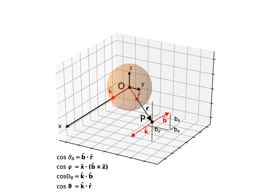
Figure 3.: The scattering geometry of point $P$ is shown in the observer’s frame with projections of the magnetic field components in the same frame. The LOS through Sun center lies along unit vector $\mathbf{\hat{k}}$, which is parallel to the $x$-axis. We assume that the LOS through the corona are parallel to $\mathbf{\hat{k}}$. $\Phi_{B}$ ($=\pi-\gamma_{B}$ in CJ99) is defined by $\arctan\hat{b}_{z}/\hat{b}_{y}$ if we take the reference direction for linear polarization along the $z$- axis. The unit vectors of interest are marked with red arrows. fig:spheresm

Frequency-dependent line profiles are not required because we know a priori that, under the single-point contribution assumption, the profiles for $I,Q,U$ are identical, namely the zeroth-order term in the Taylor expansion. The leading order in the $V$ profile is the first order term $\propto dI/d\nu$. Therefore we need only create a database of quantities $\varepsilon^{(i)}(\nu,\hat{\mathbf{k}})$ appropriately integrated over frequency,

$$\ilabel{eq:si}S_{i}=\int_{\mathrm{line}}[I(i,\lambda)-I(i,\lambda_{c})]\;d\lambda.$$ (8)

The integration for an observed set of Stokes $O_{i}$ follows the same formalism, when subtracting $\lambda_{c}$ continuum emission and setting any Doppler shifts to zero. The integral for $V$ requires weights of opposite sign at either side of the line center. If two or more components are identifiable in the $I(\nu,\hat{\mathbf{k}})$ profiles, for example by multiple fits of Gaussian profiles, the components can be extracted beforehand, and searches made for each component.

Even with these simplifications, minimal implementations of a search algorithm would generate databases of impractically large sizes. A 3D Cartesian grid built around a quadrant around the solar disk (Figure fig:spheresm), would demand computation of the $S_{i}$ parameters at each of, say, $50\times 50\times 50$ “voxels”. Each such voxel requires a grid of magnetic vectors $\mathbf{B}=(B_{x},B_{y},B_{z})^{T}$, the LOS components of velocity field $v_{x}$, temperature $T$, density $n_{e}$, elemental abundance $\mathcal{A}$, and a spectroscopic turbulence representing unresolved non-thermal motions $v_{T}$. With over $10^{5}$ voxels, the number of database entries would exceed $N_{C}\geq 10^{13}$, using just 10 values for each of the magnetic and thermodynamic variables listed above. But the database size can be dramatically reduced based upon the following arguments:

1. Observations are subject to the geometrical rotation of the $Q$ and $U$ profiles using equations eq:qrot and eq:urot. All $QU$ data can be rotated around the $x$-axis by the azimuth angle $-\alpha$, as shown in Figure fig:sym(a). Database searches can then be limited to those LOS within the $z=0$ plane instead of the entire 3D volume; e.g. point Q is different from point P in Figure fig:sym(a) only by the $\alpha$-rotation of the Q and U Stokes profiles. Afterwards, matching magnetic vectors are simply rotated back by $+\alpha$. The $I$ and $V$ Stokes parameters are invariant to rotations about the LOS ($x$- axis).

2. We need only to search along the LOS $x$- direction using $n_{y}$ separately stored database files for each observation with an observed elongation $y$ closest to the computed CLEDB height $y_{0}$, minimizing CPU and memory requirements.

3. We suggest adopting line pairs from a single ion, eliminating the need to account for relative abundances and differential temperatures along each LOS. However, it is possible to use different ions, even of different elements, although this is not advisable for reasons that will become clear below. (see Judge, Casini, and Paraschiv (2021) for detailed discussions.)

4. We can compute the Stokes parameters and store them for a single field strength $B=|{\mathbf{B}}|$. We then compute the ratio between the computed and the observed values of circular polarization. This simplification results from the strong field limit of the Hanle effect. In other words, CLEDB will solve for the geometry, thermal, and magnetic orientation, and afterwards scale the magnetic field strength using Zeeman diagnostics (equation eqn:eps31).

Thus, in this example, the CLEDB scheme’s database will encompass $N_{C}\approx 10^{6}$ entries for each of the $n_{y}$ database computed elongations, as shown in Table tab:discretization. The numbers quoted in this example are not absolute and represent just a starting point. In CLEDB the database parameter configuration is a user editable feature when building databases within the CLEDB_BUILD module.

The first simplification is equivalent to a rotation of our choice of reference direction for linear polarization. The $Q$ and $U$ parameters fed to the search algorithm are simply

eq:qrot$$Q_{\alpha} = Q\cos 2\alpha-U\sin 2\alpha,$$ (9)

$$U_{\alpha} = Q\sin 2\alpha+U\cos 2\alpha.$$ (10)

The preference for lines belonging to single ions described in Point 3 is not a serious restriction, because ions of the $np^{2}$ and $np^{4}$ iso-electronic sequences with $n=2$ and $n=3$, such as Fe XIII, possess two M1 lines in the ${}^{3}P$ ground terms whose dependencies of $\varepsilon_{i}^{(o)}(\nu,\hat{\bf k})$ on electron temperature are essentially identical, determined by collisional ionization equilibrium. The Fe XIII 1.0747 $\mu$m and 1.0798 $\mu$m line pair has served as the primary target for previous instruments (Querfeld, 1977; Tomczyk et al., 2008), and remains a prime candidate for new observations with DKIST. Point 4 entails the significant benefit of finding solutions which depend on higher signal wavelength-integrated Stokes profiles (equation eq:si), rather than noisier differences, of Stokes $V$ profiles (cf. Equation 11 of Dima and Schad, 2020). We note that the accuracy of database vs. observation scaling is dependent on LOS effects that are not currently fully quantified, as can be seen in the $\chi^{2}$ values of Table tab:table1 that indicate overfitting.

Figure 4.: CLEDB 2-line magnetic inversion algorithm flowchart that is a subcomponent of the CLEDB_PROC module. An important aspect is the delivery of multiple possible solutions for each observation at the last step. Note that the $x$- coordinate of the point in space, as well as nearest electron density, are returned along with $\mathbf{B}$. The figure uses the notation $V_{\mathrm{obs}}$ and $V_{\mathrm{db}}$ for observed and computed values of the amplitudes of the Stokes parameters corresponding to $O_{3}$ and $S_{3}(B=1)$ in the text. fig:flow

The search over angles can then be further restricted. We use the ratio $U_{\alpha}/Q_{\alpha}$ to estimate the azimuth angle $\Phi_{B}$ modulo $\pi/2$ for every M1 line (see Figure fig:sym). In the database we adopt grids for the magnetic field vector in spherical coordinates at the point $P$ for angles $\phi$ and $\theta$ in Table fig:spheresm. For each $\Phi_{B}$, the $\phi$ and $\theta$ angles are related by their definitions by:

$$\ilabel{eq:qu}\tan\Phi_{B}=\tan\theta\sin\phi.$$ (11)

Ultimately we are left only to search a 4-dimensional discretized hyperspace for each elongation $y$, to identify matching values of $n_{e}$, $x$, $\phi$, and $\bar{\theta}(\phi)$ remembering that B is scaled afterwards, as discussed above. Here $\bar{\theta}(\phi)$ includes only values of $\theta$ compatible with equation eq:qu.

In our Table tab:table1 example of CLEDB sorting, we simply presort the 10 values of $\bar{\theta}$ in the numerical grid that are most compatible with Equation eq:qu. We see that solutions are degenerate in pairs of two in terms of supplementary $\Phi_{B}$ and complementary $\Theta_{B}$ angles. The number of presorted $\bar{\theta}$ solutions is configurable via CLEDB controlling parameters. Interpolation is of course possible, but it is not currently implemented due to the yet unknown effects of potential uncertainties.

Yet more computational savings are made noting that the electron densities $n_{e}$ are strong functions of $r$ because of stratification and solar wind expansion. Thus, we can reasonably seek solutions of a fixed analytical form for $n_{e}(r)$ as shown in Table tab:discretization. The function

$$n_{0}(r)=3\cdot 10^{8}\cdot\exp\left(-\frac{r-1}{h}\right)+10^{8}\cdot(0.036r^{-3/2}+1.55r^{-6}),$$ (12)

has $r$ in units of $R_{\odot}$, and scale height $h=0.0718R_{\odot}$ ($\equiv$ 50 Mm), where the second term is the formula of Baumbach (Allen, 1973). The grid-sizes that we have used for testing, and we consider a reasonable starting point are given in Table tab:discretization. The resulting density is given by a smaller array of say 15 discretized values centered on the base $n_{o}$ electron density, which span orders of magnitude of -2 to 2 in logscale.

quantity	number	range
$\log_{10}n_{e}/n_{0}^{\dagger}(r)$ (electron density)	$n_{n_{e}}=15$	$-2\rightarrow+2$
$x$- axis (LOS, units $R_{\odot}$)	$n_{x}=100$	$-2.5\to 2.5$
$\phi$	$n_{\phi}$ = 180	$0\to 2\pi$
$\theta$	$n_{\theta}$ = 90	$0\to\pi$
$\bar{\theta}$	$n_{\bar{\theta}}\approx 10$	$0\to\pi$
$N=n_{n_{e}}n_{x}n_{\phi}n_{\theta}$	24.3 million
$N^{\prime}=n_{n_{e}}n_{x}n_{\phi}n_{\bar{\theta}}$	2.7 million
Size of each database file of 2 lines, each with	388 MB
4 Stokes parameters stored as 32 bit integers

Table 3.: Example of numerical discretization for each database file at elongation $y_{0}$.

The $N$ and $N^{\prime}$ represent the sizes of databases as computed with either $n_{\theta}$ or $n_{\bar{\theta}}$. These correspond respectively to all database orientations and to the subset compatible with equation eq:qu. Each of the two discretization options can be user-selected via CLEDB control parameters. tab:discretization

We used the reduced $\chi^{2}$ metric as a goodness of fit, with Stokes ‘observations’ $S_{i}$ taken from values on the database grid. Then we write $\chi^{2}$ as the sum of

eq:chisq$$\chi^{2}_{\text{\tiny IQU}}= \dfrac{1}{d-p} \left[\sum_{i=0,1,2}{\frac{(S_{i}-O_{i})^{2}}{\sigma^{2}_{i}}}\right]\text{ and}$$ (13)

$$\chi^{2}_{\text{\tiny V}}= \dfrac{1}{d-p} \frac{(S_{3}-O_{3})^{2}}{\sigma^{2}_{3}}$$ (14)

where $O_{i}$ and $\sigma_{i}$ are for the observed Stokes $I,Q,U$ parameters, and $O_{3}$ and $\sigma_{3}$ correspond to Stokes $V$. Here $\sigma^{2}$ is a variance associated with noise, not to be confused with the alignment $\sigma^{2}_{0}(J)$ which always is specified by $J$. The distribution of noise in $O_{i}$ is normal with standard deviation $\sigma_{i}$. The rms noise is added to $\sigma_{i}$ as a function of the number of photons detected in the line. We normalize the set of 8 Stokes parameters with respect to the Stokes $I$ parameter corresponding to the strongest line in the set, in order to bypass the need for absolute intensity calibrations. Here, $d=4\,n_{line}-1$ is the number of independent data points. The number of free parameters in the model is $p=4$. With $d=7$ for two lines, the factor $(d-p)^{-1}$ in Equation eq:chisq is $\frac{1}{3}$, and the sum would be over two lines.

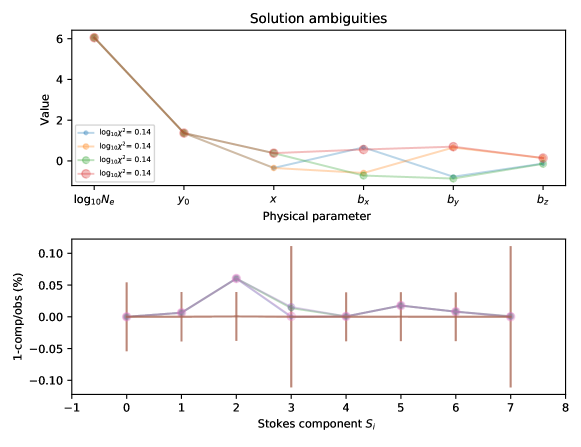
Figure 5.: The figure shows four solutions computed by the database search algorithm that are compatible ($\chi^{2}<1.4$) with synthetic Stokes components of both the Fe XIIII 1.0474 $\mu$m and 1.0798 $\mu$m lines. The synthetic data are for a randomly chosen model calculation with statistical errors from 63 million counts in the 1.0747 $\mu$m line. The lower panel shows the differences in percent of the Stokes parameters in the observations, associated error bars, and solutions found from the search algorithm.fig:amba

The reasoning behind separating the first three and last Stokes parameters in Equations eq:chisq and eq:chisq2 comes from the strong-field limit of the Hanle effect. As already described, the first three Stokes parameters $IQU$ depend only on the direction (e.g. unit vector $\hat{\mathbf{b}}$), and not the magnitude $B$ of the magnetic field. On the other hand, Stokes $V$ parameters scale only with the magnitude $B$ of the magnetic field. Thus, the $\chi^{2}$ sorting needs to be separated into its two components, as shown in Equations eq:chisq-eq:chisq2. We store in the database Stokes vectors $S_{i}$ computed only with $B=1$ G. The first 3 Stokes parameters, are determined by minimization of Equation eq:chisq yielding acceptable values of $\hat{\mathbf{b}}$, along with the smallest normed differences in integrated Stokes $V$, as given by a database search. Once the direction $\hat{\bf b}$ is known, the contribution of Stokes $V$ to $\chi^{2}$ in Equation eq:chisq2 is identically zero only when

$$S_{3} = O_{3},\mathrm{\ \ hence}$$

$$B = O_{3}/S_{3}(B=1),$$ (15)

which is the analytical solution for $B$ because $S_{3}=B\cdot S_{3}$, where $B=1$.

Equation eq:algebraic then yields the magnetic field strength compatible with all the observed and computed Stokes parameters, without reference to the values $\sigma_{3}$ for each line. The value of $V$ used for estimating $B$ can be taken either from the strongest line or the weighted mean of a number of observed lines via a CLEDB configuration parameter. This procedure justifies argument number 4 listed above.

To sum up, the number of calculations needed becomes of the order of $10^{6}$ when using the discretization example in Table tab:discretization, so that searches become fully tractable even on desktop computers. Figures fig:flowcledb and fig:flow show the overview and detailed CLEDB scheme as flowcharts.

3.4 Performance

In some initial tests using Python, solutions are obtained in 0.2 sec. for the parameters listed in Table tab:discretization, using a fairly current off-the-shelf laptop like a 64-bit Macbook Pro with a 2.3 GHz Quad-Core Intel Core i7, with 16GB RAM. By compressing database files storage to 32 bit integers, we halve the disk space required, while incurring about 2 sec. of overhead each time the data are read and decompressed. There is therefore a small advantage in finding all observations matching a given database value of $y_{0}$ before searching for solutions. CLEDB implements such a pre-search in its CLEDB_PREPINV module, where for any measured cluster of $y$- heights, CLEDB searches and selects the nearest $y_{0}$ database position.

Figure 6.: The number of solutions $\chi^{2}<1.4$ compatible with a randomly chosen database entry as a function of the accumulated counts over the entire Fe XIII 1.0747 $\mu$m line is shown. Also marked is an estimate of the counts accumulated by a CRYO-NIRSP like instrument on DKIST in 1 second over a $0.5"\times 0.5"$ region. A brightness of 20 millionths of the solar disk brightness, over the line profile was assumed as typical of the lower corona following Judge (1998). For a 10 second integration time, CLEDB would yield just four solutions compatible with such data, when considering the above defined $\chi^{2}$ limit. fig:ambb

Characteristics of the typical performance are shown in Figures fig:amba and fig:ambb, applied to the Fe XIII line pair at 1.0747 $\mu$m and 1.0798 $\mu$m. Figure fig:amba shows the derived physical parameters for a search of synthetic Stokes parameters drawn randomly from the database in the upper panel. The rms uncertainties assigned to the synthetic observations are for photon-counting noise associated with a total of 6 million counts in the brightest (1.0747 $\mu$m) line. The lower panel shows the corresponding differences between the observed and computed Stokes parameters for these solutions.

Figure fig:ambb shows how the number of acceptable solutions varies with the noise levels. As anticipated, sufficient counts must be accumulated to constrain the plasma and magnetic properties of coronal plasma using forbidden coronal lines. Unanticipated is the result that $\approx 10^{7}$ counts are required to arrive at the minimally ambiguous set of solutions. There is no benefit to accumulating more counts except that the magnitude of $B$ can be better constrained using Equation eq:algebraic. Also shown are estimates of the counts that might be accumulated with a DKIST CRYO-NIRSP like instrument in 1 second for a $0.5"\times 0.5"$ region. Assuming that the instrument can achieve photon-limited noise, a factor of 30 more counts should be easily achievable with longer integrations and spatial binning. It remains to be seen what the nature of the noise of the instrument might be to affect the estimates given here.

Figure 7.: The figure shows values of $\chi^{2}$ (top), the fitted value of LOS coordinate $x$ (middle) and the electron density (bottom) matched to emergent spectra of two sources of emission in the two Fe XIII M1 emission lines. These two sources have different positions along the LOS, and densities. Thus they violate the basic single-source assumption of the algorithm. This illustrates the kind of errors made when two sources contribute to the emission from one pixel. One source is held fixed at $x=-2$ (large star symbol) and the other placed at ten different positions with $x$- coordinates between -2.0 and 0.0 $R_{\odot}$ (smaller star symbols joined by the solid black line, plotted both for $x$ and electron density as simple scalar examples). The $\chi^{2}$ values increase almost monotonically with the $x$- coordinate of the second source. The returned $x$- coordinates are different from the mean source position (between $x=-2$ and the small starred line). As the second point is moved from -2.0 to 0.0 in $x$, the algorithm returns a density increasing almost monotonically, following a weighted average of the densities of the two sources. fig:twos

4 Discussion

S-discussion

The CLEDB algorithm is centered on a straightforward least-squares match of observed and computed $I,Q$, and $U$ Stokes parameters, which determine the magnetic field unit vector $\hat{\mathbf{b}}$. This is combined with magnetic field strength $B$ given algebraically by the ratio of observed to computed $V$ parameters (Equation eq:algebraic). The algorithm uses line profiles integrated over frequency, which may include multiple components separated perhaps using multiple Gaussian fits. An arbitrary number of two or more M1 coronal emission lines, each formed in the strong-field limit of the Hanle effect (Casini and Judge, 1999; Sahal-Brechot, 1977), can be used for a full vector solution, while a LOS magnetic approximation is available for one line. However, the physics dictates that the use of lines of the same ion minimizes potentially damaging systematic errors.

The algorithm delivers the closest solutions to those in computed databases, including all solutions acceptable with the $\chi^{2}$- statistic for each measured component. Natural symmetries imply that at least two solutions are found for each component, even in the limit of negligible noise. To achieve this limit, one test calculation (Figure fig:amba) required $>$ 6 million counts integrated along the line profile. We also estimated that the CRYO-NIRSP instrument at the new DKIST observatory can achieve this with a combination of exposures as short as a few seconds, with modest spatial binning.

In Figure fig:twos we show the results of a numerical experiment in which we force the algorithm to return solutions from a situation from a scenario entirely incompatible with a single source. Two sources of equal intensity are placed, one at $x=-2$ in units of $R_{\odot}$, the other at ten points between $x=-2$ and 0. A total of $3\times 10^{6}$ counts were assumed to be accumulated in Stokes $I$. To avoid confusion, we kept the magnetic field vector identical, seeking only to explore the ability of the algorithm to recognize through $\chi^{2}$ values that there is no single match in the database. While this is a simple case, it is in one sense a “worst case” scenario in that the two sources are equally bright along the $x$- direction. As expected, the algorithm shows successes and failures. The solutions at $x=2$ have the smallest $\chi^{2}$, which increase almost monotonically with increasing source separation. This is good news, as the algorithm not only recovers the correct solution when the sources are in the same location, but also $\chi^{2}$ increases significantly when the sources are separate. Thus, the $\chi^{2}$ can show that there is indeed sufficient information in the spectra in order to reveal a poor fit. The other good news is the expected increase in mean electron density as the second source approaches $x=0$.

However, the middle panel shows that the $x$- coordinates returned do not follow anything approaching a linear trend. The line shows the position of a single source found at the same coordinates as the second source from above. If the algorithm were linear in its response to the $x$- coordinate, then we would expect the points plotted to follow a line starting from (-2,-2) with half the slope shown. Clearly, the algorithm is sufficiently non-linear to disallow the possibility of finding centers of emission along the LOS if two or more sources exist with the same or similar brightness. This is just as expected from the discussion in section 3.3 of Judge, Casini, and Paraschiv (2021).

We finish by making some general observations. Our earlier work (Judge, Casini, and Paraschiv, 2021) clarifies how the present algorithm resolves earlier problems by solving for the scattering geometry as well as the thermal and magnetic parameters of the emitting plasma. The companion paper of this work (Paraschiv and Judge, 2022) will focus on benchmarking CLEDB on synthetic data, while waiting for the first full Stokes coronal observations to become available.

First, these inversions are far less dependent on the signal-to-noise ratios of the very weak Zeeman-induced Stokes $V$ profiles, a result contrasting with the earlier methods examined (Plowman, 2014; Dima and Schad, 2020). While our solutions depend linearly on the ratio of observed to computed $V$ values (Equation eq:algebraic), the earlier solutions depend on the observed differences between measured $V$ values (see Equation 11 in Dima and Schad, 2020 and Equation 7 in Judge, Casini, and Paraschiv, 2021, which have correspondingly larger propagated uncertainties. This is good news because the $V$ signals are small, being first order in the small parameter $\nu_{L}/\Delta\nu_{D}$. Secondly, it is clear that once applied, any user of this scheme is left to see which of the various solutions might make best sense when the pixel-to-pixel variations are taken into account, or if other constraints are available (e.g. independent knowledge of the geometry of the emitting plasma). This research area should be explored in the future, and may be ripe for application of machine-learning techniques.

Thirdly, using lines from the same ions in fact have advantages. We gain accuracy by using such ions without worrying about unknown factors such as temperatures, ionization fractions and abundances, and with this methodology we need not worry about the special degeneracies identified by Dima and Schad (2020).

Lastly, we note that because of the physical separation underlying Equations eq:chisq-eq:chisq2, any independent knowledge of B_LOS or $|B|$ can be easily included in a CLEDB implementation. One example might be the use of oscillation data once the density is solved for from just IQU observations, in order to determine the value of $|B|$ from the observed oscillation phase speeds (see Tomczyk et al., 2007; Yang et al., 2020).

Acknowledgements

The authors thank R. Casini for discussions and the careful reading and review of the initial submission. Furthermore, we are grateful for the anonymous reviewer’s pertinent suggestions that improved this work.

Data Availability

CLEDB and sample test data are available on Github via
github.com/arparaschiv/solar-coronal-inversion or directly from the corresponding author on reasonable request. Furthermore, the CLEDB package provides detailed documentation. See README-CODEDOC.pdf

Funding

A.R.P. was primarily funded for this work by the National Solar Observatory (NSO), a facility of the NSF, operated by the Association of Universities for Research in Astronomy (AURA), Inc., under Cooperative Support Agreement number AST-1400405. A.R.P. and P.G.J. are funded by the National Center for Atmospheric Research, sponsored by the National Science Foundation under cooperative agreement No. 1852977.

Conflict of interest

The authors declare that there is no conflict of interest.

References

- Allen (1973) Allen, C.W.: 1973, Astrophysical quantities, Athlone Press, Univ. London.
- Billings (1966) Billings, D.E.: 1966, A guide to the solar corona, Academic Press, New York.
- Casini and Judge (1999) Casini, R., Judge, P.G.: 1999, Spectral Lines for Polarization Measurements of The Coronal Magnetic Field. II. Consistent Theory of The Stokes Vector for Magnetic Dipole Transitions. ApJ 522, 524.
- Casini, White, and Judge (2017) Casini, R., White, S.M., Judge, P.G.: 2017, Magnetic Diagnostics of the Solar Corona: Synthesizing Optical and Radio Techniques. Space Sci. Rev. 210, 145. DOI. ADS.
- Dima and Schad (2020) Dima, G.I., Schad, T.A.: 2020, Using Multi-line Spectropolarimetric Observations of Forbidden Emission Lines to Measure Single-point Coronal Magnetic Fields. ApJ 889, 109. DOI.
- Eddy (2009) Eddy, J.A.: 2009, The Sun, the Earth and Near-Earth Space: A Guide to the Sun-Earth System, NASA.
- House (1977) House, L.L.: 1977, Coronal emission-line polarization from the statistical equilibrium of magnetic sublevels. I. Fe XIII. ApJ 214, 632. DOI.
- Ji et al. (2020) Ji, H., Karpen, J., Alt, A., Antiochos, S., Baalrud, S., Bale, S., Bellan, P.M., Begelman, M., Beresnyak, A., Bhattacharjee, A., Blackman, E.G., Brennan, D., Brown, M., Buechner, J., Burch, J., Cassak, P., Chen, B., Chen, L.-J., Chen, Y., Chien, A., Comisso, L., Craig, D., Dahlin, J., Daughton, W., DeLuca, E., Dong, C.F., Dorfman, S., Drake, J., Ebrahimi, F., Egedal, J., Ergun, R., Eyink, G., Fan, Y., Fiksel, G., Forest, C., Fox, W., Froula, D., Fujimoto, K., Gao, L., Genestreti, K., Gibson, S., Goldstein, M., Guo, F., Hare, J., Hesse, M., Hoshino, M., Hu, Q., Huang, Y.-M., Jara-Almonte, J., Karimabadi, H., Klimchuk, J., Kunz, M., Kusano, K., Lazarian, A., Le, A., Lebedev, S., Li, H., Li, X., Lin, Y., Linton, M., Liu, Y.-H., Liu, W., Longcope, D., Loureiro, N., Lu, Q.-M., Ma, Z.-W., Matthaeus, W.H., Meyerhofer, D., Mozer, F., Munsat, T., Murphy, N.A., Nilson, P., Ono, Y., Opher, M., Park, H., Parker, S., Petropoulou, M., Phan, T., Prager, S., Rempel, M., Ren, C., Ren, Y., Rosner, R., Roytershteyn, V., Sarff, J., Savcheva, A., Schaffner, D., Schoeffier, K., Scime, E., Shay, M., Sironi, L., Sitnov, M., Stanier, A., Swisdak, M., TenBarge, J., Tharp, T., Uzdensky, D., Vaivads, A., Velli, M., Vishniac, E., Wang, H., Werner, G., Xiao, C., Yamada, M., Yokoyama, T., Yoo, J., Zenitani, S., Zweibel, E.: 2020, Major Scientific Challenges and Opportunities in Understanding Magnetic Reconnection and Related Explosive Phenomena in Solar and Heliospheric Plasmas. arXiv e-prints, arXiv:2009.08779. ADS.
- Judge, Casini, and Paraschiv (2021) Judge, P., Casini, R., Paraschiv, A.R.: 2021, On Single-point Inversions of Magnetic Dipole Lines in the Corona. ApJ 912, 18. DOI. ADS.
- Judge (1998) Judge, P.G.: 1998, Spectral Lines for Polarization Measurements of The Coronal Magnetic Field. I. Theoretical Intensities. ApJ 500, 1009.
- Judge, Habbal, and Landi (2013) Judge, P.G., Habbal, S., Landi, E.: 2013, From Forbidden Coronal Lines to Meaningful Coronal Magnetic Fields. Sol. Phys. 288, 467. DOI. ADS.
- Judge et al. (2001) Judge, P.G., Casini, R., Tomczyk, S., Edwards, D.P., Francis, E.: 2001, Coronal Magnetometry: A Feasibility Study. NASA STI/Recon Technical Report N 2. ADS.
- Kinnison et al. (2013) Kinnison, J., Lockwood, M.K., Fox, N., Conde, R., Driesman, A.: 2013, Solar Probe Plus: A mission to touch the sun. In: Proceedings of the 2013 IEEE Aerospace Conference, 144. DOI. ADS.
- Kramar, Lin, and Tomczyk (2016) Kramar, M., Lin, H., Tomczyk, S.: 2016, Direct Observation of Solar Coronal Magnetic Fields by Vector Tomography of the Coronal Emission Line Polarizations. ApJ 819, L36. DOI.
- Landi Degl’Innocenti, Bommier, and Sahal-Brechot (1991) Landi Degl’Innocenti, E., Bommier, V., Sahal-Brechot, S.: 1991, Resonance line polarization for arbitrary magnetic fields in optically thick media. I - Basic formalism for a 3-dimensional medium. A&A 244, 391.
- Landi Degl’Innocenti (1982) Landi Degl’Innocenti, E.: 1982, The determination of vector magnetic fields in prominences from the observations of the Stokes profiles in the D3 line of helium. Sol. Phys. 79, 291. DOI. ADS.
- Landi Degl’Innocenti and Landolfi (2004) Landi Degl’Innocenti, E., Landolfi, M.: 2004, Polarization in Spectral Lines, Astrophysics and Space Science Library 307. DOI. ADS.
- Lin, Kuhn, and Coulter (2004) Lin, H., Kuhn, J.R., Coulter, R.: 2004, Coronal Magnetic Field Measurements. ApJ 613, L177.
- Lin, Penn, and Tomczyk (2000) Lin, H., Penn, M.J., Tomczyk, S.: 2000, A New Precise Measurement of the Coronal Magnetic Field Strength. ApJ 541, L83.
- Lites (2000) Lites, B.W.: 2000, Remote sensing of solar magnetic fields. Reviews of Geophysics 38, 1. DOI.
- Marsch et al. (2005) Marsch, E., Marsden, R., Harrison, R., Wimmer-Schweingruber, R., Fleck, B.: 2005, Solar Orbiter - mission profile, main goals and present status. Advances in Space Research 36, 1360. DOI.
- Marsden, Müller, and StCyr (2013) Marsden, R.G., Müller, D., StCyr, O.C.: 2013, Solar orbiter - Close-up view of the sun. In: Zank, G.P., Borovsky, J., Bruno, R., Cirtain, J., Cranmer, S., Elliott, H., Giacalone, J., Gonzalez, W., Li, G., Marsch, E., Moebius, E., Pogorelov, N., Spann, J., Verkhoglyadova, O. (eds.) Solar Wind 13, American Institute of Physics Conference Series 1539, 448. DOI. ADS.
-
Paraschiv and Judge (2022)
Paraschiv, A.R.,
Judge, P.G.:
2022,
Efficient and automated inversions of magnetically-sensitive forbidden coronal
lines.
II: Benchmarking CLEDB using synthetic coronal observations. Solar Physics In prep.. - Plowman (2014) Plowman, J.: 2014, Single-point Inversion of the Coronal Magnetic Field. ApJ 792, 23. DOI.
- Querfeld (1977) Querfeld, C.W.: 1977, A near-infrared coronal emission-line polarimeter. SPIE 122, Optical Polarimetry–Instrumentation and Applications, 200.
- Rimmele et al. (2020) Rimmele, T.R., Warner, M., Keil, S.L., Goode, P.R., Knölker, M., Kuhn, J.R., Rosner, R.R., McMullin, J.P., Casini, R., Lin, H., Wöger, F., von der Lühe, O., Tritschler, A., Davey, A., de Wijn, A., Elmore, D.F., Fehlmann, A., Harrington, D.M., Jaeggli, S.A., Rast, M.P., Schad, T.A., Schmidt, W., Mathioudakis, M., Mickey, D.L., Anan, T., Beck, C., Marshall, H.K., Jeffers, P.F., Oschmann, J.M., Beard, A., Berst, D.C., Cowan, B.A., Craig, S.C., Cross, E., Cummings, B.K., Donnelly, C., de Vanssay, J.-B., Eigenbrot, A.D., Ferayorni, A., Foster, C., Galapon, C.A., Gedrites, C., Gonzales, K., Goodrich, B.D., Gregory, B.S., Guzman, S.S., Guzzo, S., Hegwer, S., Hubbard, R.P., Hubbard, J.R., Johansson, E.M., Johnson, L.C., Liang, C., Liang, M., McQuillen, I., Mayer, C., Newman, K., Onodera, B., Phelps, L., Puentes, M.M., Richards, C., Rimmele, L.M., Sekulic, P., Shimko, S.R., Simison, B.E., Smith, B., Starman, E., Sueoka, S.R., Summers, R.T., Szabo, A., Szabo, L., Wampler, S.B., Williams, T.R., White, C.: 2020, The Daniel K. Inouye Solar Telescope - Observatory Overview. Sol. Phys. 295, 172. DOI. ADS.
- Rimmele et al. (2003) Rimmele, T., Keil, S.L., Keller, C.U., Hill, F., Penn, M., Goodrich, B., Hegwer, S., Hubbard, R., Oschmann, J., Warner, M.: 2003, Science Objectives and Technical Challenges of the Advanced Technology Solar Telescope. In: Pevtsov, A.A., Uitenbroek, H. (eds.) Current Theoretical Models and High Resolution Solar Observations: Preparing for ATST, Astronomical Society of the Pacific Conference Series, Vol. 286, 3. Procs. 21st NSO/Sacramento Peak Workshop.
- Sahal-Brechot (1977) Sahal-Brechot, S.: 1977, Calculation of the polarization degree of the infrared lines of Fe XIII of the solar corona. ApJ 213, 887. DOI. ADS.
- Schad and Dima (2020) Schad, T., Dima, G.: 2020, Forward Synthesis of Polarized Emission in Target DKIST Coronal Lines Applied to 3D MURaM Coronal Simulations. Sol. Phys. 295, 98.
- Schiffmann et al. (2021) Schiffmann, S., Brage, T., Judge, P.G., Paraschiv, A.R., Wang, K.: 2021, Atomic Structure Calculations of Landé g Factors of Astrophysical Interest with Direct Applications for Solar Coronal Magnetometry. The Astrophysical Journal 923, 186. DOI. https://doi.org/10.3847/1538-4357/ac2cca.
- Tomczyk and Landi (2019) Tomczyk, S., Landi, E.: 2019, Upgraded Coronal Multi-channel Polarimeter (UCoMP). In: Solar Heliospheric and INterplanetary Environment (SHINE 2019), 131. ADS.
- Tomczyk et al. (2007) Tomczyk, S., McIntosh, S.W., Keil, S.L., Judge, P.G., Schad, T., Seeley, D.H., Edmondson, J.: 2007, Alfvén Waves in the Solar Corona. Science 317, 1192. DOI. ADS.
- Tomczyk et al. (2008) Tomczyk, S., Card, G.L., Darnell, T., Elmore, D.F., Lull, R., Nelson, P.G., Streander, K.V., Burkepile, J., Casini, R., Judge, P.G.: 2008, An Instrument to Measure Coronal Emission Line Polarization. Sol. Phys. 247, 411. DOI. ADS.
- Yang et al. (2020) Yang, Z., Tian, H., Tomczyk, S., Morton, R., Bai, X., Samanta, T., Chen, Y.: 2020, Mapping the magnetic field in the solar corona through magnetoseismology. Science in China E: Technological Sciences 63, 2357. DOI. ADS.