TEMOS: Generating diverse human motions from textual descriptions

Abstract

We address the problem of generating diverse 3D human motions from textual descriptions. This challenging task requires joint modeling of both modalities: understanding and extracting useful human-centric information from the text, and then generating plausible and realistic sequences of human poses. In contrast to most previous work which focuses on generating a single, deterministic, motion from a textual description, we design a variational approach that can produce multiple diverse human motions. We propose TEMOS, a text-conditioned generative model leveraging variational autoencoder (VAE) training with human motion data, in combination with a text encoder that produces distribution parameters compatible with the VAE latent space. We show the TEMOS framework can produce both skeleton-based animations as in prior work, as well more expressive SMPL body motions. We evaluate our approach on the KIT Motion-Language benchmark and, despite being relatively straightforward, demonstrate significant improvements over the state of the art. Code and models are available on our webpage.

1 Introduction

We explore the problem of generating 3D human motions, i.e., sequences of 3D poses, from natural language textual descriptions (in English in this paper). Generating text-conditioned human motions has numerous applications both for the virtual (e.g., game industry) and real worlds (e.g., controlling a robot with speech for personal physical assistance). For example, in the film and game industries, motion capture is often used to create special effects featuring humans. Motion capture is expensive, therefore technologies that automatically synthesize new motion data could save time and money.

Language represents a natural interface for people to interact with computers [20], and our work provides a foundational step towards creating human animations using natural language input. The problem of generating human motion from free-form text, however, is relatively new since it relies on advances in both language modeling and human motion synthesis. Regarding the former, we build on advances in language modeling using transformers. In terms of human motion synthesis, much of the previous work has focused on generating motions conditioned on a single action label, not a sentence, e.g., [16, 42]. Here we go further by encoding both the language and the motion using transformers in a joint latent space. The approach is relatively straightforward, yet achieves results that significantly outperform the latest state of the art. We perform extensive experiments and ablation studies to understand which design choices are critical.

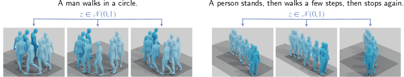
Figure 1: Goal: Text-to-Motions (TEMOS) learns to synthesize human motion sequences conditioned on a textual description and a duration. SMPL pose sequences are generated by sampling from a single latent vector, $z$. Here, we illustrate the diversity of our motions on two sample texts, providing three generations per text input. Each image corresponds to a motion sequence where we visualize the root trajectory projected on the ground plane and the human poses at multiple equidistant time frames. The flow of time is shown with a color code where lighter blue denotes the past.

Despite recent efforts in this area, most current methods generate only one output motion per text input [30, 2, 14]. That is, with the input “A man walks in a circle”, these methods synthesize one motion. However, one description often can map to multiple ways of performing the actions, often due to ambiguities and lack of details, e.g., in our example, the size and the orientation of the circle are not specified. An ideal generative model should therefore be able to synthesize multiple sequences that respect the textual description while exploring the degrees of freedom to generate natural variations. While, in theory, the more precise the description becomes, the less space there is for diversity; it is a desirable property for natural language interfaces to manage intrinsic ambiguities of linguistic expressions [13]. In this paper, we propose a method that allows sampling from a distribution of human motions conditioned on natural language descriptions. Figure 1 illustrates multiple sampled motions generated from two input texts; check the project webpage [41] for video examples.

A key challenge is building models that are effective for temporal modeling. Most prior work employs autoregressive models that iteratively decode the next time frame given the past. These approaches may suffer from drift over time and often, eventually, produce static poses [37]. In contrast, sequence-level generative models encode an entire sequence and can exploit long-range context. In this work, we incorporate the powerful Transformer models [52], which have proven effective for various sequence modeling tasks [9, 4]. We design a simple yet effective architecture, where both the motion and text are input to Transformer encoders before projecting them to a cross-modal joint space. Similarly, the motion decoder uses a Transformer architecture taking positional encodings and a latent vector as input, and generating a 3D human motion (see Figure 2). Notably, a single sequence-level latent vector is used to decode the motion in one shot, without any autoregressive iterations. Through detailed ablation studies, we show that the main improvement over prior work stems from this design.

A well-known challenge common to generative models is the difficulty of evaluation. While many metrics are used in evaluating generated motions, each of them is limited. Consequently, in this work, we rely on both quantitative measures that compare against the ground truth motion data associated with each test description, and human perceptual studies to evaluate the perceived quality of the motions. The former is problematic particularly for this work, because it assumes one true motion per text, but our method produces multiple motions due to its probabilistic nature. We find that human judgment of motion quality is necessary for a full picture.

Moreover, the state of the art reports results on the task of future motion prediction. Specifically, Ghosh et al. [14] assume the first pose in the generated sequence is available from the ground truth. In contrast, we evaluate our method by synthesizing the full motion from scratch; i.e. without conditioning on the first, ground truth, frame. We provide results for various settings, e.g., comparing a random generation against the ground truth, or picking the best out of several generations. We outperform previous work even when sampling a single random generation, but the performance improves as we increase the number of generations and pick the best.

A further addition we make over existing text-to-motion approaches is to generate sequences of SMPL body models [33]. Unlike classical skeleton representations, the parametric SMPL model provides the body surface, which can support future research on motions that involve interaction with objects or the scene. Such skinned generations were considered in other work on unconstrained or action-conditioned generation [63, 42]. Here, we demonstrate promising results for the text-conditioning scenario as well. The fact that the framework supports multiple body representations, illustrates its generality.

In summary, our contributions are the following: (i) We present Text-to-Motions (TEMOS), a novel cross-modal variational model that can produce diverse 3D human movements given textual descriptions in natural language. (ii) In our experiments, we provide an extensive ablation study of the model components and outperform the state of the art by a large margin both on standard metrics and through perceptual studies. (iii) We go beyond stick figure generations, and exploit the SMPL model for text-conditioned body surface synthesis, demonstrating qualitatively appealing results. The code and trained models are available on our project page [41].

2 Related work

We provide a brief summary of relevant work on human motion synthesis and text-conditioned motion generation. While there is also work on facial motion generation [24, 8, 46, 12], here we focus on articulated human bodies.

Human motion synthesis. While there is a large body of work focusing on future human motion prediction [40, 17, 6, 3, 63, 60] and completion [10, 18], here, we give an overview of methods that generate motions from scratch (i.e., no past or future observations). Generative models of human motion have been designed using GANs [1, 31], VAEs [16, 42], or normalizing flows [19, 61]. In this work, we employ VAEs in the context of Transformer neural network architectures. Recent work suggest that VAEs are effective for human motion generation compared with GANs [16, 42], while being easier to train.

Motion synthesis methods can be broadly divided into two categories: (i) unconstrained generation, which models the entire space of possible motions [57, 64, 62] and (ii) conditioned synthesis, which aims for controllability such as using music [27, 28, 29], speech [7, 15], action [16, 42], and text [30, 31, 1, 2, 14, 49] conditioning. Generative models that synthesize unconstrained motions aim, by design, to sample from a distribution, allowing generation of diverse motions. However, they lack the ability to control the generation process. On the other hand, the conditioned synthesis can be further divided into two categories: deterministic [30, 2, 14] or probabilistic [1, 31, 27, 28, 16, 42]. In this work, we focus on the latter, motivated by the fact that there are often multiple possible motions for a given condition.

Text-conditioned motion generation. Recent work explores the advances in natural language modeling [38, 9] to design sequence-to-sequence approaches to cast the text-to-motion task as a machine translation problem [44, 30, 1]. Others build joint cross-modal embeddings to map the text and motion to the same space [56, 2, 14], which has been a success in other research area [45, 59, 58, 5].

Several methods use an impoverished body motion representation. For example, some do not model the global trajectory [44, 56], making the motions unrealistic and ignoring the global movement description in the input text. Text2Action [1] uses a sequence-to-sequence model but only models the upper body motion. This is because Text2Action uses a semi-automatic approach to create training data from the MSR-VTT captioned video dataset [54], which contains frequently occluded lower bodies. They apply 2D pose estimation, lift the joints to 3D, and employ manual cleaning of the input text to make it generic.

Most other work uses 3D motion capture data [30, 31, 2, 14]. DVGANs [31] adapt the CMU MoCap database [51] and Human3.6M [22, 23] for the task of motion generation and completion, and they use the action labels as text-conditioning instead of categorical supervision. More recent works [30, 2, 14] employ the KIT Motion-Language dataset [43], which is also the focus of our work.

A key limitation of many state-of-the-art text-conditioned motion generation models is that they are deterministic [2, 14]. These methods employ a shared cross-modal latent space approach. Ahuja et al. [2] employ word2vec text embeddings [38], while [14] uses the more recent BERT model [9].

Most similar to our work is Ghosh et. al. [14], which builds on Language2Pose [2]. Our key difference is the integration of a variational approach for sampling a diverse set of motions from a single text. Our further improvements include the use of Transformers to encode motion sequences into a single embedding instead of the autoregressive approach in [14]. This allows us to encode distribution parameters of the VAE as in [42], proving effective in our state-of-the-art results. Ghosh et al. [14] also encode the upper body and lower body separately, whereas our approach does not need such hand crafting.

3 Generating multiple motions from a textual description

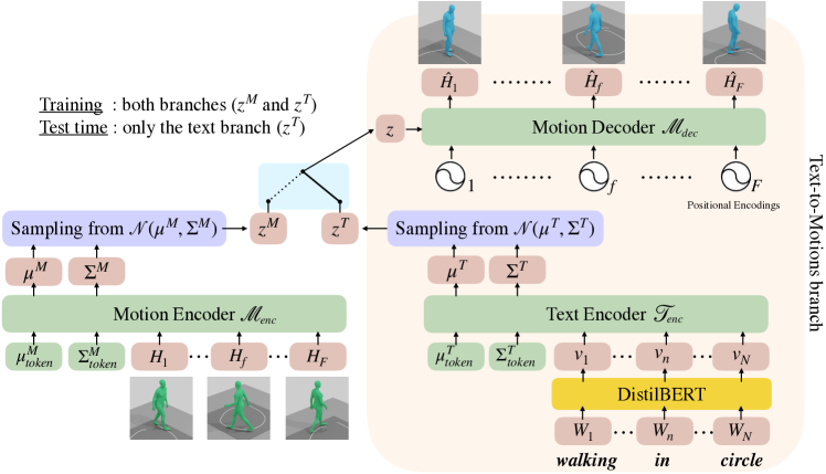
Figure 2: Method overview: During training, we encode both the motion and text through their respective Transformer encoders, together with modal-specific learnable distribution tokens. The encoder outputs corresponding to these tokens provide Gaussian distribution parameters on which the KL losses are applied and a latent vector $z$ is sampled. Reconstruction losses on the motion decoder outputs further provide supervision for both motion and text branches. In practice, our word embedding consists of a variational encoder that takes input from a pre-trained and frozen DistilBERT [48] model. Trainable layers are denoted in green, the inputs/outputs in brown. At test time, we only use the right branch, which goes from an input text to a diverse set of motions through the random sampling of the latent vector $z^{T}$ on the cross-modal space. The output motion duration is determined by the number of positional encodings $F$.

In this section, we start by formulating the problem (Section 3.1). We then provide details on our model design (Section 3.2), as well as our training strategy (Section 3.3).

3.1 Task definition

Given a sentence describing a motion, the goal is to generate various sequences of 3D human poses and trajectories that match the textual input. Next, we describe the representation for the text and motion data.

Textual description represents a written natural language sentence (e.g., in English) that describes what and how a human motion is performed. The sentence can include various levels of detail: a precise sequence of actions such as “A human walks two steps and then stops” or a more ambiguous description such as “A man walks in a circle”. The data structure is a sequence of words $W_{1:N}=W_{1},\ldots,W_{N}$ from the English vocabulary.

3D human motion is defined as a sequence of human poses $H_{1:F}=H_{1},\ldots,H_{F}$, where $F$ denotes the number of time frames. Each pose $H_{f}$ corresponds to a representation of the articulated human body. In this work, we employ two types of body motion representations: one based on skeletons, one based on SMPL [33]. First, to enable a comparison with the state of the art, we follow the rotation-invariant skeleton representation from Holden et. al. [21], which is used in the previous work we compare with [2, 14]. Second, we incorporate the parametric SMPL representation by encoding the global root trajectory of the body and parent-relative joint rotations in 6D representation [65]. We provide detailed formulations for both motion representations in Appendix 0.B.

More generally, a human motion can be represented by a sequence of $F$ poses each with $p$ dimensions, so that at frame $f$, we have $H_{f}\in\mathbb{R}^{p}$. Our goal is, given a textual description $W_{1:N}$, to sample from a distribution of plausible motions $H_{1:F}$ and to generate multiple hypotheses.

3.2 TEMOS model architecture

Following [2], we learn a joint latent space between the two modalities: motion and text (see Figure 2). To incorporate generative modeling in such an approach, we employ a VAE [26] formulation that requires architectural changes. We further employ Transformers [52] to obtain sequence-level embeddings both for the text and motion data. Next, we describe the two encoders for motion and text, followed by the motion decoder.

Motion and text encoders. We have two encoders for representing motion $\mathscr{M}_{enc}$ and text $\mathscr{T}_{enc}$ in a joint space. The encoders are designed to be as symmetric as possible across the two modalities. To this end, we adapt the ACTOR [42] Transformer-based VAE motion encoder by making it class-agnostic (i.e., removing action conditioning). This encoder takes as input a sequence of vectors of arbitrary length, as well as learnable distribution tokens. The outputs corresponding to the distribution tokens are treated as Gaussian distribution parameters $\mu$ and $\Sigma$ of the sequence-level latent space. Using the reparameterization trick [26], we sample a latent vector $z\in\mathbb{R}^{d}$ from this distribution (see Figure 2). The latent space dimensionality $d$ is set to 256 in our experiments.

For the motion encoder $\mathscr{M}_{enc}$, the input sequence of vectors is $H_{1:F}$, representing the poses. For the text encoder $\mathscr{T}_{enc}$, the inputs are word embeddings for $W_{1:N}$ obtained from a pretrained language model DistilBERT [48]. We freeze the weights of DistilBERT unless stated otherwise.

Motion decoder. The motion decoder $\mathscr{M}_{dec}$ is a Transformer decoder (as in ACTOR [42], but without the bias token to make it class agnostic), so that given a latent vector $z$ and a duration $F$, we generate a 3D human motion sequence $\widehat{H}_{1:F}$ non-autoregressively from a single latent vector. Note that such approach does not require masks in self-attention, and tends to provide a globally consistent motion. The latent vector is obtained from one of the two encoders during training (described next, in Section 3.3), and the duration is represented as a sequence of positional encodings in the form of sinusoidal functions. We note that our model can produce variable durations, which is another source of diversity (see supplementary video [41]).

3.3 Training strategy

For our cross-modal neural network training, we sample a batch of text-motion pairs at each training iteration. In summary, both input modalities go through their respective encoders, and both encoded vectors go through the motion decoder to reconstruct the 3D poses. This means we have one branch that is text-to-motion and another branch that is an autoencoder for motion-to-motion (see Figure 2). At test time, we only use the text-to-motion branch. This approach proved effective in previous work [2]. Here, we first briefly describe the loss terms to train this model probabilistically. Then, we provide implementation details.

Given a ground-truth pair consisting of human motion $H_{1:F}$ and textual description $W_{1:N}$, we use (i) two reconstruction losses – one per modality, (ii) KL divergence losses comparing each modality against Gaussion priors, (iii) KL divergence losses, as well as a cross-modal embedding similarity loss to compare the two modalities to each other.

Reconstruction losses ($\mathcal{L}_{\text{R}}$). We obtain $\widehat{H}^{M}_{1:F}$ and $\widehat{H}^{T}_{1:F}$ by inputting the motion embedding and text embedding to the decoder, respectively. We compare these motion reconstructions to the ground-truth human motion $H_{1:F}$ via:

$$\mathcal{L}_{\text{R}}=\mathscr{L}_{1}(H_{1:F},\widehat{H}^{M}_{1:F})+\mathscr{L}_{1}(H_{1:F},\widehat{H}^{T}_{1:F})$$ (1)

where $\mathscr{L}_{1}$ denotes the smooth L1 loss.

KL losses ($\mathcal{L}_{\text{KL}}$). To enforce the two modalities to be close to each other in the latent space, we minimize the Kullback-Leibler (KL) divergences between the distributions of the text embedding $\phi^{T}=\mathcal{N}(\mu^{T},\Sigma^{T})$ and the motion embedding $\phi^{M}=\mathcal{N}(\mu^{M},\Sigma^{M})$. To regularize the shared latent space, we encourage each distribution to be similar to a normal distribution $\psi=\mathcal{N}(0,I)$ (as in standard VAE formulations). Thus we obtain four terms:

$$\begin{split}\mathcal{L}_{\text{KL}}&=\text{KL}(\phi^{T},\phi^{M})+\text{KL}(\phi^{M},\phi^{T})\\ &+\text{KL}(\phi^{T},\psi)+\text{KL}(\phi^{M},\psi).\end{split}$$ (2)

Cross-modal embedding similarity loss ($\mathcal{L}_{\text{E}}$). After sampling the text embedding $z^{T}\sim\mathcal{N}(\mu^{T},\Sigma^{T})$ and the motion embedding $z^{M}\sim\mathcal{N}(\mu^{M},\Sigma^{M})$ from the two encoders, we also constrain them to be as close as possible to each other, with the following loss term (i.e., loss between the cross-modal embeddings):

$$\begin{split}\mathcal{L}_{\text{E}}&=\mathscr{L}_{1}(z^{T},z^{M}).\end{split}$$ (3)

The resulting total loss is defined as a weighted sum of the three terms: $\mathcal{L}=\mathcal{L}_{\text{R}}+\lambda_{\text{KL}}\mathcal{L}_{\text{KL}}+\lambda_{\text{E}}\mathcal{L}_{\text{E}}$. We empirically set $\lambda_{\text{KL}}$ and $\lambda_{\text{E}}$ to $10^{-5}$, and provide ablations. While some of the loss terms may appear redundant, we experimentally validate each term.

Implementation details. We train our models for 1000 epochs with the AdamW optimizer [25, 34] using a fixed learning rate of $10^{-4}$. Our minibatch size is set to 32. Our Transformer encoders and decoders consist of 6 layers for both motion and text encoders, as well the motion decoder. Ablations about these hyperparameters are presented in Appendix 0.A.

At training time, we input the full motion sequence, i.e., a variable number of frames for each training sample. At inference time, we can specify the desired duration $F$ (see supplementary video [41]); however, we provide quantitative metrics with known ground-truth motion duration.

4 Experiments

We first present the data and performance measures used in our experiments (Section 4.1). Next, we compare to previous work (Section 4.2) and present an ablation study (Section 4.3). Then, we demonstrate our results with the SMPL model (Section 4.4). Finally, we discuss limitations (Section 4.5).

4.1 Data and evaluation metrics

KIT Motion-Language [43] dataset (KIT) provides raw motion capture (MoCap) data, as well as processed data using the Master Motor Map (MMM) framework [50]. The motions comprise a collection of subsets of the KIT Whole-Body Human Motion Database [36] and of the CMU Graphics Lab Motion Capture Database [51]. The dataset consists of 3911 motion sequences with 6353 sequence-level description annotations, with 9.5 words per description on average. We use the same splits as in Language2Pose [2] by extracting 1784 training, 566 validation and 587 test motions (some motions do not have corresponding descriptions). As the model from Ghosh et al. [14] produce only 520 sequences in the test set (instead of 587), for a fair comparison we evaluate all methods with this subset, which we will refer to as the test set. If the same motion sequence corresponds to multiple descriptions, we randomly choose one of these descriptions at each training iteration, while we evaluate the method on the first description. Recent state-of-the-art methods on text-conditioned motion synthesis employ this dataset, by first converting the MMM axis-angle data into 21 $xyz$ coordinates and downsampling the sequences from 100 Hz to 12.5 Hz. We do the same procedure, and follow the training and test splits explained above to compare methods. Additionally, we find correspondences from the KIT sequences to the AMASS MoCap collection [35] to obtain the motions in SMPL body format. We note that this procedure resulted in a subset of 2888 annotated motion sequences, as some sequences have not been processed in AMASS. We refer to this data as KIT${}_{\text{SMPL}}$.

Evaluation metrics. We follow the performance measures employed in Language2Pose [2] and Ghosh et al. [14] for quantitative evaluations. In particular, we report Average Positional Error (APE) and Average Variance Error (AVE) metrics. However, we note that the results in [14] do not match the ones in [2] due to lack of evaluation code from [2]. We identified minor issues with the evaluation code of [14] (more details in Appendix 0.C); therefore, we reimplement our own evaluation. Moreover, we introduce several modifications (which we believe make the metrics more interpretable): in contrast to [14, 2], we compute the root joint metric by using the joint coordinates only (and not on velocities for $x$ and $y$ axes) and all the metrics are computed without standardizing the data (i.e., mean subtraction and division by standard deviation). Our motivation for this is to remain in the coordinate space since the metrics are positional. Note that the KIT data in the MMM format is canonicalized to the same body shape. We perform most of our experiments with this data format to remain comparable to the state of the art. We report results with the SMPL body format separately since the skeletons are not perfectly compatible (see Appendix 0.A.6). Finally, we convert our low-fps generations (at 12 Hz) to the original frame-rate of KIT (100 Hz) via linear interpolation on coordinates and report the error comparing to this original ground truth. We display the error in meters.

As discussed in Section 1, the evaluation is suboptimal because it assumes one ground truth motion per text; however, our focus is to generate multiple different motions. The KIT test set is insufficient to design distribution-based metrics such as FID, since there are not enough motions for the same text (see Appendix 0.E for statistics). We therefore report the performance of generating a single sample, as well as generating multiple and evaluating the closest sample to the ground truth. We rely on additional perceptual studies to assess the correctness of multiple generations, which is described in Appendix 0.C.

4.2 Comparison to the state of the art

Quantitative. We compare with the state-of-the-art text-conditioned motion generation methods [30, 2, 14] on the test set of the KIT dataset (as defined in 4.1). To obtain motions for these three methods, we use their publicly available codes (note that all three give the ground truth initial frame as input to their generations). We summarize the main results in Table 1. Our TEMOS approach substantially outperforms on all metrics, except APE on local joints. As pointed by [2, 14], the most difficult metric that better differentiates improvements on this dataset is the APE on the root joint, and we obtain significant improvements on this metric. Moreover, we sample a random latent vector for reporting the results for TEMOS; however, as we will show next in Section 4.3, if we sample more, we are more likely to find the motion closer to the ground truth.

Qualitative. We further provide qualitative comparisons in Figure 4 with the state of the art. We show sample generations for Lin et al. [30], JL2P [2], and Ghosh et al. [14]. The motions from our TEMOS model reflect the semantic content of the input text better than the others across a variety of samples. Furthermore, we observe that while [30] generates overly smooth motions, JL2P has lots of foot sliding. [14], on the other hand, synthesizes unrealistic motions due to exaggerated foot contacts (and even extremely elongated limbs such as in 3rd column, 3rd row of Figure 4). Our generations are the most realistic among all. Further visualizations are provided in the supplementary video [41].

Perceptual study. These conclusions are further justified by two human perceptual studies that evaluate which methods are preferred in terms of semantics (correspondence to the text) or in terms of realism. For the first study, we displayed a pair of motions (with a randomly swapped order in each display) and a description of the motion, and asked Amazon Mechanical Turk (AMT) workers the question: “Which motion corresponds better to the textual description?”. We collected answers for 100 randomly sampled test descriptions, showing each description to multiple workers. For the second study, we asked another set of AMT workers the question: “Which motion is more realistic?” without showing the description. We give more details on our perceptual studies in Appendix 0.C.

Table 1: State-of-the-art comparison: We compare our method with recent works [30, 2, 14], on the KIT Motion-Language dataset [43] and obtain significant improvements on most metrics (values in meters) even if we are sampling a random motion per text conditioning for our model.

Methods	Average Positional Error $\downarrow$				Average Variance Error $\downarrow$
	root joint	global traj.	mean local	mean global	root joint	global traj.	mean local	mean global
Lin et. al. [30]	1.966	1.956	0.105	1.969	0.790	0.789	0.007	0.791
JL2P [2]	1.622	1.616	0.097	1.630	0.669	0.669	0.006	0.672
Ghosh et al. [14]	1.291	1.242	0.206	1.294	0.564	0.548	0.024	0.563
TEMOS (ours)	0.963	0.955	0.104	0.976	0.445	0.445	0.005	0.448

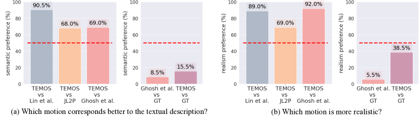
Figure 3: Perceptual study: (a) We ask users which motion corresponds better to the input text between two displayed samples generated from model A vs model B. (b) We ask other users which motion is more realistic without showing the textual description. We report the percentage for which the users show a preference for A. The red dashed line denotes the 50% level (equal preference). On the left of both studies, our generations from TEMOS were rated better than the previous work of Lin et al. [30], JL2P [2], and Ghosh et al. [14]. On the right of both studies, we compare against the ground truth (GT) and see that our motions are rated as better than the GT 15.5% and 38.5% of the time, whereas Ghosh et al. [14] are at 8.5% and 5.5%.

The resulting ranking between our method and each of the state-of-the-art methods [30, 2, 14] is reported in Figure 3. We see that humans perceive our motions as better matching the descriptions compared to all three state-of-the-art methods, especially significantly outperforming Lin et al. [30] (users preferred TEMOS over [30] 90.5% of the time). For the more competitive and more recent Ghosh et al. [14] method, we ask users to compare their generations against the ground truth. We do the same for our generations and see that users preferred our motions over the ground truth 15.5% of the time where the ones from Ghosh et al. [14] are preferred only 8.5% of the time. Our generations are also clearly preferred in terms of realism over the three methods. Our motions are realistic enough that they are preferred to real motion capture data 38.5% of the time, as compared to 5.5% of the time for Ghosh et al. [14].

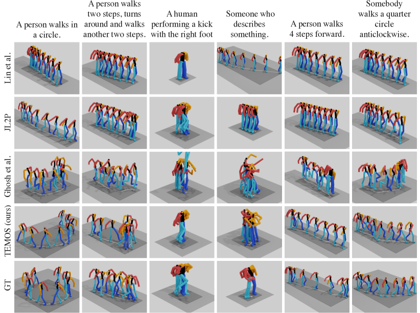
Figure 4: Qualitative comparison to the state of the art: We qualitatively compare the generations from our TEMOS model with the recent state-of-the-art methods and the ground truth (GT). We present different textual queries in columns, and different methods in rows. Overall, our generations better match semantically to the textual descriptions. We further overcome several limitations with the prior work, such as over-smooth motions in Lin et al. [30], foot sliding in J2LP [2], and exaggerated foot contacts in Ghosh et al. [14], which can better be viewed in our supplementary video [41].

Table 2: Variational vs deterministic models: We first provide the performance of the deterministic version of our model. We then report results with several settings using our variational model: (i) generating a single motion per text to compare against the ground truth (either randomly or using a zero-vector representing the mean of the Gaussian latent space), and (ii) generating 10 motions per text, each compared against the ground truth separately (either averaging the metrics or taking the motion with the best metric). As expected, TEMOS is able to produce multiple hypotheses where the best candidates improve the metrics.

Model	Sampling	Average Positional Error $\downarrow$				Average Variance Error $\downarrow$
		root joint	global traj.	mean local	mean global	root joint	global traj.	mean local	mean global
Deterministic	n/a	1.175	1.165	0.106	1.188	0.514	0.513	0.005	0.516
Variational	1 sample, $z=\vec{0}$	1.005	0.997	0.104	1.020	0.443	0.442	0.005	0.446
Variational	1 random sample	0.963	0.955	0.104	0.976	0.445	0.445	0.005	0.448
Variational	10 random avg	1.001	0.993	0.104	1.015	0.451	0.451	0.005	0.454
Variational	10 random best	0.784	0.774	0.104	0.802	0.392	0.391	0.005	0.395

4.3 Ablation study

In this section, we evaluate the influence of several components of our framework in a controlled setting.

Variational design. First, we ‘turn off’ the variational property of our generative model and synthesize a single motion per text. Instead of two learnable distribution tokens as in Figure 2, we use one learnable embedding token from which we directly obtain the latent vector using the corresponding encoder output (hence removing sampling). We removed all the KL losses such that the model becomes deterministic, and keep the embedding similarity loss to learn the joint latent space. In Table 2, we report performance metrics with this approach and see that we already obtain competitive performance with the deterministic version of our model, demonstrating the improvements from our temporal sequence modeling approach compared to previous works.

As noted earlier, our variational model can produce multiple generations for the same text, and a single random sample may not necessarily match the ground truth. In Table 2, we report results for one generation from a random $z$ noise vector, or generating from the zero-vector that represents the mean of the latent space ($z=\vec{0}$); both perform similarly. To assess the performance with multiple generations, we randomly sample 10 latent vectors per text, and provide two evaluations. First, we compare each of the 10 generations to the single ground truth, and average over all generations (10 random avg). Second, we record the performance of the motion that best matches to the ground truth out of the 10 generations (10 random best). As expected, Table 2 shows improvements with the latter (see Appendix 0.A.5 for more values for the number of latent vectors).

Architectural and loss components. Next, we investigate which component is most responsible for the performance improvement over the state of the art, since even the deterministic variant of our model outperforms previous works. Table 3 reports the performance by removing one component at each row. The APE root joint performance drops from 0.96 to i) 1.44 using GRUs instead of Transformers; ii) 1.18 without the motion encoder (using only one KL loss); iii) 1.09 without the cross-modal embedding loss; iv) 1.05 without the Gaussian priors; v) 0.99 without the cross-modal KL losses. Note that the cross-modal framework originates from JL2P [2]. While we observe slight improvement with each of the cross-modal terms, we notice that the model performance is already satisfactory even without the motion encoder. We therefore conclude that the main improvement stems from the improved non-autoregressive Transformer architecture, and removing each of the other components (4 KL loss terms, motion encoder, embedding similarity) also slightly degrades performance.

Table 3: Architectural and loss study: We conclude that the most critical component is the Transformer architecture, as opposed to a recurrent one (i.e., GRU). While the additional losses are helpful, they bring relatively minor improvements.

			Average Positional Error $\downarrow$				Average Variance Error $\downarrow$
			root	glob.	mean	mean	root	glob.	mean	mean
Arch.	$\mathcal{L}_{KL}$	$\mathcal{L}_{E}$	joint	traj.	loc.	glob.	joint	traj.	loc.	glob.
GRU	$KL(\phi^{T},\phi^{M})+KL(\phi^{M},\phi^{T})+KL(\phi^{T},\psi)+KL(\phi^{M},\psi)$	✓	1.443	1.433	0.105	1.451	0.600	0.599	0.007	0.601
Transf.	$KL(\phi^{T},\psi)$ w/out $\mathscr{M}_{enc}$	✗	1.178	1.168	0.106	1.189	0.506	0.505	0.006	0.508
Transf.	$KL(\phi^{T},\phi^{M})+KL(\phi^{M},\phi^{T})+KL(\phi^{T},\psi)+KL(\phi^{M},\psi)$	✗	1.091	1.083	0.107	1.104	0.449	0.448	0.005	0.451
Transf.	$KL(\phi^{T},\psi)+KL(\phi^{M},\psi)$ w/out cross-modal KL losses	✗	1.080	1.071	0.107	1.095	0.453	0.452	0.005	0.456
Transf.	$KL(\phi^{T},\psi)+KL(\phi^{M},\psi)$ w/out cross-modal KL losses	✓	0.993	0.983	0.105	1.006	0.461	0.460	0.005	0.463
Transf.	$KL(\phi^{T},\phi^{M})+KL(\phi^{M},\phi^{T})$ w/out Gaussian priors	✓	1.049	1.039	0.108	1.065	0.472	0.471	0.005	0.475
Transf.	$KL(\phi^{T},\phi^{M})+KL(\phi^{M},\phi^{T})+KL(\phi^{T},\psi)+KL(\phi^{M},\psi)$	✓	0.963	0.955	0.104	0.976	0.445	0.445	0.005	0.448

Language model finetuning. As explained in Section 3.2, we do not update the language model parameters during training, which are from the pretrained DistilBERT [48]. We measure the performance with and without finetuning in Table 4 and conclude that freezing performs better while being more efficient. We note that we already introduce additional layers through our text encoder (see Figure 2), which may be sufficient to adapt the embeddings to our specific motion description domain. We provide an additional experiment with larger language models in Appendix 0.A.4.

Table 4: Language model finetuning: We experiment with finetuning the language model (LM) parameters (i.e., DistilBERT [48]) end-to-end with our motion-language cross-modal framework, and do not observe improvements. Here ‘Frozen’ refers to not updating the LM parameters.

LM params	Average Positional Error $\downarrow$				Average Variance Error $\downarrow$
	root joint	global traj.	mean local	mean global	root joint	global traj.	mean local	mean global
Finetuned	1.402	1.393	0.113	1.414	0.559	0.558	0.006	0.562
Frozen	0.963	0.955	0.104	0.976	0.445	0.445	0.005	0.448

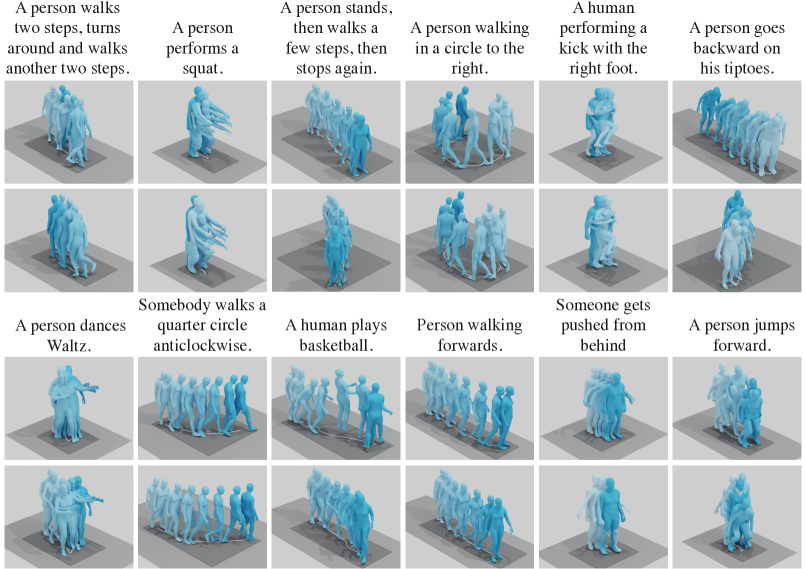
Figure 5: Qualitative evaluation of the diversity: We display two motion generations for each description. Our model shows certain diversity among different generations while respecting the textual description.

4.4 Generating skinned motions

We evaluate the variant of our model which uses the parametric SMPL representation to generate full body meshes. The quantitative performance metrics on KIT${}_{\text{SMPL}}$ test set can be found in Appendix 0.A.6. We provide qualitative examples in Figure 5 to illustrate the diversity of our generations for a given text. For each text, we present 2 random samples. Each column shows a different text input. For all the visualization renderings in this paper, the camera is fixed and the bodies are sampled evenly across time. Moreover, the forward direction of the first frame is always facing the same canonical direction. Our observation is that the model can generate multiple plausible motions corresponding to the same text, exploring the degrees of freedom remaining from ambiguities in the language description. On the other hand, if the text describes a precise action, such as ‘A person performs a squat’ the diversity is reduced. The results are better seen as movies; see supplementary video [41], where we also display other effects such as generating variable durations, and interpolating in the latent space.

4.5 Limitations

Our model has several limitations. Firstly, the vocabulary of the KIT data is relatively small with 1263 unique words compared to the full open-vocabulary setting of natural language, and are dominated by locomotive motions. We therefore expect our model to suffer from out-of-distribution descriptions. Moreover, we do not have a principled way of measuring the diversity of our models since the training does not include multiple motions for the exact same text. Secondly, we notice that if the input text contains typos (e.g., ‘wals’ instead of ‘walks’), TEMOS might drastically fail, suggesting that a preprocessing step to correct them beforehand might be needed. Finally, our method cannot scale up to very long motions (such as walking for several minutes) due to the quadratic memory cost.

5 Conclusion

In this work, we introduced a variational approach to generate diverse 3D human motions given textual descriptions in the form of natural language. In contrast to previous methods, our approach considers the intrinsically ambiguous nature of language and generates multiple plausible motions respecting the textual description, rather than deterministically producing only one. We obtain state-of-the-art results on the widely used KIT Motion-Language benchmark, outperforming prior work by a large margin both in quantitative experiments and perceptual studies. Our improvements are mainly from the architecture design of incorporating sequence modeling via Transformers. Furthermore, we employ full body meshes instead of only skeletons. Future work should focus on explicit modeling of contacts and integrating physics knowledge. Another interesting direction is to explore duration estimation for the generated motions. While we do not expect any immediate negative societal impact from our work, we note that with the potential advancement of fake visual data generation, a risk may arise from the integration of our model in the applications that animate existing people without their consent, raising privacy concerns.

Acknowledgements. This work was granted access to the HPC resources of IDRIS under the allocation 2021-AD011012129R1 made by GENCI. GV acknowledges the ANR project CorVis ANR-21-CE23-0003-01, and research gifts from Google and Adobe. The authors would like to thank Monika Wysoczanska, Georgy Ponimatkin, Romain Loiseau, Lucas Ventura and Margaux Lasselin for their feedbacks, Tsvetelina Alexiadis and Taylor McConnell for helping with the perceptual study, and Anindita Ghosh for helping with the evaluation details on the KIT dataset.

Disclosure: https://files.is.tue.mpg.de/black/CoI_ECCV_2022.txt

APPENDIX

This appendix provides additional experiments (Section 0.A), description of the motion representations (Section 0.B), details on evaluation metrics (Section 0.C), implementation details (Section 0.D), and dataset statistics (Section 0.E).

0..0.1 Video.

Additionally, we provide a supplemental video, available on our website [41], which we encourage the reader to watch since motion is critical in our results, and this is hard to convey in a static document. In the video, we illustrate: (i) comparison with previous work, (ii) training with skeleton versus SMPL data, (iii) diversity of our model, (iv) generation of variable size sequences, (v) interpolation between two texts in our latent space, and (vi) failure cases.

0..0.2 Code.

We also share our code base on the project page [41], which reproduces our training and evaluation metrics. Explanations on how to configure the data and launch the training can be found in the file README.md.

Appendix 0.A Additional experiments

We conduct several experiments to explore the sensitivity of our model to certain hyperparameters. Our final set of hyperparameters was chosen using the validation set (starting from a set of hyperparameters similar to ACTOR [42]). Note that these hyperparameters did not always appear optimal on the test set. The following ablations provide a sense of robustness to different parameters. In particular, we show the effects of the batch size (Section 0.A.1), $\{\lambda_{\text{KL}},\lambda_{\text{E}}\}$ loss weighting parameters (Section 0.A.2) and the architecture parameters of Transformers (Section 0.A.3). All other parameters, such as the learning rate ($10^{-4}$), the optimizer (AdamW) and the number of epochs ($1000$) are fixed. For all these experiments we use the skeleton-based MMM representation.

We also experiment with various pretrained language models (Section 0.A.4).

Note that the evaluation is based on a single random sample. All results can be improved by taking the best sample closest to the ground truth out of multiple generations (as next explained in Section 0.A.5). We also experiment with taking the sample farthest from the ground truth.

Finally, in Section 0.A.6, we report quantitative results for our model trained with SMPL rotations.

0.A.1 Batch size

Table A.1: Batch size: We see that the performance is the best for either a small batch size (=8) or a bigger batch size (=32). We were unable to use a higher batch size due to the GPU memory limit.

Batch size	Average Positional Error $\downarrow$				Average Variance Error $\downarrow$
	root joint	global traj.	mean local	mean global	root joint	global traj.	mean local	mean global
bs = 8	0.950	0.941	0.105	0.965	0.449	0.448	0.005	0.451
bs = 16	1.115	1.106	0.105	1.128	0.513	0.512	0.005	0.515
bs = 24	1.260	1.250	0.106	1.273	0.542	0.542	0.005	0.545
bs = 32	0.963	0.955	0.104	0.976	0.445	0.445	0.005	0.448

Table A.2: Weight of the KL losses ($\lambda_{\text{KL}}$) and the embedding loss ($\lambda_{\text{E}}$): The results are influenced more by changes in $\lambda_{\text{E}}$ than in $\lambda_{\text{KL}}$, but otherwise if the values are not too low, the performances are similar. Note that the control row $\lambda_{\text{KL}}=10^{-5},\lambda_{\text{E}}=10^{-5}$ is repeated in each block.

Losses weight	Average Positional Error $\downarrow$				Average Variance Error $\downarrow$
	root joint	global traj.	mean local	mean global	root joint	global traj.	mean local	mean global
$\lambda_{\text{KL}}=\lambda_{\text{E}}=10^{-3}$	1.219	1.210	0.111	1.230	0.555	0.554	0.006	0.556
$\lambda_{\text{KL}}=\lambda_{\text{E}}=10^{-4}$	1.110	1.101	0.106	1.122	0.476	0.475	0.005	0.479
$\lambda_{\text{KL}}=\lambda_{\text{E}}=10^{-5}$	0.963	0.955	0.104	0.976	0.445	0.445	0.005	0.448
$\lambda_{\text{KL}}=\lambda_{\text{E}}=10^{-6}$	1.242	1.233	0.105	1.254	0.586	0.585	0.005	0.589
$\lambda_{\text{KL}}=\lambda_{\text{E}}=10^{-7}$	1.034	1.025	0.108	1.049	0.488	0.487	0.005	0.491
$\lambda_{\text{KL}}=\lambda_{\text{E}}=10^{-8}$	1.085	1.075	0.107	1.099	0.490	0.489	0.005	0.493
$\lambda_{\text{KL}}=10^{-5},\lambda_{\text{E}}=10^{-3}$	1.293	1.284	0.107	1.305	0.631	0.631	0.005	0.635
$\lambda_{\text{KL}}=10^{-5},\lambda_{\text{E}}=10^{-4}$	1.039	1.029	0.104	1.052	0.449	0.448	0.005	0.452
$\lambda_{\text{KL}}=10^{-5},\lambda_{\text{E}}=10^{-5}$	0.963	0.955	0.104	0.976	0.445	0.445	0.005	0.448
$\lambda_{\text{KL}}=10^{-5},\lambda_{\text{E}}=10^{-6}$	1.082	1.072	0.107	1.095	0.456	0.455	0.005	0.459
$\lambda_{\text{KL}}=10^{-5},\lambda_{\text{E}}=10^{-7}$	1.018	1.008	0.106	1.031	0.464	0.463	0.005	0.467
$\lambda_{\text{KL}}=10^{-5},\lambda_{\text{E}}=10^{-8}$	1.076	1.067	0.105	1.089	0.477	0.476	0.005	0.480
$\lambda_{\text{KL}}=10^{-3},\lambda_{\text{E}}=10^{-5}$	1.145	1.135	0.111	1.157	0.507	0.506	0.006	0.509
$\lambda_{\text{KL}}=10^{-4},\lambda_{\text{E}}=10^{-5}$	1.070	1.061	0.106	1.083	0.471	0.470	0.005	0.474
$\lambda_{\text{KL}}=10^{-5},\lambda_{\text{E}}=10^{-5}$	0.963	0.955	0.104	0.976	0.445	0.445	0.005	0.448
$\lambda_{\text{KL}}=10^{-6},\lambda_{\text{E}}=10^{-5}$	0.971	0.962	0.105	0.986	0.455	0.454	0.005	0.457
$\lambda_{\text{KL}}=10^{-7},\lambda_{\text{E}}=10^{-5}$	1.140	1.132	0.106	1.154	0.513	0.512	0.005	0.517
$\lambda_{\text{KL}}=10^{-8},\lambda_{\text{E}}=10^{-5}$	1.025	1.015	0.107	1.039	0.461	0.460	0.005	0.464

Table A.3: Number of layers and heads in all Transformers: While our results are slightly better for larger models, we observe that the performance is not very sensitive to changes in the number of layers and heads in Transformers.

Transformers parameters	Average Positional Error $\downarrow$				Average Variance Error $\downarrow$
	root joint	global traj.	mean local	mean global	root joint	global traj.	mean local	mean global
nheads = nlayers = 2	1.194	1.185	0.107	1.205	0.546	0.545	0.006	0.547
nheads = nlayers = 4	1.189	1.181	0.104	1.201	0.500	0.499	0.005	0.502
nheads = nlayers = 6	0.963	0.955	0.104	0.976	0.445	0.445	0.005	0.448

Table A.4: Number of layers and heads in the Transformer of the text encoder only: We fix the Transformer layers and heads of the motion encoder and motion decoder to 6 (as in the other experiments), but we only change the number of layers and heads of the text encoder (the one on top of DistilBert). The results suggest that training a light model on top of the language model still gives descent results, but adding more layers helps.

Transformers parameters	Average Positional Error $\downarrow$				Average Variance Error $\downarrow$
	root joint	global traj.	mean local	mean global	root joint	global traj.	mean local	mean global
nheads = nlayers = 1	1.163	1.151	0.110	1.175	0.529	0.528	0.006	0.531
nheads = nlayers = 2	1.170	1.161	0.107	1.182	0.452	0.451	0.005	0.454
nheads = nlayers = 3	1.094	1.085	0.105	1.106	0.474	0.473	0.005	0.476
nheads = nlayers = 4	0.916	0.908	0.104	0.930	0.440	0.440	0.005	0.444
nheads = nlayers = 6	0.963	0.955	0.104	0.976	0.445	0.445	0.005	0.448

In Table A.1, we present results with batch sizes of 8, 16, 24 and 32. To handle variable-length training, we use padding and masking in the encoders and the decoder. To maintain reasonable memory consumption, we discard training samples that have more than 500 frames (after sub-sampling to 12.5 Hz): this corresponds to about 2.3% of the training data. We show that we obtain the best results by setting the batch size to 8 or 32. We set it to 32 in all other experiments as it takes less time to train.

0.A.2 Weight of the KL losses and the embedding loss

In Table A.2, we report results by varying both $\lambda_{\text{KL}}$ and $\lambda_{\text{E}}$ parameters (described in Section 3.3 of the main paper), from $10^{-3}$ to $10^{-8}$. We show that overall the results are similar when $\lambda_{\text{E}}$ is fixed. A too high value of $10^{-3}$ deteriorates the performance. We fix both of them to $10^{-5}$.

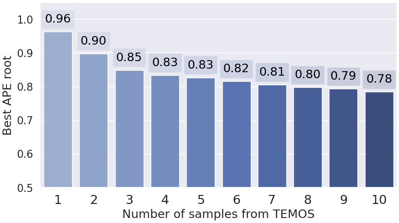
Figure A.1: Best APE root when sampling multiple generations: Given a textual description, we generate multiple different motions, and select the motion that matches best to the ground truth sequence. We show that by sampling more generated sequences per text, we can reduce the APE root metric error.

0.A.3 Number of Transformer layers

Here, we present two different experiments. The first experiment is to change globally the number of layers and the number of heads of all our Transformers. In Table A.3, we see that the results are optimal when they are both fixed at 6, which is used in all other experiments.

Next, in Table A.4, we experiment with a lighter model on top of the DistilBERT text encoder, by adding fewer layers and heads than 6. We see that 1 or 2 layers are not sufficient, but beginning with 4, the results are satisfactory. We use 6 layers in our model.

0.A.4 Pretrained language models

Table A.5: Language model: We experiment with language models larger than DistilBERT and do not observe significant changes in the performance.

Language model	Average Positional Error $\downarrow$				Average Variance Error $\downarrow$
	root joint	global traj.	mean local	mean global	root joint	global traj.	mean local	mean global
DistilBERT [48]	0.963	0.955	0.104	0.976	0.445	0.445	0.005	0.448
BERT [9]	0.986	0.977	0.105	1.000	0.441	0.441	0.005	0.444
RoBERTa [32]	1.066	1.056	0.107	1.079	0.492	0.491	0.005	0.494

We experiment with replacing DistilBERT [48] with a larger pretrained language model. We compare with the original BERT [9] model as well as the more recent RoBERTa [32] model. The results are similar and suggest that DistilBERT is sufficient for this task, while having fewer parameters.

0.A.5 Sampling multiple motions

Given a text input, instead of generating a single motion as in previous methods [2, 14, 30], we can generate multiple motions. As demonstrated in Table 2 of the main paper, we can improve the evaluation metrics by picking the best out of a set of motion generations, that is closest to the ground truth. In Figure A.1, we plot the reduction in APE root error as we increase the number of generations per text from 1 to 10, and observe a monotonic decrease as expected.

Furthermore, we measure the worst case scenario, where we generate 10 motions per text and record the error between the ground truth motion and the most different generated motion out of the 10. We obtain an APE of 1.24 (instead of 0.78 in the best case scenario, and 0.96 in the random scenario). Note that calling this worst case may not be accurate since the single ground truth motion does not represent the only possible motion, i.e., our generations may correspond well to the text without being close to the ground truth joints.

0.A.6 Quantitative results with the SMPL model

To evaluate quantitatively our SMPL-based model, and obtaining results comparable with the MMM framework, we extract the most similar skeleton subset from the SMPL-H joints (provided by AMASS). The correspondence can be found in Table A.6.

Table A.6: Correspondence between the SMPL-H joints and the MMM framework joints.

Type	Joints
MMM	root	BP	BT	BLN	BUN	LS	LE	LW	RS	RE	RW
SMPL-H	pelvis	spine1	spine3	neck	head	left_shoulder	left_elbow	left_wrist	right_shoulder	right_elbow	right_wrist
MMM	LH	LK	LA	LMrot	LF	RH	RK	RA	RMrot	RF
SMPL-H	left_hip	left_knee	left_ankle	left_heel	left_foot	right_hip	right_knee	right_ankle	right_heel	right_foot

Both in SMPL-H and MMM, the bodies are canonicalized with a standard body shape (robot-style for MMM, and average neutral body for SMPL-H). We further rescale the SMPL joints with a factor of 0.64, to match them with MMM joints. We evaluate the model with and without this rescaling. The performance metrics on KIT_SMPL test set can be found in Table A.7. Performance is comparable to that of MMM-based training when evaluating with rescaled joints. We expect future work to compare against the non-rescaled version when employing the SMPL model to interpret the metrics with respect to real human sizes.

Table A.7: Our results with SMPL model: We evaluate our model trained on the SMPL data against the ground truth of the test set of KIT${}_{\text{SMPL}}$ (joints extracted from the AMASS dataset). The first row shows results after a rescaling (to get skeletons closer to MMM processed joints). The second row shows results with the same set of joints but without the final rescaling. Both results are in meters.

		Average Positional Error $\downarrow$				Average Variance Error $\downarrow$
		root	glob.	mean	mean	root	glob.	mean	mean
Dataset	rescaled	joint	traj.	loc.	glob.	joint	traj.	loc.	glob.
KIT${}_{\text{SMPL}}$	✓	0.698	0.689	0.091	0.712	0.157	0.157	0.004	0.161
KIT${}_{\text{SMPL}}$	✗	1.097	1.077	0.169	1.118	0.384	0.383	0.009	0.393

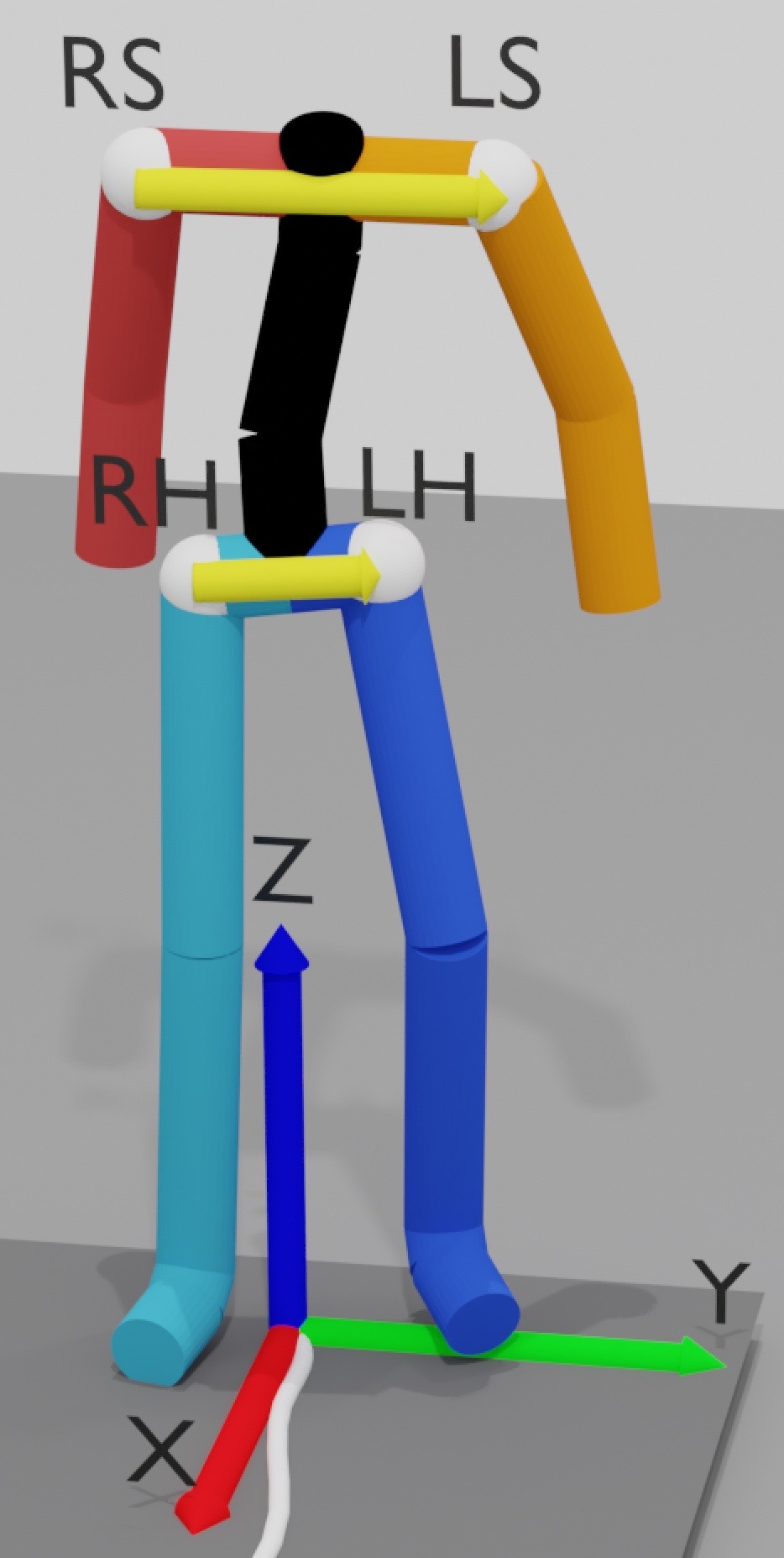
Figure A.2: Body’s local coordinate system: The origin is defined as the projection of the root joint into the ground. The X-axis direction is computed by taking the cross product between the average of the two yellow vectors: (left hip (LH) - right hip (RH)) and (left shoulder (LS) - right shoulder (RS)). The Z-axis (gravity axis) remains the same, and the Y-axis is the cross product of Z and X.

Appendix 0.B Motion representation

Here, we describe in detail the two motion representations employed in this work: skeleton-based (Section 0.B.1) and SMPL-based (Section 0.B.2). We standardize both of them by subtracting the mean and dividing with the standard deviation across the training data.

0.B.1 Skeleton-based representation

We employ the representation introduced by Holden et. al. [21]. As input, we use the 21 joints from the Master Motor Map (MMM) framework [50]. For each frame, we encode:

1. the 3D human joints in a coordinate system local to the body (the definition of the 3 axes and the origin is explained in Figure A.2) without the root joint (20x3=60-dimensional features),

2. the angles between the local X-axis and the global X-axis (by storing them as differences between two frames) (1-dimensional feature),

3. the translation, as the velocity of the root joint in the body’s local coordinate system for X and Y axes, and the position of the root joint for the Z axis (3-dimensional features).

Then, we concatenate this into a feature vector in $\mathbb{R}^{64}$. For a motion sequence of duration $F$, the data sample will be in $\mathbb{R}^{F\times 64}$.

Note that, as we store the difference of angles for ii), when we integrate the angles, we assume that the first angle is 0 (which means that the body’s local coordinate system is aligned with the global one). This is a way of canonicalizing the data so that each sequence starts with the body oriented in the same way.

0.B.2 SMPL-based representation

To construct the feature vector for SMPL data, we store:

1. the SMPL local rotations [33] (parent-relative joint rotation according to the kinematic tree) in the 6D continuous [65] representation (we load the AMASS data processed with SMPL-H [47], but we remove all rotations on the hands, resulting in 21 rotations) (21x6=126-dimensional features),

2. the global rotation in the 6D continuous [65] representation (6-dimensional features),

3. the translation, as the velocity of the root joint in the global coordinate system for the X and Y axes, and the position of the root joint for the Z axis (3-dimensional features).

Then, we concatenate this into a feature vector in $\mathbb{R}^{135}$. For a motion sequence of duration $F$, the data sample will be in $\mathbb{R}^{F\times 135}$.

To help the network learn the global rotation, we canonicalize the global orientation (by rotating all bodies and trajectories) so that the first frame is oriented in the same direction for all sequences.

Appendix 0.C Evaluation details

In this section, we give details on the evaluation metrics and explain our implementation. We further provide details on our human study.

Metrics definitions. As explained in Section 4.1 of the main paper, the metrics are not computed with the original 3D joint coordinates. All motions are first canonicalized (so that the forward direction of the body faces the same direction for all methods and the ground truth). Except for the root joint, all the other joints are expressed in the body’s local coordinate system (see Figure A.2). Then, the APE and AVE metrics are computed separately on these transformed coordinates.

As in JL2P [2] and Ghosh et al. [14], we define the evaluation metrics as follows, and compute them on the test set. The Average Position Error (APE) for a joint $j$ is the average of the L2 distances between the generated and ground-truth joint positions over the time frames ($F$) and test samples ($N$):

$$\operatorname{APE}[j]=\frac{1}{NF}\sum_{n\in N}\sum_{f\in F}\left\|H_{f}[j]-\hat{H}_{f}[j]\right\|_{2}.$$ (4)

We omit denoting the iterator $n$ (over the test set) from the pose $H$ for simplicity. The Average Variance Error (AVE), introduced in Ghosh et al. [14] captures the difference of variations. It is defined as the average of the L2 distances between the generated and ground truth variances for the joint $j$:

$$\operatorname{AVE}[j]=\frac{1}{N}\sum_{n\in N}\|\sigma[j]-\hat{\sigma}[j]\|_{2}$$ (5)

where,

$$\sigma[j]=\frac{1}{F-1}\sum_{f\in F}\left(H_{f}[j]-\widetilde{H}_{f}[j]\right)^{2}\in\mathbb{R}^{3}$$ (6)

denotes the variance of the joint $j$. $\widetilde{H}[j]$ is the mean of the joint throughout the motion.

We report in the tables:

1. the root joint errors by taking the 3 coordinates of the root joint,

2. the global trajectory errors by taking only the X and Y coordinates of the root joint (it is the white trajectory on the ground in the visualizations),

3. the mean local errors by averaging the joint errors in the body’s local coordinate system,

4. the mean global errors by averaging the joint errors in the global coordinate system.

Metrics implementation. We were unable to reuse the evaluation code of Ghosh et al [14] for two reasons: (i) the code did not reproduce the results in [2, 14], (ii) there is a bug in the evaluation script src/eval_APE.py line 249, the slicing for the trajectory loss is wrong (notably y[:, 0] instead of y[:, :, 0]; this issue was confirmed by the authors).

Furthermore, the function fke2rifke might also have slicing bugs (the implementation is the same in the codes of JL2P and Ghosh et al.) and is used indirectly for evaluation metrics.

Finally, the JL2P [2] code release does not include the evaluation. We therefore chose to reimplement our evaluation which we compute directly on 3D coordinates, rather than the standardized (mean subtraction, division by standard deviation) version as explained in Section 4.1 of the main paper.

Perceptual study details. The results of the pairwise comparisons in Figure 3 of the main paper are obtained as follows. We randomly sample 100 test descriptions and generate motion visualizations (as in the supplemental video [41]) from all the three previous methods [2, 14, 30], our method, and the ground truth (500 videos). From these visualizations, we create pairs of videos for each comparison, randomly swapping the left-right order of the video in each question (also 500 videos). For the semantic study, we display the text as well as the pair of videos simultaneously to Amazon Mechanical Turker (AMT) workers. The workers are asked to answer the question: “Which motion corresponds better to the textual description?”. For the realism study, we use the same set of motion pairs and display them to other AMT workers but without showing the text description. They are asked to answer the question: “Which motion is more realistic?”. For both studies, each worker answers a batch of questions, where the first 3 questions are discarded and used as a ‘warmup’ for the task. We further added 2 ‘catch trials’ to detect unqualified workers, whose batch we discarded in our evaluation. We detected exactly 20 such workers out of 100 in both studies. Each pair of videos is shown to multiple workers between 2 and 5 (4 in average), from which we compute a majority vote to determine which generation is better than the other. If there is a tie, we assign a 0.5 equal score to both methods. The resulting percentage is computed over the 100 test descriptions.

For the semantic study, posing the question as a pairwise comparison can lead to a bias towards a more realistic motion (although the semantic correspondence to the text may be worse). To disentangle such realism bias in pairwise comparisons, we repeat the semantic perceptual study with one video at a time: workers on AMT were asked to rate how much they agree with the following statement: “The body motion correctly represents the textual description” by choosing between (1) Strongly disagree, (2) Disagree, (3) Neither agree nor disagree, (4) Agree, or (5) Strongly agree. Using a 20-sequence test set, we generated 4 batches with our method and 1 batch with Ghosh et al. [14]. At the beginning, we added 2 examples along with instructions to explain what we expect from ‘correctness’ and to disentangle from the realism: (i) a realistic motion (from ground truth) that does not correspond to the text, and (ii) a relatively less realistic motion (from generations) that does correspond to the text. We added 4 warm-up examples after them, and 3 catch trials at random locations. We ran the study with 24 AMT workers but half of them failed the catch trials (and the remaining results were not very consistent). So we repeated this experiment with naive lab members. Again we used all the examples at the beginning and catch trials. With this setup, we obtained 21 completed batches. The users rated an average of 3.50 correctness score out of 5 likert scale for our generations versus 3.04 for Ghosh et al. [14]. To further assess the quality of the diverse generations, we generated 5 samples per test description for TEMOS and obtained an average of 3.54 $\pm$ 0.1 score, showing that we preserve correctness within diverse generations as well.

Appendix 0.D Implementation details

Architectural details. For all the encoders and the decoder of TEMOS, we set the embedding dimensionality to 256, the number of layers to 6, the number of heads in multi-head attention to 6, the dropout rate to 0.1, and the dimension of the intermediate feedforward network to 1024 in the Transformers.

Library credits. Our models are implemented with PyTorch [39] and PyTorch Lightning [11]. We use Hydra [55] to handle configurations. For the text models, we use the Transformers library [53].

Runtime. Training our TEMOS model takes about 4.5 hours for 1K epochs, with a batch size of 32, on a single Tesla V100 GPU (16GB) using about 15GB GPU memory for training (i.e., 16 seconds per epoch). In comparison, according to their paper, Ghosh et al. [14] trained their model for 350 epochs on a single Tesla V100 GPU in about 15 hours (i.e., 154 seconds per epoch). While the rest of the hardware specifications or implementation efficiency may vary, given the same type of GPU for both methods, we can expect that our model trains an order of magnitude faster. This may be because our model generates the full motion with only one decoder pass. Previous work produces one frame at a time iteratively (i.e., the next frame has to wait for the previous one to be generated).

Appendix 0.E KIT Motion-Language text statistics

In the KIT Motion-Language [43] dataset, there are 3911 motions and a total of 6352 text sequences (in which 900 motions are not annotated). Using a natural language processing parser, we extract “action phrases” from each sentence, based on verbs. For example, given the sentence “A human walks slowly”, we automatically detect and lemmatize the verb, and attach complements to it, such that it becomes “walk slowly”. With this procedure, we group sequences that correspond to the same action phrase and detect 4153 such action clusters out of 6352 sequences. The distribution of these clusters is very unbalanced: “walk forward” appears 596 times while there are 4030 actions that appear less than 10 times (3226 of them appear only once). On average, an action phrase appears 2.25 times. This information shows that the calculation of distribution-based metrics, such as FID, is not relevant for this dataset.

References

- [1] Ahn, H., Ha, T., Choi, Y., Yoo, H., Oh, S.: Text2Action: Generative adversarial synthesis from language to action. In: International Conference on Robotics and Automation (ICRA) (2018)
- [2] Ahuja, C., Morency, L.P.: Language2Pose: Natural language grounded pose forecasting. In: International Conference on 3D Vision (3DV) (2019)
- [3] Aksan, E., Kaufmann, M., Hilliges, O.: Structured prediction helps 3D human motion modelling. In: International Conference on Computer Vision (ICCV) (2019)
- [4] Bain, M., Nagrani, A., Varol, G., Zisserman, A.: Frozen in time: A joint video and image encoder for end-to-end retrieval. In: International Conference on Computer Vision (ICCV) (2021)
- [5] Bain, M., Nagrani, A., Varol, G., Zisserman, A.: Frozen in time: A joint video and image encoder for end-to-end retrieval. In: International Conference on Computer Vision (ICCV) (2021)
- [6] Barsoum, E., Kender, J., Liu, Z.: HP-GAN: Probabilistic 3D human motion prediction via GAN. In: Computer Vision and Pattern Recognition Workshops (CVPRW) (2018)
- [7] Bhattacharya, U., Childs, E., Rewkowski, N., Manocha, D.: Speech2AffectiveGestures: Synthesizing Co-Speech Gestures with Generative Adversarial Affective Expression Learning (2021)
- [8] Cudeiro, D., Bolkart, T., Laidlaw, C., Ranjan, A., Black, M.: Capture, learning, and synthesis of 3D speaking styles. In: Computer Vision and Pattern Recognition (CVPR) (2019)
- [9] Devlin, J., Chang, M.W., Lee, K., Toutanova, K.: BERT: Pre-training of deep bidirectional transformers for language understanding. In: North American Chapter of the Association for Computational Linguistics (NAACL) (2019)
- [10] Duan, Y., Shi, T., Zou, Z., Lin, Y., Qian, Z., Zhang, B., Yuan, Y.: Single-shot motion completion with transformer. arXiv preprint arXiv:2103.00776 (2021)
- [11] Falcon et al., W.: Pytorch lightning. GitHub. Note: https://github.com/PyTorchLightning/pytorch-lightning (2019)
- [12] Fan, Y., Lin, Z., Saito, J., Wang, W., Komura, T.: Faceformer: Speech-driven 3D facial animation with transformers. In: Computer Vision and Pattern Recognition (CVPR) (2022)
- [13] Gao, T., Dontcheva, M., Adar, E., Liu, Z., Karahalios, K.G.: DataTone: Managing ambiguity in natural language interfaces for data visualization. In: ACM Symposium on User Interface Software & Technology (2015)
- [14] Ghosh, A., Cheema, N., Oguz, C., Theobalt, C., Slusallek, P.: Synthesis of compositional animations from textual descriptions. In: International Conference on Computer Vision (ICCV) (2021)
- [15] Ginosar, S., Bar, A., Kohavi, G., Chan, C., Owens, A., Malik, J.: Learning individual styles of conversational gesture. In: Computer Vision and Pattern Recognition (CVPR) (2019)
- [16] Guo, C., Zuo, X., Wang, S., Zou, S., Sun, Q., Deng, A., Gong, M., Cheng, L.: Action2Motion: Conditioned generation of 3D human motions. In: ACM International Conference on Multimedia (ACMMM) (2020)
- [17] Habibie, I., Holden, D., Schwarz, J., Yearsley, J., Komura, T.: A recurrent variational autoencoder for human motion synthesis. In: British Machine Vision Conference (BMVC) (2017)
- [18] Harvey, F.G., Yurick, M., Nowrouzezahrai, D., Pal, C.: Robust motion in-betweening. ACM Transactions on Graphics (TOG) (2020)
- [19] Henter, G.E., Alexanderson, S., Beskow, J.: MoGlow: Probabilistic and controllable motion synthesis using normalising flows. ACM Transactions on Graphics (TOG) (2020)
- [20] Hill, I.: Natural language versus computer language. In: Designing for Human-Computer Communication (1983)
- [21] Holden, D., Saito, J., Komura, T.: A deep learning framework for character motion synthesis and editing. ACM Transactions on Graphics (TOG) (2016)
- [22] Ionescu, C., Li, F., Sminchisescu, C.: Latent structured models for human pose estimation. In: International Conference on Computer Vision (ICCV) (2011)
- [23] Ionescu, C., Papava, D., Olaru, V., Sminchisescu, C.: Human3.6M: Large scale datasets and predictive methods for 3D human sensing in natural environments. Transactions on Pattern Analysis and Machine Intelligence (TPAMI) (2014)
- [24] Karras, T., Aila, T., Laine, S., Herva, A., Lehtinen, J.: Audio-driven facial animation by joint end-to-end learning of pose and emotion. ACM Transactions on Graphics (TOG) (2017)
- [25] Kingma, D.P., Ba, J.: Adam: A method for stochastic optimization. In: International Conference on Learning Representations (ICLR) (2015)
- [26] Kingma, D.P., Welling, M.: Auto-encoding variational bayes. In: International Conference on Learning Representations (ICLR) (2014)
- [27] Lee, H.Y., Yang, X., Liu, M.Y., Wang, T.C., Lu, Y.D., Yang, M.H., Kautz, J.: Dancing to music. In: Neural Information Processing Systems (NeurIPS) (2019)
- [28] Li, J., Yin, Y., Chu, H., Zhou, Y., Wang, T., Fidler, S., Li, H.: Learning to generate diverse dance motions with transformer. arXiv preprint arXiv:2008.08171 (2020)
- [29] Li, R., Yang, S., Ross, D.A., Kanazawa, A.: AI choreographer: Music conditioned 3D dance generation with AIST++. In: International Conference on Computer Vision (ICCV) (2021)
- [30] Lin, A.S., Wu, L., Corona, R., Tai, K., Huang, Q., Mooney, R.J.: Generating animated videos of human activities from natural language descriptions. Visually Grounded Interaction and Language (ViGIL) NeurIPS Workshop (2018)
- [31] Lin, X., Amer, M.: Human motion modeling using DVGANs. arXiv preprint arXiv:1804.10652 (2018)
- [32] Liu, Y., Ott, M., Goyal, N., Du, J., Joshi, M., Chen, D., Levy, O., Lewis, M., Zettlemoyer, L., Stoyanov, V.: Roberta: A robustly optimized BERT pretraining approach. arXiv preprint arXiv:1907.11692 (2019)
- [33] Loper, M., Mahmood, N., Romero, J., Pons-Moll, G., Black, M.J.: SMPL: A skinned multi-person linear model. ACM Transactions on Graphics (TOG) (2015)
- [34] Loshchilov, I., Hutter, F.: Decoupled weight decay regularization. In: International Conference on Learning Representations (ICLR) (2019)
- [35] Mahmood, N., Ghorbani, N., Troje, N.F., Pons-Moll, G., Black, M.J.: AMASS: Archive of motion capture as surface shapes. In: International Conference on Computer Vision (ICCV) (2019)
- [36] Mandery, C., Terlemez, O., Do, M., Vahrenkamp, N., Asfour, T.: The kit whole-body human motion database. In: International Conference on Advanced Robotics (ICAR) (2015)
- [37] Martinez, J., Black, M.J., Romero, J.: On human motion prediction using recurrent neural networks. In: Computer Vision and Pattern Recognition (CVPR) (2017)
- [38] Mikolov, T., Sutskever, I., Chen, K., Corrado, G.S., Dean, J.: Distributed representations of words and phrases and their compositionality. In: Neural Information Processing Systems (NeurIPS) (2013)
- [39] Paszke, A., Gross, S., Massa, F., Lerer, A., Bradbury, J., Chanan, G., Killeen, T., Lin, Z., Gimelshein, N., Antiga, L., Desmaison, A., Kopf, A., Yang, E., DeVito, Z., Raison, M., Tejani, A., Chilamkurthy, S., Steiner, B., Fang, L., Bai, J., Chintala, S.: PyTorch: An imperative style, high-performance deep learning library. In: Neural Information Processing Systems (NeurIPS) (2019)
- [40] Pavllo, D., Grangier, D., Auli, M.: QuaterNet: A quaternion-based recurrent model for human motion. In: British Machine Vision Conference (BMVC) (2018)
- [41] Petrovich, M., Black, M.J., Varol, G.: TEMOS project page: Generating diverse human motions from textual descriptions. https://mathis.petrovich.fr/temos/
- [42] Petrovich, M., Black, M.J., Varol, G.: Action-conditioned 3D human motion synthesis with transformer VAE. In: International Conference on Computer Vision (ICCV) (2021)
- [43] Plappert, M., Mandery, C., Asfour, T.: The KIT motion-language dataset. Big Data (2016)
- [44] Plappert, M., Mandery, C., Asfour, T.: Learning a bidirectional mapping between human whole-body motion and natural language using deep recurrent neural networks. Robotics Auton. Syst. (2018)
- [45] Radford, A., Kim, J.W., Hallacy, C., Ramesh, A., Goh, G., Agarwal, S., Sastry, G., Askell, A., Mishkin, P., Clark, J., Krueger, G., Sutskever, I.: Learning transferable visual models from natural language supervision. In: International Conference on Machine Learning (ICML) (2021)
- [46] Richard, A., Zollhöfer, M., Wen, Y., de la Torre, F., Sheikh, Y.: Meshtalk: 3D face animation from speech using cross-modality disentanglement. In: International Conference on Computer Vision (ICCV) (2021)
- [47] Romero, J., Tzionas, D., Black, M.J.: Embodied hands: Modeling and capturing hands and bodies together. ACM Transactions on Graphics (TOG) (2017)
- [48] Sanh, V., Debut, L., Chaumond, J., Wolf, T.: DistilBERT, a distilled version of BERT: smaller, faster, cheaper and lighter. arXiv preprint arXiv:1910.01108 (2019)
- [49] Saunders, B., Camgoz, N.C., Bowden, R.: Mixed SIGNals: Sign language production via a mixture of motion primitives. In: International Conference on Computer Vision (ICCV) (2021)
- [50] Terlemez, O., Ulbrich, S., Mandery, C., Do, M., Vahrenkamp, N., Asfour, T.: Master motor map (MMM) — framework and toolkit for capturing, representing, and reproducing human motion on humanoid robots. In: International Conference on Humanoid Robots (2014)
- [51] University, C.M.: CMU MoCap Dataset
- [52] Vaswani, A., Shazeer, N., Parmar, N., Uszkoreit, J., Jones, L., Gomez, A.N., Kaiser, L., Polosukhin, I.: Attention is all you need. In: Neural Information Processing Systems (NeurIPS) (2017)
- [53] Wolf, T., Debut, L., Sanh, V., Chaumond, J., Delangue, C., Moi, A., Cistac, P., Rault, T., Louf, R., Funtowicz, M., Davison, J., Shleifer, S., von Platen, P., Ma, C., Jernite, Y., Plu, J., Xu, C., Scao, T.L., Gugger, S., Drame, M., Lhoest, Q., Rush, A.M.: Transformers: State-of-the-art natural language processing. In: Empirical Methods in Natural Language Processing: System Demonstrations (2020)
- [54] Xu, J., Mei, T., Yao, T., Rui, Y.: MSR-VTT: A large video description dataset for bridging video and language. In: Computer Vision and Pattern Recognition (CVPR) (2016)
- [55] Yadan, O.: Hydra - a framework for elegantly configuring complex applications (2019), https://github.com/facebookresearch/hydra
- [56] Yamada, T., Matsunaga, H., Ogata, T.: Paired recurrent autoencoders for bidirectional translation between robot actions and linguistic descriptions. Robotics and Automation Letters (2018)
- [57] Yan, S., Li, Z., Xiong, Y., Yan, H., Lin, D.: Convolutional sequence generation for skeleton-based action synthesis. In: International Conference on Computer Vision (ICCV) (2019)
- [58] Yang, J., Li, C., Zhang, P., Xiao, B., Liu, C., Yuan, L., Gao, J.: Unified contrastive learning in image-text-label space. In: Computer Vision and Pattern Recognition (CVPR) (2022)
- [59] Yuan, L., Chen, D., Chen, Y., Codella, N., Dai, X., Gao, J., Hu, H., Huang, X., Li, B., Li, C., Liu, C., Liu, M., Liu, Z., Lu, Y., Shi, Y., Wang, L., Wang, J., Xiao, B., Xiao, Z., Yang, J., Zeng, M., Zhou, L., Zhang, P.: Florence: A new foundation model for computer vision. arXiv preprint arXiv:2111.11432 (2021)
- [60] Yuan, Y., Kitani, K.: Dlow: Diversifying latent flows for diverse human motion prediction. In: European Conference on Computer Vision (ECCV) (2020)
- [61] Zanfir, A., Bazavan, E.G., Xu, H., Freeman, W.T., Sukthankar, R., Sminchisescu, C.: Weakly supervised 3D human pose and shape reconstruction with normalizing flows. In: European Conference on Computer Vision (ECCV) (2020)
- [62] Zhang, Y., Black, M.J., Tang, S.: Perpetual motion: Generating unbounded human motion. arXiv preprint arXiv:2007.13886 (2020)
- [63] Zhang, Y., Black, M.J., Tang, S.: We are more than our joints: Predicting how 3D bodies move. In: Computer Vision and Pattern Recognition (CVPR) (2021)
- [64] Zhao, R., Su, H., Ji, Q.: Bayesian adversarial human motion synthesis. In: Computer Vision and Pattern Recognition (CVPR) (2020)
- [65] Zhou, Y., Barnes, C., Lu, J., Yang, J., Li, H.: On the continuity of rotation representations in neural networks. In: Computer Vision and Pattern Recognition (CVPR) (2019)