Adversarial Distortion Learning for Medical Image Denoising

Abstract

We present a novel adversarial distortion learning (ADL) for denoising two- and three-dimensional (2D/3D) biomedical image data. The proposed ADL consists of two auto-encoders: a denoiser and a discriminator. The denoiser removes noise from input data and the discriminator compares the denoised result to its noise-free counterpart. This process is repeated until the discriminator cannot differentiate the denoised data from the reference. Both the denoiser and the discriminator are built upon a proposed auto-encoder called Efficient-Unet. Efficient-Unet has a light architecture that uses the residual blocks and a novel pyramidal approach in the backbone to efficiently extract and re-use feature maps. During training, the textural information and contrast are controlled by two novel loss functions. The architecture of Efficient-Unet allows generalizing the proposed method to any sort of biomedical data. The 2D version of our network was trained on ImageNet and tested on biomedical datasets whose distribution is completely different from ImageNet; so, there is no need for re-training. Experimental results carried out on magnetic resonance imaging (MRI), dermatoscopy, electron microscopy and X-ray datasets show that the proposed method achieved the best on each benchmark. Our implementation and pre-trained models are available at https://github.com/mogvision/ADL.

Adversarial networks, Deep learning, Deep neural network, Image denoising

1 Introduction

Image denoising aims to recover latent noise-free two/three-dimensional (2D/3D) image data $\mathbf{x}$ from its noisy counterpart $\mathbf{y}=\mathbf{x}+\mathbf{n}$, where $\mathbf{n}$ denotes noise that is independent with respect to $\mathbf{x}$. The denoising problem tends to be an ill-posed inverse problem as no unique solution exists. Denoising is an essential preprocessing step in many medical imaging applications. A vast number of methods have been proposed over the past decades [9, 30, 17, 38], and recently, methods based on deep neural networks (DNNs) attract more attention due to their good performance [12, 52, 40, 26, 54].

For additive noise, it is possible to establish the Bayesian approach, where the posterior $P_{x|y}(\mathbf{x}|\mathbf{y})$ is a combination of the data likelihood $P_{y|x}(\mathbf{y}|\mathbf{x})$ and a prior model $P_{x}(\mathbf{x})$, i.e.:

$$\mathbf{\hat{x}}=\operatorname*{argmax}_{\mathbf{x}}\;P_{x|y}(\mathbf{x}|\mathbf{y})\\ =\operatorname*{argmax}_{\mathbf{x}}\;\text{log}\>P_{y|x}(\mathbf{y}|\mathbf{x})+\text{log}\>P_{\mathbf{x}}(\mathbf{x}).$$ (1)

The denoising problem Eq.  1 can be also expressed as an optimization of a data term penalized by one or more regularization terms as follows:

$$\mathbf{\hat{x}}=\operatorname*{argmin}_{\mathbf{x}}\>\left\|\mathbf{y}-\mathbf{x}\right\|^{p}_{p}+\lambda\mathcal{R}(\mathbf{x}),$$ (2)

where $\left\|.\right\|_{p}$ denotes the $\ell{p}$-norm, $1\leq p\leq 2$. $\mathcal{R}$ poses penalty terms on the unknown latent $\mathbf{x}$ which is associated with the prior term $P_{x}(\mathbf{x})$ defined in Eq. 1. $\lambda$ is a Lagrangian parameter, which can be determined manually or automatically [4, 45]. In general, the denoising methods can be divided into model- and learning-based categories. The model-based approach solves Eq. 2 using one or several regularization terms [10, 28, 27, 56]. In the learning-based approach, a model can learn features with supervision [8, 34] or it may learn the features simultaneously during image reconstruction [36]. Recently, the deep learning-based approaches [12, 25, 23] have reached excellent performance in denoising biomedical images by training DNNs on paired or unpaired images of target clean and noisy data. Despite the success of the existing denoising techniques, the contents of denoised images by such methods still suffer from poor preservation of texture and contrast. Requiring prior knowledge of noise and the lack of generalizability to various types of biomedical image data are other limitations of the current techniques.

In this study, we propose an adversarial distortion learning-based (ADL) method that does not require any prior knowledge about the noise in images. ADL is a supervised feature learning method that is comprised of a denoiser and a discriminator that iteratively optimizes each other to find high-quality denoised contents. Both the denoiser and the discriminator are built upon a novel network called Efficient-Unet. Efficient-Unet has a light architecture with pyramidal residual blocks backbone that enforces the higher-level features are in consonance with each other hierarchically. A remarkable feature of our approach is that it can be used for denoising any type of 2D/3D biomedical image data with no need for re-training. The light architecture of the proposed method allows a fast evaluation of test data and it considerably reduces the computational time of the conventional model-based approaches. The key contributions of this study are as follows:

• We design a novel pyramidal learning scheme, named Efficient-Unet, to further participate high-level features in the output results during training. Efficient-Unet does not need training data whose distribution is close to that of the test data, so improving the generalizability of the proposed network.

• We introduce a novel pyramidal loss function using ‘algorithme à trous’ (ATW) [42]. The proposed loss function keeps textural information of the reference data without amplifying noise’s side effects in non-textured regions.

• To preserve the histograms of reference images, we propose a novel histogram-based loss function for improving the appearance contents of denoised images.

• We provide both 2D and 3D networks of our method for denoising any sort of 2D/3D biomedical image data.

Experimental results show that the proposed ADL achieves state-of-the-art results on all the benchmarks alongside solving overfitting, generalizability to any sort of biomedical data, and computational burdens.

2 Related Work

Medical image denoising approaches can be grouped into two subcategories: model-based and learning-based methods. In the model-based approach, optimization of Eq. 1 with respect to the likelihood term only is typically ill-posed, so needs one or more regularization terms alongside the data fidelity term to find and stabilize the denoised outputs. Thus far, a wide range of model-based techniques have been developed, ranging from total variation (TV) regularizers [10, 56, 41] to non-local self-similarity regularizers [28, 7, 27, 20, 9, 30, 5]. TV-based regularization terms can successfully recover piecewise constant images but cause several artifacts to complex images with rich edges and textures. Since natural images tend to contain repetitive edge and textural information, combination of non-local self-similarity [28, 7, 27, 20] with the sparse representation [34] and low-rank approximation [3] lead to significant improvements over their local counterparts. The regularization terms play an important role in the quality of resultant denoised images. Despite the acceptable performance of the model-based methods in image denoising, there are still several drawbacks with these techniques. Requiring a specific model for a single denoising task, lack of generalizability to various types of data, or the need for manually or semi-automatically tuning parameters are the challenging that is still required to be addressed. Moreover, the non-local self-similarity-based methods iteratively optimize Eq. 2 so their convergence often needs considerable time.

A learning-based method aims at learning the parameters of a model with available datasets. Sparsity-based techniques are well-studied learning approaches, which represent local image structures with a few elemental structures so-called atoms from an off-the-shelf transformation matrix-like Wavelets [14] or a learned dictionary [51, 36]. In recent years, deep learning methods have been widely used for the enhancement of biomedical images, ranging from MRI [25, 43], CT [52, 50], X-ray [12], to electron microscopy (EM) [35, 22]. The learning process of DNNs can be categorized into supervised [55, 40, 24] or unsupervised [57, 2, 22] approaches. Supervised learning DNNs consider clean and noisy image pairs for training where the noisy counterparts are obtained through adding synthesized noise to the target clean ones. To overcome the lack of availability of sufficient clean data for training, unsupervised methods [57, 16, 22] have been developed that estimate the map of noise from unpaired images, leveraging the supervision of clean targets. Unsupervised techniques often explore the noise map by generative adversarial networks (GANs) [13] and its variants like conditional GAN [31] or CycleGAN [57]. Typically, the supervised DNNs have shown superior performance over the unsupervised and conventional model-based approaches. Despite the great success of DNNs in denoising biomedical images, the contents of denoised images still suffer from poor textural information. Although several works [24, 40] show less tendency toward overfitting and being data-driven, their performance is still highly dependent on the training samples. Since clean biomedical images for training are not available or available only in very limited quantities, this aspect of the current DNN techniques limits their generalizability to different sorts of biomedical images.

3 Proposed Method

The intuition of ADL is that the representation of images must be robust against random phenomena like noise. ADL consists of a denoiser and a discriminator, where both have the same Unet-like architecture called Efficient-Unet. There is some minor difference between the Efficient-Unet of the denoiser and that of the discriminator (Section 3.1). ADL is trained by minimizing competing multiscale objectives between the denoiser and the discriminator. During training, we enforce the networks on keeping the edges, histogram, and paramedical information of the reference/ground-truth data. The proposed loss functions are detailed in Section 3.2.

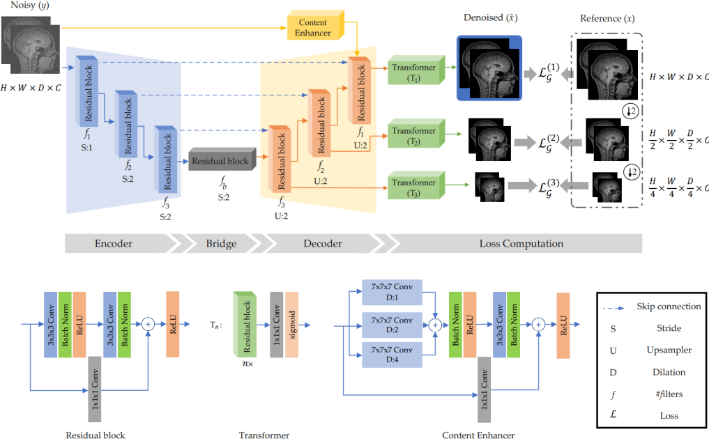
Figure 1: Framework of the Efficient-Unet for denoiser with the training steps. Efficient-Unet is composed of the encoder, decoder, and Content Enhancer blocks. The output of the decoder at every scale is mapped into the image domain by a Transformer block. We then enforce consistency between the outputs of the decoder and their counterparts $x$. Low-level features further contribute into the denoised image by the Content Enhancer block. When the noise level is low, the filters of this block are activated improving the convergence with no need for high-level features.

3.1 Efficient-Unet

Let $\mathbf{x}\in\mathbb{R}^{H\times W\times D\times C}$ ($\mathbf{x}\in\mathbb{R}^{H\times W\times C}$ for 2D) be the noise-free 3D (/2D) image data, and $\mathbf{y}\in\mathbb{R}^{H\times W\times D\times C}$ the observed image data that is generated by adding WGN of standard deviation ($\sigma$) to its noise-free counterpart $\mathbf{x}$. During training, $\mathbf{x}$ plays as a reference, noise level $\sigma$ is unknown, and the goal is to recover $\mathbf{y}$ from $\mathbf{x}$. Efficient-Unet and the training architecture for learning network parameters of the proposed denoiser is depicted in Fig. 1. Efficient-Unet consists of an encoder, a bridge, a decoder, a content enhancer, and transformers. Similarly, the framework of Efficient-Unet for the discriminator is depicted in Fig. 2.

The encoder unit is comprised of three consecutive residual blocks with strides one and two (denoted by $S$ in Fig. 1) that extracts the features from the observed data. The number of filters in the encoder layers is doubled after each downsampling operation (i.e., $S=2$). Several studies[15, 55, 40] have shown the effectiveness of residual blocks in deep learning. We use the residual blocks in our auto-encoder structure for effective denoiser prior modeling. To have large activation maps, we delayed the downsampling of the first layer, where its stride is 1. The extracted features by the encoder are then passed through a bridge with $f_{b}$ filters followed by the decoder unit that provides an estimation of the denoised input data $\mathbf{\hat{x}}$ in the feature domain. The features of each decoder layer are mapped into the image domain by the transformer unit $T_{n}$ where $n$ is the index of the corresponding layer. The transformer unit is a set of $n$ residual blocks followed by a $1\times 1\times 1$ convolution and a sigmoid activation layers. The number of filters in the transformer layers is halved $n$ times and the filter size of $1\times 1\times 1$ convolution layer is equal to $C$, which is the number of input channels. Throughout this paper, the kernel size and dilation of the convolutional layers are 3 and 1, respectively, unless otherwise noted.

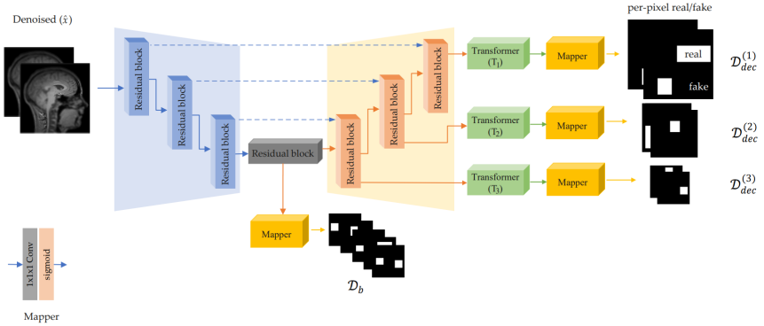
Figure 2: Framework of the proposed Efficient-Unet for discriminator with the training steps.

Thus far, the only difference between the Efficient-Unet of the denoiser and that of the discriminator is the filter size of convolution layers, i.e. $\{f_{1},f_{2},f_{3},f_{b}\}$. It is set as $\{96,128,160,192\}$ for the denoiser and $\{48,64,80,96\}$ for the discriminator. The discriminator network needs a lower number of learning parameters compared to the denoiser because the discriminator is a classifier that computes the loss for misclassifying a noise-free instance as noisy or a noisy instance as noise-free. Since the discriminator is a classifier, the output of each transformer is mapped into a binary mask by a mapper which is shown in Fig. 2. The mapping layer is comprised of convolution layers with a filter size of 1 followed by a sigmoid activation layer to map the input to a binary mask. The denoiser has also one extra unit called content enhancer and it is designed to preserve the sparse information like edges and textures that are not or less affected by noise. As shown in Fig. 1, the content enhancer is a residual block, wherein the first layer extracts features by three different dilation values, $D$. Several studies [11, 42] have shown that the structural information, which is mainly edges and textures, exists at different scales. So we consider three convolutions of strides 1, 2, and 4 to extract such features from the input noisy data directly. In the absence of noise, this unit has more activated layers. The content enhancer layer is concatenated by the last layer of the decoder before feeding $T_{1}$. The denoised data $\mathbf{\hat{x}}$ is the output of layer $T_{1}$, shown by a blue rectangle in Fig. 1. It is also worth mentioning that the bias parameter in the proposed Efficient-Unet is deactivated since bias-free networks increase the linearity property by canceling the bias parameter [32]. Moreover, when the magnitude of the bias is much larger than that of filters, the generalizability of the model is limited so less prone to overfitting [54].

3.2 Multiscale loss functions

ADL consists of two auto-encoders: a denoiser $\mathcal{G}$ and a discriminator $\mathcal{D}$. Generally, the parameters of adversarial nets are optimized by minimizing a two-player game in an alternating manner [13]:

$$\begin{array}[]{l}\mathcal{L_{D}}\mathrel{\ensurestackMath{\stackon[1pt]{=}{\scriptstyle\Delta}}}-\mathbb{E}_{\mathbf{x}}\{\text{log}\;\mathcal{D}(\mathbf{x})\}-\mathbb{E}_{\mathbf{y}}\{\text{log}\left(1-\mathcal{D}(\mathcal{G}(\mathbf{y}))\right)\},\\ \mathcal{L_{G}}\mathrel{\ensurestackMath{\stackon[1pt]{=}{\scriptstyle\Delta}}}-\mathbb{E}_{\mathbf{y}}\{\text{log}\;\mathcal{D}(\mathcal{G}(\mathbf{y}))\}.\end{array}$$ (3)

Denoiser $\mathcal{G}$ aims to estimate a clean image while discriminator $\mathcal{D}$ distinguishes between reference $\mathbf{x}$ and denoised ${\mathcal{G}(\mathbf{y})}$ instances. Eq. (3) does not maintain textural, global, and local data representation. To this end, we propose novel multiscale loss functions for both the denoiser and the discriminator. We minimize the loss of denoiser from coarse to fine resolution for enforcing the participation of the decoder’s features in the resultant high-resolution denoised image. Likewise, we enforce the discriminator network to discriminate the target and the denoised images from bottom to top. Moving from coarse resolution towards fine one enhances structural features at the corresponding resolution, resulting in rich edge and textural information in the denoised data.

3.2.1 Denoiser’s loss function ($\mathcal{L_{G}}$)

We define the loss function of the denoiser as a combination of an ${\ell_{1}}$ loss (denoted by $\mathcal{L}_{\ell_{1}}$), a novel pyramidal textural loss $\mathcal{L}_{pyr}$, and a novel histogram loss $\mathcal{L}_{{H}ist}$ that are weighted by $\lambda_{\ell_{1}}$, $\lambda_{p}$, and $\lambda_{\mathcal{H}}$, respectively:

$$\mathcal{L_{G}}\mathrel{\ensurestackMath{\stackon[1pt]{=}{\scriptstyle\Delta}}}\lambda_{\ell_{1}}\mathcal{L}_{\ell_{1}}+\lambda_{p}\mathcal{L}_{pyr}+\lambda_{\mathcal{H}}\mathcal{L}_{\mathcal{H}ist}\\ =-\mathbb{E}{\{\mid\mathcal{G}(\mathbf{y})-\mathbf{x}\mid}\}-\lambda_{p}\mathbb{E}\Big{\{}\sum_{j=1}^{J}\mid\Delta_{j}.\mathcal{G}(\mathbf{y})-\Delta_{j}.\mathbf{x}\mid\Big{\}}\\ -\lambda_{\mathcal{H}}\mathbb{E}\{\text{logcosh}\big{(}\mathcal{H}\left[\mathbf{\mathcal{G}(\mathbf{y})}\right]-\mathcal{H}\left[\mathbf{x}\right]\big{)}\}.$$ (4)

• $\mathbf{\mathcal{L}_{\ell_{1}}}$: The data fidelity is an $\ell_{1}$-norm between the denoised and reference instances. Compared to the $\ell_{2}$-norm, the $\ell_{1}$-norm is more robust against outliers.

• $\mathbf{\mathcal{L}_{pyr}}$: The pyramidal textural loss aims at preserving edges and texture in to-be-denoised images. Unlike the conventional edge-preserving regularization terms like TV and its variants [33, 48] that compute the differential of given noisy images, our goal is to measure the textural difference between to-be-denoised images and their corresponding reference only. Traditional TVs use first-, second- or higher order-based derivative operators to filter noisy images. The main drawback of such operators is to boost the pixels with high-level noise so it may bias the loss towards dominant values. For this reason, the images denoised by TV-like regularisation terms are often accompanied by smoothness in both textural and non-textural regions. To cope with this problem, we introduce a pyramidal loss function using ATW [42]. ATW is a stationary Wavelet transform that decomposes an image into several levels by a cubic spline filter and then subtracts any two successive layers to obtain fine images with edges and texture. The low-pass filters in ATW alleviate the side effects of noise so it enables us to include texture information of input images in the loss function. Fig. 3 briefs ATW. In short, it decomposes an input image into $J$ levels by a cubic spline finite impulse response that is denoted by $h^{(1)}$. Unlike the non-stationary multiscale transforms that downscale the images and then apply a filter, ATW upscales the kernel by inserting ‘$2^{j-1}-1$’ zeros between each pair of adjacent elements in $h^{(1)}$, where $j$ denotes the $j$-th decomposition level. Fine images with texture and edges are derived via subtraction of any two successive filtered images. Further details can be found in [42, 11]. In Eq. 4 $\Delta_{j}.$ denotes the textural image at the $j$-th level derived by ATW. $J$ is a positive integer that denotes the number of decomposition levels. Typically, four decomposition levels ($J=4$) have been able to extract the majority of edges and texture laid in a wide range of sigma values [11].

• $\mathbf{\mathcal{L}_{\mathcal{H}ist}}$: The histogram loss assures that the histograms of $\mathcal{G}(\mathbf{y})$ and $\mathbf{x}$ are close to each other. This term maintains the global structure of $\mathcal{G}(\mathbf{y})$ with respect to $\mathbf{x}$ since the added edges and texture information (by ATW) may change the overall histogram of the denoised instance. To compute this loss, we first compute the histogram of both $\mathcal{G}(\mathbf{y})$ and $\mathbf{x}$ denoted by $\mathcal{H}$. Then, we use an strictly increasing function that computes the loss between $\mathcal{H}\left[\mathbf{\mathcal{G}(\mathbf{y})}\right]$ and $\mathcal{H}\left[\mathbf{x}\right]$. To this end, we use ‘$\text{logcosh}(p)=\text{log(cosh(}p\text{))}$’ that is approximately equal to $\frac{p^{2}}{2}$ for small $p$ and to $\text{log}(p)-\text{log}(2)$ for large $p$. It is worth noting that here we use the histogram loss for preserving the global structure between the denoised image and its reference, and this is different from other histogram works like [58, 44]. In [58], a gradient histogram is used for texture preservation, and Delbracio et al. [44] proposed a DNN-based histogram as a fidelity term.

In Efficient-Unet, features at fine-resolution maps are reconstructed from its coarser ones (Fig. 1). Thus, an inefficiency in coarser spatial scales (or equivalently, higher-level feature maps) may yield poor resultant feature maps. To cope with this problem, we propose a pyramidal version of the loss function defined in Eq. 4 that keeps the consistency between $\mathcal{G}(\mathbf{y})$ and its counterpart $\mathbf{x}$ at each spatial scale. To compute the proposed multiscale loss, we generalize the transformer unit, introduced in Section 3.1, to lower spatial scales (here, two scales $T_{2}$ and $T_{3}$) and then get the corresponding denoised image data. Then, we compute the loss function presented in Eq. 4 at every scale and finally take an average of the losses to yield the denoiser loss:

$$\mathcal{L_{G}}=\sum_{s=1}^{3}(\lambda_{\ell_{1}}\mathcal{L}^{(s)}_{\ell_{1}}+\lambda_{e}\mathcal{L}^{(s)}_{edge}+\lambda_{\mathcal{H}}\mathcal{L}^{(s)}_{\mathcal{H}ist}),$$ (5)

where superscript $s$ denotes the scale of the data pyramid and the total number of scales is set to 3 in the study.

3.2.2 Discriminator’s loss function ($\mathcal{L_{D}}$)

Most discriminators are based on an encoder that determines whether the input instance is fake or real. Schonfeld et al. [39] have shown that using an Unet structure for discriminator could increase the performance of the generator (here, the denoiser). Borrowed the same concepts from [39] and similar to Eq.5, we propose the following loss function for the discriminator (see Fig. 2):

$$\mathcal{L_{D}}=\mathcal{L}_{\mathcal{D}_{b}}+\sum_{s=1}^{3}\mathcal{L}^{(s)}_{\mathcal{D}_{dec}},$$ (6)

where $\mathcal{L}_{\mathcal{D}_{b}}$ is the bridge loss and it is defined as

$$\mathcal{L}_{\mathcal{D}_{b}}=-\mathbb{E}\Big{\{}\sum_{m,n}\text{min}(0,-1+{\mathcal{D}_{b}}(\mathbf{x})\big{|}_{m,n}\Big{\}}-\\ \mathbb{E}\Big{\{}\sum_{m,n}\text{min}(0,-1-{\mathcal{D}_{b}}(\mathbf{\hat{x}})\big{|}_{m,n}\Big{\}}.$$ (7)

Here, subscripts $\{m,n\}$ denote discriminator decision at pixel $(m,n)$. Likewise, $\mathcal{L}_{\mathcal{D}_{dec}}$ in Eq. 6 is defined as follows:

$$\mathcal{L}^{(s)}_{\mathcal{D}_{dec}}=-\mathbb{E}\Big{\{}\sum_{m,n}\text{min}(0,-1+{\mathcal{D}_{dec}}(\mathbf{x})\big{|}_{m,n}\Big{\}}-\\ \mathbb{E}\Big{\{}\sum_{m,n}\text{min}(0,-1-{\mathcal{D}_{dec}}(\mathbf{\hat{x}})\big{|}_{m,n}\Big{\}},\>s\in\{1,2,3\}.$$ (8)

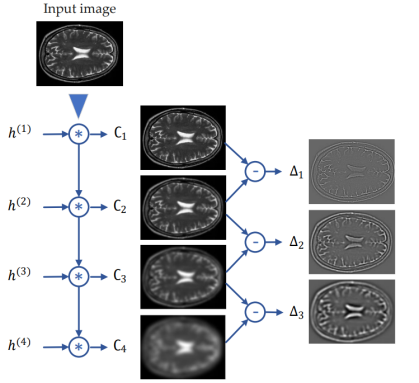
Figure 3: ATW decomposition for image data. Since 2D kernel $h$ is separable, the ATW decomposition for 3D image data is obtained by convolving three 1D cubic kernels in the x, y, and z directions. ATW is comprised of inherently low-pass filters that attenuate the side effects of noise.

3.3 Training details

We implemented ADL for both 2D and 3D data. To show the generalizability of the denoiser, we trained the 2D model on ImageNet [37], whose data distribution is different from that of biomedical images. The training and the validations sets contain 1,281,168 and 50,000 images of size $224\times 224$, respectively. The denoiser model was trained on color and gray-scale images separately. We augmented the data by rotation, $\theta\in\{90^{\circ},180^{\circ},270^{\circ}\}$, and flips. We added zero-mean WGN to input images with $\sigma$ that was randomly selected in interval [0,55]. The noisy images were not clipped into the interval [0,255], making sure that the distribution of added noise was still WGN. The 3D model was trained on the IXI Dataset , containing approximately 570 8-bit T1, T2 and PD-weighted MR images acquired at three different hospitals in London: Hammersmith Hospital using a Philips 3T system, Guy’s Hospital using a Philips 1.5T system, and Institute of Psychiatry using a GE 1.5T system. The size of MRI volumes is 256$\times$256$\times n$, where $n\in[28,150]$. We randomly cropped the volumes into sub-volumes of 128$\times$128$\times$48 to facilitate the training. we added zero-mean white Gaussian ($\sigma\in[0,55]$), Rician ($\sigma\in[0,25]$ and $\nu\in[0,15]$), and Rayleigh ($\sigma\in[0,25]$) noise to input MRI volumes. Likewise to the 2D training, the values of the parameters in the above-mentioned intervals were randomly selected . We used the Adam algorithm [19] as an optimizer with the ReduceLRonPlateau scheduler [47]. The optimization started with a learning rate of $10^{-4}$ and it was reduced (by the ReduceLRonPlateau scheduler) until the PSNR of validation has stopped improving. The weights in Eq. 5, i.e. $\{\lambda_{\ell_{1}}$, $\lambda_{e}$, $\lambda_{\mathcal{H}}\}$, were set to 1.

Reproducibility: The reference implementation of ADL is based on TensorFlow. All the experiments were conducted on 4 A-100 GPUs. The implementation and pre-trained models are available at https://github.com/mogvision/ADL. We also provided PyTorch and Colab implementation of ADL on the GitHub.

Table 1: PSNR (dB) and SSIM results (average $\pm$ standard deviation) of different method on the image-based datasets for noise levels 10, 15, 25, 35, 50. The best and second best results are highlighted in boldface and in italic, respectively.

Dataset	Noise Level			PSNR $\uparrow$					SSIM $\uparrow$
		BM3D	DRAN	DnCNN-S	SwinIR	ADL	BM3D	DRAN	DnCNN-S	SwinIR	ADL
		[29]	[40]	[55]	[24]	(ours)	[29]	[40]	[55]	[24]	(ours)
	10	37.4$\pm$1.3	37.5$\pm$1.1	38$\pm$1.4	38.4$\pm$1.4	38.8$\pm$1.3	0.91$\pm$0.02	0.93$\pm$0.02	0.91$\pm$0.02	0.92$\pm$0.02	0.95$\pm$0.02
	15	35.9$\pm$1.3	36.9$\pm$1.4	35.8$\pm$1.7	37.1$\pm$1.4	37.5$\pm$1.3	0.90$\pm$0.03	0.91$\pm$0.03	0.91$\pm$0.03	0.92$\pm$0.02	0.94$\pm$0.02
HAM10000 [46]	25	34.4$\pm$1.5	34.5$\pm$1.5	34.9$\pm$1.6	35.5$\pm$1.6	36.1$\pm$1.4	0.88$\pm$0.03	0.85$\pm$0.04	0.86$\pm$0.04	0.90$\pm$0.03	0.93$\pm$0.02
	35	33.4$\pm$1.6	32.6$\pm$1.5	33.9$\pm$1.7	34.8$\pm$1.7	35.2$\pm$1.5	0.85$\pm$0.04	0.82$\pm$0.05	0.84$\pm$0.05	0.86$\pm$0.05	0.93$\pm$0.02
	50	32.3$\pm$1.6	30.5$\pm$1.9	31.2$\pm$1.8	33.6$\pm$1.7	34.2$\pm$1.6	0.85$\pm$0.04	0.81$\pm$0.05	0.82$\pm$0.05	0.87$\pm$0.04	0.92$\pm$0.03
	10	38.6$\pm$ 1.1	38.6$\pm$1.6	38.8$\pm$1.1	38.9$\pm$1.2	39.6$\pm$1.1	0.94$\pm$0.02	0.95$\pm$0.02	0.94$\pm$0.02	0.96$\pm$0.02	0.96$\pm$0.02
	15	37.6$\pm$1.1	37.9$\pm$1.8	38.5$\pm$1.2	38.7$\pm$1.2	38.6$\pm$1.2	0.93$\pm$0.02	0.94$\pm$0.03	0.93$\pm$0.02	0.94$\pm$0.02	0.94$\pm$0.02
Chest X-Ray [18]	25	35.4$\pm$0.9	36.5$\pm$1.7	35.8$\pm$1	36.9$\pm$1.1	37.1$\pm$1.2	0.91$\pm$0.02	0.92$\pm$0.04	0.92$\pm$0.02	0.92$\pm$0.02	0.93$\pm$0.02
	35	33.8$\pm$0.9	35$\pm$1.8	34.5$\pm$0.9	35.1$\pm$1	35.7$\pm$1.1	0.89$\pm$0.02	0.90$\pm$0.04	0.90$\pm$0.02	0.91$\pm$0.03	0.92$\pm$0.03
	50	32.1$\pm$0.7	32.7$\pm$1.8	32.9$\pm$1	34.1$\pm$1.1	34.4$\pm$1.2	0.87$\pm$0.03	0.89$\pm$0.05	0.88$\pm$0.03	0.90$\pm$0.03	0.91$\pm$0.03
	10	30.5$\pm$0.3	31.2$\pm$0.5	31.1$\pm$0.3	31$\pm$0.3	31.5$\pm$0.3	0.91$\pm$0.02	0.91$\pm$0.03	0.89$\pm$0.01	0.91$\pm$0.03	0.93$\pm$0.02
	15	28.2$\pm$0.3	29$\pm$0.5	28.9$\pm$0.3	29.1$\pm$0.3	29.3$\pm$0.3	0.85$\pm$0.02	0.87$\pm$0.02	0.86$\pm$0.01	0.87$\pm$0.02	0.88$\pm$0.01
EM [49]	25	25.6$\pm$0.4	26.5$\pm$0.6	26.3$\pm$0.4	26.6$\pm$0.4	27$\pm$0.4	0.76$\pm$0.03	0.79$\pm$0.04	0.78$\pm$0.03	0.79$\pm$0.02	0.80$\pm$0.02
	35	24$\pm$0.4	24.9$\pm$0.5	24.7$\pm$0.4	25$\pm$0.5	25.3$\pm$0.4	0.69$\pm$0.04	0.74$\pm$0.04	0.72$\pm$0.03	0.73$\pm$0.03	0.75$\pm$0.03
	50	22.4$\pm$0.5	22.8$\pm$0.6	23.2$\pm$0.5	23.3$\pm$0.6	23.7$\pm$0.5	0.61$\pm$0.04	0.66$\pm$0.04	0.65$\pm$0.03	0.66$\pm$0.03	0.68$\pm$0.03

4 Experimental Results

Datasets: We used five biomedical imaging datasets from different modalities (3D brain and knee MRI), EM, X-ray, and dermatoscopy to evaluate our model. The datasets are summarized below and an example image from each dataset is shown in Fig. 4. Note that our method was trained on data fully independent (ImageNet for 2D and IXI for 3D) on these five test datasets and the training set was used for training of the competing deep learning techniques.

• BrainWeb database (3D) [6] contains simulated 3D brain MRI based on healthy and multiple sclerosis (MS) anatomical models. MRI volumes have been simulated modelling three pulse sequences (T1-, T2- and PD-weighted), five slice thicknesses (1, 3, 5, 7, and 9 mm; pixel size is 1 mm²), clean and noisy samples with five levels of Rician noise (1%, 3%, 5%, 7%, 9%), and three levels of intensity non-uniformity (INU) 0%, 20%, and 40%. In total, this results in 30 reference (clean, no INU) and 510 noisy MRI volumes of size 181$\times$217$\times n$, where $n=181,60,36,26,20$ depending on slice thickness.

• The NYU fastMRI Initiative database (fastmri.med.nyu.edu) (3D)  [53] contains PD-weighted knee MRI scans with and without fat suppression with in-plane size $320\times 320$ and the number of slices varying from 27 to 45. We randomly sampled 200 volumes from the database for evaluation.

• MitoEM Challenge  [49] contains multibeam scanning EM volume taken from Layer II in temporal lobe of adult human. The volume was 1000 $\times$ 4096 $\times$ 4096 with the voxel size of 30nm $\times$ 8nm $\times$ 8nm. Due to large slice separation, we considered slices as 2D images, resized them to 2048 $\times$ 2048 to reduce noise and sampled $512\times 512$ non-overlapping patches - 4,008 for training and 646 for test.

• Chest X-ray database  [18] contains routine clinical images (anterior-posterior, $600\times 900$) from pediatric patients (healthy, pneumonia) of one to five years old from Guangzhou Women and Children’s Medical Center, Guangzhou. The dataset was split into 5,232 training and 624 test images.

• The HAM10000  [46] database contains 10,015 dermatoscopic RGB images ($400\times 600\times 3$) of pigmented skin lesions from different populations, acquired and stored by different modalities. We set the training/test set ratio to 80%-20% .

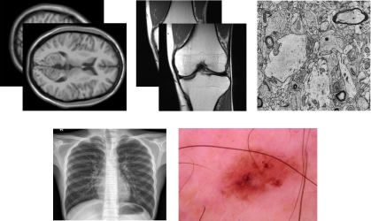
Figure 4: A sample of each dataset used for evaluation in this study. From top to bottom and left to right: 3D Brain MRI [6], 3D knee MRI [53], EM [49], chest X-ray [18], and dermatoscopic RGB [46].

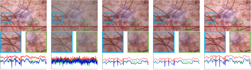
(a) HAM10000 Dermatoscopic RGB

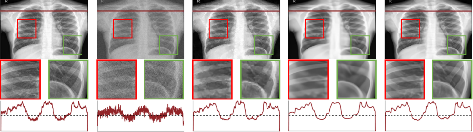
(b) Chest X-Ray

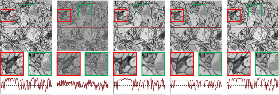
(c) EM

Figure 5: Color and gray-scale image denoising results on a) skin, b) chest, and c) EM images with noise level 35. From left to right: Reference, noisy, BM3D, SwinIR, and the proposed ADL.

For 2D databases, we compared the proposed ADL to improved BM3D [29] as the conventional model-based method, and three deep learning-based methods, Dynamic Residual Attention Network (DRAN) [40], DnCNN-S [55], and recently-developed SwinIR [24]. We compared the 3D version of our model to BM4D [27] that is widely used for denoising 3D biomedical image data.

4.1 Experiments with 2D data with synthetic noise

Synthesised WGN with $\sigma\in[10,15,25,35,50]$ were added into the test images of the skin [46], chest [18], and EM [49] datasets. The PSNR (dB) and SSIM results for different methods are represented in Table 1. According to the PSNR and SSIM results, one can see that the deep learning techniques yield better results compared to the model-based BM3D. The results of ADL are on par with those of the other methods, and it outperforms the other competing methods by a large margin for almost any noise level. The standard deviation measures the compactness of the denosing results. Although our method was not trained on the training sets (see Section 4), its PSNR’s standard deviation are on par with the conventional techniques’ ones. The SSIM results report that ADL gained the most compact results over all the noise levels. Fig. 5 shows a denoising example of different methods on the 2D datasets with noise level 35. To save space, we only show the results of model-based BM3D and SwinIR as SwinIR was the best one among the competing deep learning-based techniques. The example images are accompanied by profile lines. In the HAM10000 dataset (see Fig. 5(a)), ADL could recover much sharper edges than BM3D and SwinIR while maintaining the contrast of the reference image. The RGB profile lines of ADL have the highest similarity with the reference ones while the competing methods failed to preserve the contrast.

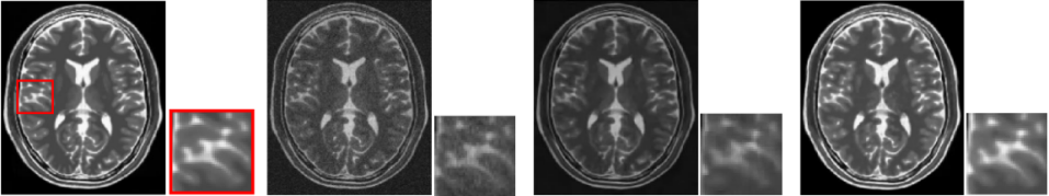
Figure 6: Denoising results of BM4D and the proposed ADL on the BrainWeb data with noise level 9 and RF 40%. From left to right: Reference, noisy, BM4D, and proposed ADL.

In the Chest X-Ray dataset (Fig. 5(b)), although the profile lines of all the methods were highly correlated to the reference one, ADL preserved more textural information compared to the others. BM3D resulted in blurred texture regions and SwinIR smoothed out the bones while the proposed ADL recovered more fine details and textures. The same trend is seen in the EM results depicted in Fig. 5(c), where SwinIR yielded a toy-like result and BM3D blurred the borders. The smoothness of BM3D and SwinIR is apparaent in their profile lines while the profile line of ADL tracked the reference one tightly. This means that ADL could successfully preserve the contrast and edges of the reference.

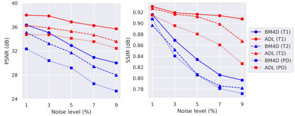
Figure 7: Average PSNR(dB) and SSIM of BM4D [27] and the proposed ADL on the BrainWeb database [6].

Table 2: PSNR (dB) and SSIM results (average $\pm$ standard deviation) of BM4D [27] and the proposed ADL on the 3D MRI knee dataset [53] for noise levels 10, 15, 25, 35, 50. The best results are highlighted in boldface.

Dataset	Noise Level	PSNR$\uparrow$		SSIM$\uparrow$
		BM4D	ADL	BM4D	ADL
		[27]	(ours)	[27]	(ours)
	10	37.1$\pm$1.8	38.3$\pm$1	0.89$\pm$0.04	0.92$\pm$0.02
	15	35.9$\pm$1.6	36.9$\pm$1.1	0.87$\pm$0.05	0.90$\pm$0.03
fastMRI [53]	25	34.3$\pm$1.4	35.1$\pm$1.1	0.85$\pm$0.05	0.89$\pm$0.03
	35	33.1$\pm$1.2	34.1$\pm$1	0.82$\pm$0.04	0.88$\pm$0.03
	50	31.5$\pm$1.1	33.1$\pm$0.9	0.78$\pm$0.04	0.86$\pm$0.04

4.2 Experiments with 3D data with synthetic noise

Similarly to the 2D experiment, synthesised WGN with $\sigma\in[10,15,25,35,50]$ were added into the test images in the fastMRI [53] dataset. The quantitative results are tabulated in Table 2. The noise in the simulated BrainWeb images has Rayleigh statistics in the background and Rician statistics in the signal regions. The average PSNR (dB) and SSIM results of the BM4D and the proposed ADL on the BrainWeb database are plotted in Fig. 7. ADL was able to reduce the noise effects to a greater extent as compared to BM4D. The results of both the databases verify the high performance of ADL in noise and RF distortion removal. Fig. 6 provides a comparison of the visual results of BM4D and ADL on a noisy T2-weighted image of BrainWab with noise level of 9 and RF 40%. From the appearance perspective, ADL preserved the histogram better than BM4D. Since the edges are blur in the BM4D result, in particular the zoom region, ADL restored the texture successfully. In short, the results of 3D are in consonance with 2D results and ADL well restored both the appearance and texture information.

4.3 Experiments with noisy data with no reference

We experimented the denoising with a T1-weighted brain MRI from OASIS3-project [21], selected randomly (male, cognitively normal, 87 years), and with a high-resolution EM dataset from rats’ corpus callosum [1]. The input noisy images, the denoised results by ADL, and the histogram of images are depicted in Fig. 8(b). Both the denoised results and the histogram plots verify that ADL successfully denoised the noisy images and preserved structural information with high precision.

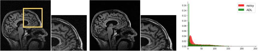
(a) Brain MRI

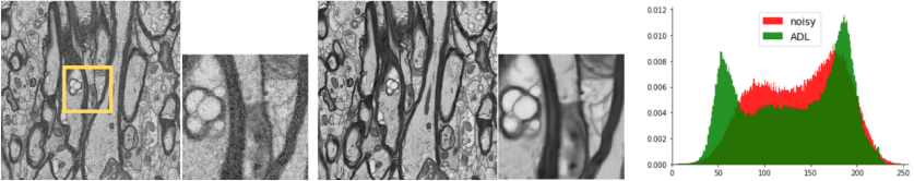
(b) EM

Figure 8: ADL results on no-reference noisy images. From left to right: noisy, ADL, and histograms of the input noisy and the denoised image.

4.4 Computational complexity

Table 3 reports the running time of the methods. The size of data for 2D and 3D experiments is $256\times 256$ and $256\times 256\times 256$, respectively. For 2D data, our denoiser needs less than 5 $M$ parameters which is much lower than 11.9$M$ of SwinIR. ADL also needs 2$G$ FLOPs which is considerably lower than that of SwinIR. For this reason, we named the proposed Unet as Efficient-Unet. For 3D data, Our denoiser does not require the cumbersome calculation of BM4D and this characteristic of our method is more appealing for real-time applications.

Table 3: Computational complexity and running time of different methods over 256$\times$256 2D and 256$\times$256$\times$256 3D MRI data.

	Method	Model Parameters	FLOPs	Running Time
		($M$)	($G$)
2D	SwinIR [24]	11.9	71.2	539 $ms$
	ADL (ours)	4.75	2.1	143 $ms$
3D	BM4D [27]	-	-	597.6 $s$
	ADL (ours)	14.8	121	14.6 $s$

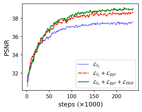
Figure 9: PSNR (dB) results of ADL for the validation using different loss functions. The results are averaged over noise levels 10, 15, 25, 35, and 50.

4.5 Ablation study

Multiscale loss functions: Fig. 9 compares the performance of ADL for different loss functions. The average PSNR results on the validation dataset when $\sigma\in[10,50]$ is reported here. It is seen that the pyramidal loss function considerably enhanced PSNR. This scheme was further improved by adding the histogram loss into the training.

Content Enhancer block: As described in Section 3.1, this block contributes to the denoising process directly when the depth of noise is low. In other words, the aim of the Content Enhancer block is to alleviate the vanishing-gradient problem in DNNs when the input noise is low, so it improves the convergence pace. We plotted the response of a few filters in the Content Enhancer block in Fig. 10. We also reported the correlation between the filer responses and the denoised images by ADL. It is worth noting that the filter responses for edges and texture are not reported here because it is not straightforward to measure the texture similarity between the edge-oriented filters and the denoised contents. For noise levels less than 10, one can observe that filters’ responses are highly correlated to the denoised contents and this scheme is reduced by increasing the level of AWGN noise. It can be referred from the results that the filters of the Content Enhancer block are highly contributed to the denoised content when the level of noise is small. Since the ADL outcomes remained almost unchanged over high-level noise, we deduce that the network switched to the decoders’ filters in this condition.

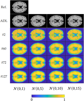
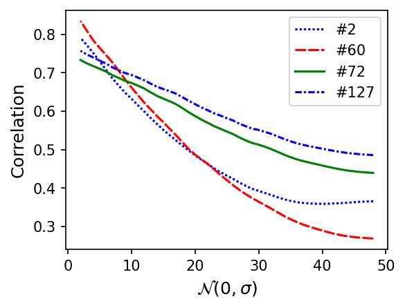
Figure 10: Performance of the Content Enhancer block in the Efficient-Unet for different noise levels. Top: Visual comparison of the response of few filters. Bottom: The correlation between the response of the filters and the ADL outcome.

5 Conclusion

In this study, we have proposed a novel adversarial distortion learning technique, named ADL, for efficiently restoring images from noisy and distorted observations. The key idea is to design an auto-encoder called Efficient-Unet that preserves texture and appearance during distortion removal. Efficient-Unet is based on a hierarchical approach in which low-level features are highly dependent on high-level ones. This enforces the model to restore the images from coarse to fine scales. To alleviate the vanishing-gradient problem and to improve the convergence pace, we added the Content Enhancer block to Efficient-Unet. The proposed model has been implemented for both 2D and 3D image data. For training the ADL’s parameters, we have proposed a pyramidal loss function for preserving textural information in different scales. We have also introduced a histogram loss to keep the appearance of the denoised contents. Experimental results and a comparative study with the conventional techniques over several publicly accessible 2D and 3D datasets have shown that ADL can restore more accurate images in the shortest time, which makes it more suitable for real-time applications.

Acknowledgment

We acknowledge the HPC resources by Bioinformatics Center, University of Eastern Finland. Data were provided in part by OASIS-3: PIs: T. Benzinger, D. Marcus, J. Morris; NIH P50 AG00561, P30 NS09857781, P01 AG026276, P01 AG003991, R01 AG043434, UL1 TR000448, R01 EB009352.

References

- [1] A Abdollahzadeh, I Belevich, et al. Deepacson automated segmentation of white matter in 3d electron microscopy. Communications biology, 4(1):1–14, 2021.
- [2] S Bera and P Biswas. Noise conscious training of non local neural network powered by self attentive spectral normalized markovian patch gan for low dose ct denoising. IEEE Trans. Med. Imaging, 40(12):3663–3673, 2021.
- [3] J Cai, X Jia, et al. Cine cone beam ct reconstruction using low-rank matrix factorization: algorithm and a proof-of-principle study. IEEE Trans. Med. Imaging, 33(8):1581–1591, 2014.
- [4] Stanley H Chan, R Khoshabeh, et al. An augmented lagrangian method for total variation video restoration. IEEE Trans. Image Process., 20(11):3097–3111, 2011.
- [5] G Chen, B Dong, et al. Denoising of diffusion mri data via graph framelet matching in xq space. IEEE Trans. Med. Imaging, 38(12):2838–2848, 2019.
- [6] C Cocosco, V Kollokian, et al. Brainweb: Online interface to a 3d mri simulated brain database. In NeuroImage. Citeseer, 1997. The dataset is available at https://brainweb.bic.mni.mcgill.ca/.
- [7] K Dabov, A Foi, et al. Image denoising by sparse 3-d transform-domain collaborative filtering. IEEE Trans. Image Process., 16(8):2080–2095, 2007.
- [8] M Elad and M Aharon. Image denoising via sparse and redundant representations over learned dictionaries. IEEE Trans. Image Process., 15(12):3736–3745, 2006.
- [9] Y Gal, JH Mehnert, et al. Denoising of dynamic contrast-enhanced mr images using dynamic nonlocal means. IEEE Trans. Med. Imaging, 29(2):302–310, 2009.
- [10] P Getreuer. Rudin-osher-fatemi total variation denoising using split bregman. Image Processing On Line, 2:74–95, 2012.
- [11] M Ghahremani, Y Liu, and B Tiddeman. Ffd: Fast feature detector. IEEE Trans. Image Process., 30:1153–1168, 2020.
- [12] L Gondara. Medical image denoising using convolutional denoising autoencoders. In IEEE international conference on data mining workshops (ICDMW), pages 241–246. IEEE, 2016.
- [13] I Goodfellow, J Pouget-Abadie, et al. Generative adversarial nets. Advances in neural information processing systems, 27, 2014.
- [14] Onur G Guleryuz. Weighted averaging for denoising with overcomplete dictionaries. IEEE Trans. Image Process., 16(12):3020–3034, 2007.
- [15] K He, X Zhang, et al. Deep residual learning for image recognition. In CVPR, pages 770–778, 2016.
- [16] Y Huang, W Xia, et al. Noise-powered disentangled representation for unsupervised speckle reduction of optical coherence tomography images. IEEE Trans. Med. Imaging, 40(10):2600–2614, 2020.
- [17] P Kaur, G Singh, and P Kaur. A review of denoising medical images using machine learning approaches. Current medical imaging, 14(5):675–685, 2018.
- [18] D Kermany, M Goldbaum, et al. Identifying medical diagnoses and treatable diseases by image-based deep learning. Cell, 172(5):1122–1131, 2018. The dataset is available at https://www.kaggle.com/datasets/paultimothymooney/chest-xray-pneumonia.
- [19] D Kingma and J Ba. Adam: A method for stochastic optimization. arXiv preprint arXiv:1412.6980, 2014.
- [20] Z Kong, L Han, X Liu, and X Yang. A new 4-d nonlocal transform-domain filter for 3-d magnetic resonance images denoising. IEEE Trans. Med. Imaging, 37(4):941–954, 2017.
- [21] J. LaMontagne, LS. Benzinger, et al. Oasis-3: Longitudinal neuroimaging, clinical, and cognitive dataset for normal aging and alzheimer disease. medRxiv, 2019.
- [22] K Lee and W Jeong. Iscl: Interdependent self-cooperative learning for unpaired image denoising. IEEE Trans. Med. Imaging, 40(11):3238–3248, 2021.
- [23] K Li, W Zhou, et al. Assessing the impact of deep neural network-based image denoising on binary signal detection tasks. IEEE Trans. Med. Imaging, 40(9):2295–2305, 2021.
- [24] J Liang, J Cao, et al. Swinir: Image restoration using swin transformer. In ICCV, pages 1833–1844, 2021.
- [25] J Liu, Y Pan, et al. Applications of deep learning to mri images: A survey. Big Data Mining and Analytics, 1(1):1–18, 2018.
- [26] Y Ma, Y Liu, et al. Cycle structure and illumination constrained gan for medical image enhancement. In International conference on medical image computing and computer-assisted intervention, pages 667–677. Springer, 2020.
- [27] M Maggioni, V Katkovnik, et al. Nonlocal transform-domain filter for volumetric data denoising and reconstruction. IEEE Trans. Image Process., 22(1):119–133, 2012.
- [28] J Mairal, F Bach, et al. Non-local sparse models for image restoration. In ICCV, pages 2272–2279. IEEE, 2009.
- [29] Y Mäkinen, L Azzari, and A Foi. Collaborative filtering of correlated noise: Exact transform-domain variance for improved shrinkage and patch matching. IEEE Trans. Image Process., 29:8339–8354, 2020.
- [30] V Manjón, P Coupé, et al. Adaptive non-local means denoising of mr images with spatially varying noise levels. Journal of Magnetic Resonance Imaging, 31(1):192–203, 2010.
- [31] Mehdi Mirza and Simon Osindero. Conditional generative adversarial nets. arXiv preprint arXiv:1411.1784, 2014.
- [32] S Mohan, Z Kadkhodaie, et al. Robust and interpretable blind image denoising via bias-free convolutional neural networks. arXiv preprint arXiv:1906.05478, 2019.
- [33] K Papafitsoros and C Schönlieb. A combined first and second order variational approach for image reconstruction. Journal of mathematical imaging and vision, 48(2):308–338, 2014.
- [34] V Papyan, Y Romano, et al. Convolutional dictionary learning via local processing. In ICCV, pages 5296–5304, 2017.
- [35] M Quan, D Hildebrand, et al. Removing imaging artifacts in electron microscopy using an asymmetrically cyclic adversarial network without paired training data. In ICCV, pages 3804–3813. IEEE, 2019.
- [36] S Rai, S Bhatt, and S Patra. An unsupervised deep learning framework for medical image denoising. arXiv preprint arXiv:2103.06575, 2021.
- [37] O Russakovsky, J Deng, et al. Imagenet large scale visual recognition challenge. Int. J. Comput. Vis., 115(3):211–252, 2015.
- [38] V Sagheer and N George. A review on medical image denoising algorithms. Biomedical signal processing and control, 61:102036, 2020.
- [39] E Schonfeld, B Schiele, and A Khoreva. A u-net based discriminator for generative adversarial networks. In CVPR, pages 8207–8216, 2020.
- [40] S Sharif, R Naqvi, and M Biswas. Learning medical image denoising with deep dynamic residual attention network. Mathematics, 8(12):2192, 2020.
- [41] Y Sidky and X Pan. Image reconstruction in circular cone-beam computed tomography by constrained, total-variation minimization. Physics in Medicine & Biology, 53(17):4777, 2008.
- [42] J Starck, J Fadili, and F Murtagh. The undecimated wavelet decomposition and its reconstruction. IEEE Trans. Image Process., 16(2):297–309, 2007.
- [43] B Stimpel, C Syben, et al. Multi-modal deep guided filtering for comprehensible medical image processing. IEEE Trans. Med. Imaging, 39(5):1703–1711, 2019.
- [44] H Talebi, M Delbracio, and P Milanfar. Projected distribution loss for image enhancement. 2021.
- [45] B Tiddeman and M Ghahremani. Principal component wavelet networks for solving linear inverse problems. Symmetry, 13(6):1083, 2021.
- [46] Philipp Tschandl. The HAM10000 dataset, a large collection of multi-source dermatoscopic images of common pigmented skin lesions, 2018.
- [47] TensorFlow: ReduceLROnPlateau — TensorFlow Core v2.8.0 documentation. https://www.tensorflow.org/api_docs/python/tf/keras/callbacks/ReduceLROnPlateau.
- [48] W Wang, F Li, and K Ng. Structural similarity-based nonlocal variational models for image restoration. IEEE Trans. Im. Proc., 28(9):4260–4272, 2019.
- [49] D Wei, Z Lin, et al. Mitoem dataset: Large-scale 3d mitochondria instance segmentation from em images. In International Conference on Medical Image Computing and Computer Assisted Intervention, 2020. The dataset is available at https://mitoem.grand-challenge.org/.
- [50] D Wu, H Ren, and Q Li. Self-supervised dynamic ct perfusion image denoising with deep neural networks. IEEE Transactions on Radiation and Plasma Medical Sciences, 5(3):350–361, 2020.
- [51] Q Xu, H Yu, et al. Low-dose x-ray ct reconstruction via dictionary learning. IEEE Trans. Med. Imaging, 31(9):1682–1697, 2012.
- [52] Q Yang, P Yan, et al. Low-dose ct image denoising using a generative adversarial network with wasserstein distance and perceptual loss. IEEE Trans. Med. Imaging, 37(6):1348–1357, 2018.
- [53] J Zbontar, F Knoll, et al. fastmri: An open dataset and benchmarks for accelerated mri. arXiv preprint arXiv:1811.08839, 2018. The dataset is available at https://fastmri.org/dataset/.
- [54] K Zhang, Y Li, et al. Plug-and-play image restoration with deep denoiser prior. IEEE Trans. Pattern Anal. Mach. Intell., 2021.
- [55] K Zhang, W Zuo, et al. Beyond a gaussian denoiser: Residual learning of deep cnn for image denoising. IEEE Trans. Image Process., 26(7):3142–3155, 2017.
- [56] Y Zhang, Y Wang, et al. Statistical iterative reconstruction using adaptive fractional order regularization. Biomedical optics express, 7(3):1015–1029, 2016.
- [57] J Zhu, T Park, et al. Unpaired image-to-image translation using cycle-consistent adversarial networks. In ICCV, pages 2223–2232, 2017.
- [58] W Zuo, L Zhang, et al. Texture enhanced image denoising via gradient histogram preservation. In CVPR, pages 1203–1210, 2013.