Recovery by discretization corrected
particle strength exchange (DC PSE) operators

Abstract

A new recovery technique based on discretization corrected particle strength exchange (DC PSE) operators is developed in this paper. DC PSE is a collocation method that can be used to compute derivatives directly at nodal points, instead of by projection from Gauss points as is done in many finite element-based recovery techniques. The proposed method is truly meshless and does not require patches of elements to be defined, which makes it generally applicable to point clouds and arbitrary element topologies. Numerical examples show that the proposed method is accurate and robust.

1 Introduction

In computational science and engineering there are many problems in which the gradient of the solution, rather than the solution itself, is of primary interest. Examples include strain and stress in structural analysis and wall shear stress in fluid dynamics. The goal of this paper is to develop a meshfree method for the accurate and robust recovery of gradients, and other derived quantities such as strain and stress, from discrete scalar or vector fields with values defined at nodal points. These nodal values are typically obtained numerically, using for example the finite element (FE) method. However, the nodal values may also be obtained analytically or from measurements, an example of the latter being the computation of strain from image data (Choi et al., 1991; López-Linares et al., 2019).

The finite element method (FEM) has become the dominant method for solving partial differential equations (PDEs) in problems with complex geometries. However, the calculation of accurate stresses in the displacement-based FE method is a notoriously difficult problem (Oden and Brauchli, 1971). In the FE method, the function (e.g. displacement) is best sampled at the nodal points but the best accuracy for the gradient (and derived quantities such as strain and stress) is obtained at the superconvergent Gauss points corresponding to the order of polynomial used for the solution (Zienkiewicz and Zhu, 1995; Zienkiewicz et al., 2013). Recovery methods are often used to smooth the discontinuous derivatives and derived quantities (strain and stress) resulting from piecewise continuous approximations of the solution variables in finite element computations (Zienkiewicz et al., 2013). Numerous recovery methods have been proposed to obtain continuous gradient, strain and stress fields from the discontinuous fields obtained using FEM (Oden and Brauchli, 1971; Kelly et al., 1983; Zienkiewicz and Zhu, 1987; Zienkiewicz and Zhu, 1992; Boroomand and Zienkiewicz, 1997; Zhang and Naga, 2005). An important application of recovery methods is their use in a posteriori error estimators that are based on measuring the difference between the direct and post-processed approximations to the gradient (Zienkiewicz and Zhu, 1987; Ainsworth and Oden, 2000).

Meshless and meshfree methods (Chen and Belytschko, 2015; Fasshauer, 2007) have been proposed as an alternative to global and local recovery methods based on finite elements. Compared with finite element based methods which often require patches of neighboring elements to be defined, meshfree methods do not rely on element connectivity and can therefore be applied easily to almost arbitrary point clouds (some limitations on the distribution of points remain based on invertibility of matrices and conditioning of linear systems that must be solved to construct the shape functions). The problem is typically posed as an approximation or curve fitting problem whereby the values are known at one set of points (typically the quadrature points) and these are to be interpolated as accurately as possible to a different set of points (typically the nodal points). This approach can also be applied to the recovery of stress in meshfree solution methods such as the element-free Galerkin method (Lee and Zhou, 2004). Ahmed et al. (2018) showed that a meshfree approach based on moving least squares approximation can be used to improve the performance of error recovery techniques as compared to the superconvergent patch recovery (SPR) method (Zienkiewicz and Zhu, 1992). Ahmed (2020) compared the element-free Galerkin and radial point interpolation methods that use the moving least squares (MLS) interpolation (radial weighting function) and the radial point interpolation (polynomial and radial basis function), respectively, against the mesh-dependent least squares interpolation error recovery (SPR) (Zienkiewicz and Zhu, 1992) and found that the quality of meshless and mesh-based RPIM and MLS based error estimation is superior to mesh-dependent SPR.

In this paper, rather than evaluating the gradient, strain or stress at the integration points and interpolating these values to the nodal points, we aim to compute the gradient, strain and stress directly at the nodal points given the nodal data. To this end, we develop an accurate, efficient and generally applicable meshfree approach for recovery of gradients given the solution at nodal points based on discretization corrected particle strength exchange (DC PSE) operators (Schrader et al., 2010). DC PSE uses Taylor expansions on irregularly distributed point clouds to compute derivatives. We compute the derivatives of the unknown field function as a postprocessing procedure after its solution has been obtained and use these derivatives to compute derived quantities such as strain and stress.

The remainder of the paper is organized as follows. In section 2, we state the governing equations of linear elasticity and describe their solution using the FEM. We then present the DC PSE operators as an alternative to the FEM for computing derivatives at nodal points, and explain how we apply DC PSE as a post-processing tool to obtain strain and stress from a given displacement field. In section 3, we demonstrate the accuracy of the proposed recovery method by applying it to several benchmark problems, as well as a more realistic practical example involving the calculation of stress within the wall of an abdominal aortic aneurysm (AAA). Finally, in section 4 we discuss the pros and cons of the proposed approach and make some suggestions for further research in this area.

2 Methods

2.1 Governing equations of linearized elasticity

In this study, we consider elliptic PDEs of the following form. Consider the region $\Omega\subset\mathbb{R}^{d}$, where $d=1,2$ (plane strain) or $3$. The boundary $\partial\Omega$ of the domain is decomposed into two disjoint parts such that $\overline{\Gamma_{D}\cup\Gamma_{N}}=\partial\Omega$ and $\Gamma_{D}\cap\Gamma_{N}=\emptyset$. The unit outward normal vector on $\partial\Omega$ is denoted by $\bm{n}$. Known displacements and tractions, $\bm{u}_{D}$ and $\bm{g}$, are prescribed on $\Gamma_{D}$ and $\Gamma_{N}$, respectively. Body forces $\bm{f}$ are prescribed in $\Omega$. The strong form of the boundary value problem of elastostatics can then be written as follows. Given $\bm{f}:\Omega\to\mathbb{R}^{d}$, $\bm{g}:\Gamma_{N}\to\mathbb{R}^{d}$ and $\bm{u}_{D}:\Gamma_{D}\to\mathbb{R}^{d}$; find $\bm{u}:\Omega\to\mathbb{R}^{d}$ such that

$$-\mathrm{div}\,\bm{\sigma}(\bm{u}) =\bm{f} \text{ in }\Omega,$$ (1)

$$\bm{\sigma}(\bm{u})\cdot\bm{n} =\bm{g} \text{ on }\Gamma_{N},$$ (2)

$$\bm{u} =\bm{u}_{D} \text{ on }\Gamma_{D}.$$ (3)

The constitutive equation for linear elastostatics is given by the generalized Hooke’s law

$$\bm{\sigma}(\bm{u})=2\mu\bm{\epsilon}(\bm{u})+\lambda\mathrm{tr}\bm{\epsilon}(\bm{u}),$$ (4)

where the linearized strain

$$\bm{\epsilon}=\frac{1}{2}\left(\nabla\bm{u}+\nabla\bm{u}^{T}\right),$$ (5)

is the symmetric part of the displacement gradient $\nabla\bm{u}$. The first and second Lamé parameters, $\lambda$ and $\mu$, are related to Young’s modulus and Poisson’s ratio, $E$ and $\nu$, by

$$\lambda=\frac{E\nu}{(1+\nu)(1-2\nu)}\quad\text{ and }\quad\mu=\frac{E}{2(1+\nu)}.$$ (6)

2.2 DC PSE derivative operators

Before describing their application to the proposed recovery method we first summarize the derivation and computation of the discretization corrected (DC) particle strength exchange (PSE) operators that we will use to compute derivatives (Reboux et al., 2012; Schrader et al., 2012). The DC PSE method is similar to operators used to approximate derivatives, such as the finite difference method, corrected smoothed-particle hydrodynamics (SPH) method, reproducing kernel particle method (RKPM) and moving least squares (MLS) (Schrader, 2011). Their main advantage is that, due to their meshless nature, they can be applied relatively easily to arbitrarily complex geometries. In this section, we provide a succinct summary of the method as background for the next section where we apply DC PSE to compute the displacement gradient. Further details on the derivation and numerical aspects of the DC PSE operators can be found in the earlier contributions (Schrader, 2011; Reboux et al., 2012; Schrader et al., 2012).

We define the DC PSE operator for approximating the spatial derivative $\bm{D}^{m,n}f(\bm{x})$ as:

$$\bm{Q}^{m,n}f(\bm{x}_{p})=\frac{1}{\epsilon(\bm{x}_{p})^{m+n}}\sum_{\bm{x}_{q}\in N(\bm{x}_{p})}\left(f(\bm{x}_{q})\pm f(\bm{x}_{p})\right)\frac{1}{\epsilon(\bm{x}_{p})^{2}}\eta\left(\frac{\bm{x}_{p}-\bm{x}_{q}}{\epsilon(\bm{x}_{p})}\right),$$ (7)

where $\epsilon(\bm{x})$ is a spatially dependent scaling or resolution function, $\eta(\bm{x},\epsilon(\bm{x}))$ is a kernel function normalized by the factor $\epsilon(\bm{x}_{p})^{-2}$, and $N(\bm{x}_{p})$ is the set of points in the support of the kernel function.

We construct the DC PSE operators such that when we decrease the average spacing between nodes, $h(\bm{x}_{p})\rightarrow 0$, the operator converges to the spatial derivative $\bm{D}^{m,n}f(\bm{x}_{p})$ with an asymptotic rate $r$:

$$\bm{Q}^{m,n}f(\bm{x}_{p})=\bm{D}^{m,n}f(\bm{x}_{p})+\mathcal{O}(h(\bm{x}_{p})^{r}),$$ (8)

where the component-wise average neighbor spacing is given as $h(\bm{x}_{p})=\frac{1}{N}\sum\limits_{\bm{x}_{q}\in N(\bm{x})}|(x-x_{q})|+|(y-y_{q})|$, where $N$ is the number of nodes in the support of $\bm{x}_{p}$. Therefore, we need to find a kernel function $\eta(\bm{x})$ and a scaling relation $\epsilon(\bm{x}_{p})$ as to satisfy Eq. (8). To achieve this, we replace the terms $f(\bm{x}_{q})$ in Eq. (7) with their Taylor series expansions around the point $\bm{x}_{p}$. This substitution gives:

$$\begin{split}\bm{Q}^{m,n}f(\bm{x}_{p})&=\frac{1}{\epsilon(\bm{x}_{p})^{m+n}}\sum_{\bm{x}_{q}\in N(\bm{x}_{p})}\Biggl{(}\sum_{i=0}^{\infty}\sum_{j=0}^{\infty}\frac{(x_{p}-x_{q})^{i}(y_{p}-y_{q})^{j}(-1)^{i+j}}{i!j!}\bm{D}^{i,j}f(\bm{x}_{p})\\ &\pm f(\bm{x}_{p})\Biggr{)}\frac{1}{\epsilon(\bm{x}_{p})^{2}}\eta\left(\frac{\bm{x}_{p}-\bm{x}_{q}}{\epsilon(\bm{x}_{p})}\right).\end{split}$$ (9)

It is convenient to re-write Eq. (9) in the form:

$$\begin{split}\bm{Q}^{m,n}f(\bm{x}_{p})&=\left(\sum_{i=0}^{\infty}\sum_{j=0}^{\infty}\frac{\epsilon(\bm{x}_{p})^{i+j-m-n}(-1)^{i+j}}{i!j!}\bm{D}^{i,j}f(\bm{x}_{p})Z^{i,j}(\bm{x}_{p})\right)\\ &\pm Z^{0,0}(\bm{x}_{p})\epsilon(\bm{x}_{p})^{-m-n}f(\bm{x}_{p}),\end{split}$$ (10)

where

$$Z^{i,j}(\bm{x}_{p})=\sum_{\bm{x}_{q}\in N(\bm{x}_{p})}\frac{(x_{p}-x_{q})^{i}(y_{p}-y_{q})^{j}(-1)^{i+j}}{\epsilon(\bm{x}_{p})^{i+j}}\frac{1}{\epsilon(\bm{x}_{p})^{2}}\eta\left(\frac{\bm{x}_{p}-\bm{x}_{q}}{\epsilon(\bm{x}_{p})}\right).$$ (11)

We call $Z^{i,j}(\bm{x}_{p})$ the discrete moments. Now, if we restrict the scaling parameter $\epsilon(\bm{x}_{p})$ to converge at the same rate as the average spacing between points $h(\bm{x}_{p})$, that is

$$\frac{h(\bm{x}_{p})}{\epsilon(\bm{x}_{p})}=\text{constant},$$ (12)

we find that the discrete moments $Z^{i,j}$ are $\mathcal{O}(1)$ as $h(\bm{x}_{p})\rightarrow 0$. Given Eq. (12), the convergence behavior of Eq. (8) is determined by the coefficients of the terms $\epsilon(\bm{x}_{p})^{i+j-m-n}\bm{D}^{i,j}$. We make the DC PSE operator satisfy Eq. (8) by ensuring the coefficients of the $(m,n)$ term is 1, and all other coefficients of $\epsilon(\bm{x}_{p})^{i+j-m-n}\bm{D}^{i,j}$ for $i+j-m-n<r$ are 0. This results in the following set of conditions for the discrete moments,

$$Z^{i,j}(\bm{x}_{p})=\begin{cases}i!j!(-1)^{i+j}&i=m,j=n,\\ 0&\alpha_{\text{min}}<i+j<r+m+n,\\ <\infty&\text{otherwise},\end{cases}$$ (13)

where $\alpha_{\text{min}}$ is 1 if $i+j$ is odd and 0 if even. This is due to the zeroth moment $Z^{0,0}$ canceling out for odd $i+j$. The choice of the factor $\epsilon(\bm{x}_{p})^{-m-n}$ in Eq. (7) simply acts as to simplify the expression of the moment conditions.

For the kernel function $\eta(\bm{x})$ to satisfy the $l$ conditions given in Eq. (13) for arbitrary neighborhood node distributions, the operator must have $l$ degrees of freedom. This leads to the requirement that the support $N(\bm{x})$ of the kernel function has to include at least $l$ nodes. In this paper we use kernel functions for the operator of the form

$$\eta(\bm{x})=\begin{cases}\sum\limits_{i,j}^{i+j<r+m+n}a_{i,j}x^{i}y^{i}=je^{-x^{2}-y^{2}}&\sqrt{x^{2}+y^{2}}<r_{c},\\ 0&\text{otherwise.}\end{cases}$$ (14)

This is a monomial basis multiplied by an exponential window function, where $r_{c}$ sets the kernel support and the $a_{i,j}$ are scalars to be determined to satisfy the moment conditions in Eq. (13). The cut-off radius $r_{c}$ should be set to include at least $l$ collocation nodes in the support $N(x)$. To construct the operator $\bm{Q}^{m,n}f(\bm{x}_{p})$ at node $\bm{x}_{p}$, the coefficients are found by solving a linear system of equations from Eqs. (14) and (13). With our choice of kernel function we have,

$$\bm{Q}^{m,n}f(\bm{x}_{p})=\frac{1}{\epsilon(\bm{x}_{p})^{m+n}}\sum_{\bm{x}_{q}\in N(\bm{x}_{p})}\left(f(\bm{x}_{q})\pm f(\bm{x}_{p})\right)\bm{p}\left(\frac{\bm{x}_{q}-\bm{x}_{p}}{\epsilon(\bm{x}_{p})}\right)\bm{a}^{T}(\bm{x}_{p})e^{\frac{-(x_{p}-x_{q})^{2}-(y_{p}-y_{q})^{2}}{\epsilon(\bm{x}_{p})}},$$ (15)

where $\bm{p}(\bm{x})=\{p_{1}(x),p_{2}(x),\dots,p_{l}(x)\}$ and $\bm{a}(\bm{x})$ are vectors of the terms in the monomial basis and of their coefficients in Eq. (14), respectively. The normalization factor $\epsilon(\bm{x}_{p})^{-2}$ is absent, since it cancels out through the coefficients $\bm{a}(\bm{x}_{p})$. Using this formulation, the operator system becomes eassy to obtain.

The linear system for the kernel coefficients then is:

$$\bm{A}(\bm{x}_{p})\bm{a}^{T}(\bm{x}_{p})=\bm{b},$$ (16)

where

$$\bm{A}(\bm{x}_{p}) =\bm{B}(\bm{x}_{p})^{T}\bm{B}(\bm{x}_{p})\in\mathbb{R}^{l\times l}$$ (17)

$$\bm{B}(\bm{x}_{p})) =\bm{E}(\bm{x}_{p})^{T}\bm{V}(\bm{x}_{p})\in\mathbb{R}^{k\times l}$$ (18)

$$\bm{b} =(-1)^{m+n}\bm{D}^{m,n}\bm{p}(\bm{x})|_{x=0}\in\mathbb{R}^{l\times 1}.$$ (19)

The scalar $k>l$ is the number of nodes in the support of the operator, $l$ the number of moment conditions to be satisfied, and $\bm{V}(\bm{x}_{p})$ the Vandermonde matrix constructed from the monomial basis $\bm{p}(\bm{x}_{p})$. The diagonal matrix $\bm{E}(\bm{x}_{p})$ contains the square roots of the values of the exponential window function at the neighboring nodes in the operator support. Further, we define $\{\bm{z}_{i}\}_{i=1}^{k}=\{\bm{x}_{p}-\bm{x}_{q}\}_{\bm{x}_{q}\in N(\bm{x}_{p})}$, the set of vectors pointing from all neighboring nodes in the support of $\bm{x}_{p}$ to $\bm{x}_{q}$. So then explicitly

$$\bm{V}(\bm{x}_{p}) =\begin{pmatrix}p_{1}(\frac{\bm{z}_{1}}{\epsilon(\bm{x})})&p_{2}(\frac{\bm{z}_{1}}{\epsilon(\bm{x})})&\cdots&p_{l}(\frac{\bm{z}_{1}}{\epsilon(\bm{x})})\\ p_{1}(\frac{\bm{z}_{2}}{\epsilon(\bm{x})})&p_{2}(\frac{\bm{z}_{2}}{\epsilon(\bm{x})})&\cdots&p_{l}(\frac{\bm{z}_{2}}{\epsilon(\bm{x})})\\ \vdots&\vdots&\ddots&\vdots\\ p_{1}(\frac{\bm{z}_{k}}{\epsilon(\bm{x})})&p_{2}(\frac{\bm{z}_{k}}{\epsilon(\bm{x})})&\cdots&p_{l}(\frac{\bm{z}_{k}}{\epsilon(\bm{x})})\end{pmatrix}\in\mathbb{R}^{k\times l}$$ (20)

$$\bm{E}(\bm{x}_{p}) =\text{diag}\left(\left\{e^{\frac{-|\bm{z}_{i}|^{2}}{2\epsilon(\bm{x})}}\right\}_{i=1}^{k}\right)\in\mathbb{R}^{k\times k}.$$ (21)

Once the matrix $\bm{A}$ is constructed at each node $\bm{x}_{p}$, the linear systems can be solved for the coefficients $\bm{a}$ used in the DC PSE operators at each node as in Eq. (15). The matrix $\bm{A}$ only depends on the number of moment conditions $l$ and the local distribution of nodes in the support domain. The invertibility of $\bm{A}$ depends entirely on that of the Vandermonde matrix $\bm{V}$, due to $\bm{E}$ being a diagonal matrix with non-zero entries.

2.3 Recovery by DC PSE

The problem of recovering the gradient (and derived quantities such as stress and strain) can be considered as a typical curve/surface fitting problem where a function is sampled at a discrete number of points and we seek to determine the functions derivative at those points. The stress can be considered as a derived quantity, by which we mean that it is not a primary solution variable that must be computed to obtain a solution in displacements, but can be computed during post-processing of the results after the displacement is known.

After the displacement solution has been computed using the finite element method (or other suitable numerical method, or from experimental measurements) the displacement field is known at the nodal points of the discretized spatial domain. However, we are interested in the stress field, which is related to the strain. The strain is related to the gradient of the displacement. Hence, we require an accurate method for computing derivatives at specified points, given the value of the function at those points. The DC PSE operators are ideally suited to this task.

Once the displacement gradient $\nabla\bm{u}$ has been computed (using the displacement field and the DC PSE spatial derivatives defined in Eq. (15)), the strain and stress can be obtained by substitution of $\nabla\bm{u}$ into the constitutive equation (4). Other derived quantities such as principal stresses and stress invariants can be easily computed. For example, the von Mises stress is defined as

$$\sigma_{\mathrm{Mises}}=\sqrt{\frac{3}{2}\bm{s}:\bm{s}},$$ (22)

where $s$ is the deviatoric stress tensor

$$\bm{s}(\bm{u})=\bm{\sigma}(\bm{u})-\frac{1}{3}\mathrm{tr}\,\bm{\sigma}(\bm{u})\bm{I}.$$ (23)

We note briefly that this procedure applies only to path-independent materials because only the final displacement is used to compute the stress. For path-dependent materials, such as those exhibiting plastic behavior, a more elaborate procedure may be conceived whereby the stress is computed at each time increment using the current displacements and state-variables stored at the nodes (the state variables are typically stored only at the integration points because that is where stress is usually computed).

The salient advantage of the method described in this section is that all the derived quantities can be obtained from the known displacement field (obtained in the current study either analytically or using the finite element method) and the constitutive equation. This makes it straightforward to implement the proposed method as a post-processing tool in existing software irrespective of the methods used to solve the equations.

2.4 Quantitative measures of accuracy

DC PSE was originally developed as a collocation method, and, unlike the finite element method, the function values and gradients are defined at the nodes only. Similarly to finite difference methods, we do not use shape functions to compute function values at arbitrary locations within the domain so the integral error measures typically used for assessing the solution accuracy of FEM are not applicable. Instead, we use discrete error measures, namely the maximum absolute ($\infty$-norm) error and the normalized root mean square error (NRMSE) that are typically used for assessing the accuracy of collocation methods to compare the predictions of the proposed method with analytical and finite element solutions. The NRMSE between the estimated nodal values $\hat{\bm{y}}$ and the reference nodal values $\bm{y}$ is defined as

$$\mathrm{NRMSE}(\bm{y},\hat{\bm{y}})=\frac{\sqrt{\mathrm{MSE}(\bm{y},\hat{\bm{y}})}}{\bm{y}_{\mathrm{max}}-\bm{y}_{\mathrm{min}}},\quad\mathrm{MSE}(\bm{y},\hat{\bm{y}})=\frac{1}{n}\sum_{i=1}^{n}(\bm{y}_{i}-\hat{\bm{y}}_{i})^{2},$$ (24)

where $n$ is the total number of nodes. The maximum absolute ($\infty$-norm) error is defined as

$$||\bm{y}-\hat{\bm{y}}||_{\infty}=\mathrm{max}_{1\leq i\leq n}|\bm{y}_{i}-\hat{\bm{y}}_{i}|.$$ (25)

3 Results

In this section, we demonstrate the accuracy of our proposed meshfree recovery method for some benchmark problems that have analytical solutions, before applying the method to a practical example of computing stress within the wall of an abdominal aortic aneurysm (AAA). We compare the proposed meshfree DC PSE method with the following commonly used finite elements: triangles and tetrahedra with linear (P1) and quadratic (P2) Lagrange bases; and quadrilaterals and hexahedra with linear (Q1) and quadratic (Q2) tensor-product Lagrange bases.

3.1 Franke’s function

The following function, introduced by Franke (1979), is commonly used to evaluate the performance of meshfree methods. It consists of two Gaussian peaks and a sharper Gaussian dip superimposed on a surface sloping towards the first quadrant, and is defined as

$$u(x,y)=0.75\,\mathrm{exp}\left[-\frac{(9x-2)^{2}+(9y-2)^{2}}{4}\right]+0.75\,\mathrm{exp}\left[-\frac{(9x+1)^{2}}{49}+\frac{(9y+1)^{2}}{10}\right]\\ +0.5\,\mathrm{exp}\left[-\frac{(9x-7)^{2}+(9y-3)^{2})}{4}\right]-0.2\,\mathrm{exp}\left[-(9x-4)^{2}+(9y-7)^{2}\right].$$ (26)

Given the solution (26), we computed the derivatives numerically at the nodal points using the FE and DC PSE methods to compare the accuracy of the recovered gradients $\mathrm{\partial}u/\mathrm{\partial}x$ and $\mathrm{\partial}u/\mathrm{\partial}y$ against the analytical derivatives. We used structured quadrilateral and triangular meshes, as well as unstructured triangular meshes, to discretize the spatial domain; and used the same meshes for the FE and DC PSE methods (disregarding the nodal connectivity when using DC PSE). For the FE method, we used linear (P1) and quadratic (P2) triangular, and linear (Q1) and quadratic (Q2) quadrilateral finite elements.

Fig. 1 shows representative quadrilateral and triangle meshes used for this problem. The nodal distribution corresponding to the quadrilateral elements for a given Q2 mesh and a refined Q1 mesh obtained by splitting the elements of the Q1 mesh are equivalent, with both meshes having the same number of nodes, node spacing $h$ and nodal coordinates (only the number of elements and element nodal connectivity is different). Hence, the DC PSE derivatives for these two grids will be equivalent when the function values at the nodes are the same. The triangular P1 and P2 meshes share similar similarities.

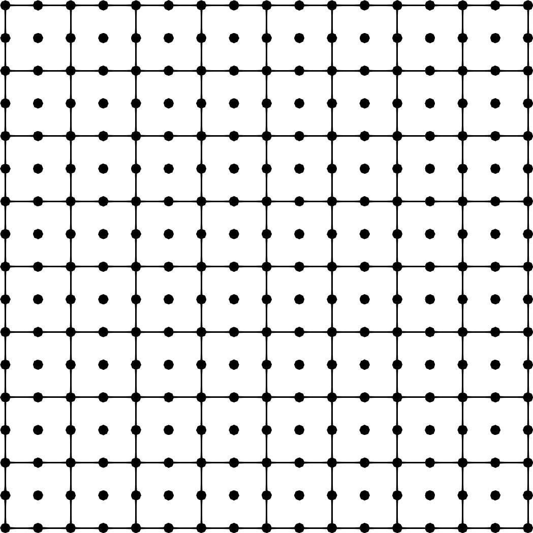
(a)

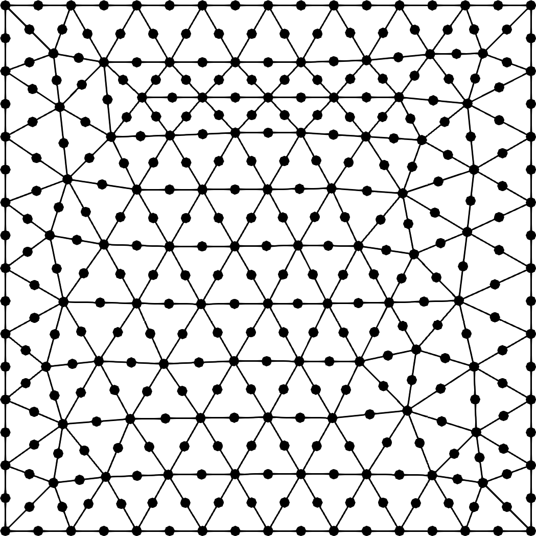
(b)

Figure 1: The (a) coarsest structured quadratic quadrilateral (Q2) and (b) coarsest unstructured quadratic triangle (P2) meshes used for Franke’s function benchmark problem. The meshes have (a) 289 nodes ($h=0.063$) and 64 elements, and (b) 357 nodes ($h=0.056$) and 162 elements, respectively. The coarsest linear quadrilateral and triangle meshes have a similar number of nodes with more elements.

Fig. 2 shows the convergence of the normalized root mean square error (NRMSE) and the maximum absolute ($\infty$-norm) error in the derivatives $\mathrm{\partial}u/\mathrm{\partial}x$ and $\mathrm{\partial}u/\mathrm{\partial}y$ of Franke’s function computed using the FE and DC PSE methods. As expected, the derivatives computed using quadratic (P2 and Q2) finite elements and DC PSE converge more rapidly, and are significantly more accurate, than those computed using linear (P1 and Q1) finite elements. Moreover, the DC PSE derivatives are slightly more accurate and converge slightly faster than the quadratic finite elements for both the quadrilateral and triangle meshes. These results suggest that DC PSE is well suited for accurately recovering the gradients of a given function.

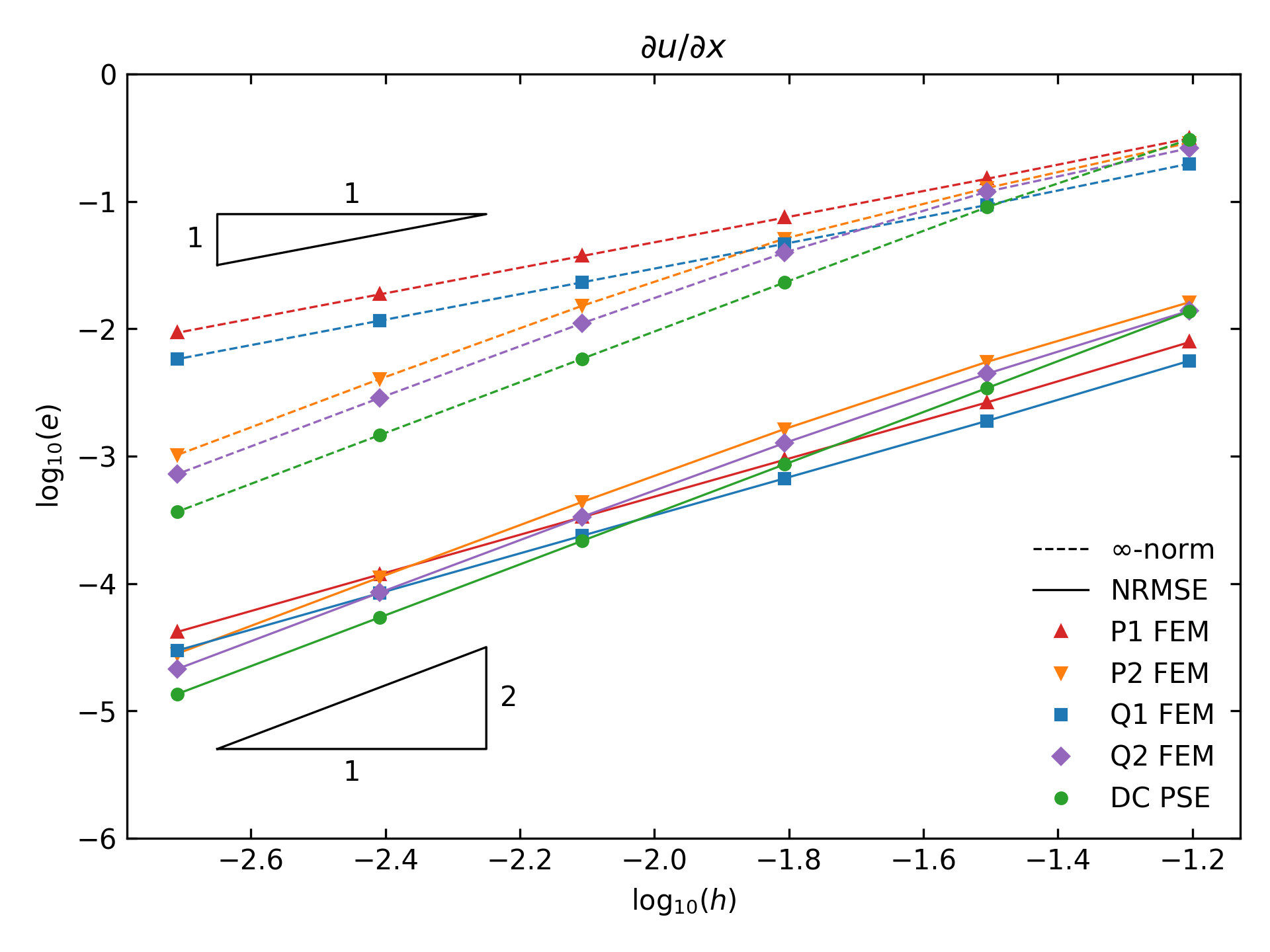
(a)

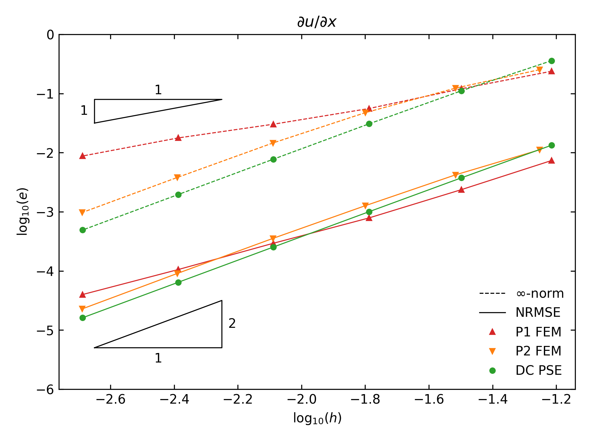
(b)

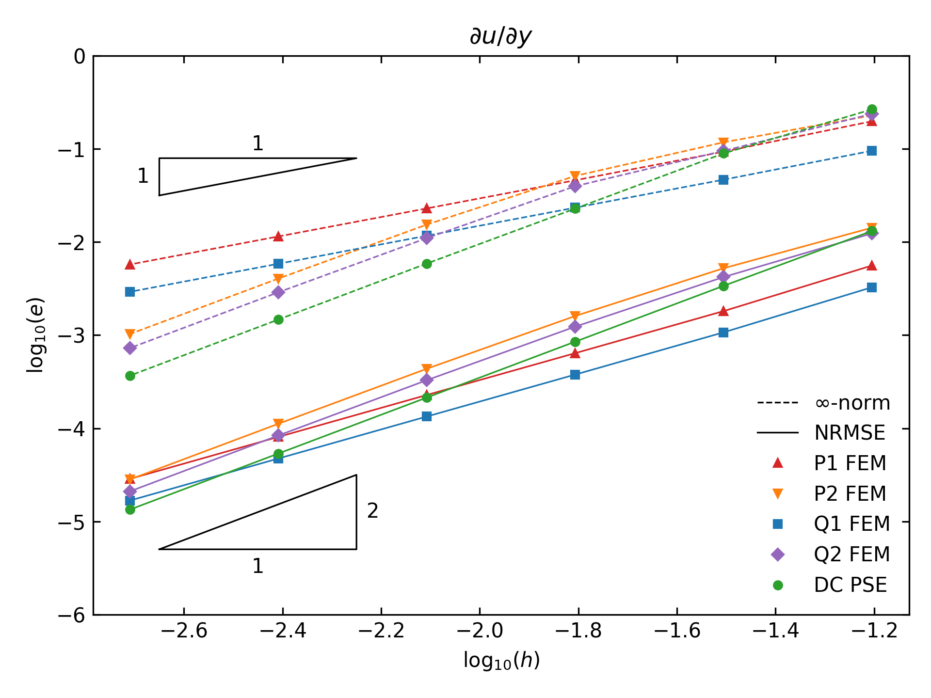
(c)

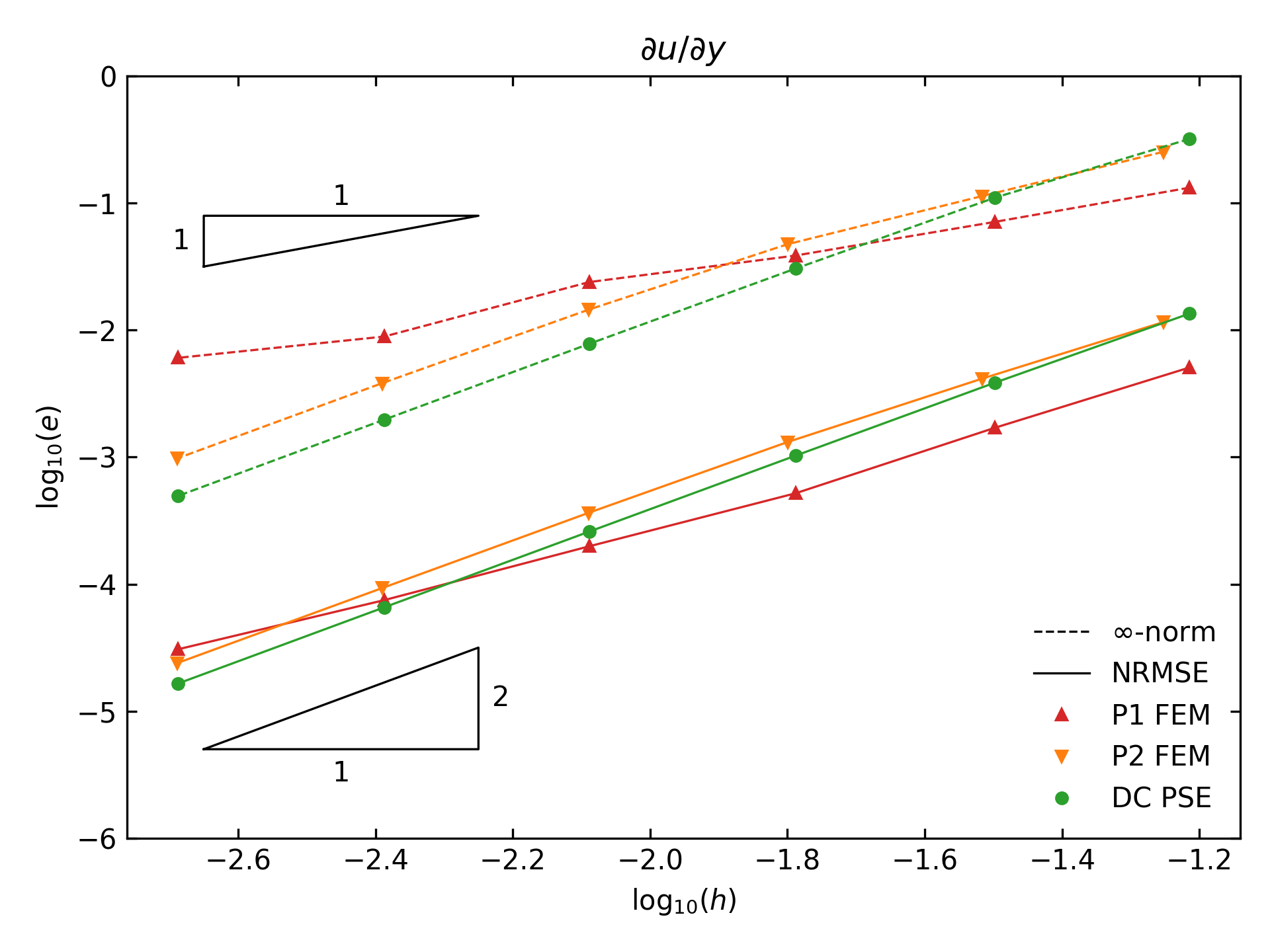
(d)

Figure 2: Convergence of numerical derivatives (a, b) $\mathrm{\partial}u/\mathrm{\partial}x$ and (c, d) $\mathrm{\partial}u/\mathrm{\partial}y$ of Franke’s function using (a, c) structured triangle and structured quadrilateral meshes and (b, d) unstructured triangle meshes. The derivatives were computed using linear (P1) and quadratic (P2) triangle finite elements, linear (Q1) and quadratic (Q2) quadrialteral finite elements, and the proposed meshfree DC PSE based method. The normalized node spacing $h$ for a 2D mesh with $n$ nodes is defined as $h=1/(n^{1/2}-1)$.

3.2 Infinite plate with a circular hole

The axially loaded infinite plate with a circular hole is a commonly used benchmark problem for stress analysis (Kelly et al., 1983; Zienkiewicz and Zhu, 1992; Boroomand and Zienkiewicz, 1997). The elastic stresses around the circumference of the hole are of primary interest and can be obtained analytically. The problem is applicable to infinitely thin structures such as a steel plate (plane stress) and infinitely thick structures such as a borehole (plane strain). The analytical solution for the planar stress is valid for both plane strain and plane stress. Here, we consider only plane strain loading conditions, where the displacement perpendicular to the plane of loading is assumed to be zero, because the stress recovery method requires the full displacement field for computing the strain and stress numerically.

The material is linear elastic with Young’s modulus $E=200$ GPa and Poisson’s ratio $\nu=0.3$. The analytical solution in polar coordinates $r,\theta$ for the displacement components—which applies only for plane strain—is given by (Timoshenko and Goodier, 1951)

$$u_{x}(r,\theta) =\frac{\sigma_{0}}{8\mu}\left(\frac{r}{a}(k+1)\mathrm{cos}\theta+\frac{2a}{r}((1+k)\mathrm{cos}\theta+\mathrm{cos}3\theta)-\frac{2a^{3}}{r^{3}}\mathrm{cos}3\theta\right),$$ (27)

$$u_{y}(r,\theta) =\frac{\sigma_{0}}{8\mu}\left(\frac{r}{a}(k-3)\mathrm{sin}\theta+\frac{2a}{r}((1-k)\mathrm{sin}\theta+\mathrm{sin}3\theta)-\frac{2a^{3}}{r^{3}}\mathrm{sin}3\theta\right),$$ (28)

where $\sigma_{0}$ is the far field traction and the Kolosov constant $k=3-4\nu$ for plane strain, with $\mu=E/(2(1+\nu))$ and $\nu$ being Lamé’s second parameter (shear modulus) and Poisson’s ratio, respectively. The analytical solution for the stress in the plane—valid for both plane strain and plane stress—is given by the Kirsch equations (Timoshenko and Goodier, 1951; Kirsch, 1898)

$$\sigma_{xx}(r,\theta) =\sigma_{0}\left[1-\frac{a^{2}}{r^{2}}\left(\frac{3}{2}\mathrm{cos}\,2\theta+\mathrm{cos}\,4\theta\right)+\frac{3a^{4}}{2r^{4}}\mathrm{cos}\,4\theta\right],$$ (29)

$$\sigma_{yy}(r,\theta) =\sigma_{0}\left[-\frac{a^{2}}{r^{2}}\left(\frac{1}{2}\mathrm{cos}\,2\theta-\mathrm{cos}\,4\theta\right)-\frac{3a^{4}}{2r^{4}}\mathrm{cos}\,4\theta\right],$$ (30)

$$\sigma_{xy}(r,\theta) =\sigma_{0}\left[-\frac{a^{2}}{r^{2}}\left(\frac{1}{2}\mathrm{sin}\,2\theta+\mathrm{sin}\,4\theta\right)+\frac{3a^{4}}{2r^{4}}\mathrm{sin}\,4\theta\right].$$ (31)

Fig. 3 shows some representative meshes used for this problem.

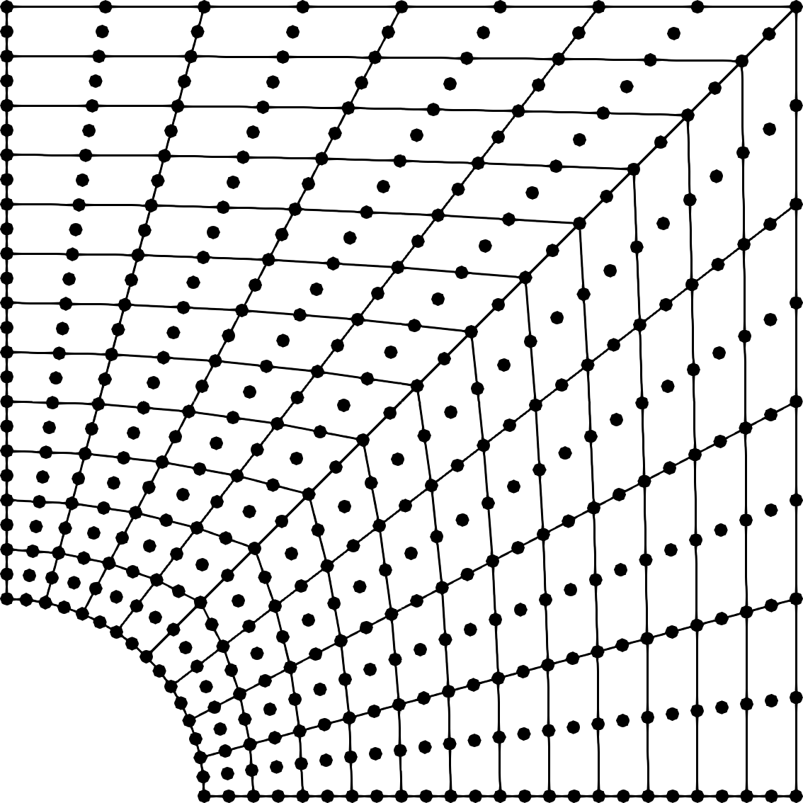
(a)

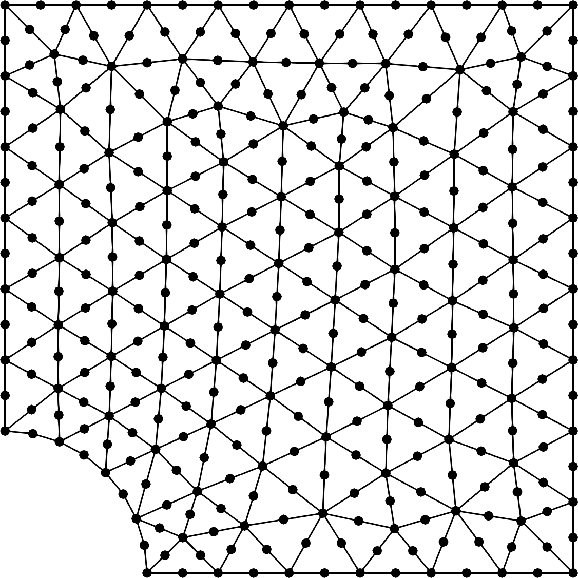
(b)

Figure 3: The (a) coarsest structured quadratic quadrilateral (Q2) mesh with 425 nodes ($h=0.051$) and 96 elements, and (b) coarsest unstructured quadratic triangle (P2) mesh with 357 nodes ($h=0.056$) and 162 elements used for the infinite plate with hole benchmark problem. The coarsest linear quadrilateral and triangle meshes have a similar number of nodes with more elements.

Using the analytical solution for the displacements at the nodal points, we computed the derivatives and derived quantities (strain and stress) numerically using the FE method with nodal averaging and the proposed DC PSE based meshfree recovery method to compare the accuracy of the stress components. Fig. 4 shows the convergence of each stress component computed at the nodal points. As expected, we observe first and second order convergence for the linear (P1 and Q1) and quadratic (P2 and Q2) finite elements, respectively. The stress computed using DC PSE converges at the same rate, and has similar accuracy, as the quadratic finite elements.

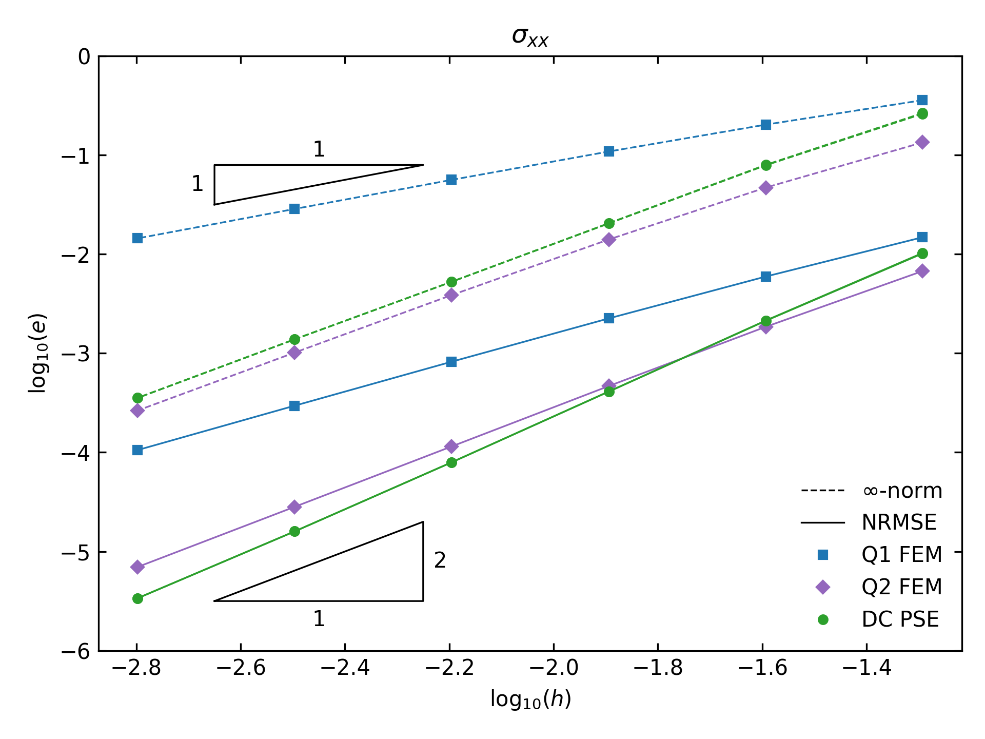
(a)

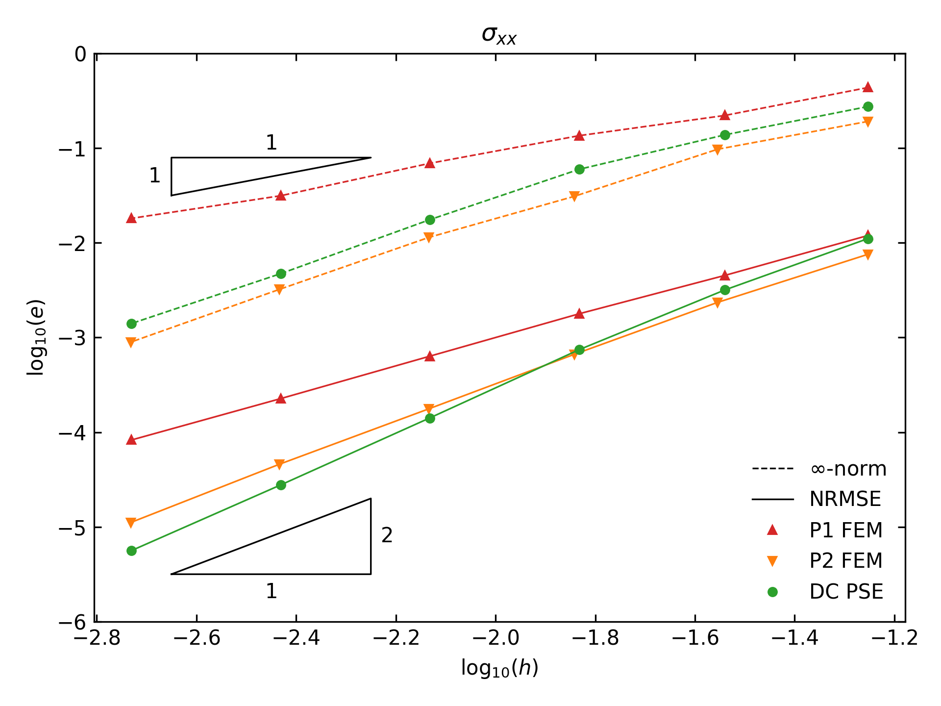
(b)

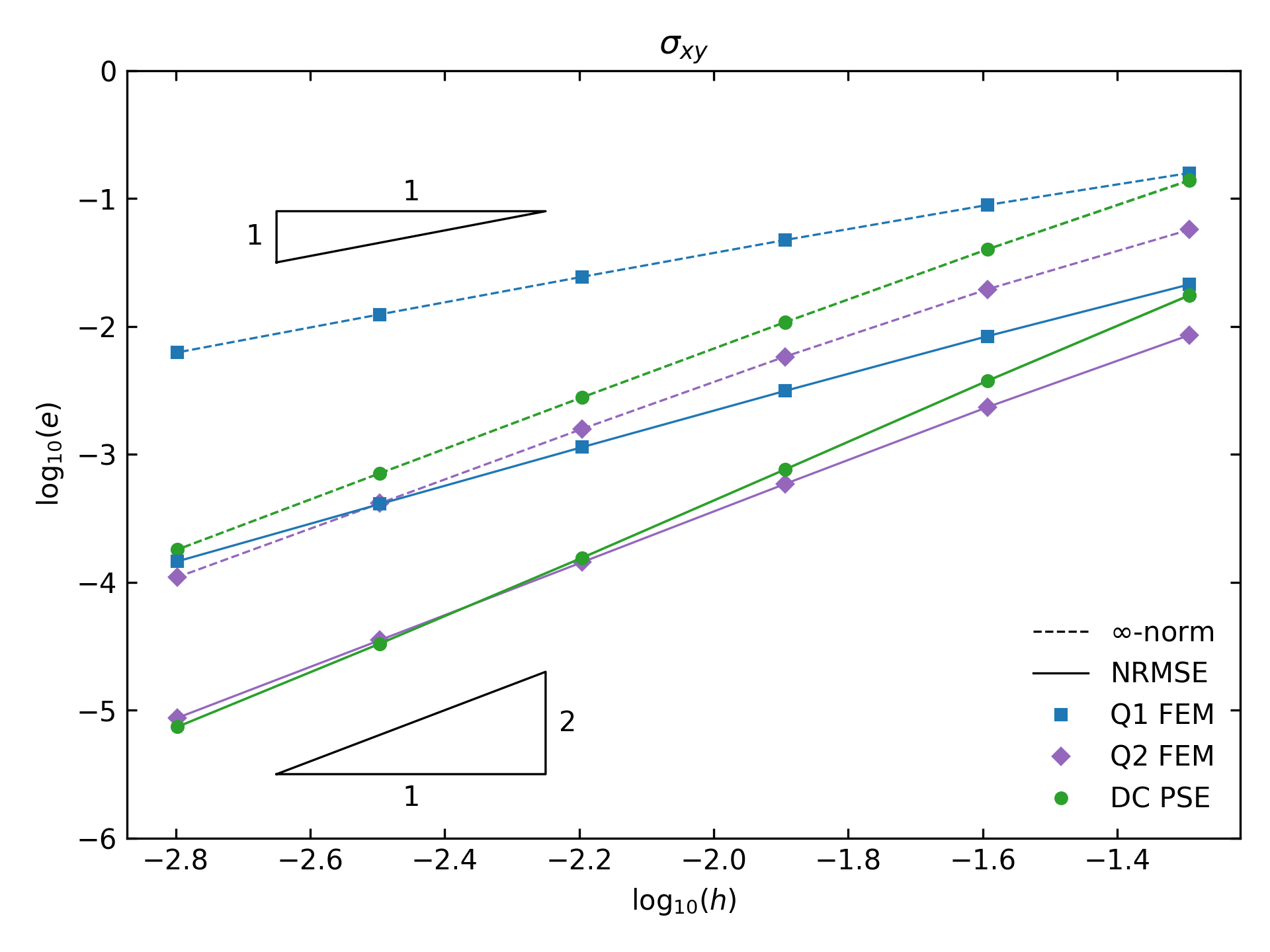
(c)

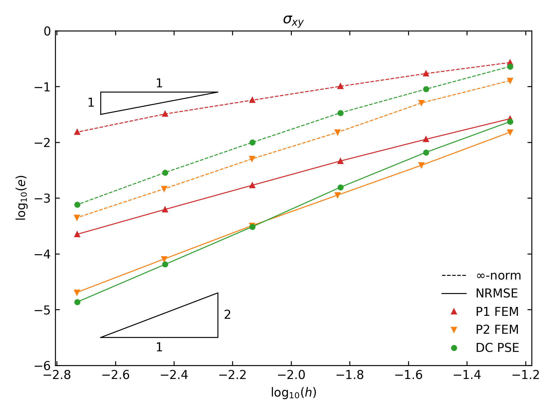
(d)

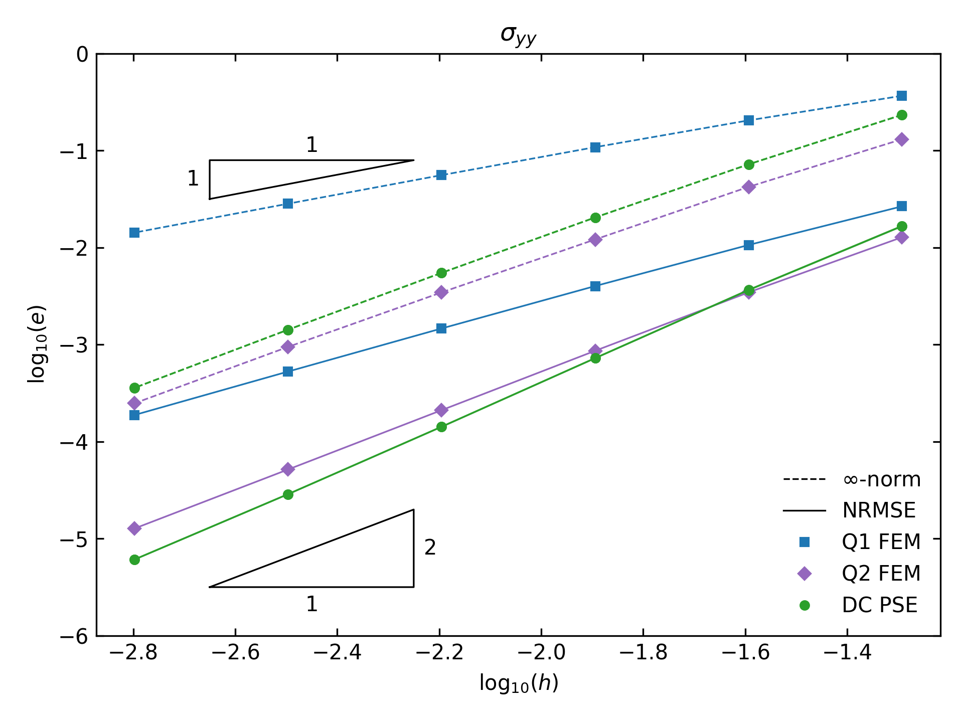
(e)

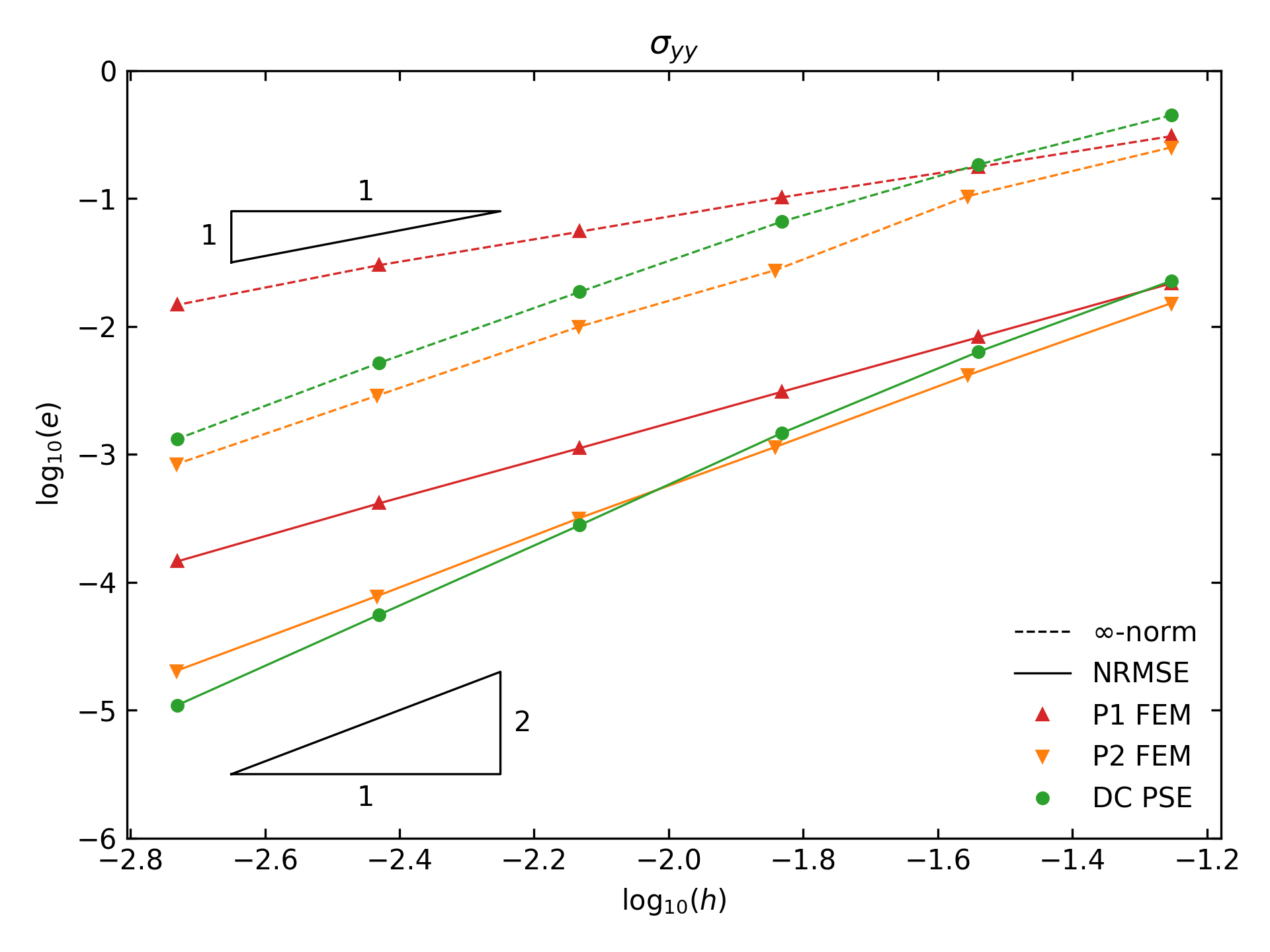
(f)

Figure 4: Convergence of stress components $\sigma_{xx}$, $\sigma_{xy}$ and $\sigma_{yy}$ for the infinite plate with hole benchmark problem using (a, c, e) structured quadrilateral and (b, d, f) unstructured triangle meshes. The normalized node spacing $h$ for a 2D mesh with $n$ nodes is defined as $h=1/(n^{1/2}-1)$.

3.3 3D cantilever beam

As a benchmark 3D example, we consider a rectangular beam with length $L=10$ cm, width $2a=2$ cm and height $2b=2$ cm. The beam is fixed (weakly) on the end $z=L$ and subjected to a transverse shear force $F=1$ N in the negative $y$-direction at the opposite end where $z=0$ (Bishop, 2014). The material is linear elastic with Young’s modulus $E=10^{7}$ N/cm² and Poisson’s ratio $\nu=0.3$. The analytical solution (Barber, 2010; Bishop, 2014) is given as follows for the displacement field:

$$u_{x}=-\frac{F\nu}{EI}xyz,$$ (32)

$$u_{y}=\frac{F}{EI}\left[\frac{\nu}{2}(x^{2}-y^{2})z-\frac{1}{6}z^{3}\right],$$ (33)

$$\begin{split}u_{z}=\frac{F}{EI}\left[\frac{1}{2}y(\nu x^{2}+z^{2})+\frac{1}{6}\nu y^{3}+(1+\nu)\left(b^{2}y-\frac{1}{3}y^{3}\right)-\frac{1}{3}a^{2}\nu y\right.\\ \left.-\frac{4a^{3}\nu}{\pi^{3}}\sum_{n=1}^{\infty}\frac{(-1)^{n}}{n^{3}}\mathrm{cos}(n\pi x/a)\frac{\mathrm{sinh}(n\pi y/a)}{\mathrm{cosh}(n\pi b/a)}\right],\end{split}$$ (34)

and for the stress field:

$$\sigma_{xx}=\sigma_{xy}=\sigma_{yy}=0,$$ (35)

$$\sigma_{zz}=\frac{F}{I}yz,$$ (36)

$$\sigma_{xz}=\frac{F}{I}\frac{2a^{2}}{\pi^{2}}\frac{\nu}{1+\nu}\sum_{n=1}^{\infty}\frac{(-1)^{n}}{n^{2}}\mathrm{sin}(n\pi x/a)\frac{\mathrm{sinh}(n\pi y/a)}{\mathrm{cosh}(n\pi b/a)},$$ (37)

$$\sigma_{yz}=\frac{F}{I}\frac{b^{2}-y^{2}}{2}+\frac{F}{I}\frac{\nu}{1+\nu}\left[\frac{3x^{2}-a^{2}}{6}-\frac{2a^{2}}{\pi^{2}}\sum_{n=1}^{\infty}\frac{(-1)^{n}}{n^{2}}\mathrm{cos}(n\pi x/a)\frac{\mathrm{cosh}(n\pi y/a)}{\mathrm{cosh}(n\pi b/a)}\right],$$ (38)

where $I=4ab^{3}/3$ is the second moment of area about the $x$-axis.

Fig. 5 shows some representative meshes used for this problem.

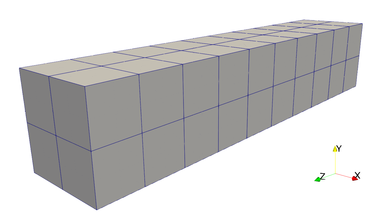
(a)

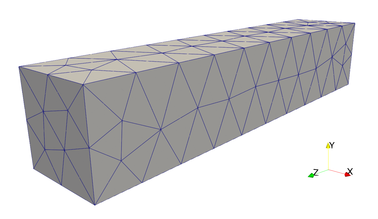
(b)

Figure 5: The (a) coarsest structured quadratic hexahedral (Q2) mesh with 525 nodes ($h=0.1415$) and 40 elements, and (b) coarsest unstructured quadratic tetrahedral (P2) mesh with 587 nodes ($h=0.1356$) and 260 elements used for the 3D cantilever benchmark problem. The coarsest linear hexahedral and tetrahedral meshes have a similar number of nodes with more elements.

Using the analytical solution for the displacements at the nodal points, we computed the derivatives and derived quantities (strain and stress) numerically using the FE method with nodal averaging and the proposed DC PSE based meshfree recovery method. Fig. 6 shows the errors in the nonzero stress components. The proposed DC PSE recovery method performs well compared to the FE method, with similar convergence rate and accuracy as quadratic finite elements. The $\sigma_{zz}$ stress component varies linearly with respect to $y$ and $z$, and is reproduced exactly by quadratic hexahedrons (the error is less than $10^{-6}$ for all $h$ tested) but not by linear finite elements or DC PSE. For unstructured tetrahedral meshes the DC PSE method appears to be slightly more accurate than the FE method with nodal averaging. This suggests that DC PSE may be useful in practical applications where complicated geometries cannot be meshed using a regular grid of hexahedral elements.

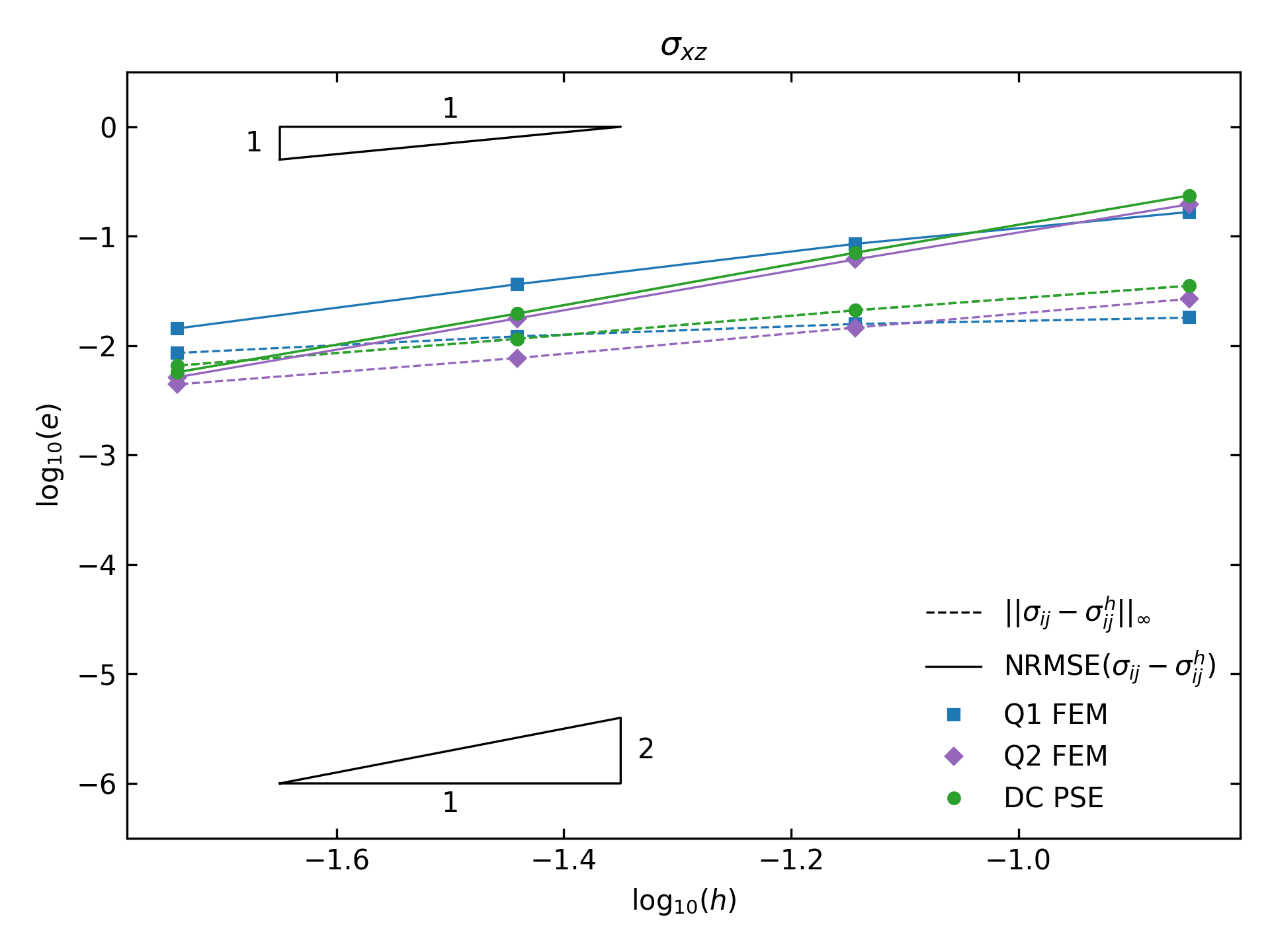
(a)

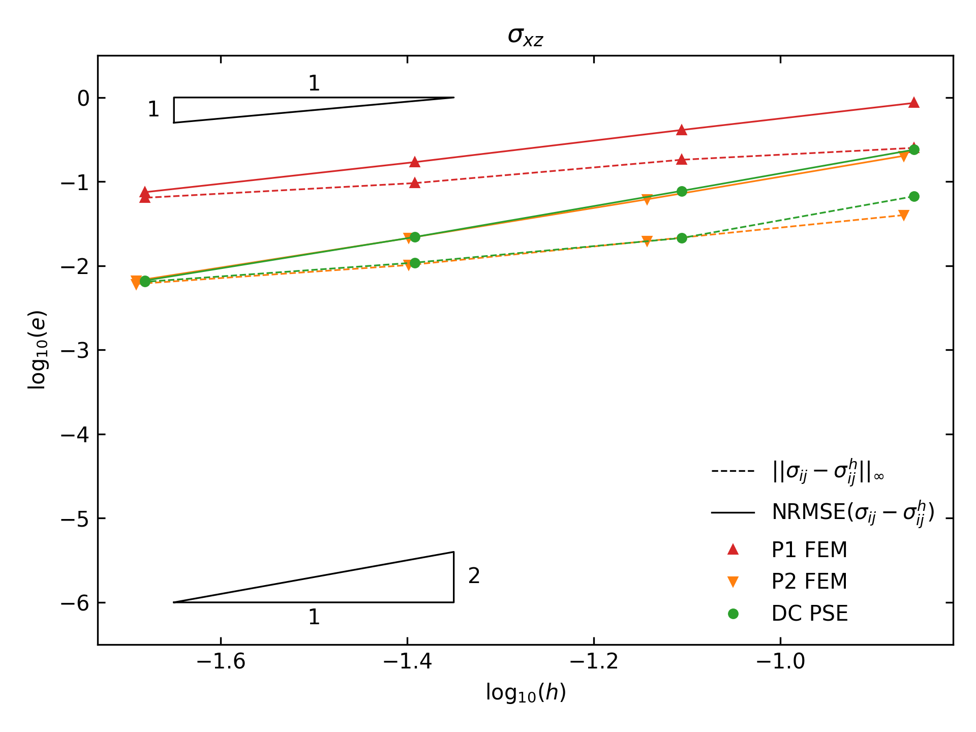
(b)

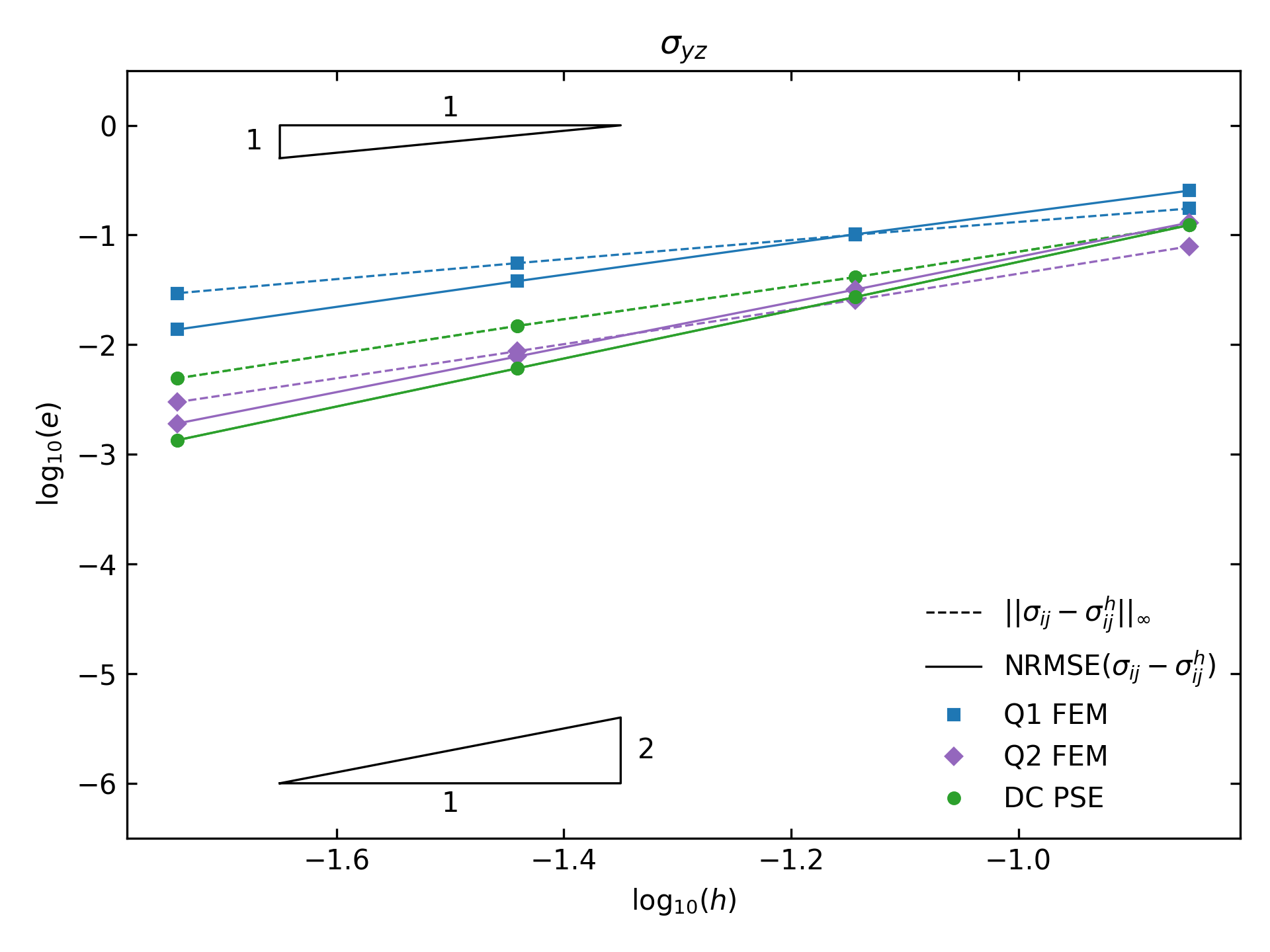
(c)

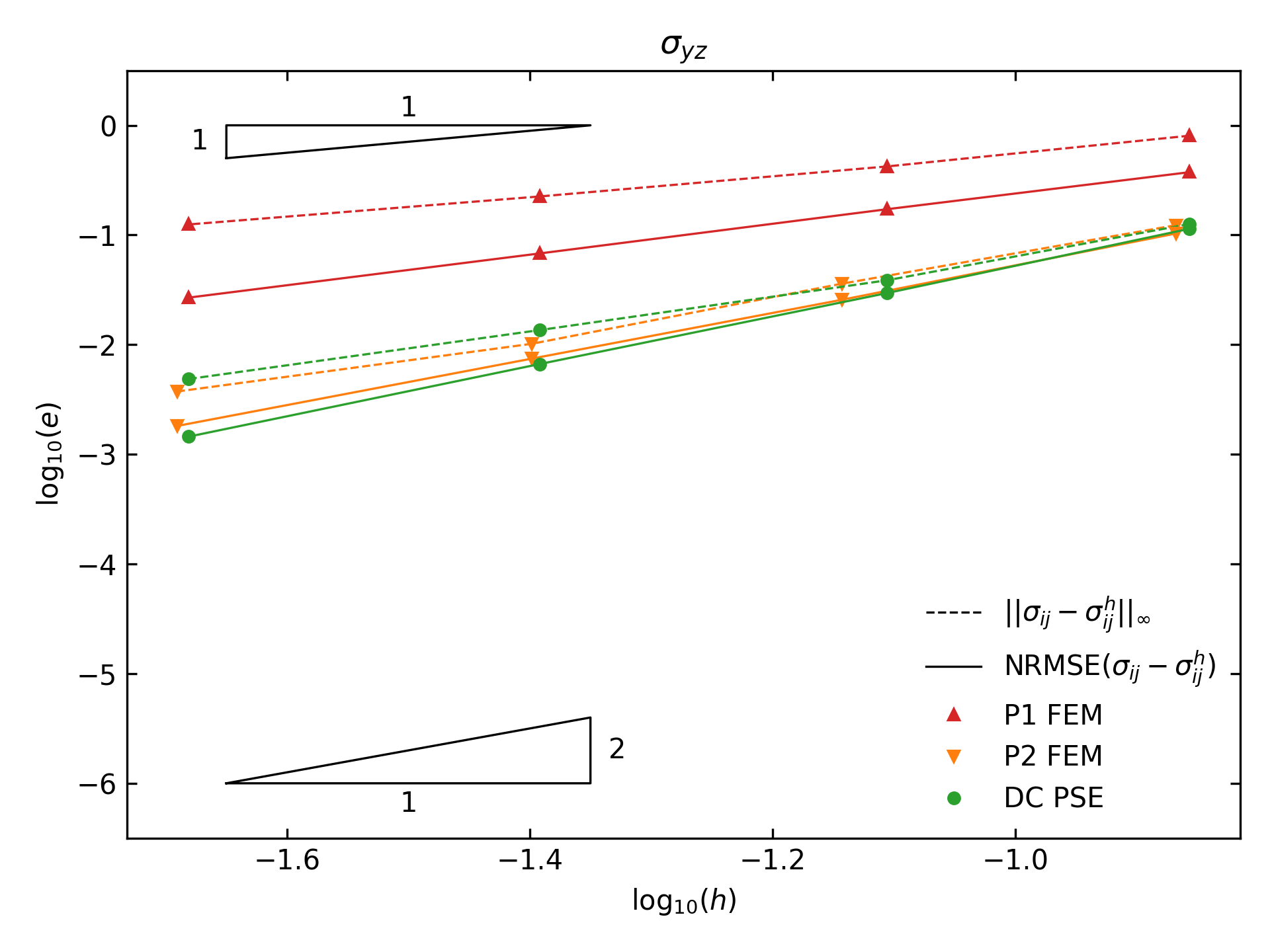
(d)

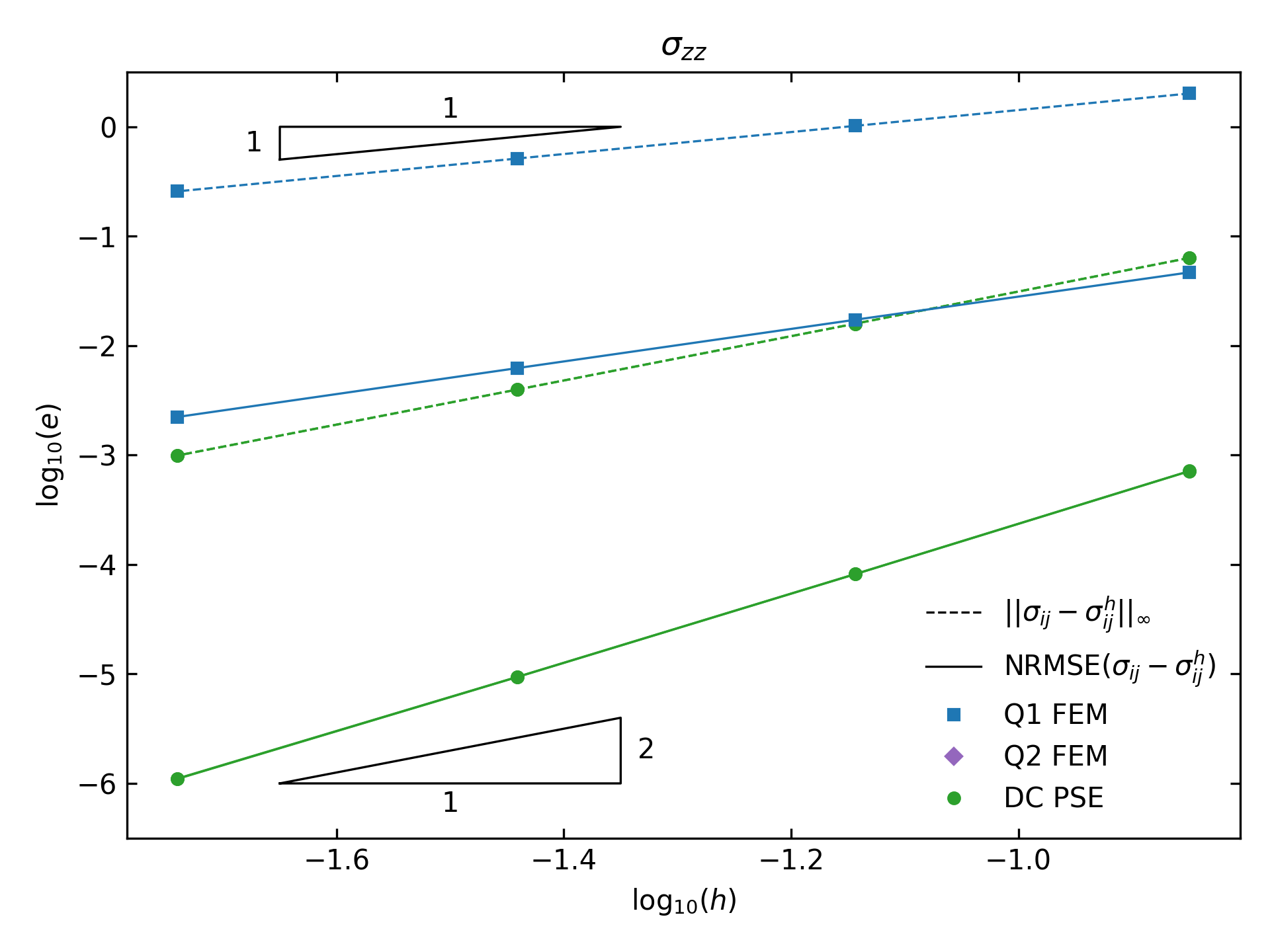
(e)

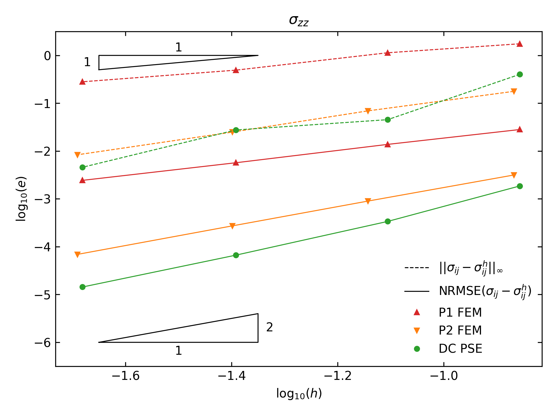
(f)

Figure 6: Convergence of stress components $\sigma_{xz}$, $\sigma_{yz}$ and $\sigma_{zz}$ for the 3D cantilever benchmark problem using (a, c, e) structured hexahedral and (b, d, f) unstructured tetrahedral meshes. The normalized node spacing $h$ for a 3D mesh with $n$ nodes is defined as $h=1/(n^{1/3}-1)$.

3.4 Stress in abdominal aortic aneurysm (AAA)

An abdominal aortic aneurysm (AAA) is an abnormal enlargement of the aorta, which is the main blood vessel that delivers blood to the body. Rupture of an AAA can have fatal consequences which means that patients must have periodic monitoring and, potentially, surgical intervention to repair the aneurysm. Stress analysis of aneurysms has been proposed as a risk assessment method for rupture (Joldes et al., 2017). The maximum stress often occurs on the inner or outer surface of the aneurysm wall. However, in the FE method, the stress is typically computed at the integration points which are located within the interior of the elements and, moreover, the normal component of stress across element boundaries is discontinuous. Stress recovery methods are required to obtain a smooth stress field and accurate stresses on the surface nodes of the aneurysm wall. In this example, we demonstrate the application of our proposed approach to the computation of stress in the arterial wall given a pre-computed displacement field. Here, we use the FEM to compute the displacement and compare the stress computed using FEM with that obtained using DC PSE.

The aneurysm geometry was extracted from a computed tomography (CT) scan using an image-based segmentation process. The open source mesh generator Gmsh (Geuzaine and Remacle, 2009) was used to create a mesh of the aneurysm wall with 521,441 quadratic tetrahedral elements and 928,682 nodes. We used Altair HyperMesh (https://www.altair.com/hypermesh) to check the element quality with the volumetric skew measure, which is a volume ratio between an ideal shaped equilateral tetrahedron and the tested actual tetrahedron. The volumetric skew measure ranges between 0 and 1, with 0 being an equilateral tetrahedron and 1 being a co-planar tetrahedron. For the AAA mesh considered in this example, all tetrahedra had volumetric skew less than 0.98. To model the material behavior of the aneurysm wall we used a linear elastic material with Young’s modulus $E=60$ MPa and Poisson’s ratio $\nu=0.45$ (Karimi et al., 2013). We used Abaqus/Standard to compute the displacements and stresses using the finite element method with quadratic tetrahedral displacement-based elements (C3D10 element type in Abaqus).

Fig. 7 shows the von Mises stress distribution computed using the FEM with nodal averaging compared to that computed using the proposed DC PSE meshfree approach. The stress distributions computed using the two methods are very similar but upon close inspection it is apparent that the DC PSE solution is smoother in some regions.

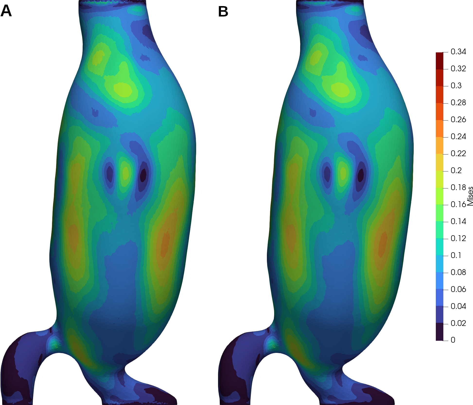
Figure 7: Distribution of von Mises stress on the outer wall of the abdominal aortic aneurysm (AAA). The displacement was computed using FEM with quadratic tetrahedral elements, and the stress was recovered using (a) FEM with nodal averaging and (b) meshfree DC PSE.

Table 1 shows the NRMSE between the stress components computed using FEM and those computed using the meshfree DC PSE based recovery method. The difference between the stress components computed using the FEM and DC PSE is less than $1\%$. Given that for the benchmark problems above the stress computed using quadratic tetrahedral elements with nodal averaging was slightly less accurate compared to DC PSE, we may believe that the results for the stress in the AAA computed using DC PSE should also be more accurate than those computed using FEM with nodal averaging.

Table 1: Normalized root mean square error (NRMSE) between the stress components computed using FEM and those computed using the DC PSE based recovery method for the abdominal aortic aneurysm (AAA) example problem.

Variable	NRMSE
$\sigma_{xx}$	9.51$\times 10^{-3}$
$\sigma_{xy}$	2.38$\times 10^{-3}$
$\sigma_{xz}$	4.11$\times 10^{-3}$
$\sigma_{yy}$	9.53$\times 10^{-3}$
$\sigma_{yz}$	3.52$\times 10^{-3}$
$\sigma_{zz}$	7.78$\times 10^{-3}$
$\sigma_{\mathrm{Mises}}$	5.80$\times 10^{-3}$

4 Discussion

We presented a novel recovery method based on DC PSE derivative operators. The DC PSE method is a truly meshfree method that does not require nodal connectivity defined by elements or the construction of element patches. The recovery procedure requires only the nodal points and nodal values of the primary variables to compute gradients and strains. When the constitutive material model and its parameters are known the stresses can also be computed. This allows the method to be easily incorporated into existing finite element software or used as a standalone post-processing tool.

To assess the accuracy of the proposed approach we compared its results with those obtained using the finite element method for a number of benchmark problems, before demonstrating the application of the method to a practical problem with complicated geometry by computing the stress within the wall of an aneurysm. In most cases, the meshless approach provides superior estimates of the gradient and other derived quantities compared to the FE method with nodal averaging. There are of course more sophisticated mesh-based methods that can be used to obtain more accurate gradients than nodal averaging, however, one of the salient advantages of the proposed method is that the gradient can be computed with accuracy similar to quadratic finite elements using a mesh of linear elements with a similar number of nodes. This is because the nodal connectivity is not required in our approach and the accuracy depends only on the density of the nodal distribution. Therefore, if the solution (displacement) can be computed with high accuracy using a dense mesh of linear elements, its gradient (and derived quantities of strain and stress) can be computed using the meshless DC PSE method with similar accuracy as if a coarser mesh of quadratic elements with a similar number of nodes was used to compute the solution and its gradient. This has significant practical importance in problems with complicated geometries that are reconstructed from image data with the boundaries triangulated using linear triangular elements. In these cases it is often difficult or impractical to generate a high quality mesh using higher order elements with curved edges that accurately capture the geometry of the boundary.

The new recovery method based on the DC PSE formulation is general and can be used for both linear and nonlinear problems. Higher order derivatives than those used in the current study can also be easily computed using the DC PSE method. Although in this study we considered only the equations of linear elasticity, the recovery method can be easily applied to other boundary value problems such as nonlinear solid mechanics and the Navier–Stokes equations by simply modifying the equations used to compute the derived quantities given the gradient obtained using DC PSE. An important quantity of interest in fluid flow simulations is the wall shear stress (Gijsen et al., 2019). In many practical applications the velocity field is obtained using piecewise linear (P1) elements which makes accurate recovery of the gradient a difficult task (Valen-Sendstad and Steinman, 2014). This task may be simplified by the adoption of the recovery procedure presented and we intend to investigate the accuracy of this approach in our future studies.

The proposed recovery procedure may be applied as a recovery-based error estimator (Ainsworth and Oden, 2000) whereby the discontinuous finite element solution at the element nodes is compared to the continuous solution obtained using the DC PSE operators. This error estimator could be used in adaptive mesh refinement algorithms in both finite element and meshless methods. The advantage of this approach over existing element-based methods is that patches do not need to be created thereby simplifying the implementation, especially when using complex meshes consisting of various element shapes.

The meshfree gradient recovery approach that we have described in this paper has many practical applications. Its simplicity, and the fact that it does not rely on predefined connectivity between neighboring nodes, makes it an ideal post-processing tool to be used as an “add-on” to existing simulation packages for improving the accuracy of stress and strain computations. We are now working on extending the approach described in this paper to other equations with practical significance with the aim of improving the estimation of derived quantities from accurate solutions of the primary solution variable(s) obtained using low order (typically linear) approximations that are often employed in practice.

References

- Ahmed (2020) Ahmed, M., 2020. A Comparative Study of Mesh-Free Radial Point Interpolation Method and Moving Least Squares Method-Based Error Estimation in Elastic Finite Element Analysis. Arabian Journal for Science and Engineering 45, 3541–3557. doi:10.1007/s13369-019-04154-5.
- Ahmed et al. (2018) Ahmed, M., Singh, D., Desmukh, M.N., 2018. Interpolation Type Stress Recovery Technique Based Error Estimator for Elasticity Problems. Mechanics 24, 672–679. doi:10.5755/j01.mech.24.5.19937.
- Ainsworth and Oden (2000) Ainsworth, M., Oden, J.T., 2000. A Posteriori Error Estimation in Finite Element Analysis. Pure and Applied Mathematics., Wiley, New York.
- Barber (2010) Barber, J.R., 2010. Elasticity. volume 172 of Solid Mechanics and Its Applications. Springer Netherlands, Dordrecht. doi:10.1007/978-90-481-3809-8.
- Bishop (2014) Bishop, J.E., 2014. A displacement-based finite element formulation for general polyhedra using harmonic shape functions. International Journal for Numerical Methods in Engineering 97, 1–31. doi:10.1002/nme.4562.
- Boroomand and Zienkiewicz (1997) Boroomand, B., Zienkiewicz, O.C., 1997. Recovery by Equilibrium in Patches (REP). International Journal for Numerical Methods in Engineering 40, 137–164. doi:10.1002/(SICI)1097-0207(19970115)40:1<137::AID-NME57>3.0.CO;2-5.
- Chen and Belytschko (2015) Chen, J.S., Belytschko, T., 2015. Meshless and Meshfree Methods, in: Engquist, B. (Ed.), Encyclopedia of Applied and Computational Mathematics. Springer Berlin Heidelberg, Berlin, Heidelberg, pp. 886–894. doi:10.1007/978-3-540-70529-1_531.
- Choi et al. (1991) Choi, D., Thorpe, J.L., Hanna, R.B., 1991. Image analysis to measure strain in wood and paper. Wood Science and Technology 25, 251–262. doi:10.1007/BF00225465.
- Fasshauer (2007) Fasshauer, G.E., 2007. Meshfree Approximation Methods with MATLAB. World Scientific, Singapore.
- Franke (1979) Franke, R., 1979. A Critical Comparison of Some Methods for Interpolation of Scattered Data. Technical Report. Monterey, California: Naval Postgraduate School. URL: https://calhoun.nps.edu/handle/10945/35052.
- Geuzaine and Remacle (2009) Geuzaine, C., Remacle, J.F., 2009. Gmsh: A 3-D finite element mesh generator with built-in pre- and post-processing facilities. International Journal for Numerical Methods in Engineering 79, 1309–1331. doi:10.1002/nme.2579.
- Gijsen et al. (2019) Gijsen, F., Katagiri, Y., Barlis, P., Bourantas, C., Collet, C., Coskun, U., Daemen, J., Dijkstra, J., Edelman, E., Evans, P., van der Heiden, K., Hose, R., Koo, B.K., Krams, R., Marsden, A., Migliavacca, F., Onuma, Y., Ooi, A., Poon, E., Samady, H., Stone, P., Takahashi, K., Tang, D., Thondapu, V., Tenekecioglu, E., Timmins, L., Torii, R., Wentzel, J., Serruys, P., 2019. Expert recommendations on the assessment of wall shear stress in human coronary arteries: Existing methodologies, technical considerations, and clinical applications. European Heart Journal 40, 3421–3433. doi:10.1093/eurheartj/ehz551.
- Joldes et al. (2017) Joldes, G.R., Miller, K., Wittek, A., Forsythe, R.O., Newby, D.E., Doyle, B.J., 2017. BioPARR: A software system for estimating the rupture potential index for abdominal aortic aneurysms. Scientific Reports 7, 4641. doi:10.1038/s41598-017-04699-1.
- Karimi et al. (2013) Karimi, A., Navidbakhsh, M., Faghihi, S., Shojaei, A., Hassani, K., 2013. A finite element investigation on plaque vulnerability in realistic healthy and atherosclerotic human coronary arteries. Proceedings of the Institution of Mechanical Engineers, Part H: Journal of Engineering in Medicine 227, 148–161. doi:10.1177/0954411912461239.
- Kelly et al. (1983) Kelly, D.W., Gago, J.P.D.S.R., Zienkiewicz, O.C., Babuska, I., 1983. A posteriori error analysis and adaptive processes in the finite element method: Part I—error analysis. International Journal for Numerical Methods in Engineering 19, 1593–1619. doi:10.1002/nme.1620191103.
- Kirsch (1898) Kirsch, G., 1898. Die Theorie der Elastizität und die Bedürfnisse der Festigkeitslehre. Zeitschrift des Vereines Deutscher Ingenieure 42, 797–807.
- Lee and Zhou (2004) Lee, C.K., Zhou, C.E., 2004. On error estimation and adaptive refinement for element free Galerkin method: Part I: Stress recovery and a posteriori error estimation. Computers & Structures 82, 413–428. doi:10.1016/j.compstruc.2003.10.018.
- López-Linares et al. (2019) López-Linares, K., García, I., García, A., Cortes, C., Piella, G., Macía, I., Noailly, J., González Ballester, M.A., 2019. Image-Based 3D Characterization of Abdominal Aortic Aneurysm Deformation After Endovascular Aneurysm Repair. Frontiers in Bioengineering and Biotechnology 7. doi:10.3389/fbioe.2019.00267.
- Oden and Brauchli (1971) Oden, J.T., Brauchli, H.J., 1971. On the calculation of consistent stress distributions in finite element approximations. International Journal for Numerical Methods in Engineering 3, 317–325. doi:10.1002/nme.1620030303.
- Reboux et al. (2012) Reboux, S., Schrader, B., Sbalzarini, I.F., 2012. A self-organizing Lagrangian particle method for adaptive-resolution advection–diffusion simulations. Journal of Computational Physics 231, 3623–3646. doi:10.1016/j.jcp.2012.01.026.
- Schrader (2011) Schrader, B., 2011. Discretization-Corrected PSE Operators for Adaptive Multiresolution Particle Methods. Doctoral Thesis. ETH Zurich. doi:10.3929/ethz-a-006425176.
- Schrader et al. (2010) Schrader, B., Reboux, S., Sbalzarini, I.F., 2010. Discretization correction of general integral PSE Operators for particle methods. Journal of Computational Physics 229, 4159–4182. doi:10.1016/j.jcp.2010.02.004.
- Schrader et al. (2012) Schrader, B., Reboux, S., Sbalzarini, I.F., 2012. Choosing the Best Kernel: Performance Models for Diffusion Operators in Particle Methods. SIAM Journal on Scientific Computing 34, A1607–A1634. doi:10.1137/110835815.
- Timoshenko and Goodier (1951) Timoshenko, S., Goodier, J.N., 1951. Theory of Elasticity. Second ed., McGraw-Hill, New York.
- Valen-Sendstad and Steinman (2014) Valen-Sendstad, K., Steinman, D.A., 2014. Mind the Gap: Impact of Computational Fluid Dynamics Solution Strategy on Prediction of Intracranial Aneurysm Hemodynamics and Rupture Status Indicators. American Journal of Neuroradiology 35, 536–543. doi:10.3174/ajnr.A3793.
- Zhang and Naga (2005) Zhang, Z., Naga, A., 2005. A New Finite Element Gradient Recovery Method: Superconvergence Property. SIAM Journal on Scientific Computing 26, 1192–1213. doi:10.1137/S1064827503402837.
- Zienkiewicz et al. (2013) Zienkiewicz, O.C., Taylor, R.L., Fox, D.D., 2013. The Finite Element Method for Solid and Structural Mechanics. Seventh ed., Butterworth-Heinemann.
- Zienkiewicz and Zhu (1987) Zienkiewicz, O.C., Zhu, J.Z., 1987. A simple error estimator and adaptive procedure for practical engineerng analysis. International Journal for Numerical Methods in Engineering 24, 337–357. doi:10.1002/nme.1620240206.
- Zienkiewicz and Zhu (1992) Zienkiewicz, O.C., Zhu, J.Z., 1992. The superconvergent patch recovery and a posteriori error estimates. Part 1: The recovery technique. International Journal for Numerical Methods in Engineering 33, 1331–1364. doi:10.1002/nme.1620330702.
- Zienkiewicz and Zhu (1995) Zienkiewicz, O.C., Zhu, J.Z., 1995. Superconvergence and the superconvergent patch recovery. Finite Elements in Analysis and Design 19, 11–23. doi:10.1016/0168-874X(94)00054-J.