Rydberg Atomic Antenna in Strongly Driven Multi-Electron Atoms

Abstract

We study the role of intermediate excitations of Rydberg states as an example of Kuchiev’s “atomic antenna” in above-threshold ionization of xenon, in particular their effect on the coherence between the spin–orbit-split states of the ion. We focus on the case of a laser frequency close to resonant with the spin–orbit splitting, where a symmetry (parity) argument would preclude any coherence being directly generated by strong-field ionization. Using ab initio simulations of coupled multielectron spin–orbit dynamics in strong laser fields, we show how field-driven rescattering of the trapped Rydberg electrons introduces efficient coupling between the spin–orbit-split channels, leading to substantial coherences, exceeding $10\text{\,}\mathrm{\char 37\relax}$ for some photon energies.

I Introduction

Spin–orbit effects are usually neglected in the interaction with strong infrared (IR) fields. Few exceptions include the development of consistent treatment within the $R$-matrix method [1], recent experiments [2, 3] on imaging the spin–orbit breathing of a hole created by strong-field ionization, and the generation of spin-polarized photoelectrons [4] following the proposal of [5, 6]. In all these cases [2, 3, 4, 5, 6], the dipole approximation holds, ensuring that no transitions between the spin–orbit-split states were induced by the incident IR field.

In this article we show that, even in the dipole approximation, strong IR fields trigger transitions between the spin–orbit-split states of the ion via a mechanism resembling the “atomic antenna” of Kuchiev [7]. In our case, an active electron driven by strong IR field is trapped into a long-lived Rydberg orbit. Oscillating in the IR field, it transfers the energy to the core via non-dipole electron–electron interaction. This atomic antenna breaks the dynamic symmetry with respect to the polarization of the linearly polarized driving laser field [8]. It thereby induces coherence between the spin–orbit-split states of the ion, reduces the entanglement between the ion and the photoelectron, and manifests itself in the photoelectron spectra.

This article is arranged as follows: in section II, we introduce the degree of coherence between ionic states, and discuss why parity-conservation arguments require the coherence to vanish, when the photon energy matches the spin–orbit splitting; in section III, we present the main computational results that contradict these expectations, as well as our explanation. Finally, section IV concludes the article.

II Theory

We consider a xenon atom, initially in the ground state, interacting with an IR pulse with carrier photon energy $\hbar\omega$ close to the spin–orbit splitting of the cation, $\Delta E_{\textrm{s--o}}\approx$1.3\text{\,}\mathrm{eV}$$, $\eta\overset{\textrm{\tiny def}}{=}\hbar\omega/\Delta E_{\textrm{s--o}}\sim 1$ (atomic units $\hbar=e=a_{0}=m_{\mathrm{e}}=1$ are used in the following). Our calculations include all relevant electronic excitations (i.e. single excitations/ionizations from $\mathrm{5s}_{1/2}$, $\mathrm{5p}_{1/2}$, or $\mathrm{5p}_{3/2}$ are allowed), and account for spin–orbit coupling effects. We solve the time-dependent Schrödinger equation in the dipole approximation and the length gauge, for a configuration-interaction singles Ansatz that allows single excitation/ionization from a Hartree–Fock (HF) reference [9, 10, 11, 12, 13, 14, *Carlstroem2022tdcisII]. The spin–orbit interaction is treated using an energy-consistent relativistic effective-core potential [16] (see [17] for an alternative option, based on the four-component Dirac equation). Ion-resolved above-threshold ionization (ATI) photoelectron spectra are computed [14, *Carlstroem2022tdcisII] using the tSURFF [18, 19, 20, 21, 22] and iSURFV [23] techniques. From these spectra, we compute the reduced density matrix $\{\rho_{IJ}\}$, obtained by tracing over the photoelectron degrees of freedom. We then form the normalized degree of coherence:

$$\tilde{\rho}_{IJ}\overset{\textrm{\tiny def}}{=}\frac{\rho_{IJ}}{\sqrt{\rho_{II}\rho_{JJ}}},$$ (1)

where $\rho_{IJ}$ is the coherence between $I$ and $J$, and $\rho_{II}$ and $\rho_{JJ}$ are the populations in the ion states $I$ and $J$, respectively. Further details are given in Appendix A.

Let us first consider coherence between the spin–orbit-split states of the ion generated by ionization [3, 6, 24, 25, 26, 27]. The final state of the system “ion+photoelectron” is

$$\ket{\Psi} =\ket*{I}\!\!\ket*{\chi_{I}}+\ket*{J}\!\!\ket*{\chi_{J}}$$ (2)

$$=(\ket*{I}+\ket*{J}w)\ket*{\chi_{I}}+\ket*{J}(\ket*{\chi_{J}}-w\ket*{\chi_{I}}),$$

where we choose $w\overset{\textrm{\tiny def}}{=}\innerproduct*{\chi_{I}}{\chi_{J}}$ as a measure of the factorizability of the wavefunction, and antisymmetrization with respect to the coordinates of the photoelectron is implied. Coherent spin–orbit dynamics in the ion requires non-zero overlap between the continuum electron wavepackets correlated to the ionic states $\ket*{I}$ and $\ket*{J}$, respectively: $w\neq 0$. Perfect overlap $\left|w\right|=1$ corresponds to $100\text{\,}\mathrm{\char 37\relax}$ degree of coherence, since (2) factorizes into

$$\ket{\Psi}=(\ket*{I}+\mathrm{e}^{\mathrm{i}\phi}\ket*{J})\ket*{\chi},$$

for some phase $\phi$. Perfect electron–ion entanglement corresponds to $w=0$.

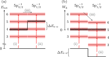
Figure 1: Sketch of the energy diagram for ATI from xenon for $\eta\overset{\textrm{\tiny def}}{=}\hbar\omega/\Delta E_{\textrm{s--o}}=0.9$; the numbers indicate the amount of photons necessary to reach a certain final energy. The three most important pathways are: (i) direct ionization into the ${\mathrm{5p}}^{-1}_{3/2}$ channel including elastic rescattering, (ii) direct ionization/elastic rescattering in the ${\mathrm{5p}}^{-1}_{1/2}$ channel, and (iii) indirect contributions due to inelastic rescattering from ${\mathrm{5p}}^{-1}_{3/2}$ to ${\mathrm{5p}}^{-1}_{1/2}$ (this dominates over rescattering in the other direction). (a) Total energy (photoelectron + ion), relative to the field-free neutral atom. In this picture, the energy conservation in inelastic scattering is easily seen. (b) Energies of the photoelectrons in each channel. Non-zero photoelectron overlap is necessary for a coherence between the ion cores to exist. For $\eta\sim 1$, photoelectrons of similar kinetic energies are due to absorption of a different number of photons.

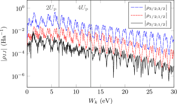
Figure 2: Calculated ATI spectrum of xenon using $4.4\text{\times}{10}^{13}\text{\,}\mathrm{W}\text{\,}{\mathrm{cm}}^{-2}$ with $\eta\approx 0.96$ and a pulse duration of $30\text{\,}\mathrm{fs}$. The dashed blue line is the photoelectron spectrum $\rho_{3/2;3/2}$ correlated with the ${\mathrm{5p}}^{-1}_{3/2}$ ionization channel; the dot-dashed red line the corresponding spectrum $\rho_{1/2;1/2}$ for the ${\mathrm{5p}}^{-1}_{1/2}$ channel; and the black solid line is the energy-resolved coherence $\rho_{3/2;1/2}$ between the two channels. Above approximately $4U_{\mathrm{p}}$, the spectrum in ${\mathrm{5p}}^{-1}_{1/2}$ and the coherence exhibit structures which are very similar to the spectrum in ${\mathrm{5p}}^{-1}_{3/2}$; we infer that the ${\mathrm{5p}}^{-1}_{1/2}$ channel is populated almost exclusively through rescattering in this energy region [see (iii) in Figure 1].

By a symmetry argument, zero coherence and perfect entanglement are expected for $\eta=1$: non-zero coherence and hence $w\neq 0$ requires that the two photoelectron wavepackets overlap in energy. After absorption of $q$ photons of energy $\omega$, the photoelectron energy is

$$W_{k}=q\omega-I_{\mathrm{p},{I}}-U_{\mathrm{p}}-\frac{\delta\alpha_{I}}{4}F^{2}=q\omega-I_{\mathrm{p},{I}}-U_{\mathrm{p}}(1+\omega^{2}\delta\alpha_{I}),$$ (3)

where $\omega$ is the driving laser frequency, $I_{\mathrm{p},{I}}$ is the ionization potential in ionization channel $I$, $U_{\mathrm{p}}=F^{2}/4\omega^{2}$ the ponderomotive potential of the electric field with peak amplitude $F$, and $\delta\alpha_{I}$ the difference between the polarizabilities of the ground state of the neutral and the state of the ion. For $\eta\sim 1$, the photoelectron peaks correlated to the ${\mathrm{5p}}^{-1}_{3/2}$ and ${\mathrm{5p}}^{-1}_{1/2}$ ion cores coincide in energy when one extra photon is absorbed in the ${\mathrm{5p}}^{-1}_{1/2}$ channel (see Figure 1). Thus, the photoelectron associated with ${\mathrm{5p}}^{-1}_{3/2}$ would have opposite parity compared to ${\mathrm{5p}}^{-1}_{1/2}$, while the ${\mathrm{5p}}^{-1}_{3/2}$ and ${\mathrm{5p}}^{-1}_{1/2}$ ion cores have the same parity. The overall parity would thus be opposite between the channels, implying $w=0$ by symmetry, precluding any coherence. If very short, broadband pulses are used, a non-zero coherence can nonetheless result, due to the energetic overlap of two successive ATI peaks belonging to the two thresholds. This is the mechanism behind the coherence observed by Goulielmakis et al. [3], who use pulses of $3.8\text{\,}\mathrm{fs}$ duration. This coherence diminishes when longer pulses are used, and is expected to disappear entirely for the much longer pulses ($\geq$15\text{\,}\mathrm{fs}$$) used in the present work.

III Results

We begin by considering ionization by a $30\text{\,}\mathrm{fs}$ pulse, tuned just below the spin–orbit splitting ($\eta=0.96$). As can be seen from the simulation results in Figure 2, there is non-zero coherence between ${\mathrm{5p}}^{-1}_{3/2}$ and ${\mathrm{5p}}^{-1}_{1/2}$, where the ATI peaks in the respective channels overlap energetically.

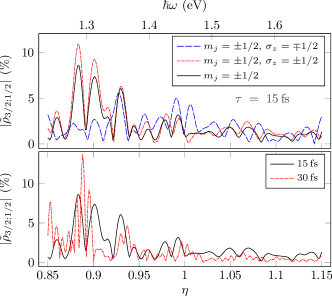
Figure 3: Ionic coherence in xenon. Upper panel: the degree of coherence [Eq. (1)] between the ionization channels ${\mathrm{5p}}^{-1}_{3/2}$ and ${\mathrm{5p}}^{-1}_{1/2}$ as a function of the ratio $\eta$ between the photon energy and the spin–orbit splitting, resolved on the $m_{j}$ quantum number of the ion and the spin $\sigma_{z}$ of the photoelectron. Due to the cylindrical symmetry of the ionization process, there is a mirror symmetry in the combinations of $m_{j}$ and $\sigma_{z}$. Additionally tracing out $\sigma_{z}$ leads to the final degrees of coherence for $m_{j}=\pm 1/2$, which coincide. Lower panel: the degree of coherence for two different pulse durations; solid black line: $\tau=$15\text{\,}\mathrm{fs}$$, dot-dashed red line: $\tau=$30\text{\,}\mathrm{fs}$$.

Figure 3 shows the calculated degree of coherence (1) between the ${\mathrm{5p}}^{-1}_{3/2}$ and ${\mathrm{5p}}^{-1}_{1/2}$ ion cores, as a function of $\eta$. Contrary to the symmetry-based expectation, we see substantial coherence, even exceeding $10\text{\,}\mathrm{\char 37\relax}$ for some $\eta$. We trace its origin to frustrated tunnelling [28, 29, 30] — trapping of the electron into Rydberg states after optical tunnelling from the ground state. Once the neutral atom is “parked” in the intermediate, excited state for an extended amount of time, there is an opportunity to undergo multiple successive (Stokes–)Raman transitions that each increase the system energy by a small amount, while conserving the parity. After multiple such Raman transitions have occured, the energy may increase enough to bridge the energy gap to the next ATI order. Upon subsequent ionization and rescattering into the other ion channel, the overlap of photoelectrons of the same parity and energy explains the observed coherence.

In the frequency domain, frustrated tunnelling followed by ionization corresponds to the so-called Freeman resonances [31] imprinted on top of the photoelectron peaks. The apparent “parity violation” is a manifestation of the dynamic symmetry being broken due to the simultaneous presence of the Freeman resonances, and the spin–orbit interaction. The Freeman resonances introduce memory in the time evolution, breaking time-reversal symmetry, or equivalently, spatial inversion symmetry between the response of the system to two successive half-cycles. Simultaneously, the spin–orbit coupling leads to the mixing of the ionic spin–orbit channels. Together, these two effects demote the photoelectron parity from a selection rule to a propensity rule [8]. We stress that parity conservation of the whole wavefunction may not be violated, whereas there is no such guarantee for the constituent parts. That parity with respect to the $\ell$ quantum number of the photoelectron is only a propensity rule has also been observed in an analogous example in single-photon spectroscopy of xenon [32, 33], where it has also been linked to the interaction with the core electrons.

Table 1: Some dipole-allowed transitions in xenon [34] which are likely candidates for the “antenna transition”, given their energies and compositions.

$\Delta E_{ki}$ ($\mathrm{eV}$)	$i$ Conf.	Term	$k$ Conf.	Term
$1.353$	$\mathrm{5p^{5}({{}^{2}}\mathrm{P}^{\circ}_{3/2})6s}$	${{}^{2}}\mathrm{[3/2]}^{\circ}_{1}$	$\mathrm{5p^{5}({{}^{2}}\mathrm{P}^{\circ}_{3/2})6p}$	${{}^{2}}\mathrm{[3/2]}_{1}$
$1.332$	$\mathrm{5p^{5}({{}^{2}}\mathrm{P}^{\circ}_{1/2})6s}$	${{}^{2}}\mathrm{[1/2]}^{\circ}_{1}$	$\mathrm{5p^{5}({{}^{2}}\mathrm{P}^{\circ}_{3/2})7p}$	${{}^{2}}\mathrm{[1/2]}_{1}$
$1.265$	$\mathrm{5p^{5}({{}^{2}}\mathrm{P}^{\circ}_{3/2})6s}$	${{}^{2}}\mathrm{[3/2]}^{\circ}_{2}$	$\mathrm{5p^{5}({{}^{2}}\mathrm{P}^{\circ}_{3/2})6p}$	${{}^{2}}\mathrm{[1/2]}_{1}$
$1.249$	$\mathrm{5p^{5}({{}^{2}}\mathrm{P}^{\circ}_{3/2})6s}$	${{}^{2}}\mathrm{[3/2]}^{\circ}_{1}$	$\mathrm{5p^{5}({{}^{2}}\mathrm{P}^{\circ}_{3/2})6p}$	${{}^{2}}\mathrm{[5/2]}_{2}$

The atomic antenna by Kuchiev [7] lends a complementary perspective: the intermediate excited Rydberg states of the neutral are in some aspects very similar to free electrons. A resonance structure is built up in the (Stark-shifted) quasi-continuum of the Rydberg states, that similarly to an antenna can be used to channel energy into the system and thereby drive transitions in the ion core. It is of course necessary that the antenna is “sensitive” to the radiation $\hbar\omega$ impinging on it, such that it may efficiently couple the energy into the system; this is the case if a pair of Rydberg states is separated by $\hbar\omega$. Furthermore, one or both of the states involved in the transition must bridge the ion manifold, i.e. have components in both the ${\mathrm{5p}}^{-1}_{3/2}$ and ${\mathrm{5p}}^{-1}_{1/2}$ manifolds. A few of the likely candidates for the antenna transitions are listed in Table 1. This is the frequency-domain perspective of the inelastic rescattering. To confirm the antenna picture, we have investigated transitions for which $\eta\in[0.85,1.15]$ and their strengths. The details are given in Appendix B, along with alternative explanations that we have considered, such as depletion, envelope effects, and single-state coherence.

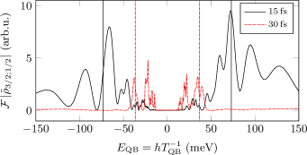
Figure 4: Fourier transform of the degree of coherence depicted in Figure 3, for the two different pulse durations; solid black line: $\tau=$15\text{\,}\mathrm{fs}$$, dot-dashed red line: $\tau=$30\text{\,}\mathrm{fs}$$. Since $\hbar\omega\equiv\eta\Delta E_{\textrm{s--o}}$ has dimension of energy, the conjugate variable has dimension of time. Here, we instead plot the peaks as a function of the quantum beat energy $E_{\textrm{QB}}$, i.e. the energy separation between neighbouring antenna transitions. The vertical lines indicate the spectral width of the driving pulse, $\delta E=\hbar\sqrt{4\ln 2}\tau^{-1}$, which for $\tau=$15\text{\,}\mathrm{fs}$$ is $\sim$73.1\text{\,}\mathrm{meV}$$ and $\sim$36.5\text{\,}\mathrm{meV}$$ for $\tau=$30\text{\,}\mathrm{fs}$$.

To further investigate the role of the Rydberg states excited via the Freeman resonances, we perform a Fourier transform of the degree of coherence along the $\eta$ axis. This analysis reveals quantum beat periods of the excited wavepacket, which constitute a fingerprint of the atomic antenna. By inverting the quantum beat periods, we instead get the energy separation between neighbouring antenna transitions, which is shown in Figure 4. As is evident from Figure 4, the very complex coherence patterns in Figure 3 is in fact due to a small number of individual antenna transitions. These transitions occur for energy separations close to the bandwidth of the driving pulse. This is not an accident: transitions at these energies reach an optimal balance between the available photon fluence (decreasing away from the carrier frequency, making the transition less likely) and the number of photons needed to be emitted/absorbed to close the spin–orbit gap, which decreases for larger energy separations (increasing the transition probability). When the pulse duration increases, the spectral bandwidth decreases. This imposes stricter requirements on which antenna transitions are in resonance with the driving field with photon energy $\hbar\omega$. It is more likely to find such transitions among the higher-lying states in the Rydberg quasi-continuum, which are more closely spaced energetically. This explains why for the longer pulse duration, we in Figure 4 observe quantum beat components of the wave packet with comparatively smaller $E_{\textrm{QB}}$, corresponding to the more tightly spaced peaks in Figure 3.

This circumstance also helps us understand why the longer pulse duration can produce larger degrees of coherence, when we might have expected the opposite; decreasing spectral bandwidth leads to narrower photoelectron peaks [35], which in turn leads to smaller energetic overlap between the ATI progressions. However, as long we are in resonance with the antenna, a longer pulse is beneficial since we can transfer population into the different pathways, while maintaining coherence. This is reminiscent of the previously studied case of weak-photon ionization of xenon [36], where longer pulse durations also led to increased ionic coherence, albeit for a simpler resonance condition.

We emphasize that, although the electron–electron interaction is crucial for the effectiveness of the antenna mechanism, the initial asymmetry is created by the laser field, which imposes the natural quantization axis on the system. The asymmetry is then transferred to the electron spin through the spin–orbit interaction (electron spins do not couple to the laser field in the dipole approximation). Finally, the electron–electron interaction provides the very efficient coupling between the Rydberg electron (the “antenna”) and the ion core. Thus, all three interactions are essential, with each playing a distinct role in the process.

IV Conclusions

We have shown that through the intermediate Rydberg state dynamics, we can introduce coherence between ionization pathways that would otherwise have opposite parity by symmetry. The coherence is sensitive to the frequency and duration of the ionizing laser pulse, and allows us to identify the effect of the Rydberg atomic antenna essentially background-free.

Appendix A Methods

We employ Hartree atomic units and implied summation/integration over indices, orbitals, momenta, and/or spins appearing on only one side of an equation.

A.1 Grid-Based Time-Dependent Configuration-Interaction Singles

The derivation of the equations of motion (EOMs), and a detailed description of the propagator are given in [14, *Carlstroem2022tdcisII]; the EOMs agree with those of Rohringer et al. [12], Greenman et al. [13], apart from the fact that spin-restriction is not imposed in the present work, i.e. we are solving the two-component Schrödinger equation.

The TD-CIS EOMs describe the time evolution of the amplitude $c_{0}$ for the Hartree–Fock (HF) reference state, and the particle orbital $\ket*{\tilde{k}}$ emanating from the occupied (time-independent) orbital $\ket{k}$. The different particle–hole channels can couple via either the laser interaction or the Coulomb interaction:

$$\mathrm{i}\partial_{t}c_{0} ={\matrixelement*{k}{\hat{V}_{L}}{\tilde{k}}},$$ (4)

$$\mathrm{i}\partial_{t}\ket*{\tilde{k}} =(-\epsilon_{k}+{\hat{f}})\ket*{\tilde{k}}+{c_{0}\hat{V}_{L}\ket{k}}-{\matrixelement{l}{\hat{V}_{L}}{k}}\ket*{\tilde{l}}$$

$$\hphantom{=}-{(\hat{J}_{lk}-\hat{K}_{lk})\ket*{\tilde{l}}}-\lambda_{\tilde{k}i}\ket{i},$$

where $\epsilon_{k}$ is the field-free energy of the occupied orbital $\ket{k}$, $(\hat{f}-\hat{V}_{L}-\epsilon_{k})\ket{k}=0$, the Fock operator is defined as $\hat{f}\overset{\textrm{\tiny def}}{=}\hat{h}+\hat{J}_{ii}-\hat{K}_{ii}$, with the one-body Hamiltonian containing the interaction with the external laser field, $\hat{h}\overset{\textrm{\tiny def}}{=}p^{2}/2+\hat{V}_{C}(\bm{r})+\hat{V}_{L}$, $\hat{V}_{L}\overset{\textrm{\tiny def}}{=}\bm{F}(t)\cdot\bm{r}$, and the direct and exchange interaction potentials are given by their action on an orbital

$$\hat{J}_{cd}\ket{e} \overset{\textrm{\tiny def}}{=}\chi_{e}(\varsigma_{1})\int\frac{\mathrm{d}\varsigma_{2}}{\left|\bm{r}_{1}-\bm{r}_{2}\right|}\chi_{c}^{*}(\varsigma_{2})\chi_{d}(\varsigma_{2}),$$

$$\hat{K}_{cd}\ket{e} \overset{\textrm{\tiny def}}{=}\chi_{d}(\varsigma_{1})\int\frac{\mathrm{d}\varsigma_{2}}{\left|\bm{r}_{1}-\bm{r}_{2}\right|}\chi_{c}^{*}(\varsigma_{2})\chi_{e}(\varsigma_{2})\equiv\hat{J}_{ce}\ket{d},$$

where $\varsigma_{1,2}$ refer to both spatial and spin coordinates of the orbitals. As we consider atoms in the present work, the particle orbitals $\ket*{\tilde{k}}\ket*{\tilde{l}}...$ are conveniently expanded in a tensor product basis formed from spinor spherical harmonics [i.e. $n\ell jm_{j}$; see §7.2 of 37] and finite-differences for the radial dimension [38, 39]. Finally, the Lagrange multiplier $\lambda_{\tilde{k}i}$ ensures that $\ket*{\tilde{k}}$ at all times remains orthogonal to the occupied orbital $\ket{i}$.

Because we are working in the dipole approximation, $\hat{V}_{L}$ includes $\mathrm{E}_{1}$ transitions only. As discussed in the main text, ${\mathrm{5p}}^{-1}_{3/2}$ and ${\mathrm{5p}}^{-1}_{1/2}$ have the same parity, which means $\matrixelement*{{\mathrm{5p}}^{-1}_{3/2}}{\hat{V}_{L}}{{\mathrm{5p}}^{-1}_{1/2}}=0$. However, even if the dipole-forbidden ($\mathrm{E}_{2}$ and $\mathrm{M}_{1}$) transitions between ${\mathrm{5p}}^{-1}_{3/2}$ and ${\mathrm{5p}}^{-1}_{1/2}$ were to be included, they would be so minuscule [40, 41] that the resulting coherence would be $\sim${10}^{-7}$$ to $\sim${10}^{-9}$$. Instead, in our simulations we find coherence $\sim${10}^{-2}$$ for all $\eta\sim 1$.

A.2 Atomic Structure and Pulse Parameters

The EOMs (4) as formulated would yield the same result as a one-component calculation, i.e. there would be no effect due to the spin of the electrons. To implement spin–orbit coupling (as well as corrections due to scalar-relativistic effects), and at the same time reducing the number of electrons we need to treat in the calculation, we replace the scalar potential $\hat{V}_{C}$ by the relativistic effective core potential (RECP) of Peterson et al. [16], which models the nucleus and the $\mathrm{1s}$–$\mathrm{3d}$ electrons according to

$$\hat{V}_{\textrm{PP}}(\bm{r})=-\frac{Q}{r}+B_{\ell j}^{k}\exp(-\beta_{\ell j}^{k}r^{2})\hat{P}_{\ell j},$$

where $Q=26$ is the residual charge, $\hat{P}_{\ell j}$ is a projector on the spin–angular symmetry $\ell j$, and $B_{\ell j}^{k}$ and $\beta_{\ell j}^{k}$ are numeric coefficients found by fitting to multiconfigurational Dirac–Fock all-electron calculations of the excited spectrum. For a thorough introduction to RECPs, see e.g. the review by Dolg and Cao [42].

The radial grid consists of 527 points extending to $90.4\text{\,}\mathrm{B}\mathrm{o}\mathrm{h}\mathrm{r}$ with the spacing smoothly varying according to [39]:

$$r_{j}=r_{j-1}+\rho_{\textrm{min}}+(1-\mathrm{e}^{-\alpha r_{j-1}})(\rho_{\textrm{max}}-\rho_{\textrm{min}}),$$

with $r_{1}=\rho_{\textrm{min}}/2$, $\rho_{\textrm{min}}=$0.1154\text{\,}\mathrm{B}\mathrm{o}\mathrm{h}\mathrm{r}$$, $\rho_{\textrm{max}}=$0.1768\text{\,}\mathrm{B}\mathrm{o}\mathrm{h}\mathrm{r}$$, and $\alpha=0.3$. The spin–angular grid is limited to $\Delta m_{j}=0$ since we only consider linearly polarized light. For pulses of duration $15\text{\,}\mathrm{fs}$ we use $\ell_{\textrm{max}}=40$, and for $30\text{\,}\mathrm{fs}$ $\ell_{\textrm{max}}=60$.

Finally, since the calculation is performed in a finite computational domain, we use Manolopoulos’ [43] transmission-free complex-absorbing potential covering the last $12.57\text{\,}\mathrm{B}\mathrm{o}\mathrm{h}\mathrm{r}$ at the far end of the box, with a design parameter $\delta\approx 0.21$; this choice gives $<$1\text{\,}\mathrm{\char 37\relax}$$ reflection for photoelectrons with kinetic energies above $3.4\text{\,}\mathrm{eV}$ ($\iff k_{\textrm{min}}=$0.5\text{\,}\mathrm{a}\mathrm{u}$$).

Table 2: Calculated ionization potentials of the 5{s,p} electrons of xenon, compared with their experimental values. The corresponding Keldysh parameters, for the range of photon energies used, indicate that ionization is in a regime intermediate between the multi-photon and tunneling limits.

Hole	$I_{\mathrm{p}}$ ($\mathrm{eV}$)	Exp. [34] ($\mathrm{eV}$)	$\Delta$ ($\mathrm{eV}$)	Keldysh $\gamma$
${\mathrm{5s}}^{-1}_{1/2}$	$27.927$	$23.397$	$4.530$	$1.84$–$2.25$
${\mathrm{5p}}^{-1}_{1/2}$	$13.483$	$13.436$	$0.047$	$1.28$–$1.73$
${\mathrm{5p}}^{-1}_{3/2}$	$12.026$	$12.130$	$-0.104$	$1.21$–$1.63$

With these grid parameters, the ionization potentials for the xenon model (only 5s and 5p orbitals are allowed to ionize) are given in Table 2; the calculated spin–orbit splitting is approximately $\Delta E_{\textrm{s--o}}\approx$1.46\text{\,}\mathrm{eV}$$. The deviation from the experimental ionization potential is much larger for ${\mathrm{5s}}^{-1}_{1/2}$; this is to be expected at the CIS level of theory, where the ion is not allowed to relax. This is however immaterial for the present work, since its ionization fraction is negligible.

The driving field frequency is scanned across the range $\eta\overset{\textrm{\tiny def}}{=}\hbar\omega/\Delta E_{\textrm{s--o}}\in[0.85,1.15]$ $\implies$ $\hbar\omega$ $=$ $1.24\text{\,}\mathrm{eV}1.68\text{\,}\mathrm{eV}$, and its intensity $I_{0}=$4.4\text{\times}{10}^{13}\text{\,}\mathrm{W}\text{\,}{\mathrm{cm}}^{-2}$$ $\implies$ $U_{\mathrm{p}}$ $=$ $4.12\text{\,}\mathrm{eV}2.25\text{\,}\mathrm{eV}$ is chosen such that the ionization remains at the level of a few percent. The pulse duration is $15\text{\,}\mathrm{fs}$ or $30\text{\,}\mathrm{fs}$, and the pulse shape is a smoothly truncated Gaussian [44], with $t_{1}=$25.5\text{\,}\mathrm{fs}$$, $t_{2}=$38.2\text{\,}\mathrm{fs}$$ and $t_{1}=$51.0\text{\,}\mathrm{fs}$$, $t_{2}=$76.4\text{\,}\mathrm{fs}$$, respectively. The time propagator is second-order accurate, and 2000 steps per carrier cycle are taken, which yields a time step $\tau$ varying from $1.67\text{\,}\mathrm{as}1.23\text{\,}\mathrm{as}$, for the range of values of $\eta$ quoted above.

A.3 Photoelectron Spectra and Ion Coherences

Photoelectron spectra are computed using a multichannel extension [14, *Carlstroem2022tdcisII] of the tSURFF [18, 19, 20, 21, 22] and iSURFV [23] techniques, yielding the familiar close-coupling [45] decomposition of the wavefunction, resolved on final ion state $I$, and photoelectron momentum $\bm{k}$ and spin $\sigma_{z}$ (it is assumed that the ion and photoelectron sufficiently separated, such that antisymmetrization can be safely omitted):

$$\ket{\Psi}=c_{I\bm{k}\sigma_{z}}\ket{I}\ket{\bm{k}\sigma_{z}}.$$

From this long-range Ansatz, we can form the density matrix of the total system

$$\hat{\rho}_{I\bm{k}^{\prime}\sigma_{z}^{\prime};J\bm{k}^{\prime\prime}\sigma_{z}^{\prime\prime}}\overset{\textrm{\tiny def}}{=}\outerproduct{\Psi}{\Psi}=c_{I\bm{k}^{\prime}\sigma_{z}^{\prime}}\ket{\bm{k}^{\prime}\sigma_{z}^{\prime}}\outerproduct{I}{J}\bra{\bm{k}^{\prime\prime}\sigma_{z}^{\prime\prime}}c_{J\bm{k}^{\prime\prime}\sigma_{z}^{\prime\prime}}^{*},$$

and by subsequently tracing out the photoelectron, the reduced density matrix, expressing the coherence between ion states

$$\rho_{IJ}=\bra{\bm{k}\sigma_{z}}\matrixelement{I}{\hat{\rho}}{J}\ket{\bm{k}\sigma_{z}}=c_{I\bm{k}\sigma_{z}}c_{J\bm{k}\sigma_{z}}^{*},$$

(the population for the ion state $I$ is $\rho_{I}\equiv\rho_{II}$). These quantities are used to compute the degree of coherence as shown in Eq. (1).

Appendix B Confirming the Atomic Antenna

Below, we will discuss various aspects of the atomic antenna [7], and avenues we have pursued to confirm that this proposed mechanism is indeed responsible for the observed symmetry breaking and non-vanishing coherence.

B.1 Influence of Depletion

Since the degree of coherence is on the order of a few percent, similar to the level of ionization for the intensity chosen, an alternative explanation could be depletion-induced residual coherence. This would be a memory effect, similar to hole-burning, deviating from the cycle-to-cycle adiabaticity and breaking the time-translation symmetry [46, 47]. To rule out this possibility, we artificially prevented the depletion of the ground state by renormalizing the ground state amplitude after every time step, which did not appreciably change the final coherence.

B.2 Dynamical Effects due to the Envelope

We also investigated whether the dynamical AC Stark shift of the Rydberg states due to the envelope of the laser field had any influence on the coherence. Substituting the Gaussian envelope by a flattop pulse, removes most of the dynamical shifts, leaving only a constant AC Stark shift. The degree of coherence was mostly unaffected by this change, only increasing by a few percent.

B.3 Removing one Rydberg State

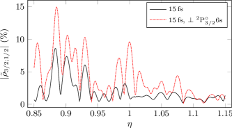
Figure 5: Effect on the degree of coherence by removing ${\mathrm{5p}}^{-1}_{3/2}\;\mathrm{6s}$ from the calculation, see Equation (5); black, solid line, the degree of coherence for a $15\text{\,}\mathrm{fs}$ pulse (same as seen in Figure 3 of the main article), and red, dot-dashed line, the degree of coherence for the same pulse, but with ${\mathrm{5p}}^{-1}_{3/2}\;\mathrm{6s}$ projected out.

We next consider the effects of specific Rydberg states; we begin by confirming that the Rydberg states, populated via frustrated tunnelling, are important in the formation of the antenna. To test this hypothesis we repeated the calculation, while preventing the ${\mathrm{5p}}^{-1}_{3/2}\;\mathrm{6s}$ state from being intermediately excited via the laser interaction. The propagator $\mathcal{U}_{L}$ for the laser interaction $\hat{V}_{L}$ is replaced according to

$$\mathcal{U}_{L}\to\hat{P}\mathcal{U}_{L}\hat{P}+\hat{Q},$$ (5)

where $\hat{Q}$ is the projector onto the ${\mathrm{5p}}^{-1}_{3/2}\;\mathrm{6s}$ state and $\hat{P}\equiv\hat{\mathbf{1}}-\hat{Q}$ is the projector onto the orthogonal complement. In this way, the ${\mathrm{5p}}^{-1}_{3/2}\;\mathrm{6s}$ state is still present in the calculation, but it will not be coupled via the laser field; we can do this since in the length gauge, the field-free excited state remains a good approximation to the time-dependent eigenstate. The state chosen has $\sim$0.979$$ contribution from the ${\mathrm{5p}}^{-1}_{3/2}$ manifold, $\sim$1.95\text{\times}{10}^{-2}$$ contribution from ${\mathrm{5p}}^{-1}_{1/2}$, and $\sim$1.82\text{\times}{10}^{-3}$$ contribution from ${\mathrm{5s}}^{-1}_{1/2}$ through configuration interaction, which makes it a likely candidate for the antenna mechanism.

As we see in Figure 5, the degree of coherence is strongly altered by the removal of ${\mathrm{5p}}^{-1}_{3/2}\;\mathrm{6s}$, confirming the importance of the Rydberg states in the formation of the antenna. The exact influence of individual states on the antenna efficiency and the final coherence is a topic for future investigations.

B.4 Antenna Transition Strength

We now would like to investigate whether there is a correlation between the transitions in the Rydberg manifold that constitute our antenna, and the observed variation of the degree of coherence $\tilde{\rho}_{3/2;1/2}$ with the photon energy. The weight of the antenna transition between states $a$ and $b$ is estimated as

$$w_{ab}=\left|z_{ab}\right|^{2}[\min(|c^{(a)}_{3/2}|^{2},|c^{(a)}_{1/2}|^{2})+\min(|c^{(b)}_{3/2}|^{2},|c^{(b)}_{1/2}|^{2})],$$ (6)

where $c^{(s)}_{J}$ is the complex amplitude of state $s$ in channel $J$. Diagonalizing the field-free Hamiltonian [(4) with $\hat{V}_{L}=0$], we obtain the first 150 excited states, and compute (6) for all dipole-allowed transitions. Those that fall within the energy interval we consider, are shown as a stick spectrum in Figure 6, alongside the degree of coherence. By convoluting the stick spectrum with a Lorentzian

$$\Lambda(\omega)=\frac{1}{1+x^{2}},\quad x=\frac{2\omega}{\Gamma},$$ (7)

where $\Gamma$ is the full width at half maximum, a continuous distribution is acquired; we use $\Gamma=$5\text{\times}{10}^{-4}\text{\,}\mathrm{Ha}$$, $h/\Gamma\sim$48\text{\,}\mathrm{fs}$$.

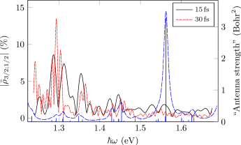
Figure 6: Antenna transitions: The left ordinate corresponds to the degree of coherence for $15\text{\,}\mathrm{fs}$ and $30\text{\,}\mathrm{fs}$ are shown in solid black and dot-dashed red lines, respectively. The right ordinate corresponds to the antenna strengths, computed using (6) and shown as sticks, and convoluted with a Lorentzian spectral shape (7), shown as the dashed blue line.

The similarity of the convoluted spectrum with the degree of coherence is very suggestive, apart from the very strong peak at $\sim$1.56\text{\,}\mathrm{eV}$$, which is due to a very strong dipole moment for that transition. Exact agreement can, however, not be expected for a variety of reasons. Equation (6) considers dipole transitions between field-free states, i.e. disregarding any Stark shifts in the strong field, which means the transitions might not occur at the positions indicated. More important, though, is the fact that we completely disregard the relative populations of the constituent states, which, when prepared through frustrated tunnelling depend strongly on the laser parameters [28].

B.5 Antenna Size

We now wish to estimate the effective size of the antenna structure, and relate that to the driving wavelength. In classical electromagnetic theory, a dipole antenna will exhibit the largest gain if the length is $5\lambda/4$; $\lambda/2$ is also very common. Naturally, electron excursions on that scale would far exceed the applicability of the dipole approximation, however, this gives a clear motivation for why large electronic structures are desirable to efficiently couple the external electric field into the atom.

An excited state can in the CIS Ansatz be written as

$$\sum_{k}\tilde{\Phi}_{k},$$

with the particle orbital $\ket*{\tilde{k}}$ containing all information about the electron in the channel associated with excitation/ionization from the occupied orbital $\ket{k}$. We estimate the size of the state as

$$s_{1}\overset{\textrm{\tiny def}}{=}\sqrt{\sum_{k}\matrixelement*{\tilde{k}}{r^{2}}{\tilde{k}}};\quad s_{2}\overset{\textrm{\tiny def}}{=}\sum_{k}\sqrt{\matrixelement*{\tilde{k}}{r^{2}}{\tilde{k}}}.$$

The size of the antenna is then estimated as the geometric mean of the sizes of the two states:

$$\sqrt{s(a)s(b)}$$

For the transitions in Figure 6, the estimates fall in the range $1\text{\,}\mathrm{nm}3\text{\,}\mathrm{nm}$, and with a driving wavelength of $\lambda\sim$900\text{\,}\mathrm{nm}$$, this corresponds to $\frac{\lambda}{900}-\frac{\lambda}{300}$ antenna structures. This is of course far from the optimum $\frac{5\lambda}{4}$, but a lot better than what could be expected from the orbitals of the ground state; $\mathrm{5\{s,p\}}$ have a size of $\sim$0.1\text{\,}\mathrm{nm}$$ which would yield a $\frac{\lambda}{9000}$ antenna.

B.6 Coherence due to Single Rydberg States

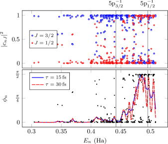
Figure 7: Rydberg states channel decomposition for the 500 first excited states of xenon; the top panel shows the populations of state $n$ in ${\mathrm{5p}}^{-1}_{3/2}$ (blue circles) and ${\mathrm{5p}}^{-1}_{1/2}$ (red diamonds), respectively, as a function of its excitation energy $E_{n}$. ${\mathrm{5s}}^{-1}_{1/2}$ contributions are negligible for these states. The vertical lines indicate the positions of the ionization thresholds. The bottom panel shows the mixing angle $\phi_{n}\overset{\textrm{\tiny def}}{=}\arctan(\left|c_{n;1/2}\right|/\left|c_{n;3/2}\right|)$; $\phi_{n}=0$ indicates a state purely in ${\mathrm{5p}}^{-1}_{3/2}$, $\phi_{n}=\pi/2$ indicates a state purely in ${\mathrm{5p}}^{-1}_{1/2}$, and $\phi_{n}=\pi/4$ indicates an even mixture. The lines show the average mixing angle as a function of excitation energy, when convolving with a Gaussian corresponding to $15\text{\,}\mathrm{fs}$ duration (solid blue), and $30\text{\,}\mathrm{fs}$ duration (dashed red).

Through resonant excitation, it is possible to generate high degrees of coherence, since some Rydberg states have large mixing fractions in ${\mathrm{5p}}^{-1}_{3/2}$ and ${\mathrm{5p}}^{-1}_{1/2}$. If an excited state has equal amplitudes in the two channels, tracing out the excited electron would yield an ionic superposition with $100\text{\,}\mathrm{\char 37\relax}$ degree of coherence. By choosing the excited state judiciously, we can thus achieve any desired degree of coherence from $0\text{\,}\mathrm{\char 37\relax}100\text{\,}\mathrm{\char 37\relax}$. In Figure 7, we show the mixing coefficients of the first 500 excited states of xenon. Below the ${\mathrm{5p}}^{-1}_{3/2}$ threshold, the $J=3/2$ component is dominant, with only a few states achieving large fractions of $J=1/2$. Between the thresholds, the $J=1/2$ component becomes more important. It is precisely the latter states that Dill [32] considered, studying the importance of the spin–orbit interaction in photoionization.

Can resonant excitation of an intermediate state with high mixing between ${\mathrm{5p}}^{-1}_{3/2}$ and ${\mathrm{5p}}^{-1}_{1/2}$ explain our observed degree of coherence in Figure 3? Let us first consider weak-field ionization, where we first through one-photon absorption populate the intermediate state with energy $E_{n}$, which we may write as

$$\ket{\Psi_{n}}=\mathcal{A}(c_{I}\ket{I}\ket{n_{I}}+c_{J}\ket{J}\ket{n_{J}}),$$ (8)

where $\mathcal{A}$ is the antisymmetrization operator. Subsequent single-photon ionization will lead to a final state on the form (2). However, even if $c_{I}$ and $c_{J}$ in (8) are both significant, $w=\innerproduct*{\chi_{I}}{\chi_{J}}$ in (2) will still vanish due to energy conservation; the photoelectron peaks will appear at $W_{k}=\omega-(I_{\mathrm{p},{I}}-E_{n})$ and $W_{k}=\omega-(I_{\mathrm{p},{J}}-E_{n})$, respectively. This is not the case in the process considered by Dill [32], since the final state involves only one ion channel, namely ${\mathrm{5p}}^{-1}_{3/2}$, which is populated through direct ionization, as well as autoionization of the intermediately excited states below the ${\mathrm{5p}}^{-1}_{1/2}$ threshold. Thus energy conservation is automatically fulfilled.

We next consider strong-field ionization. In this case, it is difficult to address a single state. Instead, we access the average coherence of the state manifold, which remains low; see the average mixing angle in the lower panel of Figure 7. Furthermore, subsequent ionization and generation of ATI progressions would still face the same predicament as stated earlier: for $\eta\sim 1$, the photoelectron peaks of similar kinetic energy would result from absorption of a different number of photons, and thus by parity, their overlap would vanish. The atomic antenna, which repeatedly accesses parts of the excited spectrum with high mixing fractions, allows us to amplify this small, average mixing coefficient.

References

- Wragg et al. [2019] J. Wragg, D. D. A. Clarke, G. S. J. Armstrong, A. C. Brown, C. P. Ballance, and H. W. van der Hart, Resolving ultrafast spin–orbit dynamics in heavy many-electron atoms, Physical Review Letters 123, 163001 (2019).
- Kübel et al. [2019] M. Kübel, Z. Dube, A. Y. Naumov, D. M. Villeneuve, P. B. Corkum, and A. Staudte, Spatiotemporal imaging of valence electron motion, Nature Communications 10, 1042 (2019).
- Goulielmakis et al. [2010] E. Goulielmakis, Z.-H. Loh, A. Wirth, R. Santra, N. Rohringer, V. S. Yakovlev, S. Zherebtsov, T. Pfeifer, A. M. Azzeer, M. F. Kling, S. R. Leone, and F. Krausz, Real-time observation of valence electron motion, Nature 466, 739 (2010).
- Hartung et al. [2016] A. Hartung, F. Morales, M. Kunitski, K. Henrichs, A. Laucke, M. Richter, T. Jahnke, A. Kalinin, M. Schöffler, L. P. H. Schmidt, and et al., Electron spin polarization in strong-field ionization of xenon atoms, Nature Photonics 10, 526 (2016).
- Barth and Smirnova [2013] I. Barth and O. Smirnova, Spin-polarized electrons produced by strong-field ionization, Physical Review A 88, 013401 (2013).
- Barth and Smirnova [2014] I. Barth and O. Smirnova, Hole dynamics and spin currents after ionization in strong circularly polarized laser fields, Journal of Physics B: Atomic, Molecular and Optical Physics 47, 204020 (2014).
- Kuchiev [1987] M. Y. Kuchiev, Atomic antenna, Soviet Journal of Experimental and Theoretical Physics Letters 45, 404 (1987).
- Tzur et al. [2021] M. E. Tzur, O. Neufeld, A. Fleischer, and O. Cohen, Selection rules for breaking selection rules, New Journal of Physics 23, 103039 (2021).
- Nesbet [1955] R. K. Nesbet, Configuration interaction in orbital theories, Proceedings of the Royal Society of London. Series A. Mathematical and Physical Sciences 230, 312 (1955).
- Löwdin [1955] P.-O. Löwdin, Quantum theory of many-particle systems. I. Physical interpretations by means of density matrices, natural spin-orbitals, and convergence problems in the method of configurational interaction, Physical Review 97, 1474 (1955).
- Krause et al. [2005] P. Krause, T. Klamroth, and P. Saalfrank, Time-dependent configuration-interaction calculations of laser-pulse-driven many-electron dynamics: Controlled dipole switching in lithium cyanide, The Journal of Chemical Physics 123, 074105 (2005).
- Rohringer et al. [2006] N. Rohringer, A. Gordon, and R. Santra, Configuration-interaction-based time-dependent orbital approach for Ab Initio treatment of electronic dynamics in a strong optical laser field, Physical Review A 74, 043420 (2006).
- Greenman et al. [2010] L. Greenman, P. J. Ho, S. Pabst, E. Kamarchik, D. A. Mazziotti, and R. Santra, Implementation of the time-dependent configuration-interaction singles method for atomic strong-field processes, Physical Review A 82, 023406 (2010).
- Carlström et al. [2022a] S. Carlström, M. Spanner, and S. Patchkovskii, General time-dependent configuration-interaction singles I: The molecular case, arXiv:2204.09966 [physics.chem-ph] (2022a), accepted for publication in Physical Review A.
- Carlström et al. [2022b] S. Carlström, M. Bertolino, J. M. Dahlström, and S. Patchkovskii, General time-dependent configuration-interaction singles II: The atomic case, arXiv:2204.10534 [physics.atom-ph] (2022b), accepted for publication in Physical Review A.
- Peterson et al. [2003] K. A. Peterson, D. Figgen, E. Goll, H. Stoll, and M. Dolg, Systematically convergent basis sets with relativistic pseudopotentials. II. Small-core pseudopotentials and correlation consistent basis sets for the post-d group 16–18 elements, The Journal of Chemical Physics 119, 11113 (2003).
- Zapata et al. [2022] F. Zapata, J. Vinbladh, A. Ljungdahl, E. Lindroth, and J. M. Dahlström, Relativistic time-dependent configuration-interaction singles method, Physical Review A 105, 012802 (2022).
- Ermolaev et al. [1999] A. M. Ermolaev, I. V. Puzynin, A. V. Selin, and S. I. Vinitsky, Integral boundary conditions for the time-dependent Schrödinger equation: Atom in a laser field, Physical Review A 60, 4831 (1999).
- Ermolaev and Selin [2000] A. M. Ermolaev and A. V. Selin, Integral boundary conditions for the time-dependent Schrödinger equation: Superposition of the laser field and a long-range atomic potential, Physical Review A 62, 015401 (2000).
- Serov et al. [2001] V. V. Serov, V. L. Derbov, B. B. Joulakian, and S. I. Vinitsky, Wave-packet evolution approach to ionization of the hydrogen molecular ion by fast electrons, Physical Review A 63, 062711 (2001).
- Tao and Scrinzi [2012] L. Tao and A. Scrinzi, Photo-electron momentum spectra from minimal volumes: the time-dependent surface flux method, New Journal of Physics 14, 013021 (2012).
- Scrinzi [2012] A. Scrinzi, t-SURFF: Fully Differential Two-Electron Photo-Emission Spectra, New Journal of Physics 14, 085008 (2012).
- Morales et al. [2016] F. Morales, T. Bredtmann, and S. Patchkovskii, iSURF: a family of infinite-time surface flux methods, Journal of Physics B: Atomic, Molecular and Optical Physics 49, 245001 (2016).
- Pabst et al. [2016] S. Pabst, M. Lein, and H. J. Wörner, Preparing attosecond coherences by strong-field ionization, Physical Review A 93, 023412 (2016).
- Ruberti et al. [2018] M. Ruberti, P. Decleva, and V. Averbukh, Full Ab Initio many-electron simulation of attosecond molecular pump-probe spectroscopy, Journal of Chemical Theory and Computation 14, 4991 (2018).
- Ruberti [2019] M. Ruberti, Onset of ionic coherence and ultrafast charge dynamics in attosecond molecular ionisation, Physical Chemistry Chemical Physics 21, 17584 (2019).
- Ruberti [2021] M. Ruberti, Quantum electronic coherences by attosecond transient absorption spectroscopy: Ab Initio B-spline RCS-ADC study, Faraday Discussions 228, 286 (2021).
- Nubbemeyer et al. [2008] T. Nubbemeyer, K. Gorling, A. Saenz, U. Eichmann, and W. Sandner, Strong-field tunneling without ionization, Physical Review Letters 101, 233001 (2008).
- Eichmann et al. [2009] U. Eichmann, T. Nubbemeyer, H. Rottke, and W. Sandner, Acceleration of neutral atoms in strong short-pulse laser fields, Nature 461, 1261 (2009).
- Zimmermann et al. [2017] H. Zimmermann, S. Patchkovskii, M. Ivanov, and U. Eichmann, Unified time and frequency picture of ultrafast atomic excitation in strong laser fields, Physical Review Letters 118, 013003 (2017).
- Freeman et al. [1987] R. R. Freeman, P. H. Bucksbaum, H. Milchberg, S. Darack, D. Schumacher, and M. E. Geusic, Above-threshold ionization with subpicosecond laser pulses, Physical Review Letters 59, 1092 (1987).
- Dill [1973] D. Dill, Resonances in photoelectron angular distributions, Physical Review A 7, 1976 (1973).
- Samson and Gardner [1973] J. A. R. Samson and J. L. Gardner, Resonances in the angular distribution of xenon photoelectrons, Physical Review Letters 31, 1327 (1973).
- Saloman [2004] E. B. Saloman, Energy levels and observed spectral lines of xenon, Xe I through Xe LIV, Journal of Physical and Chemical Reference Data 33, 765 (2004).
- Petite et al. [1987] G. Petite, P. Agostini, and F. Yergeau, Intensity, pulse width, and polarization dependence of above-threshold-ionization electron spectra, Journal of the Optical Society of America B 4, 765 (1987).
- Carlström et al. [2018] S. Carlström, J. Mauritsson, K. J. Schafer, A. L’Huillier, and M. Gisselbrecht, Quantum coherence in photo-ionisation with tailored XUV pulses, Journal of Physics B: Atomic, Molecular and Optical Physics 51, 015201 (2018).
- Varshalovich [1988] D. A. Varshalovich, Quantum Theory of Angular Momentum: Irreducible Tensors, Spherical Harmonics, Vector Coupling Coefficients, 3nj Symbols (World Scientific Pub, Singapore Teaneck, NJ, USA, 1988).
- Adler and Piran [1984] S. L. Adler and T. Piran, Relaxation methods for gauge field equilibrium equations, Reviews of Modern Physics 56, 1 (1984).
- Krause and Schafer [1999] J. L. Krause and K. J. Schafer, Control of THz emission from Stark wave packets, The Journal of Physical Chemistry A 103, 10118 (1999).
- Garstang [1964] R. Garstang, Transition probabilities of forbidden lines, Journal of Research of the National Bureau of Standards Section A: Physics and Chemistry 68A, 61 (1964).
- Nandy and Sahoo [2015] D. K. Nandy and B. K. Sahoo, Forbidden transition properties in the ground-state configurations of singly ionized noble gas atoms for stellar and interstellar media, Monthly Notices of the Royal Astronomical Society 450, 1012 (2015).
- Dolg and Cao [2011] M. Dolg and X. Cao, Relativistic pseudopotentials: Their development and scope of applications, Chemical Reviews 112, 403 (2011).
- Manolopoulos [2002] D. E. Manolopoulos, Derivation and reflection properties of a transmission-free absorbing potential, J. Chem. Phys. 117, 9552 (2002).
- Patchkovskii and Muller [2016] S. Patchkovskii and H. Muller, Simple, accurate, and efficient implementation of 1-electron atomic time-dependent Schrödinger equation in spherical coordinates, Computer Physics Communications 199, 153 (2016).
- Fritsch and Lin [1991] W. Fritsch and C.-D. Lin, The semiclassical close-coupling description of atomic collisions: Recent developments and results, Physics Reports 202, 1 (1991).
- Jankowiak et al. [1993] R. Jankowiak, J. M. Hayes, and G. J. Small, Spectral hole-burning spectroscopy in amorphous molecular solids and proteins, Chemical Reviews 93, 1471 (1993).
- Goll et al. [2006] E. Goll, G. Wunner, and A. Saenz, Formation of ground-state vibrational wave packets in intense ultrashort laser pulses, Physical Review Letters 97, 103003 (2006).