A Babcock-Leighton-type Solar Dynamo Operating in the Bulk of the Convection Zone

Abstract

The toroidal magnetic field is assumed to be generated in the tachocline in most Babcock-Leighton (BL)-type solar dynamo models, in which the poloidal field is produced by the emergence and subsequent dispersal of sunspot groups. However, magnetic activity of fully convective stars and MHD simulations of global stellar convection have recently raised serious doubts regarding the importance of the tachocline in the generation of the toroidal field. In this study, we aim to develop a new BL-type dynamo model, in which the dynamo operates mainly within the bulk of the convection zone. Our 2D model includes the effect of solar-like differential rotation, one-cell meridional flow, near-surface radial pumping, strong turbulent diffusion, BL-type poloidal source, and nonlinear back-reaction of the magnetic field on its source with a vertical outer boundary condition. The model leads to a simple dipolar configuration of the poloidal field that has the dominant latitudinal component, which is wound up by the latitudinal shear within the bulk of the convection zone to generate the toroidal flux. As a result, the tachocline plays a negligible role in the model. The model reproduces the basic properties of the solar cycle, including (a) approximately 11 yr cycle period and 18 yr extended cycle period; (b) equatorward propagation of the antisymmetric toroidal field starting from high latitudes; and (c) polar field evolution that is consistent with observations. Our model opens the possibility for a paradigm shift in understanding the solar cycle to transition from the classical flux transport dynamo.

1 Introduction

The dynamo process is responsible for the solar magnetic cycle (Hathaway, 2015). The core concept for the dynamo is that the poloidal and toroidal fields sustain each other to form periodic large-scale magnetic activity (Karak et al., 2014; Charbonneau, 2020). Differential rotation stretches the poloidal field to generate the toroidal field ($\Omega$-effect). There are several controversial mechanisms for the poloidal field regeneration ($\alpha$-effect), and the Babcock-Leighton (BL) mechanism is one of them. The essential idea behind the mechanism is that the poloidal field is generated by the observed behaviors of sunspot emergence and the subsequent evolution of the magnetic field at the surface.

The BL mechanism has received significant observational support during the last decade. In this mechanism, the sunspot group tilt angles play a key role in the construction of the poloidal source term. Dasi-Espuig et al. (2010), Kitchatinov & Olemskoy (2011), and Jiao et al. (2021) reveal that the observed sunspot group tilt angles vary systematically from cycle to cycle. The weak cycle 24 might result from abnormal tilt angles of sunspot groups in cycle 23 (Jiang et al., 2015). Furthermore, observations confirm the correlation between the polar field strength at cycle minimum and the next cycle strength implied by the BL mechanism (Schatten et al., 1978; Muñoz-Jaramillo et al., 2013; Jiang et al., 2018).

In Babcock’s original scenario (Babcock, 1961), the latitudinal differential rotation stretches the poloidal magnetic field that is represented by the global dipole to generate the toroidal field. Cameron & Schüssler (2015) find that the latitudinal differential rotation is by far the dominant generator of the net toroidal flux. The important role of the latitudinal shear in the toroidal field generation is emphasized by previous studies, such as Guerrero & de Gouveia Dal Pino (2007) and Muñoz-Jaramillo et al. (2009). However, there appears to be a long-standing consensus that the toroidal field is generated by the radial differential rotation in the tachocline; that is, the narrow radial shear layer at the bottom of the convection zone (Spiegel & Zahn, 1992).

Since their development in the 1990s, flux transport dynamo (FTD) models have emerged as a popular paradigm for the understanding of the solar cycle (Wang et al., 1991; Choudhuri et al., 1995; Durney, 1995). The BL mechanism is usually incorporated in these models, which are characterized by an important role played by the meridional flow. Moreover, the toroidal field is created in the tachocline and rises owing to magnetic buoyancy to form sunspots. The scenario for the toroidal field’s generation and emergence is supported by thin flux tube simulations (for reviews, see Fan, 2009), which can produce the proper latitudinal dependence of tilt angles with an initial field as strong as 10⁵ G (D’Silva & Choudhuri, 1993; Caligari et al., 1995). The tachocline’s significant radial shear and subadiabatic stratification may allow the magnetic fields to be amplified so tremendously before being subjected to magnetic buoyancy instabilities. These are arguments in favor of the tachocline for the toroidal field location.

However, the last few decades have seen problems with FTD models, which are directly caused by the effect of the tachocline, despite their effectiveness in producing some solar cycle features. In the polar latitudes, the tachocline has a strong radial shear, which causes the toroidal flux to prevail in polar regions (Dikpati & Charbonneau, 1999; Nandy & Choudhuri, 2002; Guerrero & Muñoz, 2004; Lemerle & Charbonneau, 2017). The concentrated toroidal flux at high latitudes causes a rather weak ratio between the toroidal field at the activity belt and polar fields (Kitchatinov & Olemskoy, 2012). There are several other problems with FTD models that are produced indirectly by the tachocline’s effect. For example, FTD models tend to generate the quadrupole-like parity (Dikpati & Gilman, 2001; Chatterjee et al., 2004; Hotta & Yokoyama, 2010) and are sensitive to the profile of the deep meridional flow, which is still controversial (for reviews, see Choudhuri, 2021).

Recent MHD simulations of global solar/stellar convection provide a new scenario for the generation of the toroidal flux. Nelson et al. (2013, 2014) and Chen et al. (2021) show that convective simulations without the tachocline spontaneously generate rope-like structures of magnetic flux that rise to the top of the simulation domain in a solar-like manner. Fan & Fang (2014), Guerrero et al. (2016), and Käpylä et al. (2017) demonstrate that solar-like large-scale magnetic fields can be produced entirely within a convection zone without extending the simulation down to the tachocline. Käpylä (2021) shows the similarity of large-scale field generation between partially and fully convective stars. Progress in MHD simulations provides an impetus to rethink the roles of the tachocline in the BL-type dynamo.

Theoretically, Spruit (2011) argues that a tachocline that has a stable stratification does not provide significant shear stresses, with which a field could be amplified. Kitchatinov & Nepomnyashchikh (2017b) argue that the radial field should be small near the base of the convection zone. The tachocline is unimportant for the dynamo, even if there is a strong radial gradient of rotation in the tachocline. See Brandenburg (2005) for other arguments against the tachocline for the toroidal field origination.

Another persuasive question on the importance of the tachocline is proposed by stellar magnetic activity. If a tachocline was really crucial for a dynamo to work, then one might expect a break in magnetic activity toward fully convective late-M dwarfs (Charbonneau, 2016). However, it appears to be continuous across the transition to full convection for most activity indicators, such as flare activity (Lin et al., 2019; Yang & Liu, 2019). In particular, the X-ray activity-rotation relationship of fully convective M-type stars is in line with partially convective stars (Wright & Drake, 2016).

All of the evidence that is listed here questions the widely accepted opinion that the toroidal field is generated by the radial shear in the tachocline. In this regard, a dynamo model operating in the bulk of the convection zone in the framework of the BL mechanism is required. Cameron & Schüssler (2017a) have taken the first step toward the new generation, in the sense that the tachocline does not play an essential role anymore, of the BL-type dynamo. They assume that the toroidal flux is generated by the radial shear in the near-surface shear layer (NSSL) and by the latitudinal shear in the bulk of the convection zone. The solar-like solutions are obtained from their quasi-1D model. However, the model cannot elaborate the radial distributions and configurations of the toroidal and poloidal fluxes, which requires the development of a 2D BL-type model.

The purpose of the present paper is to develop a 2D BL-type dynamo model, in which the toroidal field is generated in the bulk of the convection zone. The model is consistent with the key property of the standard Babcock’s scenario, which is that the latitudinal differential rotation stretches the simple dipole to generate the toroidal field.

This paper is organized as follows. The new BL-type dynamo model is described in Section 2. A reference model is presented in detail in Section 3.1. We demonstrate that our model is independent of the tachocline in Section 3.2. Comparisons with two FTD models are presented in Section 3.3. Finally, we summarize and discuss our results in Section 4.

2 MODEL

The axisymmetric large-scale magnetic field is expressed in spherical coordinates as

$$\textbf{B}(r,\theta,t)=B(r,\theta,t)\hat{\textbf{e}}_{\phi}+\nabla\times\left[A(r,\theta,t)\hat{\textbf{e}}_{\phi}\right],$$ (1)

where $B(r,\theta,t)\hat{\textbf{e}}_{\phi}$ represents the toroidal field and the curl of a magnetic vector potential in $\phi$ direction represents the poloidal field. In the kinematic framework, the large-scale flow fields are prescribed as

$$\textbf{u}(r,\theta)=r\sin\theta\Omega(r,\theta)\hat{\textbf{e}}_{\phi}+\textbf{u}_{p}(r,\theta),$$ (2)

where $\textbf{u}_{p}(r,\theta)$ represents the meridional flow, and $\Omega$ is the angular velocity. The BL-type $\alpha\Omega$ dynamo equations (for reviews, see Charbonneau, 2020) are

$$\frac{\partial A}{\partial t}+\frac{1}{s}(\textbf{u}_{p}\cdot\nabla)(sA)=\eta\left(\nabla^{2}-\frac{1}{s^{2}}\right)A+S_{BL},$$ (3)

$$\frac{\partial B}{\partial t}+\frac{1}{r}\left[\frac{\partial(ru_{r}B)}{\partial r}+\frac{\partial(u_{\theta}B)}{\partial\theta}\right]=\eta\left(\nabla^{2}-\frac{1}{s^{2}}\right)B+s(\textbf{B}_{p}\cdot\nabla\Omega)+\frac{1}{r}\frac{d\eta}{dr}\frac{\partial(rB)}{\partial r},$$ (4)

where $s=r\sin\theta$, and $\eta$ represents the turbulent diffusivity. $S_{BL}$ is the BL-type source term that describes the regeneration of the poloidal field at the solar surface. The second term on the right-hand of Equation (4) is the source term of the toroidal field, which is equal to

$$s(\textbf{B}_{r}\cdot\nabla_{r}\Omega)+s(\textbf{B}_{\theta}\cdot\nabla_{\theta}\Omega),$$ (5)

where the former term means that $B_{r}$ is stretched by the radial shear, and the latter term represents that $B_{\theta}$ is stretched by the latitudinal shear.

We specify the profiles of $\textbf{u}_{p}$, $\Omega$, $\eta$, and $S_{BL}$ in next subsections. The computational domain of our model is 0.65$R_{\odot}\leq r\leq$ $R_{\odot},0\leq\theta\leq\pi$. The outer boundary condition is that the field is vertical based on the constraint by Cameron et al. (2012). Accordingly, we use $\partial(rA)/\partial r=0$, $B=0$ at $r=R_{\odot}$. The bottom boundary matches a perfect conductor, which means that $A=0$, $\partial(rB)/\partial r=0$ at $r=0.65R_{\odot}$. At poles, $A=B=0$. Our model is computed using the code SURYA developed by A.R. Choudhuri and his colleagues (Dikpati & Choudhuri, 1994; Chatterjee et al., 2004).

2.1 BL-type source term

We define $S_{BL}$ in Equation (3) as

$$S_{BL}(r,\theta,t)=\frac{\alpha(r,\theta)\bar{B}(\theta,t)}{1+[|\bar{B}(\theta,t)|/B_{0}]^{1/4}},$$ (6)

where

$$\alpha(r,\theta)=\frac{\alpha_{0}f(\theta)}{2}\left[1+\rm erf\left(\frac{r-0.95R_{\odot}}{0.01R_{\odot}}\right)\right].$$ (7)

In the BL mechanism, the regeneration process of the poloidal field appears at the solar surface, due to the decay of tilted sunspots. Hence, the source term $S_{BL}$ represented here is confined above 0.95$R_{\odot}$. This could produce a near-surface dipole moment, which is proportional to the mean (area normalized) toroidal field over the whole convection zone,

$$\bar{B}(\theta,t)=\int_{0.7R_{\odot}}^{R_{\odot}}B(r,\theta,t)rdr/\int_{0.7R_{\odot}}^{R_{\odot}}rdr.$$ (8)

In contrast, $\bar{B}(r,\theta,t)$ is usually defined as the toroidal field in the tachocline in FTD models (e.g., Dikpati & Charbonneau, 1999; Chatterjee et al., 2004).

The latitude dependence of the source term $S_{BL}$ is

$$f(\theta)=\cos\theta\sin^{n}\theta,$$ (9)

where $\cos\theta$ reflects the latitude dependence of the tilt angles caused by the Coriolis force. Parameter $n$ controls the emergence latitude of the toroidal field. Because the buoyancy process of the toroidal field is still an open question, we treat $n$ as a free parameter, which is specified based on the condition that the results of our model fit the observations.

Generally, in a nonlinear dynamo model, a limit cycle (periodic solution) emerges from a supercritical Hopf bifurcation when the dynamo number exceeds its critical value (Tobias et al., 1995; Cameron & Schüssler, 2017b). As an amplitude limit mechanism, the nonlinear algebraic $\alpha$ quenching term $\alpha/[1+(\bar{B}/B_{0})^{2}]$ is widely used. This constrains the magnetic fields not to exceed the equipartition field $B_{0}$. However, when we consider this term in our model, the Hopf bifurcation tends to be subcritical, in which condition the saturation magnetic fields will largely exceed $B_{0}$. To achieve our desired quenching effect, we find that the quenching form needs to be $\alpha/[1+(|\bar{B}|/B_{0})^{1/4}]$. We chose the equipartition field 10⁴ G for $B_{0}$, and the units of magnetic fields in all solutions are the same as $B_{0}$. Besides the pure BL $\alpha$-effect concentrated near the solar surface presented above, we do not include any other $\alpha$-terms in our model.

2.2 Differential rotation

We use an analytical profile of the angular velocity close to helioseismic results (Schou et al., 1998). The profile is given by

$$\Omega(r,\theta)=\Omega_{RZ}+(\Omega_{CZ}-\Omega_{RZ})\Omega_{1},$$ (10)

$$\Omega_{1}=\frac{1}{2}\left[1+\rm erf\left(\frac{r-0.7R_{\odot}}{0.04R_{\odot}}\right)\right],$$ (11)

where $\Omega_{RZ}/{2\pi}=432.8$ nHz, $\Omega_{CZ}/2\pi=470.308-62.79\cos^{2}(\theta)-67.87\cos^{4}(\theta)-16.808(r-0.95$$R_{\odot})/0.05$R_⊙ nHz for $r>0.95$$R_{\odot}$, and $\Omega_{CZ}/2\pi=470.308-62.79\cos^{2}(\theta)-67.87\cos^{4}(\theta)$ nHz for $r\leq 0.95$$R_{\odot}$.

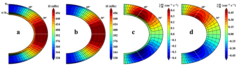
Figure 1: Contours of angular velocity profiles. (a) Angular velocity $\Omega$ of the reference model. (b) Angular velocity $\Omega$ with artificially shutting of the radial shear in the tachocline used in Section 3.2.2. (c) Latitudinal gradient of the angular velocity presented in (a). (d) Latitudinal gradient of the angular velocity presented in (b).

The distribution of $\Omega(r,\theta)$ generated by the above expression is shown in Figure 1(a). The radial shear concentrates in the tachocline and the NSSL, while the latitudinal shear concentrates in the bulk of the convection zone. To evaluate the role of the radial shear in the tachocline in Section 3.2, we set $\Omega_{1}=1$ to obtain the profile that is shown in Figure 1(b), which contains no radial shear in the tachocline. Figures 1(c) and (d) show the distributions of $(1/r)(\partial\Omega/\partial\theta)$ for the rotation profiles shown in Figures 1(a) and (b), respectively. They show the strong latitudinal shear in the bulk of the convection zone. The maximum value of $(1/r)(\partial\Omega/\partial\theta)$ appears at about 55^∘ latitude and the value of $(1/r)(\partial\Omega/\partial\theta)$ decreases with depth. Note that when the radial shear is removed, the latitudinal shear is stronger than that with the radial shear in the tachocline, especially at the base of the convection zone.

2.3 Meridional flow

We define the stream function $\psi$ that satisfies the equation,

$$\psi r\sin\theta=\psi_{0}(r-R_{p})\sin\left[\frac{\pi(r-R_{p})}{R_{\odot}-R_{p}}\right](1-e^{-\beta_{1}\theta^{\varepsilon}})[1-e^{\beta_{2}(\theta-\pi/2)}]e^{-[(r-r_{0})/\Gamma]^{2}}\sin\theta,$$ (12)

where $\beta_{1}=1.5,\beta_{2}=1.3,\varepsilon=2.0000001,r_{0}=(R_{\odot}-R_{b})/3.5,\Gamma=3.47\times 10^{8}m$ and $R_{p}=0.7R_{\odot}$. According to $\rho\textbf{u}_{p}=\nabla\times[\psi(r,\theta)]\hat{\textbf{e}}_{\phi}$, where $\rho=C(R_{\odot}/r-0.95)^{3/2}$, the profile of the meridional flow $\textbf{u}_{p}$ could be derived. By setting $\psi_{0}/C$ = 33.4 m s^-1, the amplitude of the surface velocity reaches a maximum of 20 m s^-1 at 45^∘. The inner return flow decreases to zero at $r$ = 0.7$R_{\odot}$. This profile is similar to Equation (5) of Karak & Cameron (2016), except that we add a term $\sin\theta$ in Equation (12) to decrease the flow speed near the poles.

The typical amplitudes of 10 - 20 m s^-1 for the surface poleward flow have been confirmed by several measurements (Hathaway & Rightmire, 2010; Ulrich, 2010; Basu & Antia, 2010) but there is no consensus on the inner flow (Zhao et al., 2013; Schad et al., 2013; Rajaguru & Antia, 2015; Gizon et al., 2020). The meridional flow used in our model is similar to the helioseismic results of Jackiewicz et al. (2015) in terms of the return flow starting in shallower layers.

The distributions of $u_{\theta}$ and $u_{r}$ in the meridional plane are shown in Figures 2(a) and (b), respectively. Figure 2(c) shows the radial variations of $u_{\theta}$ at 45^∘ latitudes and $u_{r}$ at 60^∘ latitudes. The return flow starts from 0.86$R_{\odot}$ and the average value of $u_{\theta}R_{\odot}/r$ is 1.6 m s^-1 in the range 0.7-0.86$R_{\odot}$ where the toroidal flux resides.

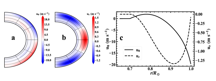
Figure 2: Meridional flow of the reference model. (a) Latitudinal component, $u_{\theta}$. (b) Radial component, $u_{r}$. (c) Radial variations of $u_{\theta}$ at 45^∘ latitude (solid line) and $u_{r}$ at 60^∘ latitude (dashed line).

2.4 Turbulent magnetic pumping

The pumping effect is caused by the inhomogeneity of turbulence, which contains density (density pumping), turbulent velocity (turbulent pumping), convection structure (topological pumping), and turbulent diffusivity (diamagnetic pumping). Brandenburg et al. (1992) and Kitchatinov & Olemskoy (2012) include the diamagnetic pumping at the bottom of the convection zone in their dynamo models. For the first time, Guerrero & de Gouveia Dal Pino (2008) introduce the latitudinal and radial pumping throughout the whole convection zone in a BL-type dynamo model.

In this paper, we only consider the near-surface pumping to ensure the surface field evolution from the BL-type dynamo model consistent with that from the surface flux transport (SFT) model, which can well describe the large-scale field evolution over the solar surface (Wang et al., 1989; Baumann et al., 2004; Mackay & Yeates, 2012; Jiang et al., 2014; Yeates et al., 2015; Petrovay & Talafha, 2019; Wang et al., 2020). The effect of near-surface pumping on the surface poloidal field evolution in a BL-type dynamo is first proposed by Cameron et al. (2012). Jiang et al. (2013), Karak & Cameron (2016), and Karak & Miesch (2017) further demonstrate its importance in BL-type dynamo models.

Downward pumping could be viewed as an advection of the magnetic field with a certain velocity, so we replace $u_{r}(r,\theta)$ as $u_{r}(r,\theta)+\gamma(r)$, where

$$\gamma(r)=-\frac{\gamma_{0}}{2}\left[1+\rm erf\left(\frac{r-r_{p}}{0.04R_{\odot}}\right)\right].$$ (13)

There are no strict constraints on the total strength $\gamma_{0}$ or the penetration depth $r_{p}$ of the pumping. For simplicity, the pumping profile does not depend on latitudes.

2.5 Turbulent magnetic diffusivity

The value of turbulent magnetic diffusivity can be estimated by the mixing-length theory (MLT), which gives the diffusivity in order of $10^{13}$ cm² s^-1 (Muñoz-Jaramillo et al., 2011). However, the diffusivity used in previous models is 1-4 orders of magnitude lower than what the theory suggests (see Figure 1 of Muñoz-Jaramillo et al., 2011). Karak & Cameron (2016) show that the magnetic diffusivity could be high with the introduction of the near-surface pumping because the pumping restrains the outward dissipation of magnetic fields.

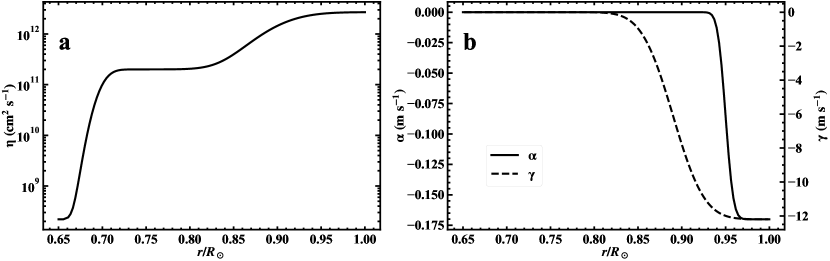
Figure 3: Radial variations of (a) turbulent diffusivity and (b) BL-type source term at -45^∘ latitude in solid line and radial pumping in dashed line, of the reference model.

We utilize the following diffusivity profile

$$\eta=\eta_{RZ}+\frac{\eta_{CZ}}{2}\left[1+\rm erf\left(\frac{r-0.7R_{\odot}}{0.03R_{\odot}}\right)\right]+\frac{\eta_{S}}{2}\left[1+\rm erf\left(\frac{r-0.9R_{\odot}}{0.05R_{\odot}}\right)\right],$$ (14)

where $\eta_{RZ}=2.2\times 10^{8}$ cm² s^-1, $\eta_{CZ}=2.0\times 10^{11}$ cm² s^-1, and $\eta_{S}=2.5\times 10^{12}$ cm² s^-1. The diffusivity at the surface is represented by $\eta_{S}$, which is close to observations and estimations based on the MLT. In the bulk of the convection zone, the diffusivity is represented by $\eta_{CZ}$, which is slightly lower than that at the surface. The diffusivity profile is shown in Figure 3(a).

3 Results

3.1 A reference model

In this section we present a representative solar-like solution, calculated with parameter values $r_{p}=0.89R_{\odot}$, $\gamma_{0}=12.2$ m s^-1, $n=6$. The profiles of the pumping and the source term at 45^∘ in the southern hemisphere are shown in Figure 3(b). For the reference case, the critical value for dipolar parity is $\alpha_{c}$ = 0.8 m s^-1. Because the solar dynamo is estimated to be about 10$\%$ supercritical (Kitchatinov & Nepomnyashchikh, 2017a), we set $\alpha_{0}$ = 0.9 m s^-1 in simulation. The solution is independent of the choice of initial conditions. After the simulation starts, transients associated with initial conditions disappear and the magnetic field grows to saturation. Here, we employ an initial field of a mixed parity. The poloidal field is set to be zero, whereas the toroidal field $B(r,\theta)$ is set to be $B(r,\theta)=\sin(2\theta)\sin[\pi(r-0.7R_{\odot})/0.3R_{\odot}]+\sin(\theta)\sin[\pi(r-0.7R_{\odot})/0.3R_{\odot}]$ for $r\geq 0.7R_{\odot}$.

Figure 4(a) shows a time-latitude diagram of the subsurface toroidal flux density calculated by integrating the toroidal field over the range of 0.7-1.0$R_{\odot}$. The toroidal field is antisymmetric since the dipolar parity always prevails in our model. The latitudinal migration pattern of the toroidal field is different from that of FTD models, which usually show concentrated flux at high latitudes due to the radial shear in the polar portion of the tachocline. For each cycle, a weak toroidal field starts from high latitudes along with another overlapped branch of the previous cycle near the equator. With the equatorward migration of the toroidal field, its flux density increases as the cycle evolutes. This scenario is consistent with that of the solar cycle and the extended solar cycle (Howard & Labonte, 1980; Wilson et al., 1988; McIntosh et al., 2014). Below 40^∘ latitude, the toroidal flux density is larger than 2.5 $\times 10^{23}$ Mx Radian^-1. Considering the spatial scale of a typical active region to be a few degrees, these fluxes are comparable with that in active regions. According to Cameron & Jiang (2019), the toroidal field at lower latitudes corresponds to the expected amount of flux residing in active regions. The weaker toroidal field at higher latitudes corresponds to ephemeral regions, which are small bipolar magnetic regions that contain a maximum total flux of the order of $10^{20}$ Mx (Harvey & Martin, 1973). In Figure 4, the vertical dashed line represents cycle minimum ($t_{min}$) when the toroidal flux of the last cycle disappears, and vertical dotted line represents cycle maximum ($t_{max}$) when the toroidal flux of the new cycle reaches a maximum. The interval between $t_{min}$ and $t_{max}$ is 4 yr, which is close to the average period of the rising phase for solar cycles (Hathaway, 2015; Jiang et al., 2018). The solid and dashed curves of Figure 5 show the time evolution of unsigned toroidal flux, $\int_{50}^{90^{\circ}}\int_{0.7R_{\odot}}^{R_{\odot}}r|B_{\phi}|\,dr\,d\theta$, of each hemisphere for odd and even cycles, respectively. The cycle period is 10.96 yr based on the interval between successive maxima of the toroidal flux. This period is consistent with the average period of observed solar activity (Hathaway, 2015). If the cycle period is calculated as the interval between the start and end of the toroidal flux of a cycle, then it is 18.1 yr. This result is consistent with approximately the 18 - 22 yr period of the extended cycle (Wilson et al., 1988). The maximum toroidal flux produced in one hemisphere is about $2.6\times 10^{23}$ Mx, which matches the observed magnetic flux at the solar surface (Cameron & Schüssler, 2015).

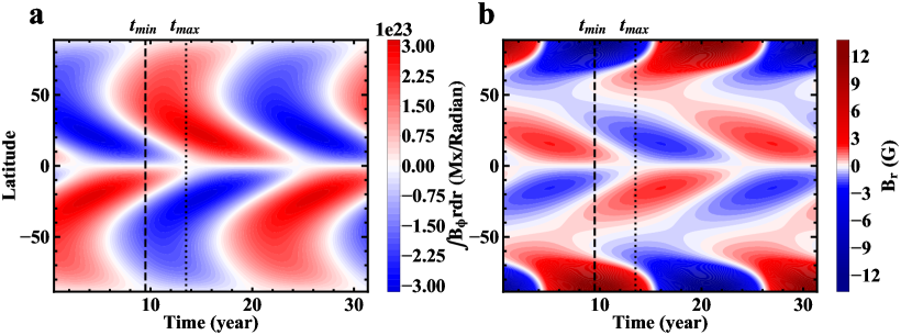
Figure 4: Time-latitude diagrams of (a) radially integrated toroidal magnetic flux (per radian) and (b) radial field at the surface, for our reference model. Cycle minimum ($t_{min}$) and cycle maximum ($t_{max}$) are indicated by the vertical dashed and dotted lines, respectively.

Figure 5: Time evolution of the subsurface toroidal flux and polar field, for the reference model. The solid and dashed curves represent the unsigned subsurface toroidal flux between $0^{\circ}$ and $40^{\circ}$ latitudes for odd and even cycles, respectively. The dotted line represents the polar field. Cycle minimum ($t_{min}$) and cycle maximum ($t_{max}$) are indicated by the vertical dashed and dotted lines, respectively.

The time-latitude diagram of $B_{r}$ at the surface is presented in Figure 4(b). There is a poleward branch and an equatorward branch that are separated by around $55^{\circ}$. The poleward branch is caused by the poleward flow and turbulent diffusion at the surface. The flux contained in this branch reverses the polar field polarity of a previous cycle and sets up the polar field of a new cycle. The equatorward branch is mainly caused by the equatorward propagation of the subsurface toroidal field that is the source of the poloidal field at the surface based on Equation (6). The maximum polar field is about 13.5 G, which is close to observational constraints (Svalgaard et al., 1978). In our model, the toroidal field in the bulk of the convection zone amounts to hundreds of gauss. The ratio of the maximum toroidal field, $B_{\phi\max}$, and maximum polar field, $B_{r\max}$, is $B_{\phi\max}/B_{r\max}$ = 45. The inward pumping compresses the poloidal field, which helps to increase the ratio between the toroidal and poloidal fields. The dotted line in Figure 5 represents the mean radial field at the surface over $70^{\circ}$ latitudes. The mean radial field reaches its maximum values about 10 G at cycle minimum corresponding to the moment when the toroidal field from the last cycle disappears. This means that our model reproduces a correct phase difference between the polar field and flux emergence at the activity belt. The polarity reversal cycle of the polar fields is also about 11 yr.

To understand how the model works, we plot the time evolution of the magnetic fields and the shear source terms for four successive intervals during a dynamo period in Figure 6. The four snapshots correspond to cycle minimum ($t_{1}$ = $t_{min}$, the first column), the time that the poloidal fields of a new cycle appear ($t_{2}$, $t_{2}$ = $t_{1}$ + 1.9 yr, the second column), cycle maximum ($t_{3}$, $t_{3}$ = $t_{2}$ + 2.1 yr = $t_{max}$, the third column), and the time that the latitudinal shear reaches a maximum ($t_{4}$, $t_{4}$ = $t_{3}$ + 4.0 yr, the fourth column).

Figures 6(a)-(d) show the poloidal field evolution. About two years after $t_{min}$, the poloidal fluxes of the new cycle appear (Figure 6(b)). The subsequent transport and evolution of the newly generated flux system have three branches. The first branch is the radially downward transport, which is determined by the radial pumping, radial component of the meridional flow, and turbulent diffusion. Above the depth of 0.88$R_{\odot}$, the pumping dominates the transport process. The pumping pushes the whole $\theta$-component of the newly generated poloidal field below the depth of 0.89$R_{\odot}$ (see Figure 6(c)). The strong pumping along with the radial boundary condition causes the poloidal field to be purely radial near the surface. This scenario is consistent with that of Cameron et al. (2012), who use SFT models to constrain the BL-type dynamo at the surface.

Figure 6: Snapshots of the poloidal field (first row), toroidal field (second row), and shear source terms (third and fourth rows) over a dynamo cycle for the reference model. Four columns from left-hand to right-hand correspond to $t_{1}$ = $t_{min}$, $t_{2}$ = $t_{1}$ + 1.9 yr, $t_{3}$ = $t_{2}$ + 2.1 yr = $t_{max}$, and $t_{4}$ = $t_{3}$ + 4.0 yr, respectively. Solid (dashed) poloidal field lines are clockwise (counterclockwise).

In the depth range 0.7-0.89$R_{\odot}$, diffusion and $u_{r}$ are responsible for the radial transport of the poloidal field. We have the simple dipolar configuration of the poloidal field threading the two poles, which is consistent with the scenario suggested by Babcock (1961). The latitudinal shear acting on $B_{\theta}$ immediately induces strong toroidal fields in the whole convection zone (see Figures 6(j), (k), and (l)). Figure 2(a) shows that in the range 0.7-0.86$R_{\odot}$ the meridional flow is equatorward. The equatorward flow is the reason for the equatorward migration of the toroidal field that is presented in Figure 4(a).

The second branch of the surface poloidal field evolution is the poleward transport. This branch is advected by the poleward meridional flow and diffusion at the surface. The poloidal field contained in this branch cancels the existing polar field from the last cycle and then reverses the polarity of the polar field (see Figures 6(c) and (d)). This explains the poleward migration of the surface field shown in Figure 4(b) corresponding to the ‘magnetic butterfly diagram’ (Hathaway, 2015). The newly generated poloidal field is simultaneously transported downward and poleward. When $B_{r}$ reaches the polar regions, $B_{\theta}$ has been transported downward to the bottom of the convection zone (see Figures 6(b) and (c)). At $t_{3}$, the source of the toroidal field $s(\textbf{B}_{\theta}\cdot\nabla_{\theta}\Omega)$ for an ‘old’ cycle has vanished and the toroidal field generation for a ‘new’ cycle starts (see Figure 6(k)). Therefore, when the polar field reverses, the subsurface toroidal field reaches a maximum at low latitudes (see Figure 6(g)).

As the cycle evolves, the newly generated poloidal flux system moves closer to the equator (panels ($b$)-($d$) of Figure 6), which corresponds to the third branch of the surface poloidal field evolution. The equatorward migration pattern is due to the equatorward migration of the subsurface toroidal field, which is the source term of the poloidal field (panels ($b$)-($d$) and ($f$)-($h$) of Figure 6). There are two causes of this equatorward migration of the toroidal field: the classical cause is the equatorward meridional flow and the second cause is a new mechanism (as follows). Figure 1(c) shows that the latitudinal shear is the strongest around 60^∘ latitudes. Its amplitude decreases at higher and lower latitudes. Hence, the toroidal field of a new cycle firstly appears around 60^∘ latitudes. It takes longer for the toroidal flux of a new cycle at lower latitudes to be built up with the weaker latitudinal shear. This regeneration pattern of the toroidal field works like the equatorward propagation. In addition, the across-equator coupling of the poloidal field leads to the final solar-like dipolar solution.

Figures 6(m)-(p) show the contribution of the radial shear to the toroidal field generation. The near-surface toroidal field generated by the radial shear in the NSSL has high-latitude poleward and low-latitude equatorward branches. The equatorward branch is dominated by the Parker-Yoshimura rule for the direction of dynamo waves (Parker, 1955; Yoshimura, 1975). The poleward branch results from the poleward migration of the surface $B_{r}$, which overpowers the dynamo wave at high latitudes. The toroidal field generated by the tachocline radial shear concentrates in the polar regions. This distribution provides strong and clear evidence that the tachocline is not the working place for our BL-type dynamo model. We further demonstrate the role of the tachocline in the following subsection.

3.2 A negligible role of the tachocline

We have shown that in our dynamo model, the toroidal field is mainly produced in the bulk of the convection zone by the latitudinal shear. The radial shear of the tachocline has a minor contribution to the toroidal field. Here, we further demonstrate the negligible role played by the tachocline in the toroidal field generation by a quantitative analysis and two numerical tests.

3.2.1 A quantitative analysis of the tachocline’s effect

Now we compare the strength of the shear source terms $s(\textbf{B}_{r}\cdot\nabla_{r}\Omega)$ and $s(\textbf{B}_{\theta}\cdot\nabla_{\theta}\Omega)$ in our reference model. Figure 7 shows results at three times, $t_{1}$, $t_{3}$, and $t_{4}$, corresponding to the first, third, and fourth columns of Figure 6, respectively. We consider the latitudinal dependence of $s(\textbf{B}_{r}\cdot\nabla_{r}\Omega)$ and $s(\textbf{B}_{\theta}\cdot\nabla_{\theta}\Omega)$ at $r=0.8R_{\odot}$ and $r=0.7R_{\odot}$, which represent the bulk of the convection zone and the tachocline, respectively.

Figure 7: Amplitude of the shear source terms as a function of latitude, at three times, $t_{1}$, $t_{3}$, and $t_{4}$, corresponding to panels (a)-(c) for the reference model. The solid curves represent the amplitude of $s(\textbf{B}_{\theta}\cdot\nabla_{\theta}\Omega)$ at middle of the convection zone, $r$ = 0.8$R_{\odot}$. The dashed and dotted curves represent the amplitude of $s(\textbf{B}_{\theta}\cdot\nabla_{\theta}\Omega)$ and $s(\textbf{B}_{r}\cdot\nabla_{r}\Omega)$ at $r$ = 0.7$R_{\odot}$, respectively.

At $t_{1}$, $s(\textbf{B}_{\theta}\cdot\nabla_{\theta}\Omega)$ at $r=0.8R_{\odot}$ (Figure 7(a), solid curve) peaks around 25^∘ and 70^∘. The average strength over latitudes $\langle s(\textbf{B}_{\theta}\cdot\nabla_{\theta}\Omega)\rangle$ is 8.8 G s^-1, which is about three times the value at $r=0.7R_{\odot}$ (dashed curve). The term $s(\textbf{B}_{r}\cdot\nabla_{r}\Omega)$ at $r=0.7R_{\odot}$ (dotted curve) peaks around 80^∘. Its latitudinal averaged strength, $\langle s(\textbf{B}_{r}\cdot\nabla_{r}\Omega)\rangle$, is 1.9 $\times 10^{-3}$ G s^-1, which is about one fifth of $\langle s(\textbf{B}_{\theta}\cdot\nabla_{\theta}\Omega)\rangle$ at $r=0.8R_{\odot}$. If we exclude the values above 50^∘, $\langle s(\textbf{B}_{r}\cdot\nabla_{r}\Omega)\rangle$ is close to zero. At $t_{1}$, the shear strength is decaying because the poloidal field is being canceled. About two years from $t_{1}$, the poloidal fluxes of the new cycle appear at the surface (Figure 6(b)). It takes about two years to transport these fluxes to the poles and the bottom of the convection zone. Therefore, at $t_{3}$ (Figure 7(b)) the sign of $s(\textbf{B}_{\theta}\cdot\nabla_{\theta}\Omega)$ changes and the toroidal field of the new cycle, whose polarity is opposite to that of the previous cycle, begins producing at middle latitudes (see Figure 6(g)). The distribution of $s(\textbf{B}_{\theta}\cdot\nabla_{\theta}\Omega)$ at $r=0.8R_{\odot}$ peaks around 50^∘. With the continuous generation and downward diffusion of the newly generated poloidal fields, the strength of $s(\textbf{B}_{\theta}\cdot\nabla_{\theta}\Omega)$ reaches a maximum at $t_{4}$ (Figure 7(c)). At this moment, the average strength of $s(\textbf{B}_{\theta}\cdot\nabla_{\theta}\Omega)$ at $r=0.8R_{\odot}$ is 9$\times 10^{-3}$ G s^-1, which is about 30 times the value at $r=0.7R_{\odot}$. The average strength of the radial shear is 0.4 $\times 10^{-3}$ G s^-1 at $r=0.7R_{\odot}$, which is one twentieth of the average value of $s(\textbf{B}_{\theta}\cdot\nabla_{\theta}\Omega)$ at $r=0.8R_{\odot}$. If we exclude the values above 50^∘, $\langle s(\textbf{B}_{r}\cdot\nabla_{r}\Omega)\rangle$ at $r=0.7R_{\odot}$ is also close to zero.

Based on the quantified analysis of the shear strength at the three moments, we confirm that most toroidal fluxes come from the latitudinal shear in the bulk of the convection zone. The radial and latitudinal shear in the tachocline have a weak contribution to the toroidal field.

3.2.2 Numerical experiments

In the reference model, the differential rotation profile is based on helioseismic results, including the tachocline characterized by the strong radial shear at the base of the convection zone. Since the tachocline has been shown to play a minor role in our dynamo model, we now carry out numerical experiments to check the dynamo behavior by artificially shutting off the tachocline in two ways.

Figure 8: Same as Figure 4, but panels (a) and (b) for the case with the differential rotation shown in Figure 1(b); panels (c) and (d) for the case with the bottom boundary at 0.725$R_{\odot}$.

In the first experiment, we use the differential rotation profile shown in Figure 1(b) to artificially remove the radial shear in the tachocline. The latitudinal shear of the tachocline is still included in the experiment, but it is slightly stronger than that of the original profile. We keep the other ingredients of the model the same as those in the reference model, including other model parameters, initial and boundary conditions, except $\alpha_{0}$ and $\eta_{CZ}$. Since the average strength of the latitudinal shear in the first experiment is stronger than that in the reference model, as shown in Figures 1(c) and (d), to keep $\nabla\Omega R_{\odot}^{2}/\eta$ in this experiment, consistent with that in the reference model, we use a larger diffusivity, $\eta_{CZ}=2.9\times 10^{11}$ cm² s^-1, than that in the reference model. Accordingly, a 10$\%$ supercritical $\alpha_{0}$ = 0.92 m s^-1 is used. The results are shown in Figures 8 (a) and (b), which are derived in the same way as those in Figure 4. The solution has a 11.4 yr cycle period and a similar field distribution as that of the reference model.

In the second experiment, we set the bottom boundary at a depth of 0.725$R_{\odot}$, which means that the effects of the tachocline on the dynamo model are completely removed. The penetration depth of the meridional flow is changed to $r_{b}$ = 0.725$R_{\odot}$. The parameter $\psi_{0}/C$ is changed to 39.1 m s^-1 to ensure a maximum surface flow of 20 m s^-1. We use $\eta_{CZ}=3.1\times 10^{11}$ cm² s^-1 and $\alpha_{0}$ = 0.63 m s^-1 in this case, for the same reason shown in the first experiment. The other parameters are the same as those in the reference model. The results are shown in Figures 8 (c) and (d). The dynamo could also operate successfully for this case. Both the toroidal and poloidal fields show a similar pattern as those in the reference model, and the cycle period is 11.1 yr. In summary, the two numerical tests further confirm the negligible role played by the tachocline in our model.

3.3 Comparison with Other representative models

Dikpati & Charbonneau (1999), hereafter DC1999, and Chatterjee et al. (2004), hereafter CNC2004, are two representative FTD models. Yeates et al. (2008) gave a close investigation of the two models. Here, we compare our reference model, hereafter ZJ2021, with them to illustrate the differences among the models. To reproduce DC1999, we take the set of parameters listed in their Section 3. The only difference is that we extend the solution to both the northern and southern hemispheres rather than only the northern hemisphere, as used in their model. For CNC2004, we use the parameters in their Section 3.1. Figure 9 shows the time evolution of the poloidal and toroidal fields in the two models for four successive intervals during a half of the dynamo period.

Figure 9: Snapshots of the poloidal field (first and second rows) and toroidal field (third and fourth rows) for model CNC2004 (first and third rows) and model DC1999 (second and fourth rows) over one half cycle for comparison with the reference model shown in Figure 6. Each column is advanced by an eighth of the dynamo cycle; that is, from left-hand to right-hand $t$ = 0, $T$/8, $T$/4, and 3$T$/8. Solid (dashed) poloidal field lines are clockwise (counterclockwise).

A prominent difference among the three models is the configuration of the poloidal field. In our model, the poloidal field is highly organized. The near-surface field is purely radial. At cycle minimum, the poloidal field has a global and simple dipolar structure. Panels ($a$)-($d$) of Figure 9 show the poloidal field evolution from CNC2004. Although there is also a cross-equator connection of the poloidal field that is similar to ours, dissipation of the poloidal field crossing the surface exists. Circular structures of the poloidal field near the surface are an implication of the dissipation and correspond to a strong $B_{\theta}$ component, which is not consistent with the prerequisite of the empirical SFT models (Cameron et al., 2012). Panels ($e$)-($h$) of Figure 9 show the poloidal field evolution from DC1999. The poloidal field has a complex configuration. In contrast to the global structure in our model, several local structures in both latitudinal and radial directions are presented here. Moreover, the poloidal fields in two hemispheres have an antisymmetric structure, which corresponds to a quadrupolar solution.

Besides the different outer boundary conditions (vertical versus potential), the different flux transport mechanisms of the poloidal field are mainly responsible for the different configurations of the poloidal field. In our model, the downward pumping along with the radial outer boundary condition keeps the poloidal field radial near the surface. The strong turbulent diffusion dominates the poloidal field transport through the bulk of the convection zone. Since the polar field is radial, the meridional flow, which is also radial near the poles, cannot subduct the polar field into the interior. However, in both CNC2004 and DC1999, there is a subduction of the poloidal field by the meridional flow sinking underneath the surface at the polar regions. The subducted flux plays a significant role in their magnetic field evolution (Hazra et al., 2017). Especially in DC1999, the meridional flow dominates the transport of the poloidal field. The surface polar field dominated by the $B_{\theta}$ component is advected downward to the tachocline. Figure 9(h) shows the highly concentrated polar field, which causes a low ratio of $B_{\phi\max}/B_{r\max}$. The strong polar field and weak ratio of $B_{\phi\max}/B_{r\max}$ have been regarded as difficulties of the model. In CNC2004, a part of the newly generated poloidal fields is transported downward by diffusion. Compared with our model, the downward $B_{\theta}$ is relatively weak because a part of the poloidal fields is dissipated across the surface. All of these ingredients cause the poloidal field evolution, including the polar field evolution, among the three models to be strikingly different.

Different configurations of the poloidal field further determine where the toroidal field is produced. In our model, the poloidal field has a global scale and is $\theta$-component dominated in the bulk of the convection zone. This poloidal field configuration determines that most toroidal fields are produced by the latitudinal shear in the bulk of the convection zone. The latitudinal shear peaks around middle latitudes. Along with the effect of the equatorward meridional flow, most of the toroidal fields are produced at mid-low latitudes. There are no strong toroidal fields at the polar regions. In CNC2004, there is a quite strong $B_{\theta}$ distribution in the bulk of the convection zone, but $B_{\theta}$ in the tachocline is even stronger. There is a certain amount of $B_{r}$ in the tachocline. Hence, the newly generated toroidal field concentrates at the bottom of the convection zone (see Figures 9(i)-(l)). Both the latitudinal and radial shears of the tachocline contribute to the toroidal field generation. Muñoz-Jaramillo et al. (2009) have pointed out that the latitudinal shear is dominated in producing the toroidal field in models with a high diffusivity. In DC1999, effects of the latitudinal shear on the toroidal field generation were also addressed. Since the poloidal field is dominated by the $r$-component in the tachocline, the radial shear of the tachocline contributes most to the toroidal field generation (see Figures 9(m)-(p)). The radial shear of the tachocline peaks at high latitudes. The concentrated toroidal field at high latitudes is inevitable. Note that in both CNC2004 and DC1999, the toroidal field concentrates below 0.75$R_{\odot}$ (see panels (i)-(p) of Figure 9), which is strikingly different from our reference model.

Figure 10: Comparison of the time evolution of the magnetic energy ratio, $\frac{E_{\theta}}{E_{all}}$ defined by Eq.(15) among ZJ2021 (solid line), CNC2004 (dashed line), and DC1999 (dotted line).

We now give a quantitative comparison of the relative strength of $B_{\theta}$ among the three models. Figure 10 shows the time evolution of the magnetic energy ratio of

$$\frac{E_{\theta}}{E_{all}}=\frac{\int_{0.7R_{\odot}}^{0.89R_{\odot}}\int_{30^{\circ}}^{90^{\circ}}B_{\theta}^{2}r^{2}\sin\theta\,dr\,d\theta}{\int_{0.7R_{\odot}}^{R_{\odot}}\int_{0^{\circ}}^{90^{\circ}}(B_{\theta}^{2}+B_{r}^{2})r^{2}\sin\theta\,dr\,d\theta}.$$ (15)

The maximum value of $E_{\theta}/E_{all}$ in our reference model is 0.8, which is about twice as large as that of CNC2004 and about 20 times larger than that of DC1999. During the whole period, $B_{\theta}$ dominates the poloidal field in our model.

In summary, our model has a prominently different configuration of the poloidal field from that of DC1999 and CNC2004. Different flux transport mechanisms and outer boundary conditions account for the different poloidal field configurations, which lead to the different locations of the toroidal field generation.

4 Conclusion

We have developed a new BL-type solar dynamo model, in which the toroidal field is generated in the bulk of the convection zone by the latitudinal differential rotation. The radial shear in the tachocline plays a negligible role in the toroidal field generation. This distinguishes our model from the popular view that the tachocline is the location of the toroidal magnetic flux production, yet fulfills the needs of recent advances in the understanding of solar magnetism (as listed in our introduction). The model satisfactorily reproduces the following major solar cycle features: (1) about 11 yr cycle period and 18 yr extended cycle period, (2) the equatorward migration of the toroidal fields and the poleward drift of the large-scale surface radial fields, (3) the realistic phase relation between the polar field and the toroidal field, and (4) a solar-like antisymmetric magnetic field about the equator. We have also carried out two numerical experiments to check the dynamo behavior by artificially shutting off the tachocline. These two experiments show similar solutions to the reference model.

Our model has several advantages as compared with DC1999 and CNC2004 due to the following facts. First, the strong polar branch of the toroidal field is circumvented in our model. The toroidal flux of each cycle starts from the polar region, with weak strength corresponding to ephemeral regions. With the equatorward migration of the toroidal flux, its strength increases and corresponds to active regions at middle and low latitudes. Thus, the results account for not only the solar cycle but also the extended cycle. In contrast, the strong polar branch is a typical property of the FTD models working in the tachocline. To remove the branch, additional assumptions have to be included, such as the deep penetration of the meridional flow (Nandy & Choudhuri, 2002; Chatterjee et al., 2004).

Second, we obtain a solar-like antisymmetric magnetic field about the equator with the pure BL-type $\alpha$-effect alone in our model. An extra $\alpha$-effect is required in FTD models to account for the dipolar solution (e.g., Dikpati et al., 2004; Passos et al., 2014). Third, the toroidal and poloidal fields have the same strong diffusivity, which is 2$\times 10^{11}~{}$cm²s^-1 in the bulk of the convection zone. It is still weaker than the estimated value based on the MLT but is one order higher than the value used in previous FTD models. The quenching of the turbulent diffusivity for the toroidal field, which is adopted by CNC2004, is not plausible based on Karak et al. (2014).

The most significant advantage of our model lies in producing a realistic configuration and evolution of the polar field. The polar field peaks around the cycle minimum, with an amplitude of about 10 G. It is radial, hence there is no subduction of the polar flux by the radially downward meridional flow sinking underneath the surface. Thus, the evolution of the polar field is purely due to the flux transport from the activity belt. In contrast, previous FTD models tend to generate a polar field that is too strong (e.g., Durney, 1997; Dikpati & Charbonneau, 1999; Hazra et al., 2017). The meridional flow subducts the polar field sinking underneath the surface. The polar flux submergence plays an important role in their polar field evolution.

One of the reasons for the effectiveness of our model is that it includes near-surface radial pumping and a radial outer boundary condition. These ingredients are derived from the constraints of surface flux evolution by Cameron et al. (2012) and they lead to a simple dipolar configuration of the poloidal field, which contains the purely radial field near the surface and the latitudinal field within the convection zone. Consequently, the latitudinal shear winds up the global dipole to produce most of the toroidal fields in the bulk of the convection zone. This model is consistent with Babcock’s original scenario. The BL-type solar dynamo models developed by Kitchatinov & Olemskoy (2012) and Kitchatinov & Nepomnyashchikh (2017b) also do not depend on the tachocline. In addition, the diamagnetic pumping is included in their models, but the downward pumping is very efficient near the bottom of the convection zone. As a result, although the toroidal field is not generated in the tachocline, it is near the base of the convection zone ($\sim 0.72-0.81R_{\odot}$), where the diffusivity has a rapid variation over 3 orders, from lower than $10^{9}$ cm² s^-1 to higher than $10^{12}$ cm² s^-1. Furthermore, because the radial field assumption is not satisfied, the evolution of the surface field cannot be guaranteed to be consistent with that of the SFT models.

The flux transport mechanisms are another reason for our model’s success. The generating layers of toroidal and poloidal fields are spatially segregated in FTD models. Toroidal and poloidal fields are connected by flux transport mechanisms, especially the meridional flow. The meridional flow plays an essential role in regulating the cycle period and the equatorward migration of the toroidal field in FTD models. In contrast, the generation layers of toroidal and poloidal fields are partially coupled in our model, due to the effect of surface radial pumping. Furthermore, the meridional flow cannot transport the polar flux sinking under the surface. Hence, our model is less reliant on the inner structure of the meridional flow than FTD models. In a forthcoming paper, we will explore this property in detail.

References

- Babcock (1961) Babcock, H. W. 1961, ApJ, 133, 572, doi: 10.1086/147060
- Basu & Antia (2010) Basu, S., & Antia, H. M. 2010, ApJ, 717, 488, doi: 10.1088/0004-637X/717/1/488
- Baumann et al. (2004) Baumann, I., Schmitt, D., Schüssler, M., & Solanki, S. K. 2004, A&A, 426, 1075, doi: 10.1051/0004-6361:20048024
- Brandenburg (2005) Brandenburg, A. 2005, ApJ, 625, 539, doi: 10.1086/429584
- Brandenburg et al. (1992) Brandenburg, A., Moss, D., & Tuominen, I. 1992, in Astronomical Society of the Pacific Conference Series, Vol. 27, The Solar Cycle, ed. K. L. Harvey, 536
- Caligari et al. (1995) Caligari, P., Moreno-Insertis, F., & Schussler, M. 1995, ApJ, 441, 886, doi: 10.1086/175410
- Cameron & Schüssler (2015) Cameron, R., & Schüssler, M. 2015, Science, 347, 1333, doi: 10.1126/science.1261470
- Cameron & Jiang (2019) Cameron, R. H., & Jiang, J. 2019, A&A, 631, A27, doi: 10.1051/0004-6361/201834852
- Cameron et al. (2012) Cameron, R. H., Schmitt, D., Jiang, J., & Işık, E. 2012, A&A, 542, A127, doi: 10.1051/0004-6361/201218906
- Cameron & Schüssler (2017a) Cameron, R. H., & Schüssler, M. 2017a, A&A, 599, A52, doi: 10.1051/0004-6361/201629746
- Cameron & Schüssler (2017b) —. 2017b, ApJ, 843, 111, doi: 10.3847/1538-4357/aa767a
- Charbonneau (2016) Charbonneau, P. 2016, Nature, 535, 500, doi: 10.1038/535500a
- Charbonneau (2020) —. 2020, Living Reviews in Solar Physics, 17, 4, doi: 10.1007/s41116-020-00025-6
- Chatterjee et al. (2004) Chatterjee, P., Nandy, D., & Choudhuri, A. R. 2004, A&A, 427, 1019, doi: 10.1051/0004-6361:20041199
- Chen et al. (2021) Chen, F., Rempel, M., & Fan, Y. 2021, arXiv e-prints, arXiv:2106.14055. https://arxiv.org/abs/2106.14055
- Choudhuri (2021) Choudhuri, A. R. 2021, Science China Physics, Mechanics, and Astronomy, 64, 239601, doi: 10.1007/s11433-020-1628-1
- Choudhuri et al. (1995) Choudhuri, A. R., Schussler, M., & Dikpati, M. 1995, A&A, 303, L29
- Dasi-Espuig et al. (2010) Dasi-Espuig, M., Solanki, S. K., Krivova, N. A., Cameron, R., & Peñuela, T. 2010, A&A, 518, A7, doi: 10.1051/0004-6361/201014301