Part
Accelerating nuclear-norm regularized low-rank matrix optimization through Burer-Monteiro decomposition
Abstract
This work proposes a rapid algorithm, BM-Global, for nuclear-norm-regularized convex and low-rank matrix optimization problems. BM-Global efficiently decreases the objective value via low-cost steps leveraging the nonconvex but smooth Burer-Monteiro (BM) decomposition, while effectively escapes saddle points and spurious local minima ubiquitous in the BM form to obtain guarantees of fast convergence rates to the global optima of the original nuclear-norm-regularized problem through aperiodic inexact proximal gradient steps on it. The proposed approach adaptively adjusts the rank for the BM decomposition and can provably identify an optimal rank for the BM decomposition problem automatically in the course of optimization through tools of manifold identification. BM-Global hence also spends significantly less time on parameter tuning than existing matrix-factorization methods, which require an exhaustive search for finding this optimal rank. Extensive experiments on real-world large-scale problems of recommendation systems, regularized kernel estimation, and molecular conformation confirm that BM-Global can indeed effectively escapes spurious local minima at which existing BM approaches are stuck, and is a magnitude faster than state-of-the-art algorithms for low-rank matrix optimization problems involving a nuclear-norm regularizer.
1 Introduction
Consider the following regularized convex matrix optimization problem
| (CVX) |
where the loss term is lower-bounded, convex, and differentiable with Lipschitz-continuous gradient, and the regularizer is convex and has the form
| (1) |
with being a closed and convex subset of . Clearly, in this case, is nonsmooth, convex, proper, and closed.111Note that when and is a subset of , is convex, proper, and closed even if , as in that case the nuclear norm becomes the trace of , which is an affine function of . Otherwise, we will need to make convex. Without loss of generality, we assume that throughout, which can be achieved easily by conducting a matrix transpose if necessary. For our case of Eq. 1, as long as is properly selected, a low-rank optimal solution to Eq. CVX exists, since the nuclear norm is exactly applying the -norm to the singular values of the given matrix. In practice, singular value decomposition (SVD) for a non-symmetric matrix is calculated through the eigendecomposition of the symmetric matrix (as we assume ), and thus computation of SVDs and of eigendecompositions are nearly identical. We will therefore summarize these two situations simply as requiring eigendecompositions.
We focus on large-scale problems such that is extremely large, so forming a (possibly dense) matrix explicitly is spatially and computationally expensive, if not infeasible, and thus a low-rank solution is necessary for practical reasons. The nuclear-norm regularization hence serves to induce a low-rank structure in any solution to Eq. CVX. On the other hand, we assume that is either structured or extremely sparse so that for any vector can be computed efficiently. This is necessary for the execution of an inexact proximal gradient (PG) step; see details in Section 3.
To deal with the high problem dimensionality in Eq. CVX, a popular approach is the Burer-Monteiro (BM) decomposition (BurM03a) that explicitly writes as a product of two low-rank matrices with a pre-specified rank . Explicitly, we get
| (BM) |
The spatial cost of for storing in Eq. CVX is then reduced to in Eq. BM. Numerous efficient algorithms for solving Eq. BM are therefore proposed.
Among applications of Eq. CVX, one of the most prominent example, and also our motivating problem, is the following low-rank matrix completion problem whose target is to recover the whole ground truth matrix from its observed entries enumerated by an index set :
| (MC) |
where is the Frobenius norm and
It is well-known that the factorized form in Eq. BM of Eq. MC for a given rank is
| (MF) |
which is often called the matrix factorization (MF) problem in the machine learning community. One can easily show that the global optimal objectives of Eq. MC and Eq. MF coincide whenever is large enough such that there is at least one optimal solution of Eq. MC with . (See Lemma 1.) Apparently, even the objective evaluation for Eq. MC requires an eigendecomposition that costs , while for Eq. MF, objective evaluation and variable updates all require cost of only .
Unfortunately, the lower computational and spatial costs of solving Eq. MF and thus the more general Eq. BM comes with a price. A disadvantage of the BM method is that the rank needs to be specified in advance, and a good value for can be hard to estimate a priori. Another even more severe issue is that the problem Eq. MF is a nonconvex one, meaning that algorithms for solving it could get stuck at spurious local optima (local but not global optima) or saddle points that have a zero gradient. Such points can give terrible performance for predicting missing entries. The simplest example would be that for any , letting and be matrices of all zeros in Eq. MF will directly generate a saddle point, but this clearly is not a solution in general. It is also recently shown by (YalZLS22a; OcaSV22a) that there are indeed problems with a sufficiently large that still possess spurious local minima with a terribly large objective value, and thus how to escape from such saddle points and spurious local minima is critical issue for the BM approach to produce satisfactory performance.
On the other hand, the convex problem Eq. MC or Eq. CVX can be solved directly through PG-type algorithms that are able to find the global optima (TohY10a), but the cost of the eigendecomposition in the proximal operation is extremely expensive, even if only a subset of singular values/vectors is required. State-of-the-art methods for Eq. MC like those by (HsiO14a; YaoKWL18a) thus resort to approximate eigendecompositions computed through the power method to reduce the time cost of eigendecompositions. The power method also has the benefit that only for some thin matrix is needed at each iteration, so explicit computation of is not needed. However, we observe that in practice, usually the convex approaches based on PG tend to be rather slow because their computational cost per iteration is still not comparable to those for Eq. MF or Eq. BM.
In this work, we propose a highly-efficient algorithm, BM-Global, that combines the advantages of both approaches with theoretical guarantees. Our method fully utilizes the computational and spatial advantages of Eq. BM to have a running time similar to the state-of-the-art for Eq. BM. Meanwhile, BM-Global also possesses guarantees for convergence to the global optima just like those approaches for solving Eq. CVX. With suitable inexactness conditions for the PG steps, we also obtain a sublinear convergence rate for the general convex case, and further get faster rates when the objective function satisfies the Kurdyka-Łojasiewicz (KL) condition (Kur98a; Loj63a). Our algorithm attains these appealing guarantees through sporadically resorting to convex lifting steps that conduct one iteration of inexact PG on Eq. CVX to escape from saddle points and spurious local optima at which existing methods for Eq. BM got stuck at. We emphasize that for alternating between inexact PG and other update steps, our convergence and rate guarantees are novel, as existing analyses for convergence and rates of inexact PG rely on geometrical properties of the PG iterates that will be destroyed when other updates are inserted.
Through the techniques of manifold identification (HarL04a; LewZ13a) in our analysis, another major and novel contribution of this work is that the optimal rank for Eq. BM will provably be found by the proposed method automatically, so no additional parameter tuning for the optimization side is required for attaining satisfactory results for practical applications of Eq. CVX. Numerical results also show that our method is significantly faster than state-of-the-art solvers for Eq. CVX, and can effectively escape from saddle points and spurious local minima of Eq. BM.
1.1 Related Works
Methods for Eq. CVX. The convex problem Eq. CVX falls in the category of regularized optimization, and many efficient algorithms in the literature are available. However, most methods for regularized optimization concentrate on the scenario that the proximal operation can be conducted efficiently but obtaining information of the smooth term is the major computational bottleneck, which is apparently not the case for Eq. CVX. Practical methods specifically designed for Eq. CVX all take into serious account the expensive SVD involved in the nuclear norm (TohY10a; HsiO14a; YaoKWL18a), and they all focus on the most popular setting that is a quadratic term. In this case, high-order methods like proximal (quasi-)Newton is useless because the subproblem has the same form as the original problem itself. Therefore, these works all consider first-order methods such as the (inexact) PG or accelerated PG (APG) methods (Nes13a; BecT09a; BecT09b). TohY10a used the Lanczos method to conduct approximate SVD, and HsiO14a proposed to apply the power method for approximate SVD and to use the rank decided by their inexact PG method to conduct another convex optimization step with respect to a subproblem of dimension after each PG step. The power method in (HsiO14a) effectively uses the current iterate as warmstart and is much more efficient than the Lanczos approach in (TohY10a), but the additional convex optimization step turns out to be time-consuming. To improve the efficiency of (TohY10a) and (HsiO14a), YaoKWL18a combined the two approaches to turn to inexact APG using the power method.
More recently, motivated by PG’s ability of manifold identification, (BarIM20a) proposed to alternate between an exact PG step and a Riemannian (truncated) Newton step on the currently identified manifold for general regularized optimization, and applied this method to a toy problem of Eq. CVX in their experiments. Different from ours, their usage of manifold identification is for showing that their method could obtain superlinear convergence, but their algorithm is not feasible for large-scale problems considered in this work because they considered exact PG only and required the explicit computation of .
Convergence of Inexact Proximal Gradient The global convergence of our method is achieved through the safeguard of inexact PG steps, but we do not require the inexact PG step to always decrease the objective value. This feature combined with the BM phase makes the analysis difficult. Existing analyses for inexact PG (Com04a; SchRB11a; JiaST12a; HamWWM22a) utilize telescope sums of inequalities in the form of for any and some to prove convergence and rates. Therefore, those approaches cannot allow for alternating between inexact PG and other steps because that will nullify the technique of telescope sums. On the other hand, analyses compatible with other steps like those in (SchT16a; BonLPP16a; LeeW18a) require strict decreasing of the objective in the inexact PG step (either explicitly or implicitly), which imposes an additional burden.
The work of (YanLCT21a) that applies inexact PG to the semidefinite programming (SDP) relaxation of polynomial optimization problems is probably the closest to our approach in that their method alternates between nonmonotone inexact PG and an alternative step. However, their alternative step is only accepted when it decreases the objective by an absolute amount , so eventually the alternative steps are always rejected when the objective converges, but we do not have such restrictions. Our analysis also provides more comprehensive convergence guarantees under different conditions as well as identification of the optimal rank using techniques totally different from that of (YanLCT21a).
Methods for escaping saddle points. There has recently been a thriving interest in studying smooth optimization methods that can escape strict saddle points with at least one negative eigenvalue in the Hessian (LeePPSJR19a; JinGNKJ17a; RoyW18a; CarDHS18a; RoyOW20a; AgaABHM17a). However, these methods are unable to deal with degenerate saddle points where the smallest eigenvalue of the Hessian is exactly zero, and neither could they deal with spurious local minima that might be arbitrarily far away from the global ones. On the other hand, our method can handle all such difficult cases appearing in Eq. BM by resorting to convex lifting, and Lemma 1 together with Theorem 2 show that our method indeed will converge to the global optima. Moreover, existing methods for escaping strict saddles are mainly of theoretical interest, and their empirical performance is usually not very impressive, while our method is designed for practical large-scale usage and greatly outperforms state-of-the-art methods for Eq. CVX and Eq. BM by a large margin on real-world data, as we shall see in the numerical experiments later.
Absence of spurious stationary points for Eq. MF. To cope with possible spurious local minima and degenerate saddle points of matrix factorization, there is also a growing interest in analyzing its optimization landscape. Most such works consider the quadratic loss:
| (2) |
(GeLM16a; SunL16a; GeJZ17a) confined their analyses to Eq. 2 and proved the absence of spurious local minima for only the ideal case in which each belongs to with a fixed probability and the observations are noiseless. But these assumptions generally fail in practice. In particular, for applications like recommendation systems, elements of are already biased selections by an existing system and will never obey the independent random assumption. In addition, real-world data always contain noisy observations and measurement corruption. (CheCFM19a; YeD21a) focused on Eq. 2 with only, and their techniques could be hard to generalize to other problems. Moreover, these two works discussed only the gradient descent method, which is barely used (if any) in large-scale real applications. Different from these works, we do not have any assumption on the underlying data, as it has been shown recently in (YalZLS22a; OcaSV22a) that some problem classes of matrix factorization and SDP indeed contain numerous spurious local minima, yet our method can still find the global optima in the presence of non-strict saddle points and spurious local optima with ultra-high practical efficiency.
1.2 Organization
This paper is organized as follows. Preliminaries for our algorithmic development are provided in Section 2. In Section 3, we describe our main algorithmic framework. Section 4 provides a comprehensive theoretical analysis of our algorithm, including its global convergence to the global optima, convergence rates, and identification of the right rank for Eq. BM within a finite number of iterations. We then give more details in Section 5 several realizations of Eq. CVX in applications. Numerical experiments on real-world problems in such applications are conducted in Section 6, and finally Section 7 concludes this work. Detailed implementations for the applications used in our numerical experiments and additional experimental results are provided in the supplementary materials starting from Page Part.
2 Preliminaries
This section first lays out our notations in this work, and then provides background knowledge that will facilitate further descriptions in our development of algorithm and theory. We use to denote the trace of a square matrix. For any , is the diagonal matrix whose diagonal entries are those in . We use to denote the standard inner product and to denote its induced norm. In particular, for vectors , this is the standard inner product such that , with the norm being the Euclidean norm, and for matrices , this inner product is defined as , where is the transpose of and the corresponding norm is the Frobenius norm. We denote by the nonnegative orthant in the -dimensional Euclidean space, by the set of by symmetric real matrices, and by the cone of symmetric positive semidefinite matrices in . denotes the identity matrix with dimension , and is the vector of ones. The subscript is often omitted when the dimensionality is clear. For , we let be its Euclidean projection onto , and for , is its Euclidean projection onto . In particular, if admits an eigendecomposition , where is orthonormal such that and , we have that . We note that SVDs and eigendecompositions are unique up to permutations of the eigenvalues or the singular values, so we will simply say “the” SVD or “the” eigendecomposition to refer to the one such that the singular values or eigenvalues are sorted in descending order. (And this can be an arbitrary one when there are repeated singular values.) Given any set , we use to denote its indicator function such that
For any convex function , we use to denote its subdifferential.
Throughout this work, we will heavily use the proximal operation. Given a function , this operation is defined as
| (3) |
For convex, proper, and closed, it is well-known that Eq. 3 is well-defined and single-valued everywhere. When for some , Eq. 3 has a closed-form solution (LewO96a). Given a matrix with rank and with its SVD written as for some that are orthogonal and , we have
| (4) |
for any . Similarly, if admits an eigendecomposition , we have from (LewO96a) that for any ,
| (5) |
In this paper, we focus on the two scenarios of and (for ) for some closed and convex set . We will see in Lemma 1 that the former results in the following form of Eq. BM:
| (BM-nuclear) |
while the latter leads to
| (BM-PSD) |
For the latter case, when we deal with Eq. CVX, for easier calculation, we will sometimes consider the smooth term as and the regularizer as instead, which is equivalent to the original problem because the nuclear norm on a positive semidefinite matrix is exactly the trace of the same matrix.
The equivalence between the nuclear norm in Eq. CVX and the Frobenius norm squared in Eqs. BM-nuclear and BM-PSD is formally stated in the following lemma.
Lemma 1.
Given any , we have
| (6) |
Moreover, if the SVD of is
where and are the singular values, , and are both orthonormal, the minima of the right-hand side of Eq. 6 are exactly those
| (7) |
where is an arbitrary random permutation of . Therefore, for any global optimum of Eq. BM-nuclear, is also a global optimum to Eq. CVX with , provided that there is a global optimum of Eq. CVX with , and for any optimal solution of Eq. CVX with SVD ,
form a global solution of Eq. BM-nuclear for any . Likewise, for any global optimum of Eq. BM-PSD, is also a global optimum to Eq. CVX with , provided that there is a global optimum of Eq. CVX with .
3 Algorithmic framework
In this section, we present a detailed description of the proposed BM-Global that can be split into two phases: the BM phase and the convex lifting phase. The high-level idea of the proposed framework is to fully utilize the efficiency in solving Eq. BM from the smoothness of the objective function whenever possible. When only limited progress can be further made in the BM phase with the current iterate , we turn to the convex lifting phase, which conducts one step of inexact proximal gradient (PG) on Eq. CVX from the iterate . In the inexact PG step, an approximate eigendecomposition algorithm is employed to obtain the next iterate . The rank of the approximate eigendecomposition is dynamically increased (and the proximal step decreases the rank of its output) to guarantee that the correct rank at the optimum can be found within finite iterations of our algorithm.
We note that Eq. 7 provides a convenient way to transform an iterate of Eq. CVX to that of Eq. BM-nuclear or Eq. BM-PSD. (Transforming the other way round is straightforward.) Although this transformation requires an eigendecomposition, we will see shortly that our convex lifting step will generate the exact eigendecomposition of its output (which is obtained from conducting an exact proximal operation on an approximate eigendecomposition of the input matrix), so the transformation can be done almost for free. We emphasize that the matrix is never explicitly formed when executing BM-Global.
The only requirement we put on the BM phase is a mild and implementable nonincreasing objective condition:
| (8) |
Therefore, we can also skip the BM phase from time to time without violating Eq. 8 when this skipping is deemed useful.
In the convex lifting phase, we emphasize that since we never explicitly store the dense matrix variable due to the high spatial cost, exact decomposition for computing the eigendecomposition becomes impractical. This is one of the major reasons to consider approximate eigendecompositions that are computed through an iterative process where each iteration of which only requires the computation of matrix-matrix products of the form for some thin matrix . This product can be computed efficiently without explicitly forming if can be decomposed into the sum of a low-rank matrix and a highly sparse matrix. This is another reason to consider low-rank problems promoted by the nuclear norm, as the proximal operation of the nuclear norm often leads to a low-rank iterate. See more details in Eqs. 4 and 5, and Theorem 6 in Section 4.
Although state-of-the-art for Eq. CVX such as the works of (TohY10a; YaoKWL18a) utilizes the APG method (BecT09a; Nes13a) to obtain theoretical and practical convergence faster than that of the PG method, APG is not applicable in our framework because the meaning of its extrapolation step becomes unclear when we insert other update steps between two APG iterations. Moreover, although using a vanilla PG method in our algorithm results in a slower worst-case convergence rate than the APG method, our major workhorse in reducing the objective value efficiently is actually the BM phase, while our PG step mainly serves as a safeguard for global convergence and the mechanism to identify the correct rank. Therefore, we do not expect the PG step to provide much objective decrease empirically. In the numerical experiments, we will also see that the added BM phase indeed effectively decreases the objective value with a short running time, making the proposed algorithm outperform the APG method of (TohY10a; YaoKWL18a) significantly.
3.1 Inexact Proximal Gradient Step
Given the iterate and a step size at the th iteration, the exact PG step is computed by
| (9) | ||||
After finding a suitable ensuring a sufficient decrease in , the exact PG method then assigns . For our inexact scheme, we focus on the scheme that the computation of and the proximal operation in Eq. 4 or Eq. 5 are exact, and the inexactness in the PG step comes from the approximate eigendecomposition. In particular, the approximate eigendecomposition is the exact eigendecomposition of a matrix approximating the original one, and thus we can easily conduct exact eigenvalue/singular value truncation in Eq. 4 or Eq. 5 of this approximation matrix.
We can therefore view the calculation of our inexact PG step with such an inexactness quantified by some as
| (10) |
for some and that satisfy
| (11) |
Such an inexactness can also be described by the following abstract representation.
| (12) |
For the stepsize choices, the only requirement of our framework is that the final stepsize is uniformly bounded and satisfies either of the following criteria for some given .
| (13) | ||||
| (14) |
We note that Eq. 13 does not necessarily imply monotonically decreasing objective values, and it is actually in general independent of how accurately Eq. 12 is solved. On the other hand, although the value of is affected by , it is not necessarily negative (although the minimum of is), and thus the objective value might still be nonmonotone.
To ensure that is bounded, we need to specify an upper and a lower bound . It is known that if is -Lipschitz continuous, then Eq. 13 holds for any , and thus we assign to ensure that our algorithm is well-defined. As for Eq. 14, note that when , is a majorization of , so Eq. 14 holds. Thus, we can set
Since the inexact PG step is not the major tool for reducing the objective value, we simply assign a fixed step size in our implementation. We have also experimented with the approach of SpaRSA (WriNF09a) that combines a spectral initialization of barzilai1988two with backtracking line search, but its empirical performance is worse than the fixed-step variant (see the supplementary materials), likely due to the additional eigendecompositions in backtracking.
We summarize the version of our algorithm for Eq. BM-nuclear in Algorithm 1, and the version for Eq. BM-PSD can be obtained by considering only one matrix and replacing SVDs with eigendecompositions.
4 Analysis
This section provides theoretical guarantees for Algorithm 1. In partiular, we first give suitable conditions for to guarantee global convergence, and then further obtain convergence rates by imposing further requirements on . Next, rank identification of Algorithm 1 is proven under a nondegeneracy condition, which shows that for any subsequence of the iterates that converge to a solution , for all large enough, so the rank in Eq. BM-nuclear will eventually be automatically adjusted to the optimal value.
4.1 Global Convergence and Worst-case Rates
Our first main theoretical result is the global convergence of our algorithm. In our proofs, we let denote the solution set to Eq. CVX, and the optimal objective. For notational simplicity, we denote
Theorem 2.
Consider Eq. CVX with defined in Eq. 1. Then is compact and nonempty, and is coercive. If is Lipschitz continuous and
| (15) |
in Algorithm 1 with the condition Eq. 13 being enforced, then for any initialization , we always have , there is at least one limit point of , any such limit point is a global solution to Eq. CVX, and . Moreover, the same results also apply to .
Proof The coerciveness of follows directly from the fact that the nuclear norm is coercive and that is lower-bounded. This implies that the level sets of are bounded, and thus so is . Moreover, because is lower semicontinuous, it attains its minimum confined to any compact set, so we see that is nonempty.
From Eq. 15, we have
| (16) |
We first show that admits at least one limit point. From Eq. 12, we have that there exists such that
| (17) |
From the convexity of , we have
| (18) |
By combining Eq. 18 with , Eqs. 13 and 17, and defining , we get the following inequality:
| (19) | ||||
| (20) |
where the last inequality is from Eq. 8. Eq. 20 implies that
| (21) |
By summing Eq. 21 from to we have that
| (22) | ||||
| (23) | ||||
| (24) |
where Eq. 23 is from the Cauchy-Schwarz inequality. By applying the quadratic formula to Eq. 24, we obtain that
| (25) |
This implies that for all , we get
| (26) |
Combining Eq. 26 and Eq. 22, we have that is upper-bounded. Then from the coerciveness of , the sequence is bounded, and thus it has at least one limit point.
Next, we prove that by conrtadiction. Suppose this statement is false, then there exists and a subsequence such that for any . Since is also a bounded sequence, we have that there exists a subsubsequence such that
| (27) |
From Eq. 17, we have that
| (28) |
From Eq. 15, we have and hence From Eq. 25, we have that This together with the Lipschitz continuity of and the boundedness of implies that and These results together imply that
| (29) |
From Eqs. 27, 28 and 29 and the outer semi-continuity of (see (RCK09v, Proposition 8.7) and (BSK11c, Proposition 20.37)) in Eq. 28, we have that . From the convexity of , we thus get , contradicting Eq. 27. Therefore, we conclude This also implies that any limit point of must lie in .
Finally, we prove the convergence of . From the convexity of and Eq. 28, we see that for any ,
| (30) |
By the boundedness of , is upper bounded. Recall that the first norm term in Eq. 30 approaches to as shown in Eq. 29. Thus, by the sandwich lemma.
For the part of , we see that the boundedness of the
iterates and the convergence of the objective value follow from
Eq. 8 and again the coerciveness of .
From this boundedness we then conclude the existence of a limit point,
and convergence of follows from the same
argument above.
Although our global convergence is guaranteed by the inexact PG step, existing analyses for the inexact PG method, like those by (Com04a; SchRB11a; JiaST12a; HamWWM22a), utilize the geometry of the iterates, and are hence not applicable to our algorithm because our additional BM phase could move the iterates arbitrarily within the level sets and this may make such geometry properties no longer valid. Therefore, another contribution of this work is in developing new proof techniques for obtaining global convergence guarantees for alternating between general nonmonotone inexact PG steps and some other descent optimization steps.
We next provide convergence rate guarantees for Algorithm 1 in the coming two theorems. For such results, we use the definitions below.
The following theorem and its proof are partially motivated by (SchT16a).
Theorem 3.
Suppose the conditions in Theorem 2 hold. Then there exists a constant such that the following inequality holds:
| (31) |
where . Moreover, if , then and .
Proof From the boundedness of and obtained in the proof of Theorem 2, we know that there is a value such that and for all , and thus from the coerciveness of from Theorem 2, there is a nonnegative and finite constant such that
| (32) |
Next, from the convexity of , we have that for any
| (33) |
Add up Eq. 13 and Eq. 33, we get
| (34) |
Add up Eq. 18 and Eq. 34, we get
| (35) |
for defined in Eq. 17. Choose for some in Eq. 35 and use Eq. 32, we get
| (36) |
where is a constant. Note that is Lipschitz continuous in any bounded region, so we can further obtain from Eq. 36 that
| (37) |
where is a constant. From Eq. 37, we further get that
| (38) |
Substitute Eq. 38 into Eq. 19 and use Eq. 31, we get
| (39) |
Let , we then have the following two cases from Eq. 39:
Case 1.
We have that .
Combine this and Eq. 39, we get
| (40) |
Now, assume that . From Eqs. 31 and 32, we see that . Namely, there exists such that for all . For any , we first consider the case in which there is some index such that the first term in Eq. 31 is larger than the second one and let be the maximum of such indices. Thus, for any we have that , which implies that
Summing the inequality above from to and telescoping, we have that
| (43) |
which implies
| (44) |
Now let us turn to the case in which the second term in Eq. 31 is larger than the first one for all . Then an analysis analogous to Eq. 43 leads to the following inequality:
| (45) |
Combine Eq. 44 and Eq. 45, we obtain that
Finally, viewing from Eq. 39 and the optimality of ,
we get from Eq. 44, Eq. 45, and that
.
In the next result, we show faster convergence rates under a Hölderian error-bound condition
| (46) |
for some and some . In particular, when , we obtain linear convergence for the objective. Under convexity of , it is shown by (Bol17a) that Eq. 46 is equivalent to the Kurdyka-Łojasiewicz (KL) condition (Kur98a; Loj63a).
Theorem 4.
Consider Eq. CVX with defined in Eq. 1. Suppose the line-search criterion Eq. 14 is used with in Algorithm 1. If satisfies Eq. 46, then the following convergence results hold.
-
(i)
When : Let
(47) If
(48) then
-
(ii)
When : If
(49) then
- (iii)
Proof Let and be the unique minimizer and minimum of respectively. Because is a strongly-convex function with modulus , from Eq. 12, there exist such that
| (50) |
From Eq. 14, we have that
| (51) |
where the second inequality comes from the convexity of , and the last one comes from Eq. 50. From Lemma 5 in (LeeW18a) (also see equation (70) of (Lee20a)), we have that
| (52) |
Substitute Eq. 52 into Eq. 51 and use Eq. 46, we get
| (53) |
Proof of (i). Let
Because and , we have that for all . From Eq. 53 and the assumption that , we get
| (54) |
Because is summable from Eq. 48 and , Eq. 54 clearly shows .
Proof of (ii). From Eq. 53, we have
| (55) |
Clearly, the minimizer of in Eq. 55 is Substitute this into Eq. 55, we get
| (56) |
We first show that Assume on the contrary that there exists such that for all . Then, from Eq. 56, we have that
which implies that with a linear rate when is sufficiently large to make small enough. This contradicts to . Now, since and there exists such that and , where
From Eq. 56, we thus get
| (57) |
Thus,
Let , , then from the equation above and Eq. 56, we have that
| (58) |
From Eq. 57 and that we have that for any . Now we choose to be a sufficiently large number such that the following three conditions hold.
| (59a) | ||||
| (59b) | ||||
| (59c) | ||||
where Eq. 59b is guaranteed by Eq. 49 and , and Eq. 59c can be guaranteed by . Now, we use mathematical induction to prove that for all The case directly comes from Eq. 59a. Suppose the inequality holds for some we have the following two cases.
Case 1. .
From Eq. 58, we have that
which leads to
| (60) |
where the second inequality comes from the fact that for any and , and the last inequality comes from Eq. 59c. Eq. 60 implies that
Case 2. .
In this case, we have that
| (61) |
By substituting Eq. 61 into Eq. 58, we obtain
| (62) |
where the last inequality comes from Eq. 59b.
Combining Cases 1 and 2, we get for any , as desired.
Proof of (iii). From Theorem 2, we get that , and therefore (YueZS19a, Proposition 1) implies . On the other hand, from (Bol17a, Theorem 5) and (MorYZZ22a, Proposition 2.4), the condition Eq. 46 together with the convexity of implies that there is such that
Moreover, as , we get .
Therefore, we can apply (CPL22b, Theorem 3) to obtain the desired
conclusion to complete the proof.
By setting in Theorem 4, we recover the same
convergence rate in Theorem 3, but instead of in Theorem 3, Theorem 4 only needs .
The difference between the two theorems is that Theorem 3 uses
Eq. 13 that allows a more aggressive step size selection but
with the price of a higher accuracy in the PG step, while
Theorem 4 uses Eq. 14 that leads to a more
conservative step size to trade for less time spent on computing the
approximate SVD. Moreover, for Theorem 4, Eq. 46 with directly assumes that the iterates are bounded.
4.2 Rank identification
We proceed on to show that under a nondegeneracy condition, the rank of for any convergent subsequence will eventually become fixed and equivalent to the point of convergence. First, we need the definition below of convex partly smooth functions. This definition involves the usage of -manifold, which means the system of equations defining such a manifold is .
Definition 5 (Partly smooth (Lew02a)).
A convex function is partly smooth at a point relative to a set containing if and:
-
1.
Around , is a -manifold and is .
-
2.
The affine span of is a translate of the normal space to at .
-
3.
is continuous at relative to .
Loosely speaking, this means that is smooth at , but the value of changes drastically along directions leaving around .
It is known (DanDL14a) that at every , is partly smooth with respect to the manifold
| (63) |
Similarly, if , we also have that is partly smooth everywhere in , with respect to the manifold
| (64) |
Finally, when is a polyhedron, it is widely known that is also partly smooth everywhere, with respect to the minimal face containing the reference point. As intersections of manifolds are still manifolds, if for , and some polyhedral , we have that is partly smooth everywhere, with respect to a submanifold .
Now we can leverage tools from partial smoothness and manifold identification to show that our algorithm will find the correct rank for Eq. BM that contains a global optimum.
Theorem 6.
Consider Eq. CVX with convex, proper, and closed. Consider the two sequences of iterates and generated by Algorithm 1 from some starting point with in Eq. 12. Then the following hold.
-
(i)
For any subsequence such that for some , as well.
-
(ii)
For the same subsequence as above, if satisfies the nondegeneracy condition
(65) and is as defined in Eq. 1, then there is such that for all .
Proof
Proof of (i). Let us denote the exact solution of Eq. 9 at the -th iteration given as , and the real update we use from Eq. 12 as . Following the proof of (YueZS19a, Proposition 1), we have from the optimality of , which implies for any , that
| (66) | ||||
| (67) |
where Eq. 66 is from the nonexpansiveness of the proximal operation of any convex function, and Eq. 67 is from our assumption. Eq. 67 then leads to
| (68) |
On the other hand, Eq. 50 shows that
| (69) |
where the limit is obtained from that and that is upper-bounded. By combining Eqs. 68 and 69, it is clear that
| (70) |
proving the desired result.
Proof of (ii).
From our arguments preceding the theorem, is partly
smooth at every relative to a submanifold of either
Eq. 63 or Eq. 64.
Therefore, the result of the second item is equivalent to
for all large enough.
As , we see that
all conditions of (Lee20a, Theorem 1) are satisfied,
and therefore for all large enough.
The conclusion therefore follows.
Due to the flexibility in the BM step, we have less control over the
iterates than ordinary PG methods.
Therefore, convergence of the whole sequence of iterates cannot be
directly guaranteed and we can only get subsequential convergence.
However, in our experiments in Section 6, we often observe
empirically that the iterates are convergent to a point, and the rank
always becomes fixed after a few iterations of BM-Global.
5 Applications
We provide two applications of Eq. CVX. One is our motivating example of matrix completion with being the whole space, and the other one is a special class of convex quadratic semidefinite programming problems.
5.1 Matrix Completion
Our first application of Eq. CVX is the low-rank matrix completion problem Eq. MC. This problem is widely seen in many machine learning tasks like recommendation systems, localization in Internet of Things (IoTs), and image denoising and compression. Interested readers are referred to a recent survey (NguKS19a) for more details of these applications.
We observe that the loss term of Eq. MC has an -Lipschitz continuous gradient with , and when , is the same as replacing the entries of in with , hence standard PG with is also called soft impute for this problem (MazHT10a). Often in real applications described above, we can easily have and in the scale of millions with rather small, so indeed we are unable to explicitly form and need to rely on low-rank assumptions or to force low-rank approximations for practical reasons. On the other hand, thanks to the extreme popularity and the simple forms of Eq. MC and Eq. MF, there are many well-developed algorithms for them.
Theoretical analyses for Eq. MC and Eq. MF often consider the noiseless case such that the ground truth is indeed of low rank and we observe entries without any noise, and show that under such cases, one can recover the whole by solving Eq. MF with a sufficient rank. However, in practice, the observed entries are often noisy, either due to measurement errors (like in the IoTs case) or randomness in nature (rating in recommendation systems could be affected by factors beyond the users’ preference for certain items). We will see in the numerical experiments in Section 6 that it is often the case that solving Eq. MF alone does not guarantee convergence to a global optimum even if the correct rank is specified, and therefore the convex lifting step in Algorithm 1 is necessary.
For this problem, in the convex lifting step, we adopt a long-step variant of PG by setting close to to obtain a slightly better empirical performance. For the BM stage, we adopt the state-of-the-art solver polyMF-SS for Eq. MF developed by (WanLK17a) that conducts block coordinate descent with an exact line search, where each block is one column of and one column of .
More implementation details of our algorithm tailored for this application are described in the supplementary materials.
5.2 A class of convex quadratic semidefinite programming problems
Our second application is the following convex quadratic semidefinite programming (QSDP) problem:
| (QSDP) |
where is a linear mapping whose adjoint mapping is denoted by , , , and denotes the matrix of all ones. Note that the gradient of is given by
Thus is Lipschitz continuous with modulus .
The QSDP problem Eq. QSDP arises in many important applications when one needs to find a low-rank approximation of a given matrix while preserving certain useful structures (via linear constraints). In this part, we introduce the following two data analysis problems.
-
•
The regularized kernel estimation (RKE) problem (lu2005framework): Given a set of objects and dissimilarity measures for certain object pairs , the goal of RKE is to find a positive semidefinite matrix such that the fitted squared distances between the objects induced by satisfy
To obtain a low-rank solution for , the following regularized semidefinite least squares problem is often considered:
(71) where is a positive regularization parameter and for any . In the above, the constraint is a normalization to put the center of mass of the realized Euclidean embedding at the origin. As argued in Section 2, is equivalent to the nuclear norm for , so Eq. 71 induces low-rank solutions.
-
•
The molecular conformation problem (fang2013using): Given a molecule with atoms and the estimated inter-atomic distances between some pairs of atoms, the goal is to determine the positions of all the atoms. Mathematically, the molecular conformation problem can be stated as follows:
where for all and the second term involving is used to maximize the pairwise separations between atoms. Define the matrix
then, it is easy to check that
and the constraint can be replaced by . We therefore get the same QSDP relaxation Eq. 71 for the molecular conformation problem with .
Although in this application, the problem is still in the form Eq. CVX with a regularizer in Eq. 1, so the objective function is still partly smooth everywhere with respect to Eq. 64. Hence, our algorithm will eventually generate iterates that have the same rank as the global optimum to which the iterates converge. If this optimum is low-rank, then so will the generated iterates be.
Driven by the fruitful and important applications of QSDPs in diverse fields, many efficient algorithms for solving them have been developed. We refer the readers to (li2018qsdpnal) for a comprehensive literature review and a powerful state-of-the-art solver, QSDPNAL, for the problem Eq. QSDP.
To apply Algorithm 1, PG, or APG to Eq. 71, we need to perform the projection onto the feasible set
| (72) |
The following lemma provides an effective way for performing such a projection.
Lemma 7.
Proof First, for any , clearly and . Therefore, we observe that
As a consequence, it holds that .
Moreover, as , namely, has an eigenvalue of
associated with the eigenvector , we get that
because the projection onto
only truncates negative eigenvalues to zero in the
eigendecomposition.
Since , it follows that .
From Lemma 7, we see that the computational bottleneck
lies in the eigendecomposition of matrices in , which could be
highly expensive or even computationally prohibited in our high
dimensional setting. Thus, we need to rely on low-rank approximate
eigendecomposition to perform inexact projections.
Similar to Eq. BM, we can also use the BM approach to solve Eq. QSDP. In particular, the factorized problem takes the following form
| (73) |
The gradient of the function is then given as
and for any , the Hessian operator of performed on is given by
Since defines a Riemannian manifold, by using the above information related to , we can apply many efficient solvers for Riemannian optimization to solve Eq. 73. In our experiments in Section 6.2 for this QSDP problem, we use the state-of-the-art solver Manopt (manopt) in our BM phase.
6 Numerical experiments
We conduct numerical experiments to exemplify the practical efficiency of the proposed algorithmic framework. In particular, we consider the two tasks discussed in Section 5 with large-scale real-world datasets in multicore environments. All algorithms are implemented in MATLAB and C/C++.
6.1 Matrix completion
The first task we consider is the matrix completion problem in the forms of Eqs. MC and MF. We use one toy example included in the package LIBPMF (https://www.cs.utexas.edu/~rofuyu/libpmf/) and four publicly available large-scale recommendation system data sets for this set of experiments.222movielens100k: https://www.kaggle.com/prajitdatta/movielens-100k-dataset. (We used the split from ua). movielens10m: https://www.kaggle.com/smritisingh1997/movielens-10m-dataset. (We used the split from ra). Netflix: https://www.kaggle.com/netflix-inc/netflix-prize-data. Yahoo-musc: the R2 one at https://webscope.sandbox.yahoo.com/catalog.php?datatype=r. The only preprocessing we did was to tranpose the data matrices when necessary to conform to our blanket assumption of . For all data sets, We use their original training/test split. These data sets are summarized in Table 1. The column indicates the number of entries in the test set. For the value of on the real-world data, we follow the values provided by (HsiO14a) that were obtained through cross-validation, while the final is the rank of the final output of our algorithm, obtained by running our algorithm with the given till the objective cannot be further improved. The value of for the toy example is from some simple tuning to make the final rank not too far away from that of other datasets.
| Data set | final | |||||
|---|---|---|---|---|---|---|
| toy-example | 3952 | 6040 | 900189 | 100020 | 36 | 62 |
| movielens100k | 943 | 1682 | 90570 | 9430 | 15 | 68 |
| movielens10m | 65133 | 71567 | 9301274 | 698780 | 100 | 50 |
| netflix | 17770 | 2649429 | 99072112 | 1408395 | 300 | 68 |
| yahoo-music | 624961 | 1000990 | 252800275 | 4003960 | 10000 | 52 |
Experiments on the first four datasets are conducted on an Amazon AWS EC2 c6i.4xlarge instance with an 8-core Intel Xeon Ice Lake processor and 32GB memory. For the larger yahoo-music dataset, an m6i.4xlarge instance that has the same processor but with 64GB memory is used. Our experiments in this subsection utilize all cores available for all algorithms through parallelization by MATLAB and openMP.
For this task, we conduct four sets of experiments. First, we use the first two smaller datasets to see how different numbers of consecutive inexact proximal gradient iterations and consecutive epochs in the BM phase affect the behavior of our algorithm. Next, we empirically examine the result of Theorem 6 by checking how fast BM-Global identifies the active manifold, namely the correct rank. We then compare our whole method with its BM solver subroutine alone to see that our method is as efficient as the BM solver and can escape from stationary points of Eq. MF that are not global optima. In the last set of experments, we compare our method with state of the art for Eq. MC. We note that for this problem, is -Lipschitz continuous, and thus a fixed step size of can be used to satisfy Eq. 13 without any data-dependent computation. We have also tested a version that follows SpaRSA (WriNF09a) to use the spectral step size initialization strategy of (barzilai1988two) together with backtracking linesearch, but it did not result in better performance, and therefore we will use this fixed-step variant throughout. For completeness, we include the experiments with the SpaRSA variant in the supplementary materials.
To compare different methods, we consider two criteria, one from the optimization point of view and the other from the task-oriented angle. In particular, we first run our algorithm till the objective cannot be further improved, and take the obtained output as the numerical global optimal solution. With the knowledge of this , our first criterion is the relative objective
| (74) |
The second measure we use is the relative root mean squared error (RMSE), which is computed as
| (75) |
Although in general the norm of the exact proximal gradient step would also be a better optimization progress measure especially because it does not require the knowledge of , its computation is impractical in this set of experiments because is usually too huge for us to form explicitly and compute its exact SVD that is needed for calculating the exact proximal gradient step.
6.1.1 Parameter tuning for our method
We first use the toy example and movielens100k to finalize details in the parameters setting of our algorithm. In particular, we test the setting of alternating between consecutive inexact proximal gradient steps and consecutive iterations of the BM phase solver, with and , for our fixed step variant with . More Details and the results are shown in the supplementary materials. Our result indicates that there is no definite best performer in all cases. But in general, and seems to be a rather robust choice. This observation accords with our argument that eigendecompositions are rather expensive and the BM steps should be utilized more often than the proximal gradient steps. We therefore will stick to this setting in all the remaining experiments in this subsection.
6.1.2 Stabilization of the rank
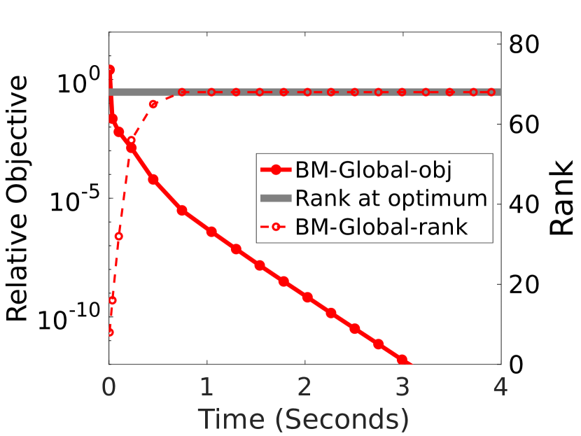
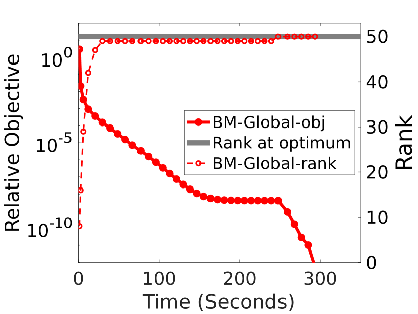
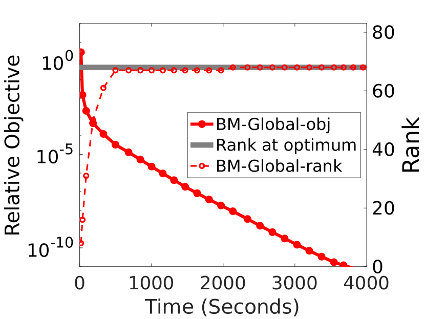
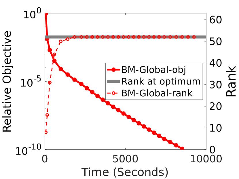
We then show the rank of over iterations of BM-Global In Fig. 1, we use solid lines and dash lines to respectively show the relative objective value and the rank of the iterates of our method. The gray line represents the rank at the optimum . We can see that the rank of increases quickly at first, and eventually stabilizes at the rank of the point of convergence in all cases. Sometimes, the rank remains fixed for a while, then is increased by a small number, and finally stays at the new rank. This is the situation that a safeguard (see the supplementary materials) kicks in to resolve the insufficient rank problem and ensures that the iterates indeed converge to a global optimum. We can also see that when the rank reaches , the relative objective also drops significantly, indicating that finding the right rank is essential in solving Eq. CVX to a high precision.
6.1.3 Comparison between BM-Global and the BM solver alone
We next compare BM-Global with running a BM solver only for Eq. MF. We directly use the solver in our BM phase, namely, the polyMF-SS method of WanLK17a, with their original random start scheme to avoid starting from the origin, which is a known saddle point of Eq. MF. Given any value , their method starts from a randomized and . We favor their method to directly assign as the final rank shown in Table 1, but we emphasize that in real-world applications, finding this will require additional effort in parameter search.
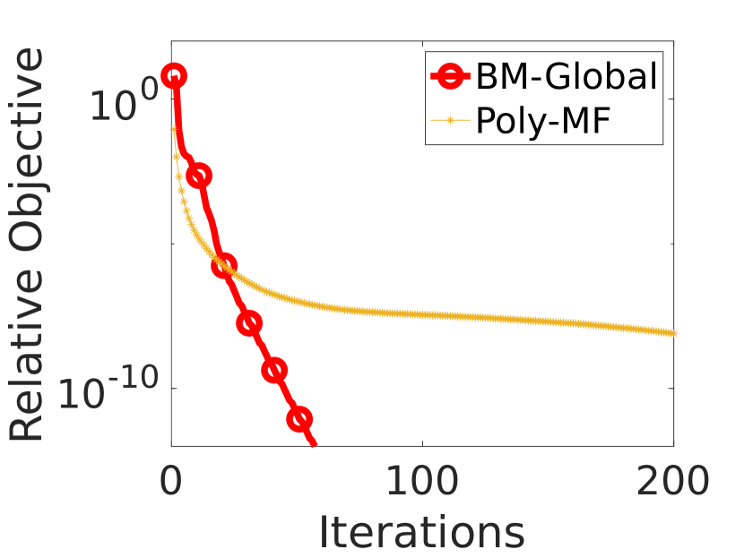
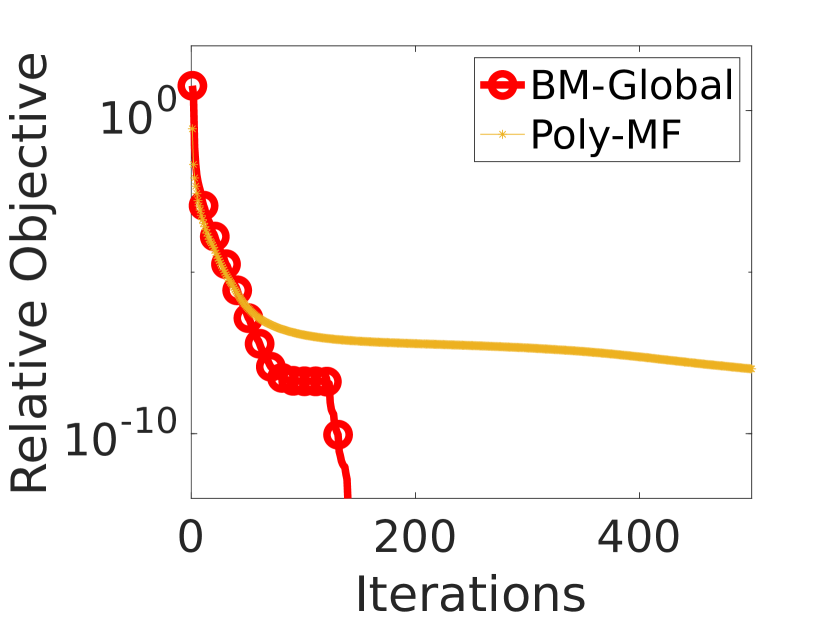
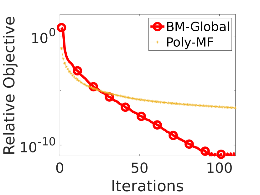
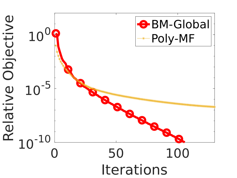
The purpose of this experiment is to show that solving Eq. MF only can get the iterates stuck at saddle points or spurious local minima, while BM-Global can effectively and efficiently escape from such points. Therefore, we consider the relative objective as the only comparison criterion in this experiment. The results of running time and number of iterations are shown in Fig. 2. For the number of iterations, we count either one inexact proximal gradient step or one epoch of polyMF-SS (one sweep through the whole data) as one iteration.
We observe that in terms of iterations, PolyMF-SS has a small early advantage due to the larger starting rank in Eq. BM. But its convergence quickly slows down, suggesting that likely the iterates are attracted to a saddle point or a spurious local minimum that is strictly worse than the global optima. On the other hand, the story in the running time comparison is very different. We see that the higher rank in PolyMF-SS from the beginning on actually increases the time cost per epoch, and thus the early advantage of PolyMF-SS over BM-Global we observed in terms of iterations is not present in the time comparison. Another observation is that in the numerical experiments, the empirical convergence speed of BM-Global is nearly -linear, linking to the case of in Theorem 4.
Overall speaking, BM-Global is as efficient as running a solver for Eq. MF alone, but it provides multiple advantages including the guarantee of convergence to the global optima. Although in this experiment, the stationary points to which the iterates of PolyMF-SS converge seem to be of good enough quality, we have no guarantee that on other datasets, or even on these datasets but with a different , their points of convergence will still be of satisfactory quality.
| Iterations | |||
| Running time | |||
6.1.4 Comparison with existing methods
Now that it is clear our method is advantageous over running a solver for Eq. MF alone, we proceed to compare BM-Global with state of the art for Eq. MC. In particular, we compare BM-Global with the following:
-
•
Active-ALT (HsiO14a): This method alternates between conducting an inexact PG step and solving a lower-dimensional convex subproblem. In the approximate SVD part for inexact PG, HsiO14a use the power method with warmstart from the output of the previous iteration plus some random columns as a safeguard.
-
•
AIS-Impute (YaoKWL18a): An inexact APG method that also uses the power method for approximate SVDs. They use the combination of the outputs of the previous iteration and the iteration preceding it to form the warmstart matrix.
The inexact APG method in (TohY10a) is not included because the underlying APG part is the same as that of AIS-Impute, but their approximate SVD using Lanczos is shown by (YaoKWL18a) to be less efficient.
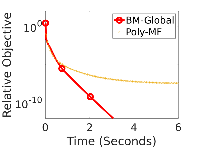
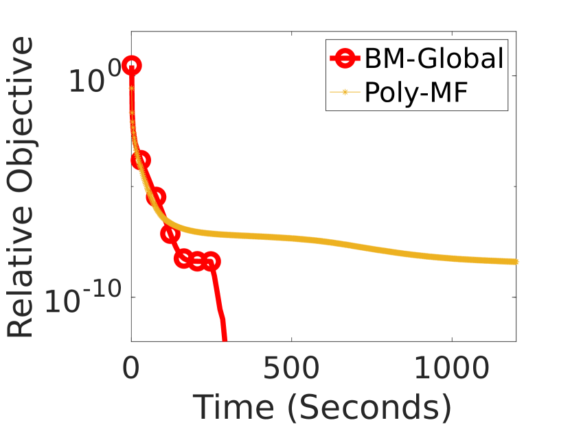
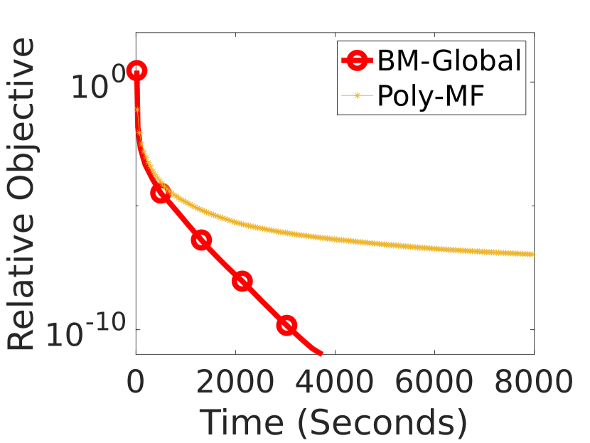
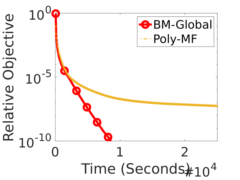
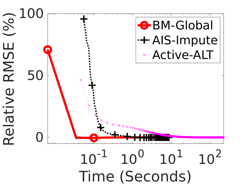
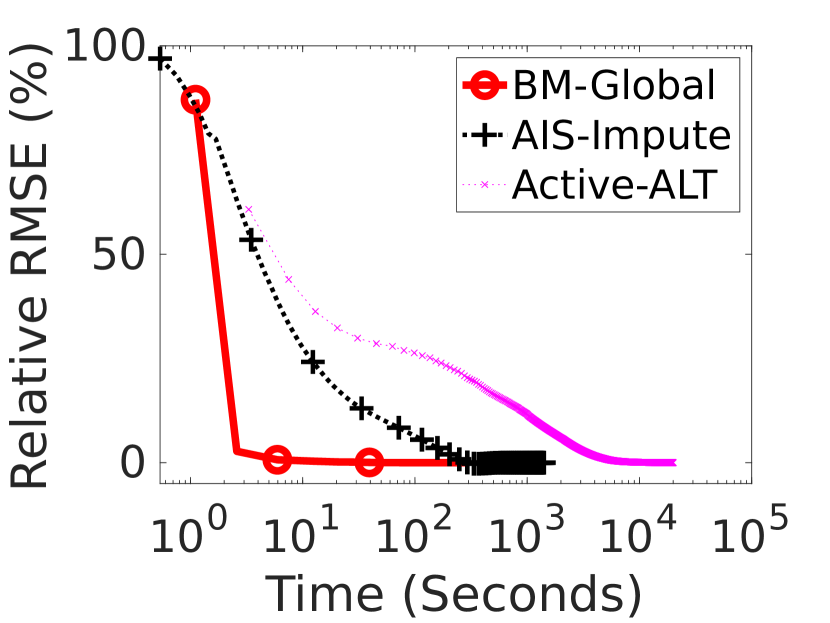
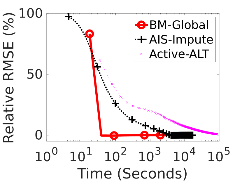
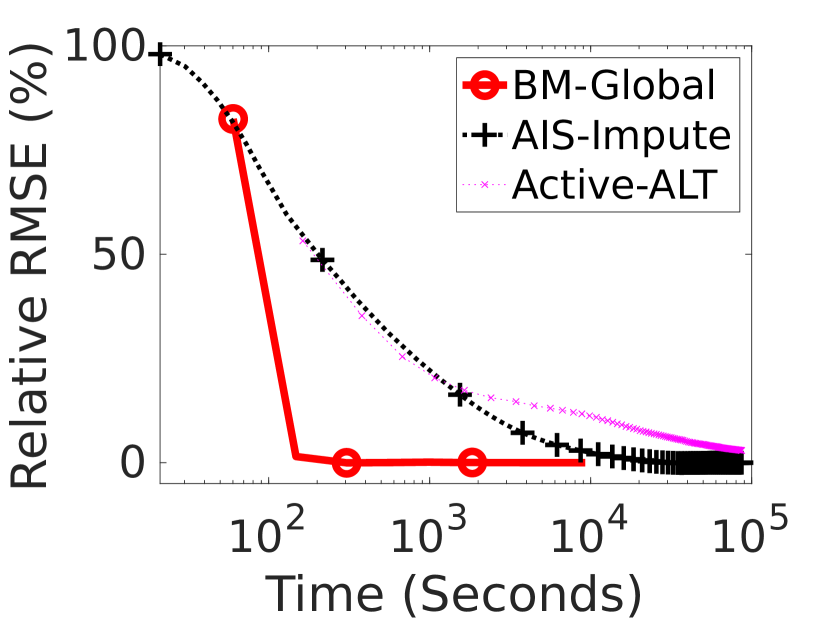
The results of relative objective and relative RMSE are shown in Fig. 3. Note that the running time for relative RMSE in Fig. 3 is in log scale to make the difference legible. Clearly, BM-Global outperforms the state-of-the-art for Eq. MC significantly on both criteria. Particularly, Fig. 3 exemplifies even greater efficiency difference in reaching satisfactory RMSE between BM-Global and existing methods. We can see that the proposed approach is actually magnitudes faster than state-of-the-art in this criterion.
| Relative objective | |||
| Relative RMSE | |||
6.2 Convex QSDP
Next, we consider solving the two applications of QSDP described in Section 5.2. As mentioned before, PG and APG can be applied to solve the problem directly. However, based on our empirical experience, both methods require too many iterations and excessive runtime to reach a reasonably good solution, so their numerical results are excluded here. (Interested readers may refer to the supplementary material for the numerical results of the APG methods.) We hence only compare BM-Global with the efficient and robust QSDP solver, QSDPNAL (li2018qsdpnal).333Avaliable at https://blog.nus.edu.sg/mattohkc/softwares/qsdpnal/.
Regarding the termination conditions, since QSDPNAL computes both primal and dual iterates, its relative KKT residual is computable (see (li2018qsdpnal, Section 5.2) for the definition). Thus, given a specific stopping tolerance tol, QSDPNAL is terminated when the maximum relative KKT residual, denoted by , is less than tol. Moreover, when is large, QSDPNAL may take too much computational time (since it uses full eigendecompositions), so we also cap the running time of QSDPNAL to four hours (initialization overhead excluded) and its maximum number of iterations to . For BM-Global, we terminate it when
In our experiments, we set for both methods.
Recall that the first-order optimality condition for problem Eq. QSDP is given by
Since we are testing problems with that can be handled by QSDPNAL that uses full eigendecompositions, we are in fact able to check whether an approximate solution is optimal numerically, even though this can be time-consuming. Therefore, to compare the quality of the solutions returned by BM-Global and QSDPNAL, we record the relative primal feasibility and the relative optimality, respectively defined as
Experiments for this part are conducted on a Linux PC with an Intel Xeon E5-2650 processor and 96GB memory.
6.2.1 Regularized kernel estimation
We consider problems with dissimilarity measures for collected in (duin2009datasets).444Data available at http://prtools.tudelft.nl/Guide/37Pages/distools.html. In our experiments, the data are scaled to the interval , and the elements of the index set are randomly selected such that . We set for all and .
The results are presented in Table 2. Clearly, both methods are able to compute nearly feasible and low-rank solutions. In terms of the optimality measure, BM-Global is able to solve all the problems with while QSDPNAL fails to do so for one of the problems. In terms of efficiency, we see that BM-Global is faster in most cases, and BM-Global can even be ten times faster than QSDPNAL in the case of the largest instance.
| QSDPNAL | BM-Global | |||||||||
|---|---|---|---|---|---|---|---|---|---|---|
| Name | rnk | Time | rnk | Time | ||||||
| BrainMRI | 124 | 6e-11 | 1e-06 | 1e-06 | 5 | 0.7 | 2e-16 | 5e-07 | 5 | 0.5 |
| protein | 213 | 4e-13 | 4e-06 | 5e-07 | 24 | 4.3 | 5e-11 | 7e-06 | 24 | 1.9 |
| CoilDelftDiff | 288 | 9e-13 | 4e-04 | 9e-07 | 32 | 5.7 | 4e-15 | 5e-08 | 32 | 1.6 |
| coildelftsame | 288 | 9e-14 | 4e-06 | 5e-07 | 32 | 6.7 | 2e-11 | 4e-06 | 32 | 2.3 |
| CoilYork | 288 | 3e-13 | 2e-06 | 4e-07 | 22 | 4.8 | 2e-15 | 7e-06 | 22 | 2.6 |
| Chickenpieces-5-45 | 446 | 4e-13 | 3e-06 | 7e-07 | 27 | 11.5 | 2e-11 | 8e-06 | 28 | 7.6 |
| newgroups | 600 | 8e-13 | 3e-05 | 5e-07 | 81 | 39.6 | 2e-12 | 2e-04 | 83 | 29.6 |
| flowcytodis | 612 | 2e-13 | 4e-06 | 9e-07 | 15 | 14.8 | 1e-12 | 1e-06 | 15 | 13.9 |
| DelftPedestrians | 689 | 3e-12 | 1e-05 | 2e-07 | 69 | 43.7 | 3e-12 | 7e-06 | 69 | 32.8 |
| WoodyPlants50 | 791 | 5e-13 | 1e-05 | 7e-07 | 48 | 44.3 | 9e-13 | 2e-07 | 48 | 78.2 |
| delftgestures | 1500 | 1e-14 | 7e-06 | 5e-07 | 76 | 318.3 | 3e-13 | 2e-06 | 77 | 390.1 |
| zongker | 2000 | 2e-11 | 1e-02 | 8e-07 | 264 | 1000.2 | 6e-12 | 1e-04 | 267 | 665.6 |
| polydish57 | 4000 | 2e-12 | 1e-05 | 5e-07 | 100 | 3508.9 | 7e-15 | 3e-05 | 101 | 1765.2 |
| polydism57 | 4000 | 1e-12 | 5e-04 | 8e-07 | 25 | 3286.4 | 1e-16 | 2e-07 | 26 | 305.0 |
6.2.2 Molecular conformation
In this experiment, we consider the molecules from the Protein Data Bank (see https://www.rcsb.org/) with given noisy and sparse distance data to simulate distances measurable by nuclear magnetic resonance (NMR) experiments. For each molecule, if the distance between two compatible atoms is less than 6Å( cm), then the distance can be measured by the NMR experiment; otherwise, we assume that no information is known for this pair. To simulate the sparse set of distances measurable by the NMR experiment, among all the pairwise distances less than 6Å, we select 25% of them to generate our index set . We then add in additional noise to the observed data as follows. Let be a given noise level and be the exact distance between atom and atom for , we sample two independent random variables from the normal distribution and define
Then, the input distances are set as . Given , we set . Moreover, we let . In our tests, we set . To measure the accuracy of the estimated positions, we record the root mean square deviation (RMSD):
where is the estimated position and is the actual position. Note that a smaller RMSD means a better estimation, and an RMSD of less than 2Å is considered to be good in molecular conformation.
The computational results are presented in Table 3. It is clear that both methods return nearly feasible solutions. However, we can see that BM-Global outperforms QSDPNAL in all other measures. In particular, QSDPNAL often returns solutions with a large suboptimality measure, and those solutions tend to be of a higher rank and give a larger RMSD. On the other hand, the solutions returned by BM-Global are always of low rank with very small RMSD. Moreover, by the presented computational time, we see that BM-Global is much more efficient than QSDPNAL, and its generated solutions are also often much more accurate.
The results in this and the previous subsections also suggest that the numerical performance of QSDPNAL may depend on the sign of while BM-Global is robust with respect to parameter selection of .
| QSDPNAL | BM-Global | |||||||||||
|---|---|---|---|---|---|---|---|---|---|---|---|---|
| Name | rnk | RMSD | Time | rnk | RMSD | Time | ||||||
| 1PBM | 126 | 1e-12 | 9e-09 | 7e-07 | 10 | 2.7 | 25.0 | 1e-13 | 3e-08 | 10 | 2.7 | 2.0 |
| 1AU6 | 161 | 3e-12 | 3e-08 | 8e-07 | 12 | 1.1 | 34.1 | 1e-13 | 2e-08 | 12 | 1.1 | 4.0 |
| 1PTQ | 402 | 2e-12 | 4e-08 | 8e-07 | 14 | 0.7 | 358.6 | 2e-16 | 3e-08 | 15 | 0.7 | 13.9 |
| 1CTF | 487 | 3e-12 | 8e-09 | 9e-07 | 13 | 0.7 | 570.3 | 1e-15 | 3e-08 | 15 | 0.8 | 18.0 |
| 1HOE | 558 | 1e-12 | 2e-08 | 1e-06 | 15 | 0.8 | 899.6 | 7e-16 | 1e-08 | 16 | 0.7 | 32.7 |
| 1LFB | 641 | 5e-13 | 1e-08 | 3e-06 | 15 | 1.2 | 2739.5 | 4e-16 | 3e-08 | 17 | 1.5 | 25.5 |
| 1PHT | 666 | 2e-13 | 8e-08 | 1e-06 | 15 | 1.1 | 2091.9 | 8e-16 | 4e-08 | 18 | 1.4 | 36.3 |
| 1F39 | 767 | 4e-12 | 2e-08 | 3e-06 | 17 | 1.3 | 3230.1 | 8e-16 | 2e-08 | 20 | 0.8 | 44.0 |
| 1DCH | 806 | 7e-13 | 2e-08 | 4e-06 | 18 | 1.6 | 3897.0 | 3e-16 | 4e-09 | 18 | 1.1 | 41.8 |
| 1HQQ | 891 | 6e-13 | 2e-08 | 4e-06 | 17 | 2.7 | 5089.2 | 7e-16 | 1e-08 | 21 | 1.0 | 43.5 |
| 1POA | 914 | 1e-12 | 2e-08 | 4e-06 | 16 | 2.1 | 4734.1 | 1e-15 | 4e-09 | 19 | 1.1 | 65.4 |
| 1AX8 | 1003 | 6e-13 | 2e-08 | 4e-06 | 17 | 3.0 | 6397.0 | 2e-16 | 4e-09 | 18 | 1.7 | 61.1 |
| 1TJO | 1394 | 5e-13 | 2e-08 | 5e-06 | 21 | 12.3 | - | 2e-15 | 9e-10 | 29 | 2.3 | 77.4 |
| 1RGS | 2015 | 3e-12 | 8e-08 | 6e-06 | 39 | 16.1 | - | 1e-15 | 4e-09 | 31 | 2.3 | 168.8 |
| 1TOA | 2138 | 9e-12 | 2e-07 | 8e-06 | 49 | 16.8 | - | 2e-15 | 2e-09 | 31 | 1.0 | 142.4 |
| 1KDH | 2846 | 3e-11 | 2e-06 | 2e-05 | 150 | 21.9 | - | 5e-16 | 2e-09 | 40 | 2.1 | 199.1 |
| 1NFG | 3501 | 2e-12 | 3e-05 | 1e-04 | 325 | 21.2 | - | 3e-15 | 3e-09 | 43 | 1.0 | 275.8 |
| 1BPM | 3672 | 1e-12 | 5e-05 | 2e-04 | 396 | 23.8 | - | 5e-17 | 8e-10 | 40 | 1.4 | 438.6 |
| 1MQQ | 5510 | 1e-14 | 4e-04 | 1e-03 | 911 | 26.0 | - | 2e-15 | 1e-09 | 61 | 1.3 | 947.1 |
7 Conclusions
In this work, we proposed an efficient algorithm BM-Global for solving the low-rank matrix optimization problem. We utilized both the efficiency from a smooth objective of the Burer-Monteiro decomposition approach and the convexity and partial smoothness of the nuclear-norm-regularized convex form to obtain a highly efficient algorithm with sound theoretical guarantees. Extensive numerical experiments showed that our proposed algorithm outperforms state-of-the-art for low-rank matrix optimization.
Acknowledgement
This work was partially done when Lee was visiting the Department of Mathematics at the National University of Singapore. Lee’s research was supported in part by NSTC of Taiwan grants 109-2222-E-001-003-MY3 and 111-2628-E-001-003-, and Academia Sinica grant AS-GCS-111-M05. Toh’s research is supported by the Ministry of Education, Singapore, under its Academic Research Fund Tier 3 grant call (MOE-2019-T3-1-010).
References
Part Supplementary Materials
Appendix I Implementation Details
I.1 Matrix Completion
We now describe our implementation details of BM-Global that are tailored for the matrix completion problem. In particular, we will discuss the mechanism for deciding in Eq. 12, the algorithm for obtaining the approximate eigendecomposition using only matrix-vector products, details of the safeguard to ensure in Eq. 12, initialization strategy for , the solver for Eqs. BM-nuclear and BM-PSD, and the degree of parallelism of our algorithm.
To avoid redundancy, we focus on the case of Eq. BM-nuclear in this section, and keep in our mind that it can be easily adapted to the case of Eq. BM-PSD by straightforward changes from SVDs to eigendecompositions.
I.1.1 Approximate SVD
Let us denote
| (I.1) |
For the proximal operation Eq. 4, since by our assumption, it is cheaper to compute an approximate eigendecomposition of (instead of ) to get
| (I.2) |
for some with and some orthogonal for a given rank . The notation denotes the element-wise square. Note that here we have removed the eigenvectors corresponding to the eigenvalue as it does not affect the product matrix. We then conduct an exact SVD on (whose calculation can be done without forming or explicitly) to obtain
| (I.3) |
with cost , which is much cheaper than SVD for when . The approximate SVD of is then obtained through
| (I.4) |
where coincides with the one we used in Eqs. 10 and 11. Clearly, and are both orthonormal, so this is indeed a valid SVD for the matrix
The inexact proximal gradient step is then finished as
| (I.5) |
Note that we only store but do not explicitly form . Here we slightly abuse the notation to let denote only the coordinates of the thresholded vector that have a nonzero value, and let and contain only the columns corresponding to these values to save spatial and computational cost.
I.1.2 An Efficient Algorithm for Approximate Eigendecompositions Using Only Matrix-Matrix Products
As mentioned before, forming and is prohibitively expensive. Therefore, for computing Eq. I.2, we need to rely on iterative methods that only require evaluating matrix multiplications involving and , so that we can utilize the decomposition of as well as the structured assumption of made in Section 1. A highly efficient and robust approach is the limited memory block Krylov subspace method (LmSVD) proposed by (LiuWZ13a); see also the references therein for other popular algorithms. LmSVD is an extension of the classic simple subspace iteration (SSI) method for computing the extremal eigenvalues and eigenvectors that extends from the renowned power method (i.e., ). For any initial guess for right-singular vectors , the SSI method computes the new iterates via
| (I.6) |
where extracts an orthonormal basis for the range space of the given matrix , and is the iteration counter for SSI. For the ease of description, we abstract the operation for an input as a self-adjoint semidefinite operator . Note that in each iteration of SSI, one needs to perform two matrix multiplications (one for and the other for ) and one orthonormalization that cost and flops, respectively. In our case, suppose that , then the main computational bottleneck is the matrix products. Therefore, LmSVD tries to accelerate the practical convergence via cutting down the total number of iterations to reduce such matrix products without incurring additional heavy computation. To achieve this goal, LmSVD finds the next iterate via replacing in Eq. I.6 with an improved candidate via solving the following constrained optimization problem:
| (I.7) |
where the subspace is selected as
for some pre-specified . Let and
then if and only if there exists such that
| (I.8) |
Direct computation then shows that Eq. I.7 is equivalent to
| (I.9) |
However, the matrix may be rank deficient to cause numerical issues in solving Eq. I.9. To resolve this issue, LmSVD replaces with an orthonormal basis of . To extract such a basis, since (i.e., the first block in matrix ) always has a full column rank, LmSVD first projects the remaining blocks in to to form
| (I.10) |
and then consider its orthonormalization. We denote the eigendecomposition of by
for matrices with orthonormal and diagonal. Clearly, if is nonsingular,
| (I.11) |
is an orthonormal basis of . In practice, we can drop those columns of that correspond to nearly zero eigenvalues of . Moreover, there may exist columns of whose norms are nearly zero. To stabilize the numerical computation, one might also want to drop these columns. From here on, we always assume that , for some , forms an orthonormal basis of and it is obtained via performing the above two trimming procedures to the matrix in Eq. I.11.
After knowing an orthonormal basis i of , we then express any as
for some . The above expression then yields the following optimization problem to be solved at each iteration of LmSVD.
| (I.12) |
where . The solution for problem Eq. I.12 is nothing but the leading eigenvectors of the matrix . Therefore, we can compute the full spectral decomposition of to get and the computational cost is acceptable provided that and are small. The overall algorithm of LmSVD is summarized in Algorithm 2.
We emphasize that LmSVD has an efficient and robust official implementation by (LiuWZ13a).555Available at https://www.mathworks.com/matlabcentral/fileexchange/46875-lmsvd-m. In the present work, we borrow most parts of the implementation of (LiuWZ13a) but impose some minor modifications to adapt for our purposes. First, as we shall see in the following subsection, instead of using a randomly generated initial point , we use a more sophisticated initialization scheme. Second, the implementation of (LiuWZ13a) terminates by following a two-level strategy, but in our implementation, we simply terminate the algorithm as long as the difference between the eigenvalues of and is small.
I.1.3 Ensuring Sufficient Precision in the Proximal Operation
We notice that Eq. I.5 suggests that all entries in smaller than the threshold as well as their corresponding columns of and do not contribute to the calculation of , so we just need to compute the entries not truncated by the proximal operation. Therefore, if , ideally we just need to compute the first eigenvalues in our approximate eigendecomposition at the th iteration of proximal gradient. On the other hand, to ensure that we are recovering a global solution of Eq. CVX, it is necessary to check that the ranks of the iterates are large enough so that we do not get stuck at an approximation of with an insufficient rank. To safeguard that our algorithm converges to a global optimum, or more explicitly, to make in Eq. 12 decrease to fast enough (see Section 4), we want to ensure that eventually the smallest eigenvalue we obtain will be truncated out, so that we can be certain that all eigenvalues/eigenvectors that contribute to the computation of have already been obtained. Therefore, we will need a mechanism to adaptively adjust the rank of . As the decrease of the rank is achieved by the truncation in the proximal operation, following our usage of LmSVD described in the previous subsection, what we need is a way to make the initial guess input to LmSVD have a rank sufficiently higher than that of and .
As noted in Lemma 1, we know that the output of approximately solving Eq. BM-nuclear should be close to the singular vectors of (up to column-wise scaling). Moreover, when and are close to a global optimum , we expect that will be close to and thus also to and , so the SVD of is also expected to be close to that of and . We therefore use from Eq. I.4 and from the output of the BM phase to form
| (I.13) |
as the base of our the warmstart input to the approximate eigendecomposition in obtaining from . If the BM phase is not entered or does not produce any change in the iterate, we use
| (I.14) |
instead. To further guarantee that in Eq. 12, we need to ensure that the rank of is sufficiently large, and that will approach the singular vectors corresponding to the singular values not truncated out. Ideally, we hope that the output of our approximate eigendecomposition will be exactly all the eigenvalues or singular values that are retained nonzero, plus the largest one that is truncated out in Eq. 4. Therefore, we add in one column with randomness to whenever the rank of and are the same (namely, the rank has stopped increasing) and there is at most one eigenvalue truncated out in the inexact proximal gradient step at the th iteration. The idea is that the case of truncating only one eigenvalue is the ideal scenario we want and we want the next iteration to still have one eigenvalue to truncate as the safeguard, while if no truncation happened, then we should continue increasing the rank. Utilizing this idea, we retain the singular vector that corresponds to the largest truncated singular value in the latest iteration where such a truncation took place, and compute its projection to . (It is possible and acceptable that .) The warmstart input is finally formed by
| (I.15) |
where is a random vector and is a sequence such that .
When the rank of and are the same, it means no truncation took place in the proximal operation, and we view this as that the maintained has been added to as a column in the next iteration when we call LmSVD to compute an approximate eigendecomposition. In this situation, we then seek the eigenvector that corresponds to the next eigenvalue truncated as our new . When there is no more such vectors available, we simply add in a unit random vector that is orthogonal to the columns of .
Here we provide further explanations to our design above. Assume that the eigenvalues in the exact eigendecomposition of are , is the set of those eigenvalues that will not become zero after the truncation in Eq. I.5, and are those that will become zero after the truncation in Eq. I.5. To cope with pathological cases in which some eigenvectors corresponding to some and some corresponding to are obtained, we inject noise to so that during the procedure of Algorithm 2, it will approach an eigenvector that corresponds to some value in instead of getting stuck at an eigenvector that will be truncated out. (Analysis of the classical SSI suggests that approaches the leading eigenvectors as long as no column is exactly a multiple of an eigenvector that corresponds to an eigenvalue with a smaller absolute value.) On the other hand, when we are close to an optimal solution of Eq. CVX, and the eigenvectors corresponding to are all identified or well-approximated, it is natural that we do not want to add in much noise in the initialization of Algorithm 2, as such noise will decelerate the convergence of Algorithm 2. Therefore, in our design, we only add with noise to when or , namely when no truncation happened or when only one vector is truncated. In the latter case, adding to is for the purpose of making contain one eigenvector that is likely to be truncated, so that we can still have the safeguard for ensuring that we have found the correct rank in the approximate eigendecomposition. We then decrease the level of noise by a certain factor whenever . That is, when exactly only one eigenvalue is truncated. This corresponds to Eq. I.15. For the noise level , in our implementation, we start with so that the noise will not dominate , and whenever we need to decrease the significance of the noise, we just let , and otherwise we assign .
I.1.4 Initialization
It can be clearly seen that the point of origin is a saddle point of Eq. BM-nuclear, and this is also the case for many other popular problems that has the form of Eq. BM. Therefore, it is essential to have an effective way to initialize , or equivalently , in Algorithm 1. Existing methods for Eq. BM usually take a random initialization, but such approaches often lead to an unideal initial objective even worse than using . Moreover, it is hard to decide what is an appropriate value for the initial rank – too large the rank takes longer running time, but too small the rank might lead to slow convergence at the early stage. The most straightforward idea would be to conduct one (inexact) proximal gradient step from the origin, but the difficulty is that we will be in lack of a warmstart matrix for the approximate eigendecomposition in Algorithm 2, and we still need to decide the rank of this matrix.
To get a good initialization for , we follow the recent developments in randomized numerical linear algebra by (HalMT11a; Mar19a) to combine the HMT method (HalMT11a) with the Nyström method (Nys30a). We imagine that our starting point is actually , and then conduct one step of inexact proximal gradient from there with the fixed stepsize to initialize . Regarding the approximate SVD for
we describe how to obtain the eigendecomposition of . Given the initial rank , we start with a random matrix whose entries are independently and identically distributed as the standard normal distribution. Then we conduct
as in the HMT method, and use this as the sketching matrix in the Nyström method to consider the approximation
| (I.16) |
where for any matrix , is its pseudo inverse. The approximation matrix here is not really explicitly computed, but only serves as an intermediate variable for our further process. Clearly, , and thanks to the randomness from and therefore , with high probability we have . We can then compute the exact eigendecomposition for by separately considering and . As long as is small, the computation of both and is affordable under our assumption of efficient matrix-matrix products involving , and so is the calculation of the pseudo inverse that costs . For obtaining the exact eigendecomposition of , we first compute a QR decomposition of
where is an orthonormal matrix and is upper triangular. We then obtain the eigendecomposition of
which costs only in both forming the matrix on the left-hand side and calculating its eigendecomposition, as the matrices involved are all by . When , this cost is negligible in comparison to other steps. The eigendecomposition of is then obtained by setting to get in the right-hand side of Eq. I.2. The next steps for initializing then directly follow the procedure of Eqs. I.3, I.4 and I.5.
The remaining issue is to decide the rank for . The most naive idea is to set so that all computation in the initialization is of the lowest possible overhead. However, in this case, we will not be able to fully exploit the multicore advantage of modern computing devices. We therefore set the initial to be the number of cores we can use, so that all the matrix-matrix computation of this step can be fully parallelized without increasing the overhead for initialization.
I.1.5 Solver for Eq. BM-nuclear
The step of optimizing Eq. BM-nuclear relies on an off-the-shore solver, and to obtain the best efficiency, the choice should be application-dependent. As we aim for large-scale problems and wish to fully exploit multicore parallelization ubiquitous in modern computers, we will use methods that efficiently utilize multiple computational cores. For Eq. BM-nuclear, as the objective is smooth, many algorithms are available for this choice, ranging from asynchronous, low-order ones to synchronous, high-order approaches. For the low-order ones, we note that since each row of affects different entries in , one can update multiple rows simultaneously if is separable, and the same argument applies to the update of as well. Therefore, as long as is no fewer than the number of cores, we should be able to enjoy full parallelism. For problems like Eq. MF, many efficient algorithms such as those by (YuHSD14a; ZhuCJL13a; WanLK17a) are readily available. On the other hand, for Eq. BM-PSD, the property of the constraint set will limit our choices for the solver. In most applications, however, the constraint can be formulated as a smooth manifold for , and one can utilize efficient manifold optimization approaches for such problems; see, for example, (AbsMS09a; manopt). The major computation in such manifold optimization approaches is usually the computation of the Riemannian gradient and the Hessian-vector products, which are by nature parallelizable.
I.1.6 Parallelism
A key to cope with large-scale problems in modern computing environments is to utilize multicore parallelization. Although inherently the bottleneck of Algorithm 2, Eq. I.6, can be highly parallelized, in practice usually the parallelism is low as this operation is data-heavy but not computation-heavy, so higher parallelism is hindered by the memory bandwidth. On the other hand, solvers for Eq. BM-nuclear tend to be more computationally intensive, so they can often achieve better parallelism, by utilizing all cores available, than solvers for Eq. CVX. By switching to the BM phase, our algorithm hence exploits better parallelism than state of the art for Eq. CVX. The initial rank in the previous subsection is also selected to fully exploit the advantage of multiple cores from the beginning on.
I.2 Quadratic SDP
I.2.1 The BM formulations for the RKE problem and the molecular conformation problem.
For the RKE problem and the molecular conformation problem, the corresponding factorized problem is given as
| (I.17) |
The gradient of this function is
For any given , the Hessian operator of performed on can be computed as
I.2.2 Implementation Details
Recall that for a given problem size , Algorithm 1 iterates on a low-rank matrix with dynamically adjusted. In our experiment, we choose the initial as
Given , we then run APG for iterations with this rank constraint to generate an initial point . When applying the APG method, we never form the matrix and use only eigendecompositions with rank . In particular, we use MATLAB’s built-in eigs subroutine to compute the largest eigenpairs. After the initialization stage, at the -th iteration of Algorithm 1, we first apply the Manopt solver to solve the factorized problem Eq. I.17 with the initial point to compute a matrix . Using , we then perform one inexact PG step with an approximate eigendecomposition with fixed step size . If all the computed eigenvalues are positive, then it is highly possible that the current rank is too small. In this case, we set . Otherwise, we set as the number of positive eigenvalues returned by eigs.
I.2.3 The accelerated proximal gradient method
Since we utilize the APG method for the initialization of BM-Global for Eq. QSDP, for completeness, we provide a concise description of the APG method in Algorithm 3. To perform the projection for Eq. QSDP through Lemma 7, we use the eig subroutine in MATLAB. (Note that the PG method is equivalent to setting in Algorithm 3.)
Appendix II Additional Experimental Details and More Experiments
II.1 The SpaRSA variant for Matrix Completion
It is known that the convergence speed of standard PG could be slow, thus we also considered following (WriNF09a) to use the Barzilai-Borwein (BB) initialization (barzilai1988two) with linesearch to decide the step size to accelerate the practical convergence of the convex lifting step. Given , we first compute
| (II.1) |
But different from (WriNF09a), our backtracking linesearch does not search for an that gives sufficient descent. Instead, given , we find the smallest nonnegative integer such that satisfies Eq. 13 or Eq. 14.
In our scenario, we only have the factorized form for each but not the iterate itself, so we use the following formula to calculate the numerator of Eq. II.1, which is also used as the last term in Eq. 13.
| (II.2) |
Similar calculation is also applied to compute the denominator of Eq. II.1. If and , the cost of computing Eq. II.2 is .
II.2 Experimental Details of Section 6.1.1
We report the required running time for making the relative objective smaller than for both the fixed-step variant and the SpaRSA variant of our algorithm. The algorithms are terminated either when they have reached or when they have conducted inexact proximal gradient steps. The results are shown in Tables (IV) and (V).
Aside from the selection of and made in the main paper for the fixed-step variant, for SpaRSA, we also see that and is still robust and we thus use this setting for SpaRSA from now on.
| SpaRSA | 5.4e0 | 1.1e0 | 1.2e0 | 1.4e0 | 1.5e0 | 1.6e0 | 1.7e0 | 1.8e0 | |
|---|---|---|---|---|---|---|---|---|---|
| 1.4e0 | 1.3e0 | 1.8e0 | 1.7e0 | 1.9e0 | 2.1e0 | 2.4e0 | 2.6e0 | ||
| 1.1e0 | 1.1e0 | 1.1e0 | 1.2e0 | 1.2e0 | 1.2e0 | 1.3e0 | 1.3e0 | ||
| 1.3e0 | 1.0e0 | 1.1e0 | 1.2e0 | 1.6e0 | 1.7e0 | 1.8e0 | 1.8e0 | ||
| 1.0e0 | 1.1e0 | 1.3e0 | 1.3e0 | 1.4e0 | 1.5e0 | 1.6e0 | 1.7e0 | ||
| 1.2e0 | 1.0e0 | 1.2e0 | 1.3e0 | 1.4e0 | 1.6e0 | 1.7e0 | 2.0e0 | ||
| 1.2e0 | 1.5e0 | 1.5e0 | 1.7e0 | 1.9e0 | 2.1e0 | 2.3e0 | 2.5e0 | ||
| 1.5e0 | 1.2e0 | 1.1e0 | 1.2e0 | 1.2e0 | 1.3e0 | 1.3e0 | 1.4e0 | ||
| 1.2e0 | 1.3e0 | 1.3e0 | 1.4e0 | 1.5e0 | 1.6e0 | 1.7e0 | 1.7e0 | ||
| 1.3e0 | 1.2e0 | 1.3e0 | 1.4e0 | 1.5e0 | 1.6e0 | 1.8e0 | 1.9e0 | ||
| SpaRSA | 1.2e1 | 3.7e0 | 4.9e0 | 5.0e0 | 5.5e0 | 5.8e0 | 7.0e0 | 7.1e0 | |
| 3.6e0 | 6.3e0 | 4.3e0 | 4.9e0 | 4.7e0 | 5.8e0 | 5.3e0 | 5.6e0 | ||
| 3.2e0 | 3.6e0 | 4.2e0 | 4.1e0 | 4.5e0 | 4.8e0 | 5.2e0 | 5.7e0 | ||
| 3.3e0 | 3.2e0 | 3.2e0 | 3.4e0 | 3.6e0 | 3.8e0 | 4.1e0 | 4.3e0 | ||
| 3.3e0 | 3.7e0 | 3.5e0 | 4.4e0 | 4.5e0 | 4.8e0 | 5.1e0 | 5.4e0 | ||
| 4.4e0 | 3.7e0 | 4.9e0 | 5.4e0 | 6.4e0 | 7.1e0 | 7.7e0 | 8.4e0 | ||
| 4.4e0 | 3.8e0 | 4.2e0 | 4.6e0 | 5.1e0 | 5.2e0 | 5.5e0 | 5.7e0 | ||
| 4.4e0 | 3.8e0 | 4.1e0 | 4.6e0 | 4.9e0 | 5.2e0 | 5.6e0 | 6.0e0 | ||
| 5.0e0 | 3.6e0 | 3.6e0 | 3.9e0 | 4.0e0 | 4.3e0 | 4.5e0 | 4.7e0 | ||
| 4.9e0 | 4.1e0 | 4.2e0 | 4.5e0 | 4.5e0 | 4.8e0 | 5.3e0 | 5.3e0 | ||
| SpaRSA | 1.6e1 | 7.4e0 | 8.1e0 | 7.9e0 | 9.6e0 | 9.1e0 | 1.0e1 | 1.2e1 | |
| 1.1e1 | 8.9e0 | 7.7e0 | 8.2e0 | 8.4e0 | 9.4e0 | 9.2e0 | 9.0e0 | ||
| 1.0e1 | 7.0e0 | 7.2e0 | 7.2e0 | 7.1e0 | 7.3e0 | 7.8e0 | 8.6e0 | ||
| 9.0e0 | 7.6e0 | 7.1e0 | 7.0e0 | 7.4e0 | 7.9e0 | 7.6e0 | 7.5e0 | ||
| 1.1e1 | 7.8e0 | 6.2e0 | 6.8e0 | 6.9e0 | 7.3e0 | 6.9e0 | 7.9e0 | ||
| 1.2e1 | 6.8e0 | 8.0e0 | 7.7e0 | 8.8e0 | 9.3e0 | 1.0e1 | 1.0e1 | ||
| 1.7e1 | 6.9e0 | 7.1e0 | 7.1e0 | 7.8e0 | 7.8e0 | 8.4e0 | 8.7e0 | ||
| 1.4e1 | 7.2e0 | 6.9e0 | 7.9e0 | 7.8e0 | 8.0e0 | 8.6e0 | 8.5e0 | ||
| 1.3e1 | 7.7e0 | 6.9e0 | 7.4e0 | 7.7e0 | 8.0e0 | 8.6e0 | 8.8e0 | ||
| 1.7e1 | 7.6e0 | 6.5e0 | 7.1e0 | 7.4e0 | 7.9e0 | 8.4e0 | 8.3e0 | ||
| SpaRSA | 5.7e1 | 5.2e1 | 4.1e1 | 4.6e1 | 5.1e1 | 5.4e1 | 5.7e1 | 6.0e1 | |
|---|---|---|---|---|---|---|---|---|---|
| 2.0e0 | 1.4e0 | 7.0e1 | 6.8e1 | 5.7e1 | 5.6e1 | 4.9e1 | 9.5e1 | ||
| 3.8e0 | 2.4e0 | 1.6e0 | 1.6e0 | 9.1e1 | 9.3e1 | 8.0e1 | 5.8e1 | ||
| 4.1e0 | 2.9e0 | 2.3e0 | 1.7e0 | 1.3e0 | 1.3e0 | 7.7e1 | 7.4e1 | ||
| 3.9e0 | 2.6e0 | 2.1e0 | 1.5e0 | 1.5e0 | 1.4e0 | 1.1e0 | 9.7e1 | ||
| 7.8e1 | 4.5e1 | 4.4e1 | 4.3e1 | 5.3e1 | 5.7e1 | 6.0e1 | 6.3e1 | ||
| 1.6e0 | 8.0e1 | 5.7e1 | 5.2e1 | 4.5e1 | 4.9e1 | 5.2e1 | 5.5e1 | ||
| 2.2e0 | 1.4e0 | 1.0e0 | 1.1e0 | 8.1e1 | 7.7e1 | 5.3e1 | 5.6e1 | ||
| 2.5e0 | 1.6e0 | 1.3e0 | 1.3e0 | 1.0e0 | 9.4e1 | 6.6e1 | 6.3e1 | ||
| 2.8e0 | 1.9e0 | 1.6e0 | 1.4e0 | 1.1e0 | 1.1e0 | 8.2e1 | 8.1e1 | ||
| SpaRSA | 2.4e0 | 2.2e0 | 1.9e0 | 1.7e0 | 1.6e0 | 1.6e0 | 1.7e0 | 1.7e0 | |
| 4.6e0 | 4.2e0 | 3.2e0 | 2.4e0 | 2.1e0 | 1.8e0 | 1.7e0 | 1.6e0 | ||
| 7.0e0 | 5.2e0 | 4.4e0 | 3.5e0 | 2.9e0 | 2.7e0 | 2.7e0 | 2.4e0 | ||
| 7.6e0 | 5.9e0 | 4.8e0 | 4.0e0 | 3.5e0 | 3.1e0 | 3.0e0 | 2.6e0 | ||
| 7.2e0 | 5.8e0 | 4.6e0 | 4.2e0 | 3.6e0 | 3.4e0 | 3.3e0 | 2.9e0 | ||
| 2.4e0 | 2.0e0 | 1.7e0 | 1.6e0 | 1.6e0 | 1.8e0 | 2.0e0 | 2.2e0 | ||
| 3.4e0 | 2.7e0 | 2.1e0 | 1.9e0 | 1.8e0 | 1.7e0 | 1.7e0 | 1.7e0 | ||
| 4.3e0 | 3.4e0 | 2.8e0 | 2.7e0 | 2.3e0 | 2.1e0 | 2.1e0 | 1.9e0 | ||
| 4.9e0 | 3.8e0 | 3.2e0 | 3.0e0 | 2.6e0 | 2.4e0 | 2.2e0 | 2.1e0 | ||
| - | 4.2e0 | 3.5e0 | 3.2e0 | 2.8e0 | 2.6e0 | 2.5e0 | 2.3e0 | ||
| SpaRSA | 4.6e0 | 3.8e0 | 3.5e0 | 3.3e0 | 3.4e0 | 3.2e0 | 2.9e0 | 2.9e0 | |
| 7.0e0 | 6.6e0 | 5.3e0 | 4.2e0 | 3.8e0 | 3.4e0 | 3.2e0 | 3.0e0 | ||
| 9.9e0 | 7.5e0 | 6.8e0 | 5.4e0 | 4.6e0 | 4.5e0 | 4.3e0 | 4.0e0 | ||
| - | 8.8e0 | 7.3e0 | 6.2e0 | 5.4e0 | 5.1e0 | 4.7e0 | 4.2e0 | ||
| - | 8.8e0 | 7.3e0 | 6.2e0 | 5.6e0 | 5.5e0 | 5.0e0 | 4.6e0 | ||
| 5.5e0 | 3.7e0 | 3.3e0 | 3.1e0 | 3.0e0 | 3.0e0 | 3.1e0 | 3.4e0 | ||
| 5.7e0 | 4.5e0 | 3.6e0 | 3.4e0 | 3.2e0 | 3.2e0 | 3.1e0 | 3.0e0 | ||
| - | 5.2e0 | 4.3e0 | 4.3e0 | 3.7e0 | 3.6e0 | 3.4e0 | 3.3e0 | ||
| - | 5.8e0 | 4.8e0 | 4.5e0 | 4.1e0 | 3.9e0 | 3.7e0 | 3.5e0 | ||
| - | - | 5.3e0 | 4.9e0 | 4.4e0 | 4.2e0 | 3.9e0 | 3.7e0 | ||
II.3 Comparison with the SpaRSA variant for Matrix Completion
In this subsection, we present experimental results with the SpaRSA variant. The results are shown in Fig. (IV). As expected, this variant is faster than the fixed-step variant in terms of iterations, although the difference is minor. On the other hand, it is significantly slower in terms of the real running time. The likely reason is the possible additional approximate SVDs executed in the backtracking procedure, while the inexact PG step in our algorithm is not the major contributor to the objective decrease, so the improvement in the convergence speed of this part cannot counterbalance the corresponding additional cost.
| Iterations | |||
| Running time | |||
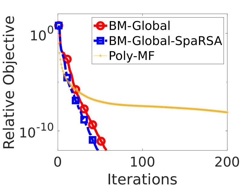
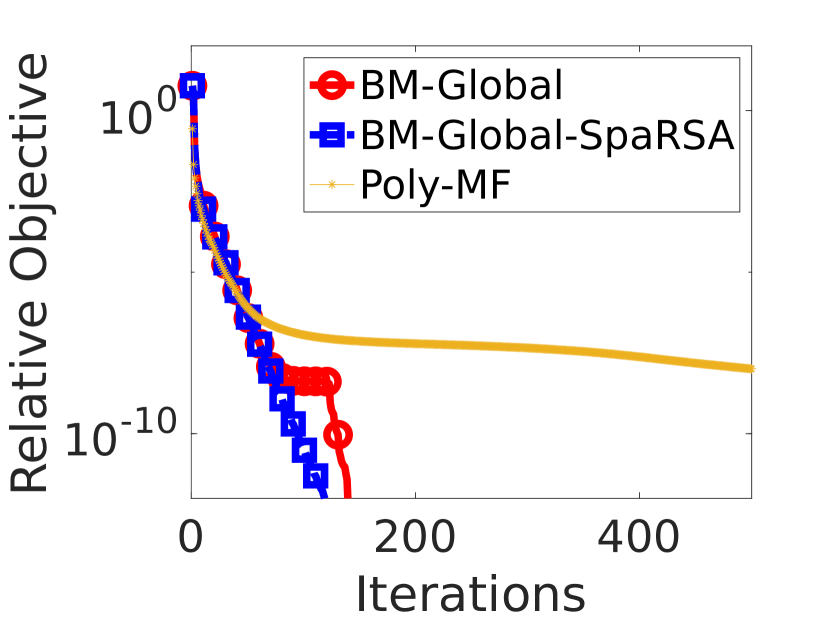
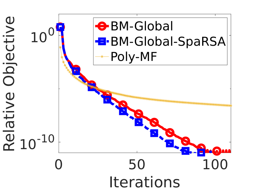
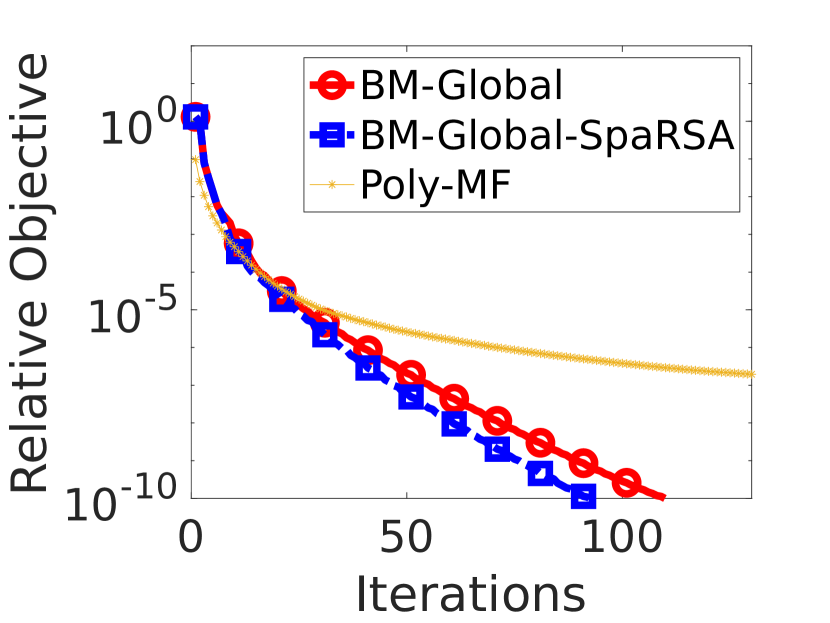
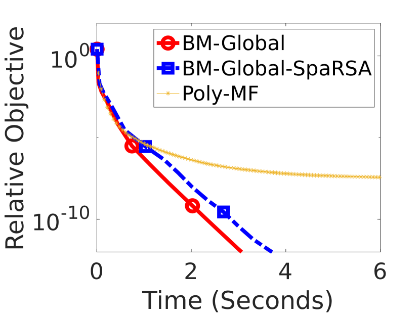
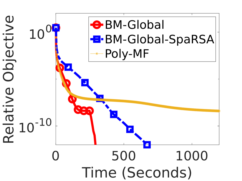
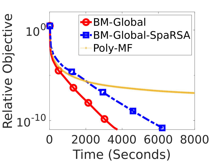
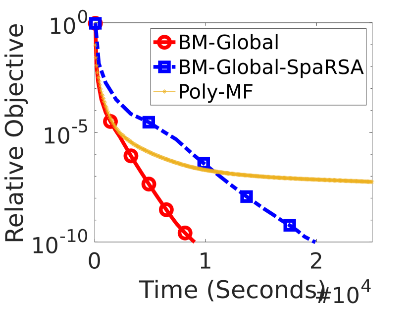
II.4 Parallelism
We also examine the parallelism of our method. In particular, we run our method with cores and check how much time they respectively take to make Eq. 74 no larger than , and compute the speedup as follows.
We can observe from Fig. (V) that except for the small dataset movielens100k, PolyMF-SS always achieves the highest speedup because most of its operations are inherently parallel and computationally heavy, and BM-Global comes the next, while AIS-Impute and Active-ALT barely exhibit any parallelism at all.
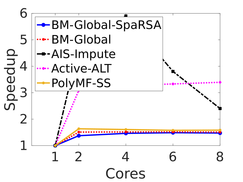
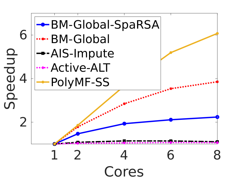
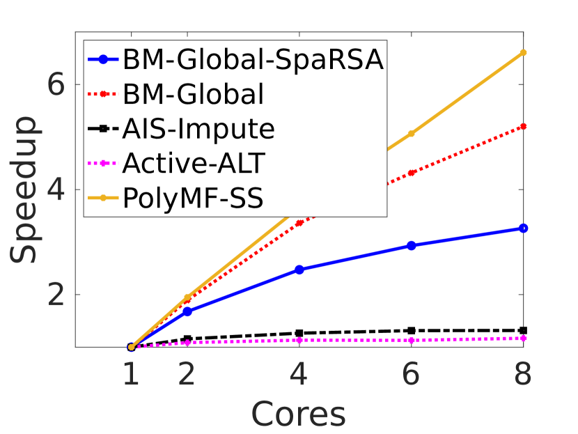
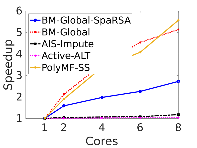
II.5 Numerical results for the APG method
This subsection presents numerical results of the APG method Algorithm 3 on testing problems considered in Section 6.2.
In our experiments, the APG method is executed with and a fixed step size , where is estimated by the eigs subroutine in MATLAB. To perform the projection through Lemma 7, we use the eig subroutine in MATLAB. Our stopping condition for the APG method is
where tol is the tolerance (chosen as in our experiments). Moreover, we set the maximal number of iterations to be and the maximal computational time to be four hours. The computational results for the RKE problems and the molecular conformation problems are presented in Tables (VI) and (VII), respectively. We can observe from the presented results that the APG method usually performs worse than BM-Global and QSDPNAL. Indeed, it returns solutions with a lower accuracy and takes more computational time. Also, the numerical results suggest that the APG method could be sensitive to the sign of the parameter , since it performs much better in the cases of then in the cases of .
| Name | rnk | Time | Iter | |||
|---|---|---|---|---|---|---|
| BrainMRI | 124 | 2e-16 | 1e-03 | 5 | 0.7 | 86 |
| protein | 213 | 3e-15 | 1e-03 | 27 | 6.7 | 285 |
| CoilDelftDiff | 288 | 2e-15 | 1e-03 | 32 | 9.0 | 234 |
| coildelftsame | 288 | 3e-15 | 2e-03 | 32 | 7.7 | 189 |
| CoilYork | 288 | 1e-15 | 1e-03 | 21 | 9.2 | 231 |
| Chickenpieces-5-45 | 446 | 4e-16 | 2e-03 | 28 | 32.6 | 288 |
| newgroups | 600 | 3e-17 | 2e-03 | 84 | 69.7 | 341 |
| flowcytodis | 612 | 8e-16 | 1e-03 | 16 | 84.6 | 353 |
| DelftPedestrians | 689 | 2e-15 | 2e-03 | 70 | 105.0 | 377 |
| WoodyPlants50 | 791 | 8e-16 | 2e-03 | 49 | 185.7 | 478 |
| delftgestures | 1500 | 1e-15 | 1e-02 | 106 | 283.3 | 191 |
| zongker | 2000 | 1e-15 | 4e-03 | 303 | 1236.5 | 451 |
| polydish57 | 4000 | 2e-15 | 1e-02 | 139 | 8530.7 | 357 |
| polydism57 | 4000 | 3e-15 | 1e-02 | 83 | 8023.2 | 337 |
| Name | rnk | RMSD | Time | Iter | |||
|---|---|---|---|---|---|---|---|
| 1PBM | 126 | 4e-16 | 6e-06 | 14 | 7.4 | 30.1 | 5073 |
| 1AU6 | 161 | 2e-16 | 6e-06 | 15 | 6.8 | 55.9 | 5250 |
| 1PTQ | 402 | 2e-15 | 2e-06 | 20 | 10.2 | 727.8 | 10000 |
| 1CTF | 487 | 5e-16 | 2e-06 | 23 | 11.2 | 1250.5 | 10000 |
| 1HOE | 558 | 1e-15 | 2e-06 | 24 | 11.6 | 1831.3 | 10000 |
| 1LFB | 641 | 1e-15 | 2e-06 | 28 | 13.4 | 2379.5 | 10000 |
| 1PHT | 666 | 5e-16 | 2e-06 | 28 | 12.2 | 2598.5 | 10000 |
| 1F39 | 767 | 1e-15 | 2e-06 | 33 | 13.6 | 3432.6 | 10000 |
| 1DCH | 806 | 3e-17 | 2e-06 | 32 | 13.4 | 3776.6 | 10000 |
| 1HQQ | 891 | 1e-15 | 2e-06 | 41 | 15.0 | 4539.2 | 10000 |
| 1POA | 914 | 9e-16 | 2e-06 | 37 | 14.2 | 4844.0 | 10000 |
| 1AX8 | 1003 | 8e-16 | 2e-06 | 40 | 14.3 | 5969.8 | 10000 |
| 1TJO | 1394 | 2e-15 | 2e-06 | 62 | 19.0 | 12512.3 | 10000 |
| 1RGS | 2015 | 6e-16 | 4e-06 | 126 | 20.2 | - | 4952 |
| 1TOA | 2138 | 2e-15 | 5e-06 | 136 | 19.2 | - | 4303 |
| 1KDH | 2846 | 5e-16 | 1e-05 | 254 | 21.9 | - | 1901 |
| 1NFG | 3501 | 3e-15 | 5e-05 | 391 | 21.2 | - | 903 |
| 1BPM | 3672 | 2e-16 | 6e-05 | 436 | 23.8 | - | 788 |
| 1MQQ | 5510 | 7e-16 | 3e-04 | 888 | 26.0 | - | 247 |