greed: An R Package for Model-Based Clustering by Greedy Maximization of the Integrated Classification Likelihood

Etienne Côme, Nicolas Jouvin greed: An R Package for Model-Based Clustering by Greedy Maximization of the Integrated Classification Likelihood greed: Model-Based Clustering with the Integrated Classification Likelihood The greed package implements the general and flexible framework of come2021hierarchical for model-based clustering in the R language. Based on the direct maximization of the exact Integrated Classification Likelihood with respect to the partition, it allows jointly performing clustering and selection of the number of groups. This combinatorial problem is handled through an efficient hybrid genetic algorithm, while a final hierarchical step allows accessing coarser partitions and extract an ordering of the clusters. This methodology is applicable in a wide variety of latent variable models and, hence, can handle various data types as well as heterogeneous data. Classical models for continuous, count, categorical and graph data are implemented, and new models may be incorporated thanks to S4 class abstraction. This paper introduces the package, the design choices that guided its development and illustrates its usage on practical use-cases. R, model-based, clustering, hierarchical, classification likelihood, genetic algorithms R, model-based, clustering, hierarchical, classification likelihood, genetic algorithms Etienne Côme
COSYS - GRETTIA
Université Gustave Eiffel

F-77454 Marne-la-Vallée
Marne La Vallée
E-mail:
Nicolas Jouvin
UMR 518 MIA Paris-Saclay
INRAE, AgroParisTech
Université Paris-Saclay
16 rue claude bernard, 75005 Paris
Paris
E-mail:

1 Introduction

Clustering consists in the unsupervised task of grouping a set of objects into distinct groups or clusters. Unveiling relevant structure in datasets, it holds an important part in modern data analysis, with a wide range of applications involving data of different nature. Grounded on a statistical approach, model-based clustering provides a flexible method capable of handling the variety and complexity of modern data such as continuous, count, graphs or mixed data in a common framework using finite mixtures or stochastic block models (bouveyron2019model). The greed R package, introduced in this paper, builds on this general framework and provides a generic method for clustering various types of data based on the maximization of the Integrated Classification Likelihood (come2021hierarchical). The method is versatile and thanks to the exploration capabilities of an hybrid genetic algorithm, it does not rely on a carefully chosen - and potentially costly and model dependent - initialization procedures. Throughout the paper, we will discuss specific instances of models and give suitable references for related works and packages for each of the considered data type: count, continuous, mixed-type and graph data.

The clustering problem has been the focus of a lot of attention in the last decades, and the R (Rcore) community have been a driving force with the development of many packages taking advantage of the R programming language capacities in handling and visualizing data. These packages can be divided into three main categories:

1. On the one hand, there are packages implementing distance-based clustering, relying on some ad hoc notion of similarity between observations. Working with vector-valued observations, the well-known k-means (macqueen1967some) algorithm is implemented in the stats and ClusterR (ClusterR) packages for Euclidean distances. Refined similarity metrics for k-means such as kernels are available in the kernlab package (kernlab), together with an implementation of the spectral clustering algorithm (ng2002spectral). Other partitional methods working with k-medoids and arbitrary distance functions are implemented in the cluster package (clusterpackage). Finally, the clustMixType (clustMixType) package allows to cluster mixed type data composed of numeric and categorical variables. On the side of graph clustering algorithms, the well-known Louvain algorithm (blondel2008fast) based on modularity maximization is implemented in the igraph (igraph), and the spectral clustering algorithm is also very popular for clustering binary or weighted adjacency matrices.

2. On the other hand, packages implementing model-based clustering fit a probabilistic model to the data. We distinguish between two main strategies for statistical inference:

   1. Frequentist: The first strategy casts clustering as a parameter estimation problem, traditionally dealt with via maximum likelihood, and most of the time solved with the help of some (possibly variational) EM procedure. The clustering comes as a byproduct since a partition can then be obtained via its posterior distribution given the observation and the point estimates. This approach is implemented in various R packages such as Mclust (Mclust) for Gaussian mixture models, mixtools (mixtools) for multinomial mixtures, poLCA (poLCA) for mixture of categorical distributions, and blockmodels (blockmodels) and sbm (sbm) for the simple and bipartite stochastic block models (SBM). The Rmixmod (Rmixmod) package also provides an R interface with the MIXMOD software to fit Gaussian or categorical mixtures for continuous or count data clustering. Somewhat closer to our contribution, the flexmix package (flexmix) also proposes a general framework for fitting mixture models on, possibly heterogeneous, multivariate data using maximum likelihood and an EM procedure. However, it does not cover graph data clustering with SBMs since the latter cannot be cast as simple mixture models and cannot be estimated through regular EM procedures. Their approach is extensible, and new mixture models may be implemented via an S4 class representation of their M-step. While the algorithms strongly differ, our greed package proposes a similar interface, with the possibility to implement new models as S4 classes without impacting the main functions and API.

   2. Bayesian: The second strategy relies on Bayesian inference, seeking to accurately estimate the posterior distribution of the model parameters and cluster memberships, usually via Markov chain Monte Carlo methods (MCMC, robert2013monte). Some of these methods allow inferring the number of clusters through a nonparametric Dirichlet process prior on the group proportions. The main packages implementing Bayesian model-based clustering are rjags (rjags) and rstan (RStan), respectively R interface to the JAGS and STAN softwares, each having dedicated modules for finite mixture modelling. Other packages directly focus on mixture modelling such as Bmix (Bmix), bmixture (bmixture) or IMIFA (IMIFA). Note that, in addition to heavy computations, the two principal difficulties of MCMC inference for clustering are label switching and the resulting multimodality of the posterior.

Beyond the R community, most of the aforementioned methods are implemented in popular Python modules. Without being exhaustive, we mention the scikit-learn module (scikit-learn) implementing standard algorithms for multivariate data clustering in its cluster submodule, and the graph-tool module (graphtool) which implements Bayesian inference for the stochastic block model and its variants.

Our approach lies in between the frequentist and Bayesian approaches, which, while efficient, can be computationally intensive as they require to explore a high-dimensional parameter space, and possibly perform model selection by running the inference procedure on a grid of values for $K$ i.e. the number of clusters. A contrario, we focus on clustering rather than points or posterior estimates of the model parameters, by maximizing an exact version of the Integrated Classification Likelihood (ICL, Biernacki2000) directly with respect to the partition. Originally used as a model selection criterion in frequentist settings, the exact ICL is rooted in the Bayesian framework and consists in the joint distribution of the observations and the partition with all other parameters analytically integrated out by a suitable choice of prior distributions. The genetic algorithm of come2021hierarchical then solves the highly combinatorial problem of maximizing this objective function with respect to the partition, allowing $K$ to be variable, hence performing clustering and model selection altogether while avoiding grid procedures.

In a complementary step, the greed package implements a model-based hierarchical method based on the maximization of a modified ICL criterion. Starting from an initial solution provided by the genetic algorithm, it extracts a hierarchy of nested partitions in an ascendant fashion, by finding the best merge according to this new criterion, similarly to the hclust() function of the stats package. This second step unveils hierarchical structures present in the data, which is useful both for interpretation and visualization (everitt2011cluster, Section 4), while also giving a dendrogram representation of the hierarchy along with a meaningful pseudo-ordering of the clusters.

The paper is organized in the following way. Section 2 briefly introduces the unified statistical framework considered by come2021hierarchical and gives specific instances of models, namely finite mixtures and stochastic block models. Then, Section 3 describes the genetic and hierarchical algorithms along with practical package implementation details. Finally, Section 4 presents an overview of the package’s API and practical guidelines, while LABEL:sec:applications demonstrates its flexibility on practical use-cases, with real-data studies for continuous, categorical, graph and mixed-type data.

2 Model-based clustering

We begin with a brief reminder on model-based approaches to clustering. We will denote as $\bm{\bm{X}}$ the set of observations, which can be a collection of $n$ vectors in $\mathbb{R}^{p}$ in the case of mixture modelling, or an $n\times n$ adjacency matrix in the case of graph clustering. The unobserved partition of $\{1,\ldots,n\}$ will be denoted as $\bm{\bm{Z}}=\{\bm{\bm{z}}_{1},\ldots,\bm{\bm{z}}_{n}\}$ where $\bm{\bm{z}}_{i}$ is a binary vector of size $K$ indicating cluster membership of object $i$.

2.1 Discrete latent variables models

Model-based clustering can be decomposed in a two-stage generative process. First, the partition $\bm{\bm{Z}}$ is drawn from a product of multinomial distributions with parameter $\bm{\bm{\pi}}$, the latter quantifying the a priori probability to belong to each of the $K$ groups. Second, observations are drawn conditionally on the partition, according to some parametric distribution with parameters $\bm{\bm{\theta}}$ depending on the clusters assignments.

Depending on the context, observations may be continuous or discrete vectors in dimension $p$, or edges in a graph. Thus, there are a variety of observational models that can be handled which such an approach. All the models handled by the greed package share the common hypothesis of conditional independence given the full partition $\bm{\bm{Z}}$:

$$p(\bm{\bm{X}},\bm{\bm{Z}}\mid\bm{\bm{\pi}},\bm{\bm{\theta}})=\prod_{\bm{\bm{z}}\in\bm{\bm{Z}}}p(\bm{\bm{z}}\mid\bm{\bm{\pi}})\underset{\text{conditional independence}}{\underbrace{\prod_{\bm{\bm{x}}\in\bm{\bm{X}}}p(\bm{\bm{x}}\mid\bm{\bm{Z}},\bm{\bm{\theta}})}},$$ (1)

Such models are called discrete latent variables models (DLVMs, come2021hierarchical) and popular instances for multivariate data and graph clustering are given in Table 1. For the sake of brevity, we do not detail co-clustering with latent block models (LBM) although it fits the definition of DLVMs and is implemented in greed.

As discussed above, standard frequentist approaches casts clustering as a parameter estimation problem, traditionally dealt with a maximum-likelihood approach solved with the help of some (variational) EM procedure in most cases. The clustering comes as a byproduct since a partition can then be obtained via the posterior distribution of $\bm{\bm{Z}}\mid\bm{\bm{X}},\hat{\bm{\bm{\pi}}},\hat{\bm{\bm{\theta}}}$. This approach is implemented in various R packages such as Mclust (Mclust) for Gaussian mixture models, mixtools (mixtools) for multinomial mixtures, flexmix (flexmix) for general finite mixture models or blockmodels (blockmodels) for the stochastic block model.

Model name	Observation type	Observational model: $\bm{\bm{X}}\mid\bm{\bm{Z}}$
GMM	Multivariate continuous: $\bm{\bm{X}}\in\mathbb{R}^{n\times p}$	$\bm{\bm{x}}_{i}\mid z_{ik}=1,\bm{\bm{\theta}}_{k}\sim\mathcal{N}_{p}(\bm{\bm{x}}_{i}\mid\bm{\bm{m}}_{k},\bm{\bm{S}}_{k})$
MoM	Multivariate discrete: $\bm{\bm{X}}\in\mathbb{N}^{n\times p}$	$\bm{\bm{x}}_{i}\mid z_{ik}=1,\bm{\bm{\theta}}_{k}\sim\mathcal{M}_{p}(\bm{\bm{x}}_{i}\mid\bm{\bm{\theta}}_{k})$
SBM	Graphs: $\bm{\bm{X}}\in\mathbb{R}^{n\times n}$	$x_{ij}\mid z_{ik}z_{jl}=1,\bm{\bm{\theta}}_{kl}\sim p(x_{ij}\mid\bm{\bm{\theta}}_{kl})$

Table 1: Some standard observational models handled by the greed package: Gaussian mixture model (GMM), mixture of multinomial (MoM) and stochastic block models (SBM) for (possibly weighted) graphs. See LABEL:tab:obsmodS4 for a complete list of implemented DLVMs.

2.2 Exact Integrated Classification Likelihood

Having derived an estimate of the model parameters, the choice of the number of clusters $K$ is usually delayed post-inference as a model selection problem (fruhwirth2019handbook, Chapter 7). There exists a large variety of model selection criteria, generally involving a penalized likelihood, such as the Akaike Information Criterion (AIC, akaike1974new) or the Bayesian Information Criterion (BIC, schwarz1978estimating) which are commonly implemented in routine packages. Note that, in this framework, performing clustering and model selection requires to estimate the parameters for a grid of models indexed by $K$, which can be quite cumbersome, even for moderate size problems, as the computational complexity typically grows with $K$.

Hereafter, we focus on the ICL of Biernacki2000, a widely used model selection criterion in the clustering context. Adopting a Bayesian point of view on the model parameters $\bm{\bm{\theta}}$ and $\bm{\bm{\pi}}$, it consists in integrating the latter out hence naturally penalizing for complex models. Introducing a factorized prior $p(\bm{\bm{\theta}},\bm{\bm{\pi}})=p(\bm{\bm{\theta}}\mid\bm{\beta})p(\bm{\bm{\pi}}\mid\bm{\bm{\alpha}})$ with respective hyperparameters $\bm{\beta}$ and $\bm{\bm{\alpha}}$, the $\operatorname{ICL}$ writes as:

$$\operatorname{ICL}(\bm{\bm{Z}};\bm{\bm{\alpha}},\bm{\beta})=\log\int p(\bm{\bm{X}}\mid\bm{\bm{\theta}},\bm{\bm{Z}})p(\bm{\bm{\theta}}\mid\bm{\beta})\mathop{}\!\mathrm{d}\bm{\bm{\theta}}+\log\int p(\bm{\bm{Z}}\mid\bm{\bm{\pi}})p(\bm{\bm{\pi}}\mid\bm{\bm{\alpha}})\mathop{}\!\mathrm{d}\bm{\bm{\pi}}.$$ (2)

Such integrals are typically non-analytic and usually approximated via Laplace method, leading to a penalized likelihood criterion à la BIC.

However, it is possible to derive exact version of the ICL by choosing conjugate priors for the model parameters $p(\bm{\bm{\theta}}\mid\bm{\beta})$ and $p(\bm{\bm{\pi}}\mid\bm{\bm{\alpha}})$:

$$\operatorname{ICL_{\textit{ex}}}(\bm{\bm{Z}};\bm{\bm{\alpha}},\bm{\beta}) =\log p(\bm{\bm{X}}\mid\bm{\bm{Z}},\bm{\beta})+\log p(\bm{\bm{Z}}\mid\bm{\bm{\alpha}}).$$ (3)

The first term of the right-hand side is model-dependent, and must be computed on a case-by-case basis as it depends on the prior on the observational model parameters $\bm{\bm{\theta}}$. However, putting a symmetric Dirichlet prior ${p(\bm{\bm{\pi}})=\operatorname{Dir}(\bm{\bm{\pi}}\mid\bm{\alpha}=(\alpha,\ldots,\alpha))}$ over the group proportions, the second term is universal to any DLVM and is derived thanks to Dirichlet-Multinomial conjugacy:

$$\operatorname{ICL_{\textit{ex}}}(\bm{\bm{Z}};\alpha,\bm{\beta})=\log p(\bm{\bm{X}}\mid\bm{\bm{Z}},\bm{\beta})+\log\left(\dfrac{\Gamma(K\alpha)\prod\limits_{k=1}^{K}\Gamma(\alpha+n_{k})}{\Gamma(\alpha)^{K}\Gamma(n+\alpha\,K)}\right),$$ (4)

where $n_{k}$ is the number of individuals in cluster $k$.

3 Algorithms

3.1 Greedy maximization of the exact ICL

In contrast to inference-based approaches, the greed package bypasses the statistical inference step and focuses on the clustering objective of jointly finding some hard-partitioning $\bm{\bm{Z}}$ as well as its number of clusters $K$. This is done by solving the maximization of $\operatorname{ICL_{\textit{ex}}}$ with respect to both $(\bm{\bm{Z}},K)$:

$$\bm{\bm{Z}}^{(K^{\star})}\in\operatorname*{arg\,max}_{K,\bm{\bm{Z}}}\operatorname{ICL_{\textit{ex}}}(\bm{\bm{Z}},K),$$ (5)

the greed package implements several algorithms tackling this problem. Naturally, due to the highly multimodal and combinatorial nature of this discrete problem, the proposed algorithms are not guaranteed to converge to a global maximum, but rather to efficiently explore the space of solutions to find relevant local optima at a reasonable computational time and cost.

The default algorithm used by the greed package is a hybrid genetic algorithm (GA), introduced in detail in (come2021hierarchical). Standard GAs evolve a population of solutions by selecting some of the most promising ones, crossing them, and possibly mutating them until a specified number of generations or some stopping criterion is reached. Their capacity to efficiently explore huge space of solutions makes them ideal candidate for discrete combinatorial optimization problems such as in Equation 5. Moreover, in order to improve the exploitation capacity of GAs around local optima, one may hybrid them with efficient local search algorithms (see Eiben2003, Chap. 10) such as greedy heuristics based on swaps and merge moves. This is the default approach implemented in the greed package, and we detail its most central features as a GA: solution representation and the recombination, mutation and selection operators.

Solutions as partitions.

Since the $\operatorname{ICL_{\textit{ex}}}$ function is invariant under permutations of the cluster indexes, the integer encoding representation in $\bm{\bm{Z}}$ is redundant for our optimization problem. This fact is also known as the label switching problem and have an important impact on the design of the recombination (crossover) operator for GA. Indeed, simple recombination operators based on crossover points will not consider this particularity and will completely break the structure of the solution (Hruschka2009), leading to slow evolution of the population of solutions. One solution to circumvent this issue is to define the crossover and mutation operators directly over the space of partitions $\{1,\ldots,n\}$ into $K$ clusters with a variable $K$, denoted as $\mathcal{P}=\{\bm{C}_{1},...,\bm{C}_{K}\}$. Such operators will not suffer from the label switching problems and will therefore not break the structures already found. The hybrid GA used in greed is based on such operators.

Combining two partitions: the crossover operator.

The crossover operator, recombining two “parents” solutions into a new “child” one, is based on the cross partition operator. The cross partition of two partitions is simply the partition built by considering all the possible intersections between the elements of the two partitions being crossed. More formally:

$$\mathcal{P}^{1}\times\mathcal{P}^{2}:=\{\mathbf{C}^{1}_{i}\cap\mathbf{C}^{2}_{j}\,,\,\forall i\in\{1,...,|\mathcal{P}^{1}|\},j\in\{1,...,|\mathcal{P}^{2}|\}\}\setminus\emptyset,$$ (6)

with $\mathcal{P}^{1}=\{\mathbf{C}_{1}^{1},...,\mathbf{C}^{1}_{K_{1}}\}$ and $\mathcal{P}^{2}=\{\mathbf{C}_{1}^{2},...,\mathbf{C}^{2}_{K_{2}}\}$ two partitions of $\{1,...,n\}$. This operator produces a new solution which is a refinement of both solutions being crossed, with at most $|\mathcal{P}^{1}|.|\mathcal{P}^{2}|$ clusters. In practice, the two solutions being crossed will agree on some clusters and the number of new clusters after crossover will be smaller. It also defines the coarser clustering which can lead to either $\mathcal{P}^{1}$ or $\mathcal{P}^{2}$ using merge operations, i.e. their first common ancestor in the partition lattice. Thus, in case of under-fitting of both parent partitions, crossing alone may already improve the solution. Finally, while this crossing may create superfluous clusters when done near local maxima of $\operatorname{ICL_{\textit{ex}}}$, the greedy local search based on merges used in the hybrid GA efficiently removes these extra clusters.

Mutation & selection.

The remaining aspects to set up concern the selection procedures and the mutation operators. For the selection process, the hybrid GA algorithm uses a classical rank-based selection policy (see Eiben2003, p. 81-82). In this scheme, at each step, the $V$ solutions selected for building the next generation are selected according to a probability proportional to their rank in terms of $\operatorname{ICL_{\textit{ex}}}$. Eventually, regarding the mutation operator, the hybrid GA algorithm splits a random cluster in two at random. Indeed, while the greedy heuristic, consisting in swaps and merges, can decrease the complexity of the solutions, it is unable to refine a partition. Such a mutation, along with the recombination operator, will help the exploration of candidate solutions with more clusters.

Eventually, note that the first generation of candidates build by the hybrid-GA algorithm are constructed using a simple greedy swap algorithm from totally random starting partitions. Greedy hill-climbing heuristics are therefore used at initialization (swaps) and after each recombination (merges) and mutations (swaps).

Finally, the greed package also comes along with three other optimization algorithms that the user may decide to use for comparison or if suitable:

• A classical genetic algorithm without hybridization with greedy local search.

• A classical greedy hill climbing (swap and merge) algorithm with multiple random starting partitions (see e.g. come2015, for the SBM) .

• A classical greedy hill climbing algorithm (come2015) with one seeded starting point, the seed being produced by a model-dependent heuristic (over-segmented $K$-means for GMM as an example).

3.2 Hierarchical clustering and cluster ordering

Once a solution with a number $K^{*}$ of clusters have been found by one of the previous algorithms, the greed package also provides a hierarchical approach to build a set of $\operatorname{ICL}$ dominant solutions for all the value of $K$ between $K^{*}$ and 1 (see come2021hierarchical, for details). This is achieved in the same Bayesian paradigm with the $\operatorname{ICL_{\textit{ex}}}$ objective, now considering the Dirichlet prior parameter $\alpha$ as a regularization controlling the granularity of the clustering and unlocking access to simpler, coarser, solutions as it decreases towards $0$. The method is based on a log-linear approximation of $\operatorname{ICL_{\textit{ex}}}$ when $\alpha$ is small, which makes it computationally efficient, and produces a hierarchy of nested partitions along with the sequence of the regularization parameters which enabled the fusions $(\bm{\bm{Z}}^{(k)},\,\alpha^{(k)})_{k=K^{\star},\ldots,1}$. Each of these partitions is dominant in terms of $\operatorname{ICL}$ when $\alpha$ is in the value range between $\alpha^{(k-1)}$ and $\alpha^{(k)}$. Such a hierarchical processing allows for the exploration of the clustering at coarser scales, together with an optimal ordering of the clusters which is a powerful tool both for visual representation of the results and their analysis. This final ordering is computed in an optimal fashion in order to minimize the sum of merging costs between adjacent clusters while respecting the order constraints imposed by the merge tree (come2021hierarchical, Section 4). This can be done efficiently thanks to the dynamic programming algorithm of Bar2001. It is particularly useful for the dendrogram representation of the hierarchy and other visualization tools described in LABEL:sec:applications.

3.3 Implementation details

One of the main features of the greed package is its flexibility, as it can handle any observational model, i.e. any DLVM, for which a tractable exact $\operatorname{ICL}$ expression can be derived. The implementation reflects this fact and, while most of the standard DLVMs are implemented, new observational models can seamlessly be integrated without impacting the main functions and API. Each observational model must obey an interface and implements methods that compute the difference of $\operatorname{ICL_{\textit{ex}}}$ induced by an elementary change of a solution (i.e. a swap or a merge) and to compute the observational part of the $\operatorname{ICL_{\textit{ex}}}$ criterion in Equation 3, denoted as $\log p(\bm{\bm{X}}\mid\bm{\bm{Z}},\bm{\beta})$. For the available models, the swap and merge moves are efficiently implemented, only updating the necessary terms rather than computing the whole $\operatorname{ICL_{\textit{ex}}}$ twice and taking the differences. Moreover, whenever possible we took advantage of possible computational speedups, e.g. for Mixture of regressions models we used Woodbury identity to efficiently perform rank-one updates of the inverse of the covariance matrices induced by the swaps.

The remaining part of the code base is generic for all models. On the computational side, the main demanding methods were developed in C++ thanks to the Rcpp package (Eddelbuettel2017) taking advantages of sparse matrix computational efficiency provided by the RcppArmadillo and Matrix packages (Eddelbuettel2014; Bates2019). The greedy swap and merge methods are implemented in C++ and the high-level optimization algorithms GA, hybrid GA, multiple restarts and seeded greedy algorithms in R. Eventually, the future package (Bengtsson2019) was used to enable easy parallelization of the computations in the hybrid GA and multistarts algorithms. Finally, the observational model and the optimization algorithm are defined with S4 classes which we detail in the next section on some concrete use cases.

A note on numerical performances and algorithms complexities.

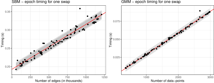
Figure 1: Timings of one swap pass for the SBM (left) and Diagonal-GMM (right) models. For the SBM, the data were simulated using a planted partition model with 4 equiprobable clusters, 4000 nodes, an off-diagonal connection probability of $10^{-3}$ and a diagonal connection probability drawn at random between $0.01$ and $0.3$. This scheme leads to graphs with 250K to 1.25M edges. For the GMM, the datasets were simulated with a 3-component GMM in dimensions $10$. The number of data points was drawn at random between 300 and 3000. In both cases, the swap algorithm was initiated with $K=10$ clusters and 80 datasets were simulated. The timings were done on a Xeon(R) CPU, at 3.50GHz, and without parallelization.

All the optimization algorithms proposed by the greed package rely on combinations of locally optimal swap and merge moves. The time complexity of the latter are model dependent: a whole epoch of swap moves for an SBM (or it’s degree corrected version) is in $\mathcal{O}(M\cdot K^{2})$, with $M$ the number of edges in the graph and $K$ the current number of clusters, whereas it reaches a complexity in $\mathcal{O}(N\cdot K\cdot D)$ for a Diagonal-GMM model. Figure 1 clearly illustrates this relationship on simulated data for both models. The timings are shown for one epoch of a swap, and the linear relationships with the number of edges for SBM and with the number of data-points for GMM clearly appears. The timings are reasonable with respect to the problems sizes.

Regarding the merge moves, the complexities are also model dependent. However, as in standard agglomerative procedures, the necessary statistics only have to be computed once at the beginning. For example, the cost of this operation is in $\mathcal{O}(M)$ for the graphs models and in $\mathcal{O}(N\cdot P)$ for classical mixture, where $P$ is a model dependent constant. Then, the cost of computing the $\operatorname{ICL_{\textit{ex}}}$ variation for one merge is in $\mathcal{O}(P)$, with $P=K$ for SBM like models and $P=d$ for Diagonal-GMM models, for example. Note that it does not depend on $N$ or $M$ anymore. Merge moves are used twice in the algorithm: first in the GA in order to merge redundant clusters after the cross-partition operator in Equation 6, and second in the hierarchical clustering algorithm used to complete the hierarchy after the genetic algorithm has converged. These two use cases do not exhibit the same overall complexity. Indeed, the GA takes advantage of the specific structure yielded by the cross-partition operator to avoid exploring irrelevant pairs of clusters. To do so, merge moves are only considered between pairs of clusters that share a common parent in one of the two parent partitions, see come2021hierarchical for details. Moreover, the hierarchy is not built entirely during the GA greedy merge steps, hence further reducing the computational costs. Thus, in practice, the greedy merge heuristic does not reach its worst-case complexity - which is in $\mathcal{O}(K^{2}\cdot(K+P))$ - during the GA, and it is quite economical compared to the swaps operations costs thanks to the low values of $K$. Concerning the final hierarchical step algorithm, after the GA convergence, the complete hierarchy is built and all possible merges are considered at each step. Therefore, its complexity reaches the bound $\mathcal{O}(K^{2}\cdot(K+P))$, which is still reasonable for low values $K=K^{\star}$ found by the GA.

Naturally, discussing each global algorithm complexity is quite difficult, since they are influenced by many factors such as population size, number of generations before convergence, mutations probabilities, etc. Nevertheless, one may put in perspectives the different use cases of the algorithms: the hybrid-GA and multistarts algorithms are quite comparable in terms of computational time, provided that the population size of the hybrid-GA is equal to the number of starting points of the multistarts algorithm. The former being more efficient than the latter on all the implemented models, it is the default of the package. The seeded algorithm may be advantageous to users that want to quickly explore large datasets, provided that the seeding algorithm is efficient. Indeed, it is less computationally intensive since only one swap epoch is performed, compared to several dozen for multistarts and hybrid-GA.

A notable aspect of the package is its ability to handle graphs with thousands of nodes in a very reasonable amount of time (less than 1 minute) making it competitive with respect to existing frequentist or Bayesian approaches. As an illustration, in the simulation settings of Figure 1, the whole procedure runs in 30.2 seconds on average for a SBM graph with 4000 nodes and more than 400K edges.

Finally, greed is seamlessly adaptable to parallel computing as described in LABEL:subsec:future. This can be easily used to obtain a sensible speedup in performance when datasets become large.

4 Guidelines for Users

This section provides an overview of a basic usage of the package. We also describe the S4 classes and methods facilitating the manipulation and exploration of the results. As a complement to this section and to the usual R package documentation, a complete documentation including model-specific vignettes is available as a pkgdown website at https://comeetie.github.io/greed/.

4.1 The greed function

The package’s main entry point is the greed() function, which performs the clustering and presents a flexible API as illustrated in the block of code below.

R> library("greed") R> sol = greed( + X , # dataset to cluster + K = 20 , # number of initial clusters (optional) + model = Gmm() , # model to use and its prior parameters (optional) + alg = Hybrid() , # algorithm to use and its parameters (optional) + verbose= FALSE ) # verbosity level (optional)

The greed() function only has one mandatory argument, X, which contains a dataset to cluster. All remaining arguments are optional:

• K represents the initial number of clusters and is set to 20 by default. Note that this value is an initial guess, and the available optimization algorithms may return a partition with more or less clusters.

• model is an S4 object inheriting of the abstract class DlvmPrior and containing the observational model used to compute $\operatorname{ICL_{\textit{ex}}}$ along with its (model-specific) hyperparameters. If not provided, greed will try to infer a compatible model with the provided dataset. For example, if X is a symmetric binary sparse dgCmatrix the model will be set to an Sbm() model. Or else, if the provided dataset is a data.frame with only columns of factor type, an Lca() model will then be used. The list of available observational models, their prior parameters and allowed inputs is summarized in LABEL:tab:obsmodS4.

• alg determines the clustering algorithm used by the greed() function. The algorithm is an S4 object inheriting from the abstract Alg class and containing the relevant hyperparameters (e.g. probability of mutation, etc.). By default, the hybrid GA described in Section 3 is used, but other maximization heuristics may be used such as standard greedy hill-climbing with multiple random starts, or a standard GA without greedy local search.

4.2 Analysing the clustering result

The greed() function return an S4 object that inherits from the IclPath S4 class, e.g. a SbmPath object when the model used is an Sbm or a GmmPath object when the model used is a Gmm. Thus, any clustering result shares the same structure and can be analyzed with the same set of S4 methods, independently from the specified model, illustrating the generic aspect of the methodology. These methods are listed in Table 2 along with their description, and LABEL:sec:applications presents several uses in concrete examples.

Method name	Description
clustering(sol)	Returns the estimated partition, integer encoded.
K(sol)	Returns the number of clusters of the partition.
ICL(sol)	Returns the ICL value of the partition.
prior(sol)	Returns the model object used in the call to greed, with eventually the hyper-parameter values that were used during the fit and fixed automatically in a data-driven way.
cut(sol, K)	Cut the dendrogram at specified level K and returns the corresponding IclPath object. Similar to stats::cutree().
coef(sol)	Returns the MAP estimates of the model parameters $\bm{\bm{\theta}}$ conditionally on the estimated partition in a named list.
plot(sol, type="tree")	Returns a ggplot2 object containing the desired plot type, e.g. dendrogram of the hierarchy or any model-dependent representation of the clustering.

Table 2: S4 methods associated to the IclPath class allowing analysing the results sol of the greed() function.

As a quick illustration, we present the results and usage of these methods in the case of graph clustering with SBM (this model will be presented in more details in LABEL:subsec:sbm) using a nested hierarchical community structure in the simulation. The simulations deals with 12 clusters arranged in three levels: 2 big clusters, each composed of three medium clusters, themselves decomposed in two smaller groups. We choose a community structure where nodes inside the same blocks tend to connect more. The connectivity matrix $\bm{\bm{\theta}}$ of the simulation is displayed in Figure 2 and the model in LABEL:eq:sbm.

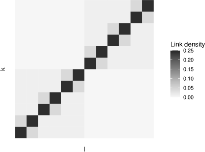
Figure 2: Connectivity matrix of the SBM hierarchical simulation.

R> N <- 800 # Number of node R> K <- 12 # Number of cluster R> pi <- rep(1/K,K) # Clusters proportions R> sbmsim <- rsbm(N,pi,theta) # Simulation R> sol <- greed(sbmsim$x,model=Sbm())\mathrm{\#}ClusteringThealgorithmfoundthetrueclusteringstructure.Inaddition,thedendrogramandtheblockadjacencymatrixof\text{<span class="ltx\_ref ltx\_missing\_label ltx\_font\_italic ltx\_ref\_self">LABEL:fig:example-dendo</span>}highlightthehierarchicalstructureofthedataset.R>tree<-plot(sol,type=\mathrm{"}tree\mathrm{"})R>blocks<-plot(sol,type={}^{\prime }blocks{}^{\prime })R>ggarrange(blocks,tree)\text{Figure 3Figure 3fig.Figurefigs.Figures3Figure 33Blocksrepresentation(}$