iHub, Radboud University Nijmegen, The Netherlandsdario.stein@ru.nl Humming Inc., United States of Americarichard@heyhumming.com \CopyrightDario Stein, Richard Samuelson {CCSXML} <ccs2012> <concept> <concept_id>10003752.10003753.10003757</concept_id> <concept_desc>Theory of computation Probabilistic computation</concept_desc> <concept_significance>500</concept_significance> </concept> <concept> <concept_id>10003752.10010124.10010131.10010133</concept_id> <concept_desc>Theory of computation Denotational semantics</concept_desc> <concept_significance>500</concept_significance> </concept> <concept> <concept_id>10003752.10010124.10010131.10010137</concept_id> <concept_desc>Theory of computation Categorical semantics</concept_desc> <concept_significance>500</concept_significance> </concept> <concept> <concept_id>10002950.10003648</concept_id> <concept_desc>Mathematics of computing Probability and statistics</concept_desc> <concept_significance>500</concept_significance> </concept> </ccs2012> \ccsdesc[500]Theory of computation Probabilistic computation \ccsdesc[500]Theory of computation Categorical semantics \ccsdesc[500]Mathematics of computing Probability and statistics
Acknowledgements.
It has been useful to discuss this work with many people. Particular thanks go to Tobias Fritz, Bart Jacobs, Dusko Pavlovic, Sam Staton and Alexander Terenin.\relatedversiondetails[cite=stein2022decorated]Previous Versionhttps://arxiv.org/abs/2204.14024v1 \EventEditorsPaolo Baldan and Valeria de Paiva \EventNoEds2 \EventLongTitle10th Conference on Algebra and Coalgebra in Computer Science (CALCO 2023) \EventShortTitleCALCO 2023 \EventAcronymCALCO \EventYear2023 \EventDateJune 19–21, 2023 \EventLocationIndiana University Bloomington, IN, USA \EventLogo \SeriesVolume270 \ArticleNo13A Category for unifying Gaussian Probability and Nondeterminism
Abstract
We introduce categories of extended Gaussian maps and Gaussian relations which unify Gaussian probability distributions with relational nondeterminism in the form of linear relations. Both have crucial and well-understood applications in statistics, engineering, and control theory, but combining them in a single formalism is challenging. It enables us to rigorously describe a variety of phenomena like noisy physical laws, Willems’ theory of open systems and uninformative priors in Bayesian statistics. The core idea is to formally admit vector subspaces as generalized uniform probability distribution. Our formalism represents a first bridge between the literature on categorical systems theory (signal-flow diagrams, linear relations, hypergraph categories) and notions of probability theory.
keywords:
systems theory, hypergraph categories, Bayesian inference, category theory, Markov categoriescategory:
\relatedversion1 Introduction
Modelling the behavior of systems under uncertainty is of crucial importance in engineering and computer science. We can distinguish two different kinds of uncertainty:
-
•
Probabilistic uncertainty means we may not know the exact value of some quantity, like a measurement error, but we do know the statistical distribution of such errors. A typical such distribution is the normal (Gaussian) distribution of mean and variance .
-
•
Nondeterministic uncertainty models complete ignorance of a quantity. We know which values the quantity may feasibly assume but have no statistical information beyond that. Nondeterministic uncertainty can be modelled using subsets which identify the feasibles values. In practice, such subsets are often characterized by equational constraints such as natural laws.
Systems may be subject to both probabilistic and nondeterministic constraints, but describing such systems mathematically is more challenging. A classical treatment is Willems’ theory of open stochastic systems [38, 37], where ‘openness’ in his terminology refers to nondeterminism or lack of information. We recall a simple example:
Example 1.1 (Noisy resistor).
For a resistor of resistance , Ohm’s law constrains pairs of voltage and current to lie in the subspace . This is a relational constraint – values must lie in , but we have no further statistical information about which values the system takes. In a realistic system, thermal noise is always present; such a noisy system is better modelled by the equation
| (1) |
where is a Gaussian random variable with some small variance . Willems notices that the variables are not random variables in the usual sense; we have not associated any distribution to them. On the other hand, the quantity is a honest random variable. Furthermore, if we supply a fixed voltage , we can solve for and
| (2) |
becomes a classical (Gaussian) random variable. Willems calls this ‘interconnection’ of systems.
Willems models the ‘openness’ of the stochastic systems by endowing the outcome space with an unusually coarse -algebra to formalize the lack of information. Measurable sets are restricted to the form for Borel. The Gaussian probability measure is then only defined on , which essentially makes it a measure on the quotient space . We purely formally define an extended Gaussian distributions on a space as a pair of a subspace and a Gaussian distribution on . In particular, we can think of any subspace as an extended Gaussian distribution . Operationally, sampling a point means picking it nondeterministically from . Every extended Gaussian distribution can be seen as a formal sum of a Gaussian contribution and a nondeterministic contribution .
In our approach, the noisy resistor is described by a single extended Gaussian distribution where is the subspace for for Ohm’s law, and is Gaussian noise in a direction orthogonal to . The marginals are themselves extended Gaussian distributions: we find that and , that is they are picked nondeterministically from the real line, so in this sense we have no information about them. We also find that follows a classical Gaussian distribution without any nondeterministic contribution. The interconnection (2) is obtained as an instance of probabilistic conditioning . We compare our approach to the one of Willems in Section 5.1.
We now describe a completely different situation where it makes sense to admit subspaces as idealized probability distributions, namely uninformative priors in Bayesian inference:
Example 1.2 (Uninformative Priors).
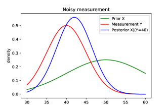
Our prior experience tell us that we expect the mass of some object to be normally distributed with mean and variance . We use a noisy scale to obtain a measurement of . If the scale error has variance of , we can compute our posterior belief over , which turns out to be 111see appendix 6.2 for the calculation . Here, the influence of the prior has corrected the predicted value to lie slightly above the measured value, and have smaller overall variance (see Figure 1).
If we had no prior information at all about , the posterior should simply reflect the measurement uncertainty . We can model this by putting a larger and larger variance on . However, the limit of distributions for does not exist in any measure-theoretic sense, because it would approach the zero measure on every measurable set. There exists no uniform probability distribution over the real line. In practice, one can sometimes pretend (using the method of improper priors, e.g. [19, 22]) that is sampled from the Lebesgue measure (with constant density ). This measure fails to be normalized, however the resulting density calculations may yield the correct probability measures.
Our theory of extended Gaussians avoids unnormalized measures altogether: The nondeterministic distribution is used as the uninformative prior on , which gives the desired results, and can be seen as the limit of for in an appropriate sense.
1.1 Contribution
The paper is devoted to making our manipulations of subspaces as generalized probability distributions rigorous. We introduce a class of mathematical objects called extended Gaussian distributions and show that such distributions can be manipulated (combined, pushed forward, marginalized) as if they were ordinary probability distributions. Importantly, extended Gaussians remain closed under taking conditional distributions, which means we can use them in applications such as statistical learning and Kalman filtering. The subspace , seen as a uniform distribution, formalizes the role of an improper prior.
Describing distributions on a space is only the first step. In order to build up systems in a compositional way, we need to understand transformations between spaces . Category theory is a widely used language to study the composition of different kinds of systems. We identify two relevant flavors in the literature
-
•
categorical and diagrammatic methods for engineering and control theory, such as graphical linear algebra (e.g. [28]), cartesian bicategories (e.g. [6]) and signal-flow diagrams ([4, 3, 5, 2, 1]). A central notion is that of a hypergraph category [13], and prototypical models are the categories of linear maps or linear relations. Willems’ system theory has been explored in these terms [12], but probability is absent from these developments.
- •
Despite these developments, it has been challenging to combine probability and nondeterminism into a single model – mathematical obstructions to achieving this are described in [39, 21]. Our work is a first successful step in combining these bodies of literature: We define a category of extended Gaussian maps which can seen both as extending linear relations with probability, or extending Gaussian probability with nondeterminism (or improper priors). Gaussian probability is a very expressive fragment of probability with a variety of useful applications (Gaussian processes, Kalman filters, Bayesian Linear Regression).
Our definition of the Markov category uses a special case of the widely studied construction of decorated cospans [9, 11, 14, 12]. We recall that has conditionals, which is the categorical formulation of conditional probability used to formalize inference problems like Example 1.2.
We then define a hypergraph category of Gaussian relations, which allows arbitrary decorated cospans to allow the possibility of failure and explicit conditioning in the categorical structure. Hypergraph categories are highly symmetrical categories with an appealing duality theory. To our knowledge, probabilistic models of hypergraph categories are novel. The self-duality of hypergraph categories is reflected in the duality between covariance and precision forms, which takes a particularly canonical form for extended Gaussians. We elaborate this in Section 5.2.
The following table summarizes the relationships between our constructions
| (adding Gaussian noise) | ||
|---|---|---|
| linear maps | Gaussian maps | |
| (adding nondeterminism) | total linear relations | extended Gaussian maps |
| (adding failure) | linear relations | Gaussian Relations |
1.2 Outline
We assume basic familiarity of the reader with linear algebra, (monoidal) categories and string diagrams; an overview can be found in the appendix Section 6. All categories considered will be symmetric monoidal and have a copy-delete structure. All vector spaces are assumed finite dimensional.
We begin Section 2 with a recap of Gaussian probability and continue to define extended Gaussian distributions as Gaussian distributions on quotient spaces. We extend this definition to a notion of extended Gaussian map in Section 3 and establish the structure of a Markov category. We give the construction both in elementary terms and using the formalism of decorated cospans in Section 3.2.
In Section 4, we define a hypergraph category of Gaussian relations, which extends extended Gaussian maps with the possibility of failure and conditioning. This makes use of the discussion of conditionals in Section 4.1.
The idea of extended Gaussian distributions has appeared in several places independently, for different motivations. We conclude the paper with an extended ‘Related Works’ Section 5, which compares these approaches in detail, and gives perspective in terms of measure theory, topology, and program semantics.
2 Extended Gaussian Distributions
We begin with a short review of Gaussian probability; we assume basic concepts of linear algebra but have summarize the terminology in the appendix (Section 6.3). For a more detailed introduction to Gaussian probability see e.g. [35, 24].
The normal distribution or Gaussian distribution of mean and variance is defined by having the density function
with respect to the Lebesgue measure. This is generalized to multivariate normal distributions as follows: Every Gaussian distribution on can be written uniquely as where is its mean and is a symmetric positive-semidefinite matrix called its covariance matrix. Note that a vanishing covariance matrix is explicitly allowed; in that case the Gaussian reduces to a point-mass . We will sometimes abbreviate the point-mass by if the context is clear.
We write for the set of all Gaussian distributions on . The support of is the affine subspace where is the column space (image) of . Gaussian distributions transform as follows under linear maps: If is a matrix, then the pushforward distribution is given by
| (3) |
Product distributions are formed as follows
| (4) |
We write addition between distributions to indicate the distribution of the sum of two independent variables (convolution). For example, if are independent, then because variance is additive for independent variables. We have
which can be confirmed by first forming the product distribution (4) and pushing forward under the addition map (3). The set forms a commutative monoid with convolution and neutral element .
We now wish to a combine Gaussian distributions on with uninformative (nondeterministic) distributions along a vector subspace .
Definition 2.1.
An extended Gaussian distribution on is a pair of a subspace and a Gaussian distribution on the quotient . Following [38], we call the space the (nondeterministic) fibre of the extended Gaussian. We write for the set of all extended Gaussian distributions on .
There are several equivalent ways to formalize the notion of a Gaussian distribution over this quotient space.
-
1.
We identify the quotient space with a complementary subspace of , and give a Gaussian distribution on that space. This has the advantage of only involving Euclidean spaces, and we can use matrices to represent linear maps.
-
2.
We develop a coordinate-free definition of Gaussian distributions on arbitrary vector spaces so we can then interpret the construction directly. This will be useful for the duality results in Section 5.2.
-
3.
Willems keeps the spaces but equips them with restricted -algebras. This corresponds to a quotient on the level of measurable spaces. We discard this perspective for now but will return to it in Section 5.1.
For now, it doesn’t matter which formalization we choose. We will build intuitions with some examples:
-
1.
Every Gaussian distribution becomes an extended Gaussian distribution with ; that is the nondeterministic contribution vanishes (is constantly zero).
-
2.
Every subspace becomes an extended Gaussian distribution with ; that is the probabilistic contribution vanishes. By slight abuse of notation, we will simply write or for the embedding of subspaces or distributions into extended Gaussian distributions.
-
3.
If the nondeterministic fibre is the whole space, then . Hence, the only extended Gaussian with fibre is the subspace itself. This distribution expresses total ignorance.
-
4.
We can easily classify all extended Gaussian distributions on . The fibre must be either or , so we have .
-
5.
The possible pairs satisfying Ohm’s law are given by the subspace . For noisy Ohm’s law, we let and notice that the random vector is orthogonal to . Its covariance matrix is
and thus the distribution of the noisy law is given by .
We may think of the extended distribution as being composed of nondeterminstic noise along the space , and Gaussian noise . It is evocative to write the extended Gaussian distribution as a formal sum of distribution and a subspace. The distribution is not unique because the nondeterministic noise absorbs components of that are parallel to . This is analogous to how we use notation like for elements of quotient groups (cosets). This notation is formally justified by the formula for addition of extended Gaussians, as discussed next.
2.1 Transformations of Extended Gaussians
Extended Gaussian distributions support the same basic transformations as ordinary Gaussians. If is a matrix, we push forward the Gaussian and nondeterministic contribution separately,
where denotes the image subspace. Tensor and sum are similarly component-wise
Well-definedness is a corollary of the next section, because those operations are special cases of the categorical structure of .
Example 2.2.
The subspace absorbs all additive contributions, e.g.
3 A Category of Extended Gaussian maps
After defining extended Gaussians on Euclidean spaces , the next challenge is to develop a notion of extended Gaussian map between spaces. We wish to define a category such that we recover extended Gaussian distributions as maps out of the unit space , i.e. . The operations of pushforward, product and sum of distributions will be simple instances of categorical and monoidal composition in the category . For purely Gaussian probability, the appropriate definition of a map is a linear function together with Gaussian noise, informally written . We begin by analyzing this construction before generalizing it to the extended Gaussian case.
3.1 Decorated Linear Maps and the Category
We write for the category of finite dimensional vector spaces. The category [15] is defined as follows: Objects are vector spaces , and morphisms are pairs of a linear map and a Gaussian distribution . The identity is given by and composition is given by pushing forward and addition of the noise, .
It is straightforward to generalize the pattern of this construction: The set of distributions is a commutative monoid and the assignment becomes a lax monoidal functor from vector spaces to commutative monoids. By understanding a commutative monoid as a one-object category, the functor is an indexed category, and the category is the monoidal op-Grothendieck construction associated to this functor [26].
We do not use any special properties of Gaussian distributions, other than that they can be added and pushed forward. In other words, can think of the distribution as a purely abstract decoration on the codomain of the linear map . Any functor can be used to supply such a decoration, because it it automatically inherits a lax monoidal structure (see below). In concrete terms, the op-Grothendieck construction can be described as decorated linear maps:
Definition 3.1.
Let be a functor. The category of -decorated linear maps is defined as follows
-
1.
Objects are vector spaces
-
2.
Morphisms are pairs where is a linear map and
-
3.
Composition is defined as follows: for , , , let
Note that addition takes place in the commutative monoid .
There is a faithful inclusion sending to . We argue that has the structure of a symmetric monoidal category with the tensor on objects. For this, we first observe that is automatically lax monoidal: For , let where are the biproduct inclusions. We can now define the tensor of decorated map as . The monoidal category is in general not cartesian; it does however inherit copy and delete maps from . The category is a Markov category if and only if deleting is natural, i.e. , where denotes the terminal vector space/commutative monoid.
Example 3.2.
The following categories are instances of decorated linear maps:
-
1.
For , is equivalent to .
-
2.
For , is equivalent to the category of affine-linear maps. A map consists of a pair with linear and .
-
3.
For , is (by construction) the category
3.2 Decorated Cospans and Linear Relations
Like for , we wish to define an extended Gaussian map as a linear map with extended Gaussian noise. The naive approach of considering linear maps decorated by is not fruitful, because the quotient by the nondeterministic fibre is not properly taken into account: For example, for any two linear maps , the decorated maps and should be considered equal (Example 2.2). We can remedy this by considering maps into the quotient . This kind of behavior is precisely captured by (total) linear relations.
Lemma 3.3 (Section 6.3).
To give a total linear relation is to give a subspace and a linear map .
Definition 3.4.
An extended Gaussian map is a tuple where is a subspace, and .
In order to describe composition of such maps, it is convenient to use the formalism of decorated cospans, which we recall now:
A cospan in a category with finite colimits is a diagram of the form . We will identify two cospans if there exists an isomorphism commuting with the legs. Equivalence classes of cospans can be seen as morphisms between and in a category , where composition is given by pushout
| (5) |
The following classes of cospans deserve special attention:
-
1.
a cospan whose right leg is an isomorphism is the same thing as a map
-
2.
a relation is a span which is jointly monic. Dually, a co-relation is a cospan which is jointly epic [11].
-
3.
a partial map is a span whose left leg is monic [8]. Dually we define a copartial map to be a cospan whose right leg is epic.
Just as partial maps are maps out of subobjects, copartial maps are maps into quotients. It is worth noting that while the pushout of copartial maps is again a copartial map, co-relations are not closed under pushout. Instead, the an image factorization has to be used to compose them [11]. Lemma 3.3 can be rephrased as follows:
Proposition 3.5.
To give a copartial map in is to give a total linear relation . The relation is obtained as .
We now use the abstract theory of decorated cospans [9, 10, 14] to add Gaussian probability to the cospans:
Definition 3.6 ([9]).
Given a lax monoidal functor , an -decorated cospan is a cospan together with a decoration . Given composable cospans like in (5), the decoration of the composite is computed by the canonical morphism . The category of -decorated cospans is written
The category is a special case of the decorated cospan construction, for cospans whose right leg is an identity. We can now define:
Definition 3.7.
The category of extended Gaussian maps is defined as the category of copartial maps in , decorated by the functor .
Categories of decorated cospans are hypergraph categories [9, § 2] their monoidal structure is given by the coproduct . As the subcategory of decorated copartial maps, extended Gaussians do inherit the symmetric monoidal and copy-delete structure, but are not a hypergraph category. To obtain a useful hypergraph category of Gaussian probability, we must study conditioning.
4 A Hypergraph Category of Gaussian Relations
A hypergraph category extends the structure of a copy-delete category in two important ways
-
1.
there is a multiplication on every object, which we think of as a comparison operation. It succeeds if both inputs are equal (and return the input), and fails otherwise. In linear relations, comparison is the relation . Multiplication is dual to copying. In a probabilistic setting, we propose to think of the comparison as conditioning on equality. The ‘cap’ is denoted as [25, 33].
-
2.
there is a unit on every object, dual to deletion. The unit is neutral with respect to the multiplication, i.e. conditioning on the unit has no effect. This suggests we should think of the unit as a uniform distribution, or an improper prior. Both in linear relations and extended Gaussians, the unit is the subspace .
We arrive at the following synthetic dictionary for probabilistic inference and constraints in hypergraph categories:
For example, the noisy measurement example Example 1.2 can be expressed in the following convenient way using hypergraph structure
We begin by recalling how conditioning works in the category , and prove that extended Gaussians remain closed under conditioning. We then define a hypergraph category of Gaussian relations in which conditioning is internalized using a comparison operation.
4.1 Conditioning
Gaussian distributions are self-conjugate; that is conditional distributions of Gaussians are themselves Gaussian. More precisely, given a joint distribution , the map which sends is a Gaussian map . This is captured using the following categorical definition:
Definition 4.1 ([15, Definition 11.5]).
A conditional for a morphism in a Markov category is a morphism which lets us reconstruct from its -marginal as . In string diagrams, it satisfies
The category has all conditionals. By picking a convenient complement to the fibre , we can reduce the problem of conditioning in to conditioning in .
Theorem 4.2.
has conditionals.
Proof 4.3.
In the appendix (Section 6.5).
4.2 Gaussian Relations
One difficulty of conditioning is that it introduces the possibility of failure. For example, the condition is infeasible. In general, given a joint distribution , we can only condition if lies in the support of the marginal . The dependence on supports is carefully analyzed in the ‘Cond’ construction of [34].
We define a hypergraph category of Gaussian relations as follows
That is, a Gaussian relation is either a joint extended Gaussian distribution, or a special failure symbol which represents infeasibility. Failure is strict in all categorical operations, i.e. composing or tensoring anything with failure is again failure.
Most of the categorical structure of is easy to define.
-
1.
any morphism can be embedded into as its name given by
-
2.
the identity is the diagonal relation
-
3.
copying and comparison are the both given by the relation
Composition of Gaussian relations requires conditioning: Given and , we compose them as follows: If any of them is , return . Otherwise form the tensor , and condition the two copies of to be equal. If that condition is infeasible, return .
4.3 Decorated cospans as generalized statistical models
We can get a clearer view of composition by using decorated cospans. Recall that decorated copartial functions corresponded to extended Gaussian maps . If we allow arbitrary cospans, we know that the category is a hypergraph category by construction. We now explain how to view such a cospan as a kind of generalized statistical model, whose ‘solution’ is a Gaussian relation.
Theorem 4.4.
We have a functor of hypergraph categories
which sends the decorated cospan with decoration to the Gaussian relation described by the solution to the following inference problem: Initialize and with an uninformative prior. Then condition , and return the posterior distribution in , or if the condition was infeasible.
Decorated cospans thus have an interpretation as a generalized kind of statistical model, and Gaussian relations can be understood as equivalence classes of such cospans which have the same solution. This approach is systematically explored with the Cond construction of [34], and indeed we can see as a concrete representation of .
5 Related Work and Applications
5.1 Open Linear Systems and -algebras
Recall that a probability space is a tuple of a set , a -algebra and a probability measure . A random variable is a function which is -measurable, where denotes the Borel -algebra.
Willems defines an -dimensional linear stochastic system to be a probability space of the form for which there exists a ‘fibre’ subspace such that the -algebra is given by the Borel subsets of in the following sense: Pick any complementary subspace with . Then, the events are precisely Borel cylinders parallel to , i.e. of the form for . As an aside, we might wonder in which sense the the algebra is a quotient construction. The measurable projection is not an isomorphism of measurable spaces; after all, the underlying function is not invertible. It is however an isomorphism in the category of probability kernels, namely the inclusion is an inverse when considered as a stochastic map. This is because the Dirac measures and are equal on . This phenomenon of ‘weak quotients’ is nicely explained in [27, Appendix A].
A linear system is called Gaussian if the measure on is a normal distribution. We notice that this agrees precisely with our definition of an extended Gaussian distribution on with fibre . A linear system is classical only if , in the sense that only in this case the measure is defined on the whole algebra . In the case , the -algebra becomes and we cannot answer any nontrivial questions about the system (Example 2.2).
Willems gives explicit formulas for combining Gaussian linear systems (‘tearing, zooming and linking’) [38]. These operations have been treated in categorical form in [12] but not for probabilistic systems. One fundamental operation in Willems’ calculus is the interconnection of systems: Two probability systems on the same state space are called complementary if for all and , we have
That is, the product of probabilities depends only on the intersection . The two probability measures can now be joined together on the larger -algebra by defining . This is what happens in Example 1.1 when connecting a noisy resistor to a voltage source: The underspecified -algebras gets enlarged and nondeterministic relationships become become probabilistic ones. It seems to us that interconnection is a special case of the composition of Gaussian relations.
It is furthermore interesting that Willems uses the term open for probability systems with an underspecified -algebra on , while in category theory, we think of open systems as morphisms . A remarkable feature is that the -algebra, which in measure-theoretic probability is considered a property of the objects in question (i.e. measurable spaces), is here part of the morphisms. The cospan perspective unifies this, for in a cospan , we can equip with the -algebra generated by the quotient map .
5.2 Variance-Precision Duality
We recall the coordinate-free description of Gaussian probability and use it to show that extended Gaussians are highly symmetric objects, which enjoy an improved duality theory over ordinary Gaussians (reflecting the hypergraph structure of Gaussian relations). This also points towards future research to understand as a topological completion of ordinary Gaussians. Work in this direction is the variance-information manifold of [23]. For simplicity, we will consider only Gaussians of mean zero.
If the covariance matrix is invertible, then its inverse is known as precision or information matrix. Precision is dual to covariance, in the sense that while covariance is additive for convolution , precision is additive for conditioning.
The latter equation is reminiscent of logdensities, which add when conditioning. Indeed, the precision matrix appears in the density function of the multivariate Gaussian distribution .
If we allow singular covariance matrices , we still have well-defined Gaussian distributions albeit with non-full support; however the information matrix ceases to exist (and the distribution no longer has a density with respect to the -dimensional Lebesgue measure). Not only does this break the duality, but we are left to wonder which kind of distribution corresponds to singular precision matrices: The answer is extended Gaussian distributions with nonvanishing fibre.
In a coordinate-free way, the covariance of a distribution is the bilinear form on the dual space given by . This form is symmetric and positive semidefinite. The precision form is instead of type . The duality between the two forms can be stated as follows:
Theorem 5.1.
The following data are equivalent for every f.d.-vector space
-
1.
pairs of a subspace and a bilinear form
-
2.
pairs of a subspace and a bilinear form
At the core of this duality lies the notion of the annihilator of a subspace, here denoted . In brief, the correspondences are as follows
| precision | ||
|---|---|---|
| covariance |
We give a proof of the duality in the appendix (Section 6.3).
5.3 Statistical Learning and Probabilistic Programming
It is unsurprising that notions equivalent to extended Gaussians have appeared in the statistics (e.g. in [22]). A novel perspective on statistical inference which more closely matches the categorical semantics is probabilistic programming, a powerful and flexible paradigm which has gained traction in recent years (e.g. [36, 29, 20]). In [34], we argued that the exact conditioning operation (conditioning on equality) described in Section 4.2 is a fundamental primitive in such programs, and enjoys good logical properties. We presented a programming language for Gaussian probability featuring a first-class exact conditioning operator , with Python/F# implementations available under [30]. For example, the noisy measurement example expressed as a probabilistic program reads
This language uses Gaussian distributions only, but it can effortlessly be extended to use extended Gaussian distributions, which are likewise closed under conditioning (Theorem 4.2).
The behavior of the conditioning operator can be quite subtle, and it is difficult to decide when two programs are observationally equivalent. The denotational semantics defined in [34] on the basis of the category is fully abstract, but it is still lacking a concrete description of when two different programs fragments have the same behavior in all contexts. This is remedied by passing to the concrete description of . In terms of Section 4.3, a program denotes a decorated cospan over , and contextual equivalence is precisely the equivalence relation Theorem 4.4.
The correspondence between probabilistic programs and categorical models of probability (with conditioning) is elaborated in detail in [31].
References
- [1] Baez, J. C., Coya, B., and Rebro, F. Props in network theory, 2018.
- [2] Baez, J. C., and Erbele, J. Categories in control. Theory Appl. Categ. 30 (2015), 836–881.
- [3] Bonchi, F., Sobociński, P., and Zanasi, F. A categorical semantics of signal flow graphs. In CONCUR 2014–Concurrency Theory: 25th International Conference, CONCUR 2014, Rome, Italy, September 2-5, 2014. Proceedings 25 (2014), Springer, pp. 435–450.
- [4] Bonchi, F., Sobocinski, P., and Zanasi, F. The calculus of signal flow diagrams I: linear relations on streams. Inform. Comput. 252 (2017).
- [5] Bonchi, F., Sobociński, P., and Zanasi, F. Interacting Hopf algebras. Journal of Pure and Applied Algebra 221, 1 (2017), 144–184.
- [6] Carboni, A., and Walters, R. Cartesian bicategories i. Journal of Pure and Applied Algebra 49, 1 (1987), 11–32.
- [7] Cho, K., and Jacobs, B. Disintegration and Bayesian inversion via string diagrams. Mathematical Structures in Computer Science 29 (2019), 938 – 971.
- [8] Cockett, J. R. B., and Lack, S. Restriction categories i: categories of partial maps. Theoretical computer science 270, 1-2 (2002), 223–259.
- [9] Fong, B. Decorated cospans. arXiv preprint arXiv:1502.00872 (2015).
- [10] Fong, B. The Algebra of Open and Interconnected Systems. PhD thesis, University of Oxford, 09 2016.
- [11] Fong, B. Decorated corelations, 2017.
- [12] Fong, B., Sobociński, P., and Rapisarda, P. A categorical approach to open and interconnected dynamical systems. In Proceedings of the 31st annual ACM/IEEE symposium on Logic in Computer Science (2016), pp. 495–504.
- [13] Fong, B., and Spivak, D. I. Hypergraph categories. ArXiv abs/1806.08304 (2019).
- [14] Fong, B., and Spivak, D. I. An invitation to applied category theory: seven sketches in compositionality. Cambridge University Press, 2019.
- [15] Fritz, T. A synthetic approach to Markov kernels, conditional independence and theorems on sufficient statistics. Adv. Math. 370 (2020).
- [16] Fritz, T., Gonda, T., and Perrone, P. De Finetti’s theorem in categorical probability, 2021.
- [17] Fritz, T., and Perrone, P. A probability monad as the colimit of spaces of finite samples. arXiv: Probability (2017).
- [18] Fritz, T., and Rischel, E. F. Infinite products and zero-one laws in categorical probability. Compositionality 2 (Aug. 2020).
- [19] Gelman, A., Carlin, J. B., Stern, H. S., and Rubin, D. B. Bayesian Data Analysis, 2nd ed. ed. Chapman and Hall/CRC, 2004.
- [20] Goodman, N. D., Tenenbaum, J. B., and Contributors, T. P. Probabilistic Models of Cognition. http://probmods.org, 2016. Accessed: 2021-3-26.
- [21] Goy, A., and Petrişan, D. Combining probabilistic and non-deterministic choice via weak distributive laws. In Proceedings of the 35th Annual ACM/IEEE Symposium on Logic in Computer Science (New York, NY, USA, 2020), LICS ’20, Association for Computing Machinery.
- [22] Hedegaard, J. N. Gaussian random fields – infinite, improper and intrinsic. Master’s thesis, Aalborg University, 2019.
- [23] JAMES, A. The variance information manifold and the functions on it. In Multivariate Analysis–III. Academic Press, 1973, pp. 157–169.
- [24] Lauritzen, S., and Jensen, F. Stable local computation with conditional Gaussian distributions. Statistics and Computing 11 (11 1999).
- [25] Lavore, E. D., and Román, M. Evidential decision theory via partial markov categories, 2023.
- [26] Moeller, J., and Vasilakopoulou, C. Monoidal Grothendieck construction. arXiv preprint arXiv:1809.00727 (2018).
- [27] MOSS, S., and PERRONE, P. A category-theoretic proof of the ergodic decomposition theorem. Ergodic Theory and Dynamical Systems (2023), 1–27.
- [28] Paixão, J., Rufino, L., and Sobociński, P. High-level axioms for graphical linear algebra. Science of Computer Programming 218 (2022), 102791.
- [29] Staton, S. Commutative semantics for probabilistic programming. In Programming Languages and Systems (Berlin, Heidelberg, 2017), H. Yang, Ed., Springer Berlin Heidelberg, pp. 855–879.
- [30] Stein, D. GaussianInfer. https://github.com/damast93/GaussianInfer, 2021.
- [31] Stein, D. Structural Foundations for Probabilistic Programming Languages. PhD thesis, University of Oxford, 2021.
- [32] Stein, D. Decorated linear relations: Extending gaussian probability with uninformative priors, 2022.
- [33] Stein, D., and Staton, S. Compositional semantics for probabilistic programs with exact conditioning (long version). In Proceedings of Thirty-Sixth Annual ACM/IEEE Conference on Logic in Computer Science (LICS 2021) (2021).
- [34] Stein, D., and Staton, S. Compositional semantics for probabilistic programs with exact conditioning (long version), 2021.
- [35] Terenin, A. Gaussian Processes and Statistical Decision-making in Non-Euclidean spaces. PhD thesis, Imperial College London, 2022.
- [36] van de Meent, J.-W., Paige, B., Yang, H., and Wood, F. An introduction to probabilistic programming, 2018.
- [37] Willems, J. C. Constrained probability. In 2012 IEEE International Symposium on Information Theory Proceedings (2012), pp. 1049–1053.
- [38] Willems, J. C. Open stochastic systems. IEEE Transactions on Automatic Control 58, 2 (2013), 406–421.
- [39] Zwart, M., and Marsden, D. No-go theorems for distributive laws. In Proceedings of the 34th Annual ACM/IEEE Symposium on Logic in Computer Science (2019), LICS ’19, IEEE Press.
6 Appendix
6.1 Glossary: Category Theory
We assume basic familiarity of the reader with monoidal category theory and string diagrams. All relevant categories in this article are symmetric monoidal.
A copy-delete category [7] (or gs-monoidal category) is a symmetric monoidal category where every object is coherently equipped with the structure of a commutative comonoid, which is used to model copying () and discarding () of information. In string diagrams, the comonoid axioms are rendered as
Neither deleting nor copying are assumed to be natural in a copy-delete category. A Markov category is a copy-delete category where deleting is natural, or equivalently, the monoidal unit is terminal. Markov categories typically model probabilistic or nondeterministic computation without possibility of failure, such as stochastic matrices, or total (linear) relations.
Copy-delete categories can model unnormalized probabilistic computation, or the potential of failure. The categories of partial functions or (linear) relations are typical examples of copy-delete categories that are not Markov categories.
A hypergraph category [13] is a symmetric monoidal category with a particularly powerful self-duality: Every object is equipped with a special commutative Frobenius algebra structure.
6.2 Noisy measurement example
Example 6.1.
We elaborate the noisy measurement example from the introduction. Formally, we introduce random variables
The vector is multivariate Gaussian with mean and covariance matrix
The conditional distribution is .
Proof 6.2.
The random vector has joint density function
The conditional density of given has the form
By expanding and ‘completing the square’, it is easy to check that
is again a Gaussian density, from which we read off and .
6.3 Glossary: Linear Algebra
All vector spaces in this paper are assumed finite dimensional. For vector subspaces , their Minkowski sum is the subspace . If furthermore , we call their sum a direct sum and write . A complement of is a subspace such that . An affine subspace is a subset of the form for some and a (unique) vector subspace . The space is called a coset of and the cosets of organize into the quotient vector space .
An affine-linear map between vector spaces is a map of the form for some linear function and . Vector spaces and affine-linear maps form a category .
A linear relation is a relation which is also a vector subspace of . We write . A relation is called total if for all .
Linear relations and total linear relations are closed under the usual composition of relations. We denote by and the categories whose objects are vector spaces, and morphisms are linear relations and total linear relations respectively. is a hypergraph category, while is a Markov category.
The following lemma is crucial for relating linear relations and cospans: Every left-total linear relation can be written as a ‘linear map with nondeterministic noise’ .
Proposition 6.3.
Let be a left-total linear relation. Then
-
1.
is a vector subspace of
-
2.
is a coset of for every
-
3.
the assignment is a well-defined linear map
-
4.
every linear map is of that form for a unique left-total linear relation
Proof 6.4.
For 1, consider (by assumption nonempty), then by linearity of
so is a vector subspace. For 2, we can find some and wish to show that . Indeed if then so , hence . Conversely for all we have so . This completes the proof that is a coset. For 3, the previous point shows that the map is a well-defined map . It remains to show it is linear. That is, if and then . This follows immediately from the linearity of . For the last point 4, given a linear map we construct the relation
which is left-total because . To see that is linear, let meaning and for representatives of . Linearity of means that is a representative of . Thus
6.4 Annihilators
For subspaces and , the subspaces are defined as
| (6) |
Proposition 6.5.
-
1.
Taking annihilators is order-reversing and involutive
-
2.
If , then and we have a canonical isomorphism
(7) and similarly for , we have
(8) -
3.
We have
If and , then
If , we have a canonical isomorphism
Proof 6.6.
Standard. An explicit description of the canonical iso (7) is given as follows.
-
1.
We define as follows. If , then is a function such that . The restriction thus descends to the quotient , and we let . To check this is well-defined, notice that the kernel of consists of those such that , that is .
-
2.
We define as follows. An element is a function with . Find any extension of to a linear function (such an extension exists because is a retract of ). Then still , so . It remains to show that the choice of extension does not matter in the quotient . Indeed if is another extension, then , hence .
6.5 Conditionals
The existence proof of conditionals in relies on the ability to pick a convenient complement to a subspace, as constructed by the following lemma:
Lemma 6.7.
Let be a vector subspace, and let be its projection. Then there exists a complement of such that is a complement of .
Proof 6.8.
We give an explicit construction, where in fact we can choose to be a cartesian product of subspaces . Let
We argue that if and , then . First we prove that : Indeed, if for , then , but that implies . So we know , i.e. . Thus .
It remains to show that we can write every as with and .
-
1.
We can write with and .
-
2.
We claim that there exists a such that . Because , there exists some such that . We now decompose for . By definition of , we have , so .
-
3.
Write with and define and . Then we have and , and as desired
We can now prove the existence of conditionals in .
Proof 6.9 (Proof of Theorem 4.2).
Let be given by where , and . By Lemma 6.7, we can pick a complement of such that is a complement of in . Under the identification , we replace with and .
Now we consider the morphism in and find a conditional . Informally, this means we can obtain as follows:
Similarly we can use conditionals in to find a linear function and a subspace such that can be obtained as
Thus a joint sample can be obtained using the following process
By construction we have . Because was chosen such that , we can extract the individual values of from via the projections . A conditional for is thus given by the formula