Compact stellar model in higher torsion gravitational theory

Abstract

In this study, we address the issue of a spherically symmetrical interior solution to the quadratic form of $f\mathcal{(T)}=\mathcal{T}+\epsilon\mathcal{T}^{2}$ gravitational theory using a physical tetrad that provides vanishing components of the off-components of the field equation, in contrast to what exists in the current literature. To be able to formulate the resulting differential equation in a closed form, we employ the Krori-Barua (KB) ansatz. Using the KB spacetime form, we derive the analytic form of the energy-density, radial, and tangential pressures and the anisotropic form. All of these quantities are affected by the dimensional parameter $\epsilon$, which causes them to have a noted difference from those given in the frame of Einstein general relativity. The derived model of this study exhibits a non-trivial form of torsion scalar, and it also contains three constants that we drew from the matching of the boundary condition with a line element that also features a non-trivial form of torsion scalar. Having established the physical conditions that are needed for any real stellar, we check our model and show in detail that it bypasses all of these. Finally, we analyze the model’s stability utilizing the Tolman-Oppenheimer-Volkoff equation and adiabatic index and show that our model satisfies these.

I Introduction

Shortly after the development of general relativity (GR), different gravitational theories were still being followed. Among these was one  given by H. Weyl that sought  to unify gravitation with electromagnetism in (1918) Weyl (1918); an endeavor that was unsuccessful. Einstein in (1928)  Einstein (2006)  tried to achieve the same goal as Weyl and he drew on the geometry of  Weitzenböck. In this geometry, one must  to introduce a tetrad field as the dynamical variable in the theory, unlike GR, whose dynamical variable is the metric. The tetrad field consists of 16 components, which means that Einstein thought that the additional six components from GR could prescribe the parameters of the electromagnetic field. Nonetheless, researchers  showed that these extra six components were linked to  local Lorentz invariance in the theory Mueller-Hoissen and Nitsch (1983).

Despite the failure   of Weyl and Einstein’s efforts they still  supplied  the notion of gauge theories, and so the search  for a gauge theory of gravitation began in earnest O’Raifeartaigh (1997); Blagojevic and Hehl (2013). In (1979), Hayashi and Shirafuji Hayashi and Shirafuji (1979) proposed a gravitational theory that they termed  “new GR” that was a gauge theory of the translation group. This theory entailed three free parameters to be experimentally-determined.

Another theory that was built on  Weitzenböck geometry is the teleparallel equivalent of GR (TEGR). The theories of TEGR and GR are commensurate with the field equations  however, at the level of actions, they differ in their total divergence  term Maluf (2013); Wu and Geng (2012). Despite this  conceptual  difference,  TEGR and GR  do not  differ  experimentally. In the TEGR theory, gravity is encoded in the torsion, with a  vanishing curvature, unlike GR in which gravity is encoded in the metric with vanishing torsion Li et al. (2011); Shirafuji and Nashed (1997); Krssak (2017); Nashed (2003); Bahamonde et al. (2015).

Compact objects are formed when stars  exhaust all of their nuclear fuel. Nowadays, such compact stars are of interest to scientists, especially the class of neutron stars that are boosted by neutron degeneracy pressure against the attraction of gravity. Meanwhile another type of compact star exists namely the white dwarf which is boosted  by electron degeneracy pressures against gravity. It is well known that the first precise vacuum solution of GR is that by Schwarzschild Schwarzschild (1916).  Thereafter, many solutions to investigate static  compact stellar formulations were derived. The search for interior GR solutions that describe realistic compact stellar objects became a fertile  domain  to scientists. Einsteinian GR became a highly important theory that influenced the study of  compact stellar objects following the discovery of quasars in  (1960). Using the equation of state (EoS), one can analyze the stability structure of a compact stellar object. By means of EoS, one can also investigate the physical stellar behavior using the Tolman-Oppenheimer-Volkov (TOV) equation, which is the general relativistic equation of stellar constructions.

In order to study stellar configurations in GR the distribution of matter must be assumed to be isotropic, which means that the radial and tangential pressures are equal. However, in reality, such an assumption is not held and one can find that the two components of radial and tangential pressures are not equal and that the difference between them results in the anisotropy. Such stellar configurations exhibit unequal radial and tangential pressures. In 1933 Leimatre was the first to predict anisotropic model Lemaitre (1997). Moreover, researchers showed that to reach the maximum on the surface of a star then, the radial pressure decreased  and ultimately vanished at the center Mak and Harko (2004a, b). Many factors must be taken into account in assuming that a star is anisotropic; among these is a high-density regime in which nuclear interactions are relativistically treated Ruderman (1972); Canuto (1975). Furthermore, the existence of a solid core or 3A-type  superfluid may cause a star to become anisotropic Kippenhahn et al. (2013). Another source exists that causes stellar anisotropy namely, the strong magnetic field Tamta and Fuloria (2017). The slow rotation can be considered a source of anisotropy Herrera and Santos (1994). Letelier showed that the combination between perfect and null fluids can be prescribed as anisotropic in nature Letelier (1980).  Many reasons can be taken into account that can yield the anisotropic-like pion condensation Sawyer (1972), including the strong electromagnetic field Usov (2004) and phase transition Sokolov (1980). Dev and Gleiser Dev and Gleiser (2003, 2002) and Gleiser and Dev Gleiser and Dev (2004) investigated  operators that affect the pressure to be anisotropic. Researchers showed that the effect of  shear, electromagnetic field, etc $\cdots$ on self-bound systems can be neglected  if the system is   anisotropic Ivanov (2010). Systems that consists of scalar fields such as boson stars possess anisotropic qualities Schunck and Mielke (2003). Gravastars and wormholes are considered anisotropic models Morris and Thorne (1988); Cattoen et al. (2005); DeBenedictis et al. (2006). An application of an anisotropic model to the stable configuration of neutron stars has also been discussed Bowers and Liang (1974) and they show that  anisotropy could exhibit non-negligible effects on  equilibrium mass and surface red-shift. A fine study that describes the origin and influence of anisotropy can be found in Chan et al. (2003); Herrera and Santos (1997). Super dense  anisotropic neutron stars have also been considered, and the conclusion that no limiting mass of such stars exits was discussed Heintzmann and Hillebrandt (1975). The issue of the stability of such stars was analyzed in etd and a conclusion was drawn that such stability is similar to that of isotropic stars.  Many anisotropic models deal with anisotropic pressure in the energy-momentum  tensor in the compositions of matter. Several exactly spherically symmetrical solutions of interior stellar  have also been developed Bayin (1982); Krori et al. (1984); Bondi (1993, 1999); El Hanafy and Nashed (2016); Barreto (1993); Barreto et al. (2007); Coley and Tupper (1994); Martinez et al. (1994); Singh et al. (1995); Hern??ndez et al. (1999); Harko and Mak (2000); Nashed and Bamba (2018); Shirafuji and Nashed (1997); Awad and Nashed (2017); Patel and Mehta (1995); Lake (2004); Bohmer2006; Nashed (2011); Boehmer and Harko (2007); Esculpi et al. (2007); Shirafuji et al. (1996); Khadekar and Tade (2007); Karmakar et al. (2007); Abreu et al. (2007a); IVANOV (2010); Herrera et al. (2009); Nashed (2008); Mak and Harko (2003); Sharma and Mukherjee (2002); Maharaj and Maartens (1989); Chaisi and Maharaj (2006); Herrera et al. (2008); Chaisi and Maharaj (2005); Gokhroo and Mehra (1994); Lake (2009); V O et al. (2012); Thomas and Ratanpal (2007); Elizalde et al. (2020); Tikekar and Thomas (2005); Thirukkanesh and Maharaj (2008a, b); Sharma and Ratanpal (2013); Pandya et al. (2015); Bhar et al. (2015).

This paper is structured as follows: In Section II, we present the ingredient  bases of TEGR theory. In Section III, we apply the non-vacuum charged field equations of $f\mathcal{(T)}$ theory to a non-diagonal tetrad, and we derive the non-vanishing components of the differential equations. Then we show that the number of the nonlinear differential equations is less than the number of unknowns, and, therefore, we make  two different assumptions, one related to the $g_{rr}$ potential metric and the other to the anisotropy,   and derive a new solution in Section III. In Section IV, we use the matching condition to match the constants of integration involving in the interior solution with an exterior spherically symmetric spacetime that its torsion scalar depends on the radial coordinate. In Section V, we discuss the physical content of the interior solution and show that it possesses many merits that make it physically acceptable. Among these is that it satisfies the energy and causality conditions,. In Section VI, we study the stability using the TOV equation and the adiabatic index and show that our interior solution exhibits static stability. In Section VII we conclude and discuss the main results of this study.

II Ingredient tools of $f(\mathcal{T})$ gravitational theories

In this section, we briefly present the $f(\mathcal{T})$ gravitational theory. In torsional formulations of gravity using the tetrad fields $b^{i}{{}_{\mu}}$ as dynamical variables proves to be convenient, which form an orthonormal basis for tangent space at each point of spacetime. These are related to the metric through the following:

$${\textit{g}_{\mu\nu}:=\eta_{ij}{b^{i}}_{\mu}{b^{j}}_{\nu},}$$ (1)

with $\eta_{ij}=(-,+,+,+)$ being the $4$-dimensional Minkowskian metric of the tangent space (The Greek indices are used for the coordinate space and the Latin indices for the tangent one). The curvatureless Weitzenböck connection is introduced as $\overset{{\textbf{w}}}{\Gamma}^{\lambda}_{\mu\nu}:={b_{i}}^{\lambda}\leavevmode\nobreak\ \partial_{\nu}b^{i}_{\mu}$ Weitzenböck (1923), and thus the torsion tensor is defined as the following:

$${\mathcal{T}^{\alpha}}_{\mu\nu}:=\overset{{\textbf{w}}}{\Gamma}^{\alpha}_{\nu\mu}-\overset{{\textbf{w}}}{\Gamma}^{\alpha}_{\mu\nu}={b_{i}}^{\alpha}\left(\partial_{\mu}{b^{i}}_{\nu}-\partial_{\nu}{b^{i}}_{\mu}\right),$$ (2)

which carries all of the information on the gravitational field. Finally, in contracting the torsion tensor, we obtain the torsion scalar as the following:

$$\mathcal{T}\equiv\frac{1}{4}\mathcal{T}^{\rho\mu\nu}\mathcal{T}_{\rho\mu\nu}+\frac{1}{2}\mathcal{T}^{\rho\mu\nu}\mathcal{T}_{\nu\mu\rho}-\mathcal{T}_{\rho\mu}^{\ \ \rho}\mathcal{T}_{\ \ \ \nu}^{\nu\mu}.$$ (3)

When $\mathcal{T}$ is used as the Lagrangian in the action of teleparallel gravity the obtained theory is the TEGR, as variation with respect to the tetrads lead to exactly the same equations using GR.

Inspired by the $f(R)$ extensions of GR, one can extend $\mathcal{T}$ to $f\mathcal{(T)}$, obtaining $f\mathcal{(T)}$ gravity, as determined by the following action Cai et al. (2016):

$${\mathcal{L}}=\frac{1}{2\kappa}\int|b|f\mathcal{(T)}\leavevmode\nobreak\ d^{4}x,$$ (4)

where $|b|=\sqrt{-g}=\det\left({b^{a}}_{\mu}\right)$ is the determinant of the metric and $\kappa$ is a dimensional constant defined as $\kappa=8\pi$.

In this work, we seek to study an interior solution within the framework of $f(\mathcal{T})$ gravity. Hence, in action (4) we add the Lagrangian matter too. Therefore, the considered action is the following:

$${\mathcal{L}}=\frac{1}{2\kappa}\int|b|f\mathcal{(T)}\leavevmode\nobreak\ d^{4}x+\int|b|{\mathcal{L}}_{matter}\leavevmode\nobreak\ d^{4}x,$$ (5)

where ${\mathcal{L}}_{matter}$, is the Lagrangian matter.

Variation of action (5) with respect to the tetrads leads to Cai et al. (2016):

$${\mathop{\mathcal{E}}}^{\nu}{}_{\mu}={S_{\mu}}^{\rho\nu}\partial_{\rho}\mathcal{T}f_{\mathcal{T}\mathcal{T}}+\left[b^{-1}{b^{i}}_{\mu}\partial_{\rho}\left(b{b_{i}}^{\alpha}{S_{\alpha}}^{\rho\nu}\right)-{\mathcal{T}^{\alpha}}_{\lambda\mu}{S_{\alpha}}^{\nu\lambda}\right]f_{\mathcal{T}}-\frac{f}{4}\delta^{\nu}_{\mu}+\frac{1}{2}\kappa{{{\mathfrak{T}}^{{}^{{}^{{\!\!\!\!\scriptstyle{matter}}}}}}}^{\nu}_{\mu}\equiv 0,$$ (6)

with $f:=f(\mathcal{T})$,    $f_{\mathcal{T}}:=\frac{\partial f(\mathcal{T})}{\partial\mathcal{T}}$,   $f_{\mathcal{T}\mathcal{T}}:=\frac{\partial^{2}f\mathcal{(T)}}{\partial\mathcal{T}^{2}}$. Here ${{{\mathfrak{T}}^{{}^{{}^{{\!\!\!\!\scriptstyle{matter}}}}}}}^{\nu}_{\mu}$ is the energy-momentum tensor of an anisotropic fluid defined as the following:

$${{{\mathfrak{T}}^{{}^{{}^{{\!\!\!\!\scriptstyle{matter}}}}}}}^{\mu}_{\nu}=\left(\frac{p_{t}}{c^{2}}+\rho\right)u^{\mu}u_{a}+p_{t}\delta_{a}{}^{\mu}+(p_{r}-p_{t})\xi_{a}\xi^{\mu}\,,$$ (7)

where $c$ is the speed of light. Here, $u_{\mu}$ the time-like vector is defined as $u^{\mu}=[1,0,0,0]$ and $\xi_{\mu}$ is a unit space-like vector in the radial direction, defined as $\xi^{\mu}=[0,1,0,0]$ such that $u^{\mu}u_{\mu}=-1$ and $\xi^{\mu}\xi_{\mu}=1$. In this paper, $\rho$ is the energy-density and $p_{r}$ and $p_{t}$ are the radial and tangential pressures, respectively. The above equations determine $f(\mathcal{T})$ gravity in 4-dimension space.

III Stellar equations in f(R) gravitational theory

We are using the following spherically symmetrical spacetime, which demonstrates two unknown functions as:

$$ds^{2}=-e^{\alpha(r)}dt^{2}+e^{\beta(r)}dr^{2}+r^{2}d\Omega\,,\qquad{\textrm{w}here}\qquad d\Omega=(d\theta^{2}+\sin^{2}d\phi^{2})\,,$$ (8)

where $\alpha(r)$ and $\beta(r)$ are unknown functions. The above metric of Eq. (8) can be reproduced from the following covariant tetrad field  Bahamonde et al. (2019)

$$b^{a}{}_{\mu}=\left(\begin{array}[]{cccc}e^{\alpha(r)/2}&0&0&0\\ 0&e^{\beta(r)/2}\cos(\phi)\sin(\theta)&r\cos(\phi)\cos(\theta)&-r\sin(\phi)\sin(\theta)\\ 0&e^{\beta(r)/2}\sin(\phi)\sin(\theta)&r\sin(\phi)\cos(\theta)&r\cos(\phi)\sin(\theta)\\ 0&e^{\beta(r)/2}\cos(\theta)&-r\sin(\theta)&0\\ \end{array}\right)\,.$$ (9)

The torsion scalar of Eq. (9) takes the form:

$${\mathcal{T}(r)}=\frac{2(1-e^{\beta/2})(e^{\beta/2}-1-r\alpha^{\prime})}{r^{2}e^{\beta}}\,,$$ (10)

where $\alpha\equiv\alpha(r)$, $\beta\equiv\beta(r)$, $\alpha^{\prime}=\frac{d\alpha}{dr}$, $\alpha^{\prime\prime}=\frac{d^{2}\alpha}{dr^{2}}$ and $\beta^{\prime}=\frac{d\beta}{dr}$. In this study, we consider the model of as

$$f(\mathcal{T})=\mathcal{T}+1/2\epsilon\mathcal{T}^{2}\,,$$ (11)

where $\epsilon$ is a dimensional parameter which has a unit of distance squared Bahamonde et al. (2019). For the tetrad (9), the non-vanishing components of the field equations (6) when $f(\mathcal{T})=\mathcal{T}+1/2\epsilon\mathcal{T}^{2}$ take the following form Cai et al. (2016):

$$\frac{8\pi G}{c^{2}}\rho=\frac{e^{-2\beta}}{r^{4}}\Big{[}2\epsilon\,e^{\beta/2}\{2r\beta^{\prime}[2r\alpha^{\prime}+3]-4r^{2}\alpha^{\prime\prime}-r^{2}\alpha^{\prime 2}+8\}+8\epsilon e^{3\beta/2}+4\epsilon r^{2}\alpha^{\prime\prime}(1+e^{\beta})+e^{2\beta}(r^{2}-\epsilon)+r\beta^{\prime}\Big{\{}e^{\beta}(r^{2}-6\epsilon)$$

$$-2r\epsilon(3+e^{\beta})\alpha^{\prime}-6\epsilon\Big{\}}+\epsilon r^{2}\alpha^{\prime 2}(1+e^{\beta})-e^{\beta}(r^{2}+18\epsilon)-5\epsilon\Big{]}\,,$$

$$\frac{8\pi G}{c^{4}}p_{r}=\frac{e^{-2\beta}}{r^{4}}\Big{[}\epsilon\,e^{\beta/2}\{12r\alpha^{\prime}+4r^{2}\alpha^{\prime 2}+8\}+e^{2\beta}\{\epsilon-r^{2}\}-r^{2}\epsilon\,\alpha^{\prime 2}\{3+e^{\beta}\}+r\,\alpha^{\prime}\{(r^{2}-6\epsilon)e^{\beta}-6\epsilon\}+e^{\beta}(r^{2}-6\epsilon)-3\epsilon\Big{]}\,,$$

$$\frac{8\pi G}{c^{4}}p_{t}=\frac{e^{-2\beta}}{4r^{4}}\Big{[}2\epsilon e^{\beta/2}\{4r^{2}(3+r\alpha^{\prime})\alpha^{\prime\prime}+r^{3}\alpha^{\prime 3}-2\alpha^{\prime 2}\,r^{2}(r\beta^{\prime}-3)-12r^{2}\alpha^{\prime}\beta^{\prime}-12r\beta^{\prime}-16\}+8r\epsilon\alpha^{\prime}e^{3/2\beta}$$

$$+2r^{2}\alpha^{\prime\prime}(e^{\beta}[r^{2}-6\epsilon]-4\epsilon r\alpha^{\prime}-6\epsilon)-4\epsilon e^{2\beta}-2\epsilon r^{3}\alpha^{\prime 3}+r^{2}\alpha^{\prime 2}(6\epsilon r\beta^{\prime}+e^{\beta}(r^{2}-6\epsilon)-6\epsilon)-r\alpha^{\prime}\Big{(}[e^{\beta}(r^{2}-6\epsilon)-18\epsilon]r\beta^{\prime}$$

$$+2e^{\beta}(6\epsilon-r^{2})-4\epsilon\Big{)}-2r\beta^{\prime}[e^{\beta}(r^{2}-6\epsilon)-6\epsilon]+12\epsilon(e^{\beta}+1)\Big{]}\,,$$ (12)

where we use the form of anisotropic energy momentum-tensor that exhibits the form $T_{\mu}{}^{\nu}=[\rho\,c^{2},\,p_{r},\,p_{t},and\,\,\,p_{t}]$. It is noteworthy to mention that if the dimensional parameter is $\epsilon=0$ and we will return to the differential equations given in Roupas and Nashed (2020); Nashed et al. (2020). We define the anisotropic parameter of the stellar as the following:

$$\Delta(r)=\frac{8\pi G}{c^{4}}\Big{[}p_{{}_{{}_{t}}}-p_{r}\Big{]}=\frac{e^{-2\beta}}{4r^{4}}\Big{[}2\epsilon e^{\beta/2}\{4r^{2}(3+r\alpha^{\prime})\alpha^{\prime\prime}+r^{3}\alpha^{\prime 3}-2\alpha^{\prime 2}\,r^{2}(r\beta^{\prime}+1)-12r\alpha^{\prime}[2+r\beta^{\prime}]-4[3r\beta^{\prime}+8]\}$$

$$+8r\epsilon\alpha^{\prime}e^{3/2\beta}+2r^{2}\alpha^{\prime\prime}(e^{\beta}[r^{2}-6\epsilon]-4\epsilon r\alpha^{\prime}-6\epsilon)+4(r^{2}-2\epsilon)e^{2\beta}-2\epsilon r^{3}\alpha^{\prime 3}+r^{2}\alpha^{\prime 2}(6\epsilon r\beta^{\prime}+e^{\beta}(r^{2}-2\epsilon)+6\epsilon)$$

$$-r\alpha^{\prime}\Big{(}[e^{\beta}(r^{2}-6\epsilon)-18\epsilon]r\beta^{\prime}+2e^{\beta}(r^{2}-6\epsilon)-28\epsilon\Big{)}-2r\beta^{\prime}[e^{\beta}(r^{2}-6\epsilon)-6\epsilon]+24\epsilon(2e^{\beta}+1)-4r^{2}e^{\beta}\Big{]}\,.$$ (13)

Moreover, we introduce the characteristic density thus

$$\rho_{\star}\equiv\frac{c^{2}}{4\pi GR^{4}}\,,$$ (14)

which we will apply to re-scale the density, radial and tangential pressures, to obtain the dimensionless variables:

$$\tilde{\rho}=\frac{\rho}{\rho_{\star}}\,,\;\qquad\tilde{p}_{r}=\frac{p}{\rho_{\star}c^{2}}\,,\;\qquad\tilde{p}_{t}=\frac{p_{t}}{\rho_{\star}c^{2}}\,,\;\qquad\tilde{\Delta}=\frac{\Delta}{\rho_{\star}c^{2}}\,,\;$$ (15)

Moreover, we re-scale the dimension parameter $\epsilon$ to put it in a dimensionless form as:

$$\varepsilon=\frac{\epsilon}{\chi^{2}R^{2}}\,,\;$$ (16)

where $\chi$ is a dimensionless variable defined as

$$\chi\equiv\frac{r}{R}\in[0,1]\,,$$ (17)

where $R$ is the radius of the stellar.

Equations (III) are three nonlinear differentials in five unknowns, $\alpha$, $\beta$, $\rho$, $p_{r}$ ,and $p_{{}_{{}_{t}}}$. Therefore, to adjust the unknowns with the differential equations, we require two additional conditions. These two constrains are the Krori-Barua (KB) ansatz which takes the following form:

$$\alpha(\chi)=f_{0}\chi^{2}+f_{1}\,,\quad\beta(\chi)=f_{2}\chi^{2}\,.$$ (18)

The parameters $f_{0}$, $f_{1}$, $f_{2}$ in the ansatz (18) are dimensionless and their value will be determined from the matching conditions on the boundary. The KB (18) is a physical ansatz as the gravitational potentials and their derivatives at the center are finite.

Using Eq. (18) in Eq. (III) we obtain the following:

$$\tilde{\rho}(\chi)=\frac{e^{-2f_{2}\chi^{2}}}{\chi^{4}}\Big{[}8\varepsilon e^{f_{2}\chi^{2}/2}[2-f_{0}\chi^{4}(f_{0}-4f_{2})-\chi^{2}(2f_{0}-3f_{2})]+8\varepsilon e^{3f_{2}\chi^{2}/2}+e^{2f_{2}\chi^{2}}(\chi^{2}-\varepsilon)+e^{f_{2}\chi^{2}}\Big{[}2\varepsilon\Big{(}2\chi^{2}\{2f_{0}-3f_{2}\}$$

$$+2f_{0}\chi^{4}(f_{0}-2f_{2})-9\Big{)}+(2f_{2}\chi^{2}-1)\chi^{2}\Big{]}+\varepsilon\{4\chi^{2}(2f_{0}-3f_{2})+4\chi^{4}f_{0}(f_{0}-6f_{2})-5\}\Big{]}\,,$$

$$\tilde{p}_{r}(\chi)=\frac{e^{-2f_{2}\chi^{2}}}{\chi^{4}}\Big{[}8\varepsilon e^{f_{2}\chi^{2}/2}(1+f_{0}\chi^{2}[3+2f_{0}\chi^{2}])+e^{2f_{2}\chi^{2}}(\varepsilon-\chi^{2})+e^{f_{2}\chi^{2}}(2f_{0}\chi^{4}+\chi^{2}-2\varepsilon[3+2f_{0}\chi^{2}\{3+\chi^{2}\}])$$

$$-3\varepsilon(2f_{0}\chi^{2}+1)^{2}\Big{]}\,,$$

$$\tilde{p}_{{}_{{}_{t}}}(\chi)=\frac{e^{-2f_{2}\chi^{2}}}{\chi^{4}}\Big{[}4\varepsilon e^{f_{2}\chi^{2}/2}[3(f_{0}-f_{2})\chi^{2}+f_{0}(5f_{0}-6f_{2})\chi^{4}+f_{0}{}^{2}(f_{0}-2f_{2})\chi^{6}-2]+4e^{3f_{2}\chi^{2}/2}\varepsilon f_{0}\chi^{2}-\,\varepsilon e^{2f_{2}\chi^{2}}$$

$$+e^{f_{2}\chi^{2}}[f_{0}\chi^{6}(f_{0}-f_{2})+\chi^{4}(2f_{0}-f_{2}-6\varepsilon f_{0}[f_{0}-f_{2}])-6\varepsilon\chi^{2}(2f_{0}-f_{2})+6\varepsilon]+\varepsilon[3-4f_{0}{}^{2}\chi^{6}(f_{0}-3f_{2})-2f_{0}(7f_{0}-9f_{2})\chi^{4}$$

$$-2(2f_{0}-3f_{2})\chi^{2}]\Big{]}\,,$$

$$\Delta(\chi)=\frac{e^{-2f_{2}\chi^{2}}}{\chi^{4}}\Big{[}4\varepsilon e^{f_{2}\chi^{2}/2}[f_{0}{}^{2}(f_{0}-2f_{2})\chi^{6}+f_{0}(f_{0}-6f_{2})\chi^{4}-3(f_{0}-f_{2})\chi^{2}-4]+4\varepsilon f_{0}\chi^{2}e^{3f_{2}\chi^{2}/2}+(\chi^{2}-2\varepsilon)e^{2f_{2}\chi^{2}}$$

$$+e^{f_{2}\chi^{2}}\Big{(}f_{0}[f_{0}-f_{2}]\chi^{6}-\chi^{4}[f_{2}+2f_{0}\varepsilon(f_{0}-3f_{2})]-\chi^{2}(1-6\varepsilon f_{2})+6\varepsilon\Big{)}+2\varepsilon(1+f_{0}\chi^{2})(3-2f_{0}\chi^{4}[f_{0}-3f_{2}]+\chi^{2}[3f_{2}+f_{0}])\Big{]}\,.$$

Using Eq. (18) in (10) we get

$${\mathcal{T}(\chi)}=\frac{2e^{-f_{2}\chi^{2}}[1-e^{f_{2}\chi^{2}/2}+2f_{0}\chi^{2}][e^{f_{2}\chi^{2}/2}-1]}{\chi^{2}}\,,$$ (20)

which shows that the torsion scalar has a non-trivial value and its leading order is $O\left(\frac{1}{\chi^{2}}\right)$.

IV Matching conditions

Due to the fact that solution (III) exhibits a non-trivial torsion scalar, we should therefore match it with an spherically symmetrical exterior solution that exhibits a non-constant torsion scalar. For this goal, we are going to match solution (III) with the neutral one presented in Bahamonde et al. (2019). This spherically symmetrical solution is presented in Bahamonde et al. (2019) takes the following form:

$$ds^{2}=-A(\chi)dt^{2}+B(\chi)dr^{2}+r^{2}d\Omega_{2}{}^{2},\quad A(\chi)=\mu^{2}+\varepsilon\frac{13-99\mu^{2}+128\mu^{3}-45\mu^{4}+3\mu^{6}+12(1-3\mu^{2})\ln(\mu)}{6\chi^{2}(1-\mu^{2})^{2}},$$

$$B(\chi)=\mu^{-2}-\varepsilon\frac{1+24\mu-12\mu^{2}-64\mu^{3}+75\mu^{4}-24\mu^{5}+12\ln(\mu)}{6\chi^{2}(1-\mu^{2})},\quad\textrm{where}\quad\mu=\sqrt{1-\frac{2u}{\chi}}\,,$$ (21)

where $2u<\chi$ and $u=M/R$ and $d\Omega_{2}{}^{2}$ is the line element on the unit 2- sphere. We must match the interior spacetime metric (8) with the exterior one given by Eq. (IV) at the boundary of the star, $r=R$ in addition to the vanishing of the radial pressure at the surface of the star. These boundary conditions yield the following:

$$\alpha(r=R)=\ln\,A,\qquad\qquad\beta(r=R)=ln\,B\,,\qquad\qquad\tilde{p}_{r}=0.$$ (22)

One the basis of the above conditions, we obtain a complicated form of the parameters $f_{0}$, $f_{1}$ and $f_{2}$. The form that these parameters take is the following numerical one when $\varepsilon=0.5$ for the white dwarf companion pulsar $PRSJ0437-4715$ whose mass is $1.44^{+0.07}_{-0.07}M_{\odot}$, where $1.44$ is the mean value and $\pm 0.07$ is the error and its radius $13.6^{+0.9}_{-0.8}$ km, respectively:

$$f_{0}=0.2232587486,\qquad\qquad f_{1}=-0.5918023605,\qquad\qquad f_{2}=.3685944011\,.$$ (23)

We will use the above values of parameters $f_{0}$, $f_{1}$ and $f_{2}$ for the reminder of this study.

V Terms of physical viability of the solution (III)

Now, we are going to check solution (III) to determine if it describes a real physical stellar space. To do this, we are going to state the following necessary conditions which are important for any actual star.

V.1 The energy–momentum tensor

It is known that for a true interior solution the components of the energy-momentum tensor, energy-density, radial and transverse pressures must demonstrate positive values. Moreover, the components of the energy-momentum tensor must be finite at the center of the star after that they decrease toward the surface of the stellar space and the radial pressure must be greater than the tangential one. Figure 1 indicates the behavior of the energy-momentum components, density, radial and transverse pressures. It is clear from this figure that $\rho(\chi=0)_{\varepsilon=0}=0.5976904312$, $\tilde{\rho}(\chi=0)_{\varepsilon=0.5}=1.195668990$, $\tilde{p}_{r}(\chi=0)_{\varepsilon=0}=\tilde{p}_{t}(\chi=0)_{\varepsilon=0}=0.04553459825$, and $p_{r}(\chi=0)_{\varepsilon=0.5}=p_{t}(\chi=0)_{\varepsilon=0.5}=0.0922628584$. Also, Fig. 1, shows that the density, radial and tangential pressures are decreasing toward the stellar surface. Moreover Fig. 1 shows that the values of the components of the energy momentum at the center in case $\varepsilon=0$ are smaller than those when $\varepsilon\neq 0$. We can also deduce from Fig. 1 that the density, radial and tangential pressures move to the surface of the stellar more rapidly in case $\varepsilon=0$ than in the case of $\varepsilon=0.5$. Finally, it can be seen that when $\varepsilon=0$, one obtains $\tilde{p}=\tilde{p}_{t}$ at the center however, as we reach the surface of the stellar space we can see that $\tilde{p}_{t}\geq\tilde{p}$.

In Fig. 2, we plot the behavior of the anisotropy and anisotropic force which are defined as $\Delta(\chi)=p_{t}-p_{r}$, $F=\Delta(\chi)/\chi$, respectively, for different values of $\varepsilon$. As Fig. 2 1(a) shows the anisotropic is positive when $\varepsilon=0.5$ which means that it possesses a repulsive, gravitational, outward force, due to the fact that $p_{t}\geq p_{r}$ which means that it enables the formation of supermassive stars. When $\varepsilon=0$ ,the anisotropic force becomes negative, which means that it possesses an inward gravitational force due to the fact that $p_{r}\geq p_{t}$.

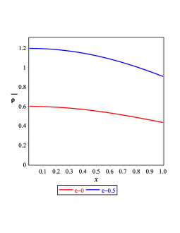
(a)  The density of solution (III)

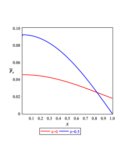
(b)  The radial pressure of solution (III)

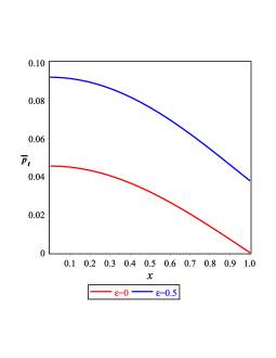
(c)  The transverse pressure of solution (III)

Figure 1: Density, radial and transverse pressures when $\varepsilon=0$ and $\varepsilon=0.5$.

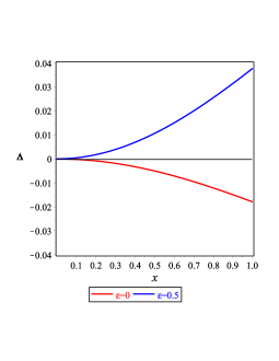
(a)  The anisotropy $\Delta$ of solution (III)

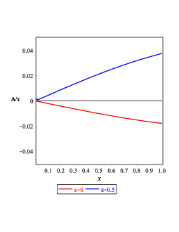
(b)  The anisotropic force $\Delta/\chi$ of solution (III)

Figure 2: Anisotropy $\Delta(\chi)$ and anisotropy force when $\varepsilon=0$ and $\varepsilon=0.5$.

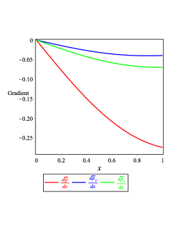
(a)  The gradient of energy-density, radial and tangential pressures of solution (III) when $\varepsilon=0$

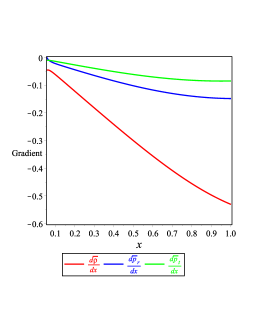
(b)  The gradient of energy-density, radial and tangential pressures of solution (III) when $\varepsilon=0.5$

Figure 3: Gradients of the density, radial, and transverse pressures when $\varepsilon=0$ and $\varepsilon=0.5$

V.2 Causality

To show the behavior of the sound velocities we must calculate the gradient of the energy–density, radial and transverse pressures which take the following form:

$$\tilde{\rho}^{\prime}=-\frac{2e^{-2f_{2}\chi^{2}}}{\chi^{5}}\Bigg{[}4\varepsilon e^{f_{2}\chi^{2}/2}\Big{\{}2-3f_{0}f_{2}\chi^{6}(2f_{0}-5f_{2})-12f_{2}\chi^{4}(f_{0}-f_{2})-\chi^{2}(8f_{0}-11f_{2})\Big{\}}+e^{3f_{2}\chi^{2}/2}\Big{(}2\varepsilon[4+f_{2}\chi^{2}]$$

$$+e^{f_{2}\chi^{2}/2}[\chi^{2}-2\varepsilon]\Big{)}+e^{f_{2}\chi^{2}}\Big{\{}\varepsilon(8f_{2}\chi^{4}[f_{0}-f_{2}]-4[3-f_{0}f_{2}(f_{0}-f_{2})\chi^{6}]+2\chi^{2}[4f_{0}-7f_{2}])-f_{2}\chi^{4}(1-2f_{2}\chi^{2})-\chi^{2}\Big{\}}$$

$$+2\varepsilon\Big{\{}4f_{0}f_{2}(f_{0}-4f_{2})\chi^{6}+8f_{2}\chi^{4}(f_{0}-f_{2})+\chi^{2}(4f_{0}-5f_{2})-1\Big{\}}\Big{]}\,,$$

$$\tilde{p}^{\prime}_{r}=-\frac{2e^{-2f_{2}\chi^{2}}}{\chi^{5}}\Bigg{[}4\varepsilon e^{f_{2}\chi^{2}/2}\Big{\{}4+6f_{0}{}^{2}f_{2}\chi^{6}+9f_{0}f_{2}\chi^{4}+3(2f_{0}+f_{2})\chi^{2}\Big{\}}-4e^{2f_{2}\chi^{2}}(\chi^{2}-2\varepsilon)-e^{f_{2}\chi^{2}}\Big{[}12\varepsilon+\chi^{2}\Big{\{}2f_{0}f_{2}\chi^{4}\Big{(}2f_{0}\varepsilon$$

$$-1\Big{)}+\chi^{4}(12f_{0}f_{2}\varepsilon-f_{2})+6\varepsilon(2f_{0}+f_{2})\Big{\}}\Big{]}-6\varepsilon(1+2f_{0}\chi^{2})(1+f_{2}\chi^{2}[1+2f_{0}\chi^{2}])\Big{]}\,,$$

$$\tilde{p}^{\prime}_{t}=-\frac{2e^{-2f_{2}\chi^{2}}}{\chi^{5}}\Bigg{[}\varepsilon e^{f_{2}\chi^{2}/2}\Big{\{}3f_{0}{}^{2}f_{2}\chi^{8}(2f_{0}-3f_{2})+4f_{0}\chi^{6}(9f_{0}f_{2}-6f_{2}{}^{2}-2f_{0}{}^{2})-12f_{2}\chi^{4}(f_{2}-2f_{0})+\chi^{2}(16f_{0}-11f_{2})-4\Big{\}}$$

$$+\varepsilon e^{3f_{2}\chi^{2}/2}(4+2f_{0}f_{2}\chi^{4}+\chi^{2}[4f_{0}+f_{2}])-2\varepsilon e^{2f_{2}\chi^{2}}+\chi^{2}e^{f_{2}\chi^{2}}[f_{0}f_{2}\chi^{6}(f_{0}-f_{2})+\chi^{4}\{2f_{0}f_{2}\varepsilon(2f_{2}-3f_{0})+f_{2}(3f_{0}-f_{2})-f_{0}{}^{2}\}$$

$$-2\varepsilon\,(f_{2}\chi^{2}+1)(7f_{0}-2f_{2})]+2\varepsilon\{1-4f_{0}{}^{2}f_{2}\chi^{8}(f_{0}-2f_{2})+2f_{0}\chi^{6}(f_{0}{}^{2}+6f_{2}{}^{2}-9f_{0}f_{2})+2f_{2}\chi^{4}(3f_{0}-f_{2})+3\chi^{2}(f_{0}-f_{2})\}\Bigg{]}\,,$$

where $\tilde{\rho}^{\prime}=\frac{d\tilde{\rho}}{d\chi}$, $\tilde{p}^{\prime}_{r}=\frac{d\tilde{p_{r}}}{d\chi}$ and $\tilde{p}^{\prime}_{t}=\frac{d\tilde{p}_{t}}{dx}$. Before graphically analyzing the gradient of the energy-momentum components given by Eq. (V.2) we will write the asymptote form of Eq. (V.2) which yields the following:

$$\tilde{\rho}^{\prime}\approx-f_{2}{}^{2}\chi(4\varepsilon[f_{2}-4f_{0}]+5)+\cdots\,,\qquad\tilde{p}^{\prime}\approx-f_{2}\chi(\varepsilon[6f_{0}f_{2}-8f_{0}{}^{2}-f_{2}{}^{2}]+4f_{0}-f_{2})+\cdots\,,$$

$$\tilde{p}^{\prime}_{t}\approx-\frac{\chi(3f_{2}\varepsilon[6f_{0}f_{2}-8f_{0}{}^{2}-f_{2}{}^{2}]-4f_{0}{}^{2}+12f_{0}f_{2}-4f_{2}{}^{2})}{2}+\cdots\,,\,,$$ (25)

which gives a negative gradient of the energy-momentum components provided that we use the values of $f_{0}$ and $f_{2}$ given by Eq. (23). The behavior of the gradient of density, radial and tangential pressures are shown in Fig. 3 2(a) and 2(b) for $\varepsilon=0$ and $\varepsilon=0.5$.

In order to investigate the causality condition for either the radial or transverse sound speeds $v_{r}{}^{2}$ and $v_{\bot}{}^{2}$, we must show that the values of both of them are less than the speed of light. Using Eq. (V.2) we obtain the asymptotic form of the radial and transverse speeds as the following:

$$v_{r}{}^{2}=\frac{\tilde{p}^{\prime}_{r}}{\tilde{\rho}^{\prime}}\approx\frac{1}{12f_{2}(5-4[4f_{0}-f_{2}]\varepsilon)^{2}}\Big{[}3\varepsilon^{2}[11f_{2}{}^{3}\chi^{2}+2f_{2}{}^{2}(8-19f_{0}\chi^{2})-32f_{0}f_{2}(3+f_{0}\chi^{2})-32f_{0}{}^{2}(f_{0}\chi^{2}-4)](4f_{0}-f_{2})$$

$$-\varepsilon[30f_{0}{}^{3}\chi^{2}+f_{2}{}^{2}(108-196f_{0}\chi^{2})-f_{2}(744f_{0}-592f_{0}{}^{2}\chi^{2})-96f_{0}{}^{2}(2f_{0}\chi^{2}-13)]+60(4f_{0}-f_{2})-16(f_{0}+f_{2})f_{2}\chi^{2}\Big{]}\,,$$

$$v_{t}{}^{2}=\frac{\tilde{p}^{\prime}_{t}}{\tilde{\rho}^{\prime}}\approx\frac{1}{24f_{2}{}^{2}(5-4[4f_{0}-f_{2}]\varepsilon)^{2}}\Big{[}57\varepsilon^{2}f_{2}{}^{5}\chi^{2}+6f_{2}{}^{4}\varepsilon[10\chi^{2}-3\varepsilon(8-47f_{0}\chi^{2})]+4f_{2}{}^{3}[4\chi^{2}-\varepsilon(93-123f_{0}\chi^{2})]$$

$$-f_{2}{}^{2}(96\varepsilon^{2}f_{0}{}^{2}[48-73f_{0}\chi^{2}]+12\varepsilon f_{0}[202+37f_{0}\chi^{2}]-48[6f_{0}\chi^{2}+5])+f_{2}(384\varepsilon^{2}f_{0}{}^{3}[12+5f_{0}\chi^{2}]$$

$$-96\varepsilon f_{0}{}^{2}[41-9f_{0}\chi^{2}]+16f_{0}[45+16f_{0}\chi^{2}])+6f_{0}{}^{3}\varepsilon[131-32f_{0}\chi^{2}]-240f_{0}{}^{2}\Big{]}\,.$$ (26)

Equation (V.2) shows that both $c^{2}>v_{r}{}^{2}>0$ and $c^{2}>v_{t}{}^{2}>0$ utilize the data presented in Eq. (23). The behavior of the radial and tangential speeds of sound are shown in Fig. 4 3(a) and 3(b).

The appearance of the non–vanishing total radial force with different signs in different regions of the fluid is called gravitational cracking when this radial force is directed inward to the inner part of the sphere for all values of the radial coordinate $\chi$ between the center and some value beyond which the force reverses its direction Herrera (1994). In Abreu et al. (2007b) it is stated that a simple requirement for avoiding gravitational cracking is the following $0<v_{r}{}^{2}-v_{t}{}^{2}<c^{2}$. In Fig. 4 3(c) we demonstrate that solution (III) is locally stable against cracking for $\varepsilon=0.5$ but not for $\varepsilon=0$.

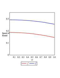
(a)  The radial and transverse speeds of solution (III) when $\varepsilon=0$

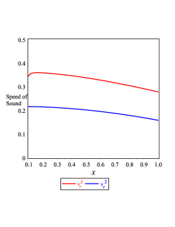
(b)  The radial and transverse speeds of solution (III) when $\varepsilon=0.5$

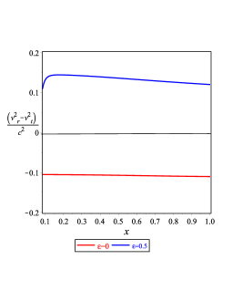
(c)  The cracking of (III) when $\varepsilon=0$ and $\varepsilon=0.5$

Figure 4: Radial, transverse speeds of sound when $\varepsilon=0$ and $\varepsilon=0.5$

V.3 Energy conditions

The energy conditions are an important test for the non–vacuum solution. The dominant energy condition (DEC) leads to the fact that the speed of the energy must be less than that of light. The asymptotic form of the DEC, strong energy condition and weak energy condition take the following forms:

$$DEC\quad\left\{\begin{array}[]{l}\tilde{\rho}-\tilde{p}_{r}\approx 2(2f_{2}-f_{0})-1/2\chi^{2}(2f_{2}{}^{2}+4f_{0}f_{2}-4f_{2}[2f_{0}-f_{2}]+\varepsilon f_{2}[5f_{2}{}^{2}-22f_{0}f_{2}+8f_{0}f_{2}])+\cdots\,,\\ \\ \tilde{\rho}-\tilde{p}_{t}\approx 2(2f_{2}-f_{0})-1/2\chi^{2}(3f_{2}{}^{2}+2f_{0}(f_{0}+f_{2})-4f_{2}[2f_{0}-f_{2}]+\varepsilon f_{2}[11f_{2}{}^{2}-25f_{0}f_{2}+12f_{0}f_{2}])+\cdots\,,\\ \end{array}\right.$$

(30)

$$WEC\quad\left\{\begin{array}[]{l}\tilde{\rho}+\tilde{p}_{r}\approx 2(f_{2}+f_{0})-1/2\chi^{2}(8f_{2}{}^{2}-4f_{0}f_{2}+4f_{2}[2f_{0}-f_{2}]+\varepsilon f_{2}[3f_{2}{}^{2}-10f_{0}f_{2}-8f_{0}f_{2}])+\cdots\,,\\ \\ \tilde{\rho}-\tilde{p}_{t}\approx 2(f_{2}+f_{0})-1/4\chi^{2}(14f_{2}{}^{2}-4f_{0}(f_{0}+f_{2})+8f_{2}[2f_{0}+f_{2}]+\varepsilon f_{2}[5f_{2}{}^{2}-14f_{0}f_{2}-24f_{0}f_{2}])+\cdots\,,\\ \end{array}\right.$$

(34)

$$SEC\quad\tilde{\rho}-\tilde{p}_{r}-2\tilde{p}_{t}\approx 6(f_{2}-f_{0})+\chi^{2}(f_{2}{}^{2}+6(2f_{0}-f_{2})f_{2}-2f_{0}[2f_{2}-f_{0}]+4\varepsilon f_{2}[5f_{0}f_{2}-f_{2}{}^{2}-4f_{0}f_{2}])+\cdots\,.$$

All of the above energy conditions are analytically and graphically satisfied using Eq. (23). Figure 5 shows the behavior of the energy conditions for vanishing and non-vanishing values of the dimensional parameter $\rho$.

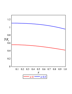
(a)  The DEC, $\tilde{\rho}-\tilde{p}_{r}$, of solution (III)

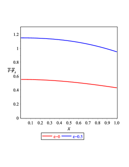
(b)  The DEC, $\tilde{\rho}-\tilde{p}_{t}$, of solution (III)

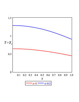
(c)  The WEC, $\tilde{\rho}+\tilde{p}_{r}$ of solution (III)

(d)  The WEC $\tilde{\rho}+\tilde{p}_{t}$ of solution (III)

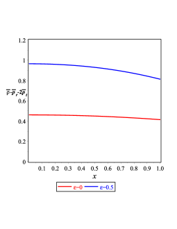
(e)  The SEC $\tilde{\rho}-\tilde{p}_{r}-2\tilde{p}_{t}$ of solution (III)

Figure 5: Energy conditions of solution (III) when $\varepsilon=0$ and $\varepsilon=0.5$

V.4 Mass–radius–relation

The compactification factor $u(r)$ of a compact stellar is defined as the ratio between the mass and radius and is considered as an ingredient role to use to understand the physical properties of the star. From solution (III) we derived the gravitational mass as the following:

$$M(\chi)={\int_{0}}^{\chi}\tilde{\rho(\xi)}\xi^{2}d\xi$$

$$=\frac{1}{36f_{0}{}^{3/2}\chi}\Bigg{[}8\chi\varepsilon\sqrt{6\pi}\,erf(\sqrt{6f_{2}}\,\chi/2)(3f_{2}{}^{2}-2f_{2}{}^{2}-7f_{0}f_{2})+48\varepsilon e^{-3/2f_{2}\chi^{2}}\,\sqrt{f_{2}}(2f_{0}{}^{2}\chi^{2}-f_{2}[3+5f_{0}\chi^{2}])-144\varepsilon f_{2}{}^{3/2}e^{-f_{2}\chi^{2}/2}$$

$$-72\chi\varepsilon f_{2}{}^{2}\sqrt{2\pi}\,erf(\sqrt{2f_{2}}\,\chi/2)-36e^{-f_{2}\chi^{2}}\sqrt{f_{2}}[2\varepsilon f_{0}{}^{2}\chi^{2}+f_{2}(\chi^{2}-2\varepsilon\{3-f_{0}\chi^{2}\})-\varepsilon e^{-f_{2}\chi^{2}}(f_{0}{}^{2}\chi^{2}+f_{2}\{1-4\chi^{2}f_{0}\})]$$

$$+\varepsilon\chi\sqrt{2\pi}\,erf(\sqrt{2f_{2}}\,\chi)[f_{0}{}^{2}+4f_{0}f_{2}-4f_{2}{}^{2}]+36\varepsilon\chi\sqrt{\pi}(f_{0}+2f_{2})(f_{0}+f_{2})\,erf(\sqrt{f_{2}}\,\chi)+36f_{2}{}^{3/2}(\chi^{2}+\varepsilon)\Bigg{]}\,,$$

$$\approx\frac{f_{2}\chi^{3}}{10}(5[2-f_{2}\chi^{2}]-4\varepsilon f_{2}\chi^{2}[f_{2}-4f_{0}])\,,$$ (36)

where $erf(\chi)$ is the error function which is defined as the following:

$$erf(\chi)=\frac{2}{\sqrt{\pi}}\int_{0}^{x}e^{-y^{2}}dy\,.$$ (37)

The compactification factor $u(\chi)$ which is defined as the following:

$$u(\chi)=\frac{M(\chi)}{R}\approx\frac{f_{2}\chi^{3}}{10R}(5[2-f_{2}\chi^{2}]-4\varepsilon f_{2}\chi^{2}[f_{2}-4f_{0}])\,,$$ (38)

where $R$ is the radius of the star and we use Eq. (V.4) in (38). The behavior of the gravitational mass and the compactification factor are plotted in Fig. 6 for $\varepsilon=0$ and $\varepsilon=0.5$.

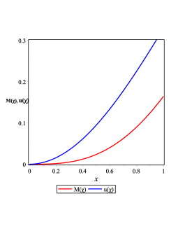
(a)  The gravitational mass of (III) when $\varepsilon=0$

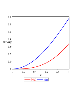
(b)  The compactification factor of (III) when $\varepsilon=0.5$

Figure 6: Gravitational mass and compactification factor of solution (III) when $\varepsilon=0$ and $\varepsilon=0.5$

As Fig. 6 5(a) shows the gravitational mass increases as the radial coordinate does whereas Fig. 6 5(b) displays the compactification factor in direct proportion to the radial coordinate.

V.5 Equation of state

Das et al. Das et al. (2019) showed that the EoS of neutral compact stars in the frame of GR behaves in a linear form however, this study shows that the EoS of solution (III) is not a linear one either for the TEGR or higher order torsion tensor. To rectify this, we define the radial and transverse EoS as the following:

$$\omega_{r}=\frac{\tilde{p}_{r}}{\tilde{\rho}}\approx\frac{2f_{0}-f_{2}}{3f_{2}}-\frac{2f_{2}[f_{0}+f_{2}]-\varepsilon f_{2}[6f_{0}f_{2}-f_{2}{}^{2}-8f_{0}{}^{2}]}{18f_{2}}\chi^{2}+\cdots\,,$$

$$\omega_{t}=\frac{\tilde{p}_{t}}{\tilde{\rho}}\approx\frac{4f_{0}-3f_{2}}{6f_{2}}+\frac{2[f_{2}{}^{2}-8f_{0}f_{2}+6f_{0}{}^{2}]+\varepsilon f_{2}[f_{2}{}^{2}-6f_{0}f_{2}++8f_{0}{}^{2}]}{36f_{2}}\chi^{2}+\cdots\,,$$ (39)

where $\omega_{r}$ and $\omega_{t}$ are the radial and transverse. The behavior of the EoS is shown in Fig 7.

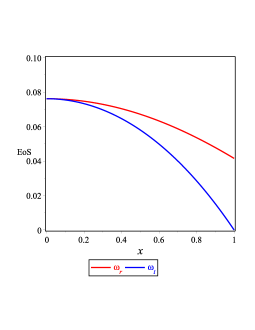
(a)  Radial and tangential EoS when $\varepsilon=0$

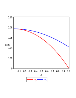
(b)  Radial and tangential EoS when $\varepsilon\neq 0$

Figure 7: Radial and transverse EoS’s of solution (III) for $\varepsilon=0$ and $\varepsilon=-0.01$

As Fig 7 6(a) and 6(b) show that the EoS are also not linear for the case of TEGR, $\varepsilon=0$ or for the higher order torsion. Figure 7 6(a) and 6(b) indicate that for the TEGR case the radial EoS moves to the surface of the star rapidly in comparison to the tangential EoS however for the higher order torsion scalar case the inverse is occurs.

VI Stability of the model

The model’s stability is an important aspect that any physical model must consider. For this we are going to use two different methods, the first being the TOV equation and the second being the adiabatic index.

VI.1 Tolman-Oppenheimer-Volkoff equation

We assume a hydrostatic equilibrium in order to study the stability of solution (III). The TOV equation Tolman (1939); Oppenheimer and Volkoff (1939) which was presented in Ponce de Leon (1993) is as follows:

$$\frac{2[\tilde{p}_{t}-\tilde{p}_{r}]}{\chi}-\frac{M_{g}(\chi)[\tilde{\rho}(\chi)+\tilde{p}_{t}(\chi)]e^{[\alpha(\chi)-\beta(\chi)]/2}}{\chi}-\frac{d\tilde{p}(\chi)}{\chi}=0.$$ (40)

The quantity h $M_{g}(\chi)$ is the gravitational mass of radius $\chi$ which is defined as the following:

$$M_{g}(\chi)=4\pi{\int_{0}}^{\chi}\Big{(}{{\mathcal{T}}_{t}}^{t}-{{\mathcal{T}}_{r}}^{r}-{{\mathcal{T}}_{\theta}}^{\theta}-{{\mathcal{T}}_{\phi}}^{\phi}\Big{)}\chi^{2}e^{[\alpha(\chi)+\beta(\chi)]/2}d\chi=\frac{\chi^{2}\alpha^{\prime}e^{[\beta(\chi)-\alpha(\chi)]/2}}{2}\,,$$ (41)

Using Eqs. (41) in (40) we get

$$\frac{2(\tilde{p}_{t}-\tilde{p}_{r})}{\chi}-\frac{d\tilde{p}_{r}}{d\chi}-\frac{\alpha^{\prime}[\tilde{\varepsilon}(\chi)+\tilde{p}_{r}(\chi)]}{2}=F_{g}+F_{a}+F_{h}=0\,.$$ (42)

The quantities $F_{g}=-\frac{\alpha^{\prime}[\tilde{\rho}+\tilde{p}]}{2}$, $F_{a}=\frac{2(\tilde{p}_{t}-\tilde{p}_{r})}{\chi}$ and $F_{h}=-\frac{d\tilde{p}_{r}(\chi)}{d\chi}$ are the gravitational, anisotropic and hydrostatic forces, respectively. The behavior of the TOV equation of model (III) is shown in Fig. 8 which

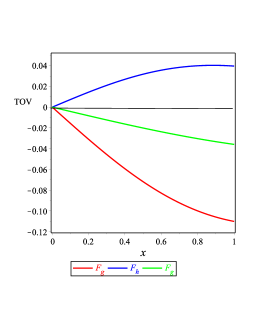
(a)  The TOV Equation when $\varepsilon=0$

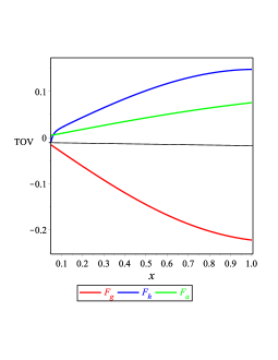
(b)  The TOV Equation when $\varepsilon=0.5$

Figure 8: TOV of solution (III) when $\varepsilon=0$ and $\varepsilon=0.5$

indicates that the anisotropic and gravitational forces are negative and dominated by the hydrostatics force which is positive and keeps the system in static equilibrium in the case of TEGR whereas in the higher order torsion the anisotropic and hydrostatic forces are positive and dominated by the gravitational force which is negative and keeps the system in static equilibrium.

VI.2 The adiabatic index

It is well-known that the adiabatic index is $\gamma$ and defined as Chan et al. (1994); Herrera and Santos (1997)

$$\gamma=\Big{(}1+\frac{\tilde{\rho}}{\tilde{p}}\Big{)}\frac{d\tilde{p}}{d\tilde{\varepsilon}}\,,$$ (43)

which allows us to link the structure of a symmetrically spherical static object and the EoS of the interior solution so that we can investigate its stability Moustakidis (2017). For any interior solution to exhibit stability, it is important that its adiabatic index be greater than $4/3$ Heintzmann and Hillebrandt (1975) and if $\gamma=\frac{4}{3}$ then the isotropic sphere will be in neutral equilibrium. In accordance with the work of Chan et al. Chan et al. (1993), the condition of the stability of a relativistic anisotropic sphere $\gamma>\Gamma$ must be satisfied such that

$$\Gamma=\frac{4}{3}-\left\{\frac{4(\tilde{p}-\tilde{p}_{t})}{3\lvert\tilde{p}^{\prime}\lvert}\right\}_{max}\,.$$ (44)

The behavior of the adiabatic index is shown in Figure 9 which ensures the stability condition of (III).

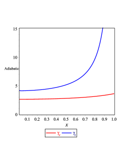
(a)  The adiabatic index of (III) when $\varepsilon=0$

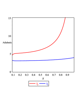
(b)  The adiabatic index of (III) when $\varepsilon=0.5$

Figure 9: Adiabatic index of solution (III) when $\varepsilon=0$ and $\varepsilon=0.5$

Table 1: Values of model parameters when $\varepsilon=0.5$

Pulsar	Mass ($M_{\odot}$)	Radius (km)	$f_{0}$	$f_{1}$	$f_{2}$
J0437-4715	$1.44^{+0.7}_{-0.07}$	$13.6^{+0.9}_{-0.8}$ Reardon et al. (2016); González-Caniulef et al. (2019)	0.2454095942	-0.6438925458	0.39855633
J0030+0451	$1.44^{+0.15}_{-0.16}$	$13.02^{+1.25}_{-1.06}$ Miller et al. (2019)	0.2841372756	-0.7327677384	0.44874578
J0030+0451	$1.34^{+0.15}_{-0.16}$	$12.71^{+1.14}_{-1.19}$Riley et al. (2019)	0.2665730489	-0.6927871908	0.4263174699
EXO 1785 - 248	$1.3^{+0.2}_{-0.2}$	$8.849^{+0.45}_{-0.45}$	0.003403660033	-0.01018791514	0.006784254813
Cen X-3	$1.49^{+0.08}_{-0.08}$	$9.178^{+0.13}_{-0.13}$	0.5216844162	-1.227938771	0.7072044229
RX J 1856 -37	$0.9^{+0.2}_{-0.2}$	$\simeq 6$	0.6103362288	-1.393834058	0.7865648502
Her X-1	$0.85^{+0.15}_{-0.15}$	$8.1^{+0.41}_{-0.41}$	0.2892875212	-0.7441973693	0.4552206652

Table 2: Values of physical quantities when $\varepsilon=0$

Pulsar	$\tilde{\rho}\lvert_{{}_{{}_{\chi=0}}}$	$\tilde{\rho}\lvert_{{}_{{}_{\chi=1}}}$	$\frac{d\tilde{p}_{r}}{d\tilde{\rho}}\lvert_{{}_{{}_{\chi=0}}}$	$\frac{d\tilde{p}_{r}}{d\tilde{\rho}}\lvert_{{}_{{}_{\chi=1}}}$	$\frac{d\tilde{p}_{t}}{d\tilde{\rho}}\lvert_{{}_{{}_{\chi=0}}}$	$\frac{d\tilde{p}_{t}}{d\tilde{\rho}}\lvert_{{}_{{}_{\chi=1}}}$	$(\tilde{\rho}-\tilde{p}_{r}-2\tilde{p}_{t})\lvert_{{}_{{}_{\chi=0}}}$	$(\tilde{\rho}-\tilde{p}_{r}-2\tilde{p}_{t})\lvert_{{}_{{}_{\chi=1}}}$	$z\lvert_{{}_{{}_{\chi=1}}}$
					Millisecond Pulsars
					with White Dwarf
					Companions
J0437-4715	0.598	0.27$\times 10^{-2}$	0	-9$\times 10^{-28}$	-1	-1	0.461	0.81$\times 10^{-2}$	0.039
J0030+0451	0.67	0.3$\times 10^{-2}$	0	-9$\times 10^{-29}$	-1	-1	0.497	0.88$\times 10^{-2}$	0.041
J0030+0451	0.64	0.31$\times 10^{-2}$	0	-9$\times 10^{-26}$	-1	-1	0.48	0.01	0.042
					Pulsars Presenting
					Thermonuclear
					Bursts
EXO 1785 - 248	1.1	0.0064	0	-6$\times 10^{-20}$	-1	-1	0.58	0.02	0.062
Cen X-3	1.06	006	0	-6$\times 10^{-22}$	-1	01	0.58	0.018	0.069
RX J 1856 -37	1.17	0.014	0	-2.1$\times 10^{-9}$	-1	-0.99	0.567	0.0417	0.095
Her X-1	0.64	0.007	0	-2$\times 10^{-10}$	-1	-1	0.48	0.02	0.07

Table 3: Values of physical quantities when $\varepsilon=0.5$

Pulsar	$\tilde{\rho}\lvert_{{}_{{}_{\chi=0}}}$	$\tilde{\rho}\lvert_{{}_{{}_{\chi=1}}}$	$\frac{d\tilde{p}_{r}}{d\tilde{\rho}}\lvert_{{}_{{}_{\chi=0}}}$	$\frac{d\tilde{p}_{r}}{d\tilde{\rho}}\lvert_{{}_{{}_{\chi=1}}}$	$\frac{d\tilde{p}_{t}}{d\tilde{\rho}}\lvert_{{}_{{}_{\chi=0}}}$	$\frac{d\tilde{p}_{t}}{d\tilde{\rho}}\lvert_{{}_{{}_{\chi=1}}}$	$(\tilde{\rho}-\tilde{p}_{r}-2\tilde{p}_{t})\lvert_{{}_{{}_{\chi=0}}}$	$(\tilde{\rho}-\tilde{p}_{r}-2\tilde{p}_{t})\lvert_{{}_{{}_{\chi=1}}}$	$z\lvert_{{}_{{}_{\chi=1}}}$
					Millisecond Pulsars
					with White Dwarf
					Companions
J0437-4715	1.2	0.9	-1.14	0.28	-2.4$\times 10^{-7}$	0.16	0.92	0.86	0.77
J0030+0451	1.3	0.97	1.4	0.29	0.32$\times 10^{-5}$	0.17	0.98	0.93	0.97
J0030+0451	1.3	0.94	9.3	0.28	0.16$\times 10^{-5}$	0.16	0.96	0.9	0.89
					Pulsars Presenting
					Thermonuclear
					Bursts
EXO 1785 - 248	1.7	1.2	0	0.31	3.9$\times 10^{-7}$	0.19	1.1	1.2	2.8
Cen X-3	1.8	1.3	0	0.31	-0.15$\times 10^{-3}$	0.2	1.1	1.2	4.4
RX J 1856 -37	1.8	1.3	0	0.31	1.7$\times 10^{5}$	0.2	1.1	1.2	3.8
Her X-1	1.4	1	0	0.3	0.1	0.2	1	0.95	0.8

VII Discussion and conclusion

In the context of quadratic $f\mathcal{(T)}=\mathcal{T}+\epsilon\mathcal{T}^{2}$ modified gravity and for a KB metric potentials we gave a precise interior solution that has the ability to describe real compact star configurations. The regularity conditions at the origin as well as at the surface of the stellar show that our solution has a good attitude over the stellar structure using the white dwarf companion $PRSJ0437-4715$ . Moreover, we show that the anisotropy of this model has a positive value when the dimensional parameter $\varepsilon\neq 0$ which can be interpreted as a repulsive force. This fact is because the tangential pressure is greater than the radial pressure, i.e., $p_{t}>p_{r}$ Sunzu et al. (2019). When the dimensional parameter $\varepsilon=0$, which is the GR case, we got a negative anisotropy parameter. Furthermore, we study the issue of stability and showed that the derived model is stable against the different forces (gravitational, hydrostatic, anisotropic, and electromagnetic) acting on it. We also calculated the sound of speed and showed that it is consistent with realistic compact stars. Finally, we calculated the adiabatic index of our model and showed that it is also consistent with a realistic physical star. It is worth mention that the adiabatic index presented in Singh et al. (2019) has a negative value that is not consistent with realistic stellar models. The main reason for getting negative adiabatic index Singh et al. (2019) is due to the use of vanishing radial pressure. This indicates, in a clear way, that our assumption of the KB metric potentials (18) are the physical assumption that makes the resulting stellar model in the frame of quadratic $f(T)$ gravitational theory is consistent with real stellar objects.

In this study and for the first time we show the effect of the higher order torsion in modified teleparallel gravitational theories by assuming the form of $f\mathcal{(T)}=\mathcal{T}+\epsilon\mathcal{T}^{2}$. We showed that the effect of the dimensional parameter $\epsilon$ made all the physical parameter consistent with a real stellar pulsar as we discussed in the context of this study. Moreover, we tested our model over a wide range of reported observed values of masses and radii of pulsars are reported in (Tables I, II and III). We show that the fit is good also in these cases.

The present approach can be summarized as follows: we have used a non-diagonal form of the tetrad field that gives a null value of the torsion tensor as soon as the metric potentials approach $1$. This is a crucial condition for any physical tetrad field as reported in various studies DeBenedictis and Ilijic (2016); Abbas et al. (2015); Momeni et al. (2018); Abbas et al. (2015); Chanda et al. (2019); Debnath (2019); Ilijic and Sossich (2018). Moreover, we stress the fact that the tetrad field (9) is a necessary tetrad in the application of any spherically symmetrical interior/exterior solution in the frame of $f(T)$ because it makes the off-diagonal components of the field equations vanishing identically.

Bhatti et al. Bhatti et al. (2018) have discussed the physical features of compact stars using the ansatz of Krori and Barua in the frame of $f(G,{\mathcal{T}})$, where $G$ is the Gauss-Bonnet term and ${\mathcal{T}}$ is the trace of the energy-momentum tensor, showing the behavior of material variables through plots and discussed the physical viability of compact stars through energy conditions. Moreover, in the frame of $f(R)$, discussions of the behavior of different forces, equation of state parameter, measure of anisotropy and TOV equation in the modeling of stellar structures have been carried out. The comparison from their graphical representations provided clear evidence for the realistic and viable $f(R)$ gravity models at both theoretical and the astrophysical scale Yousaf et al. (2017).

We can conclude that the comparison of our exact interior solution with the physical parameters of pulsars gives indications that the model can realistically represent observed systems. Furthermore, the approach can be extended to a large class of metrics and anisotropy if the above physical requirements are satisfied. However, a detailed confrontation with observational data is needed. This will be our forthcoming study.

References

- Weyl (1918) H. Weyl, Sitzungsberichte der Königlich Preußischen Akademie der Wissenschaften (Berlin , 465 (1918).
- Einstein (2006) A. Einstein, “Neue moglichkeit fur eine einheitliche feldtheorie von gravitation und elektrizitat,” (John Wiley and Sons, Ltd, 2006) pp. 322–326, https://onlinelibrary.wiley.com/doi/pdf/10.1002/3527608958.ch37 .
- Mueller-Hoissen and Nitsch (1983) F. Mueller-Hoissen and J. Nitsch, Phys. Rev. D28, 718 (1983).
- O’Raifeartaigh (1997) L. O’Raifeartaigh, The dawning of gauge theory (Princeton Univ. Press, Princeton, NJ, USA, 1997).
- Blagojevic and Hehl (2013) M. Blagojevic and F. W. Hehl, eds., Gauge Theories of Gravitation (World Scientific, Singapore, 2013).
- Hayashi and Shirafuji (1979) K. Hayashi and T. Shirafuji, Phys. Rev. D 19, 3524 (1979).
- Maluf (2013) J. W. Maluf, Annalen der Physik 525, 339–357 (2013).
- Wu and Geng (2012) Y.-P. Wu and C.-Q. Geng, Physical Review D 86 (2012), 10.1103/physrevd.86.104058.
- Li et al. (2011) B. Li, T. P. Sotiriou, and J. D. Barrow, Phys. Rev. D83, 064035 (2011), arXiv:1010.1041 [gr-qc] .
- Shirafuji and Nashed (1997) T. Shirafuji and G. G. L. Nashed, Prog. Theor. Phys. 98, 1355 (1997), arXiv:gr-qc/9711010 [gr-qc] .
- Krssak (2017) M. Krssak, Eur. Phys. J. C77, 44 (2017), arXiv:1510.06676 [gr-qc] .
- Nashed (2003) G. G. L. Nashed, Chaos Solitons Fractals 15, 841 (2003), arXiv:gr-qc/0301008 [gr-qc] .
- Bahamonde et al. (2015) S. Bahamonde, C. G. Boehmer, and M. Wright, Phys. Rev. D92, 104042 (2015), arXiv:1508.05120 [gr-qc] .
- Schwarzschild (1916) K. Schwarzschild, Sitzungsber. Preuss. Akad. Wiss. Berlin (Math. Phys.) 1916, 189 (1916), arXiv:physics/9905030 [physics] .
- Lemaitre (1997) G. Lemaitre, Gen.Rel.Grav. 29, 641 (1997).
- Mak and Harko (2004a) M. K. Mak and T. Harko, Phys. Rev. D 70, 024010 (2004a).
- Mak and Harko (2004b) M. K. Mak and T. Harko, Int. J. Mod. Phys. D13, 149 (2004b), arXiv:gr-qc/0309069 [gr-qc] .
- Ruderman (1972) M. Ruderman, Ann. Rev. Astron. Astrophys. 10, 427 (1972).
- Canuto (1975) V. Canuto, araa 13, 335 (1975).
- Kippenhahn et al. (2013) R. Kippenhahn, A. Weigert, and A. Weiss, Stellar Structure and Evolution; 2nd ed., Astronomy and Astrophysics Library (Springer, Berlin, 2013).
- Tamta and Fuloria (2017) R. Tamta and P. Fuloria, Journal of Modern Physics 08, 1762 (2017).
- Herrera and Santos (1994) L. Herrera and N. O. Santos, Astrophys. J. 438, 308 (1994).
- Letelier (1980) P. S. Letelier, Phys. Rev. D 22, 807 (1980).
- Sawyer (1972) R. F. Sawyer, Phys. Rev. Lett. 29, 382 (1972).
- Usov (2004) V. V. Usov, Phys. Rev. D 70, 067301 (2004).
- Sokolov (1980) A. I. Sokolov, Soviet Journal of Experimental and Theoretical Physics 52, 575 (1980).
- Dev and Gleiser (2003) K. Dev and M. Gleiser, General Relativity and Gravitation 35, 1435 (2003).
- Dev and Gleiser (2002) K. Dev and M. Gleiser, General Relativity and Gravitation 34, 1793 (2002).
- Gleiser and Dev (2004) M. Gleiser and K. Dev, International Journal of Modern Physics D 13, 1389–1397 (2004).
- Ivanov (2010) B. V. Ivanov, International Journal of Theoretical Physics 49, 1236–1243 (2010).
- Schunck and Mielke (2003) F. E. Schunck and E. W. Mielke, Class. Quant. Grav. 20, R301 (2003), arXiv:0801.0307 [astro-ph] .
- Morris and Thorne (1988) M. S. Morris and K. S. Thorne, Am. J. Phys. 56, 395 (1988).
- Cattoen et al. (2005) C. Cattoen, T. Faber, and M. Visser, Class. Quant. Grav. 22, 4189 (2005), arXiv:gr-qc/0505137 [gr-qc] .
- DeBenedictis et al. (2006) A. DeBenedictis, D. Horvat, S. Ilijic, S. Kloster, and K. S. Viswanathan, Classical and Quantum Gravity 23, 2303–“2316 (2006).
- Bowers and Liang (1974) R. L. Bowers and E. P. T. Liang, Astrophys. J. 188, 657 (1974).
- Chan et al. (2003) R. Chan, M. F. A. da Silva, and J. F. Villas da Rocha, Int. J. Mod. Phys. D12, 347 (2003), arXiv:gr-qc/0209067 [gr-qc] .
- Herrera and Santos (1997) L. Herrera and N. O. Santos, Monthly Notices of the Royal Astronomical Society 287, 161 (1997), http://oup.prod.sis.lan/mnras/article-pdf/287/1/161/3165978/287-1-161.pdf .
- Heintzmann and Hillebrandt (1975) H. Heintzmann and W. Hillebrandt, aap 38, 51 (1975).
- (39) “Anisotropic neutron star models: stability against radial and nonradial pulsations. [general relativity theory, newtonian approximation],” .
- Bayin (1982) S. m. c. i. m. c. Bayin, Phys. Rev. D 26, 1262 (1982).
- Krori et al. (1984) K. D. Krori, P. Borgohain, and R. Devi, Canadian Journal of Physics 62, 239 (1984).
- Bondi (1993) H. Bondi, mnras 262, 1088 (1993).
- Bondi (1999) H. Bondi, mnras 302, 337 (1999).
- El Hanafy and Nashed (2016) W. El Hanafy and G. G. L. Nashed, Astrophys. Space Sci. 361, 68 (2016), arXiv:1507.07377 [gr-qc] .
- Barreto (1993) W. Barreto, apss 201, 191 (1993).
- Barreto et al. (2007) W. Barreto, B. Rodríguez, L. Rosales, and O. Serrano, General Relativity and Gravitation 39, 23 (2007).
- Coley and Tupper (1994) A. A. Coley and B. O. J. Tupper, Classical and Quantum Gravity 11, 2553 (1994).
- Martinez et al. (1994) J. Martinez, D. Pavon, and L. A. Nunez, mnras 271, 463 (1994).
- Singh et al. (1995) T. Singh, G. P. Singh, and A. M. Helmi, Il Nuovo Cimento B (1971-1996) 110, 387 (1995).
- Hern??ndez et al. (1999) H. Hernandez, L. A. Nunez, and U. Percoco, Classical and Quantum Gravity 16, 871-896 (1999).
- Harko and Mak (2000) T. Harko and M. Mak, Journal of Mathematical Physics 41, 4752 (2000).
- Nashed and Bamba (2018) G. G. L. Nashed and K. Bamba, JCAP 1809, 020 (2018), arXiv:1805.12593 [gr-qc] .
- Awad and Nashed (2017) A. Awad and G. Nashed, JCAP 1702, 046 (2017), arXiv:1701.06899 [gr-qc] .
- Patel and Mehta (1995) L. K. Patel and N. P. Mehta, Australian Journal of Physics 48, 635 (1995).
- Lake (2004) K. Lake, Phys. Rev. Lett. 92, 051101 (2004).
- Boehmer and Harko (2006) C. G. Boehmer and T. Harko, Classical and Quantum Gravity 23, 6479 (2006).
- Nashed (2011) G. G. L. Nashed, Annalen Phys. 523, 450 (2011), arXiv:1105.0328 [gr-qc] .
- Boehmer and Harko (2007) C. G. Boehmer and T. Harko, Mon. Not. Roy. Astron. Soc. 379, 393 (2007), arXiv:0705.1756 [gr-qc] .
- Esculpi et al. (2007) M. Esculpi, M. Malaver, and E. Aloma, General Relativity and Gravitation 39, 633 (2007).
- Shirafuji et al. (1996) T. Shirafuji, G. G. Nashed, and K. Hayashi, Prog. Theor. Phys. 95, 665 (1996), arXiv:gr-qc/9601044 .
- Khadekar and Tade (2007) G. Khadekar and S. Tade, Astrophysics and Space Science 310, 41 (2007).
- Karmakar et al. (2007) S. Karmakar, S. Mukherjee, R. Sharma, and S. D. Maharaj, Pramana 68, 881 (2007).
- Abreu et al. (2007a) H. Abreu, H. Hernández, and L. A. Núñez, Classical and Quantum Gravity 24, 4631 (2007a).
- IVANOV (2010) B. V. IVANOV, International Journal of Modern Physics A 25, 3975–3991 (2010).
- Herrera et al. (2009) L. Herrera, G. Le Denmat, and N. O. Santos, Phys. Rev. D 79, 087505 (2009).
- Nashed (2008) G. G. L. Nashed, Eur. Phys. J. C54, 291 (2008), arXiv:0804.3285 [gr-qc] .
- Mak and Harko (2003) M. Mak and T. Harko, Proceedings of the Royal Society of London. Series A: Mathematical, Physical and Engineering Sciences 459, 393–408 (2003).
- Sharma and Mukherjee (2002) R. Sharma and S. Mukherjee, Modern Physics Letters A 17, 2535 (2002).
- Maharaj and Maartens (1989) S. D. Maharaj and R. Maartens, General Relativity and Gravitation 21, 899 (1989).
- Chaisi and Maharaj (2006) M. Chaisi and S. D. Maharaj, Pramana 66, 609 (2006).
- Herrera et al. (2008) L. Herrera, J. Ospino, and A. Di Prisco, Phys. Rev. D 77, 027502 (2008).
- Chaisi and Maharaj (2005) M. Chaisi and S. D. Maharaj, General Relativity and Gravitation 37, 1177 (2005).
- Gokhroo and Mehra (1994) M. K. Gokhroo and A. L. Mehra, General Relativity and Gravitation 26, 75 (1994).
- Lake (2009) K. Lake, Phys. Rev. D 80, 064039 (2009).
- V O et al. (2012) T. V O, B. S. Ratanpal, and V. Chackara, International Journal of Modern Physics D 14 (2012).
- Thomas and Ratanpal (2007) V. O. Thomas and B. S. Ratanpal, International Journal of Modern Physics D 16, 1479 (2007).
- Elizalde et al. (2020) E. Elizalde, G. G. L. Nashed, S. Nojiri, and S. D. Odintsov, Eur. Phys. J. C80, 109 (2020), arXiv:2001.11357 [gr-qc] .
- Tikekar and Thomas (2005) R. Tikekar and V. O. Thomas, Pramana 64, 5 (2005).
- Thirukkanesh and Maharaj (2008a) S. Thirukkanesh and S. D. Maharaj, Classical and Quantum Gravity 25, 235001 (2008a).
- Thirukkanesh and Maharaj (2008b) S. Thirukkanesh and S. D. Maharaj, Classical and Quantum Gravity 25, 235001 (2008b).
- Sharma and Ratanpal (2013) R. Sharma and B. S. Ratanpal, Int. J. Mod. Phys. D22, 1350074 (2013), arXiv:1307.1439 [gr-qc] .
- Pandya et al. (2015) D. M. Pandya, V. O. Thomas, and R. Sharma, apss 356, 285 (2015), arXiv:1411.5674 [physics.gen-ph] .
- Bhar et al. (2015) P. Bhar, M. H. Murad, and N. Pant, Astrophysics and Space Science 359, 13 (2015).
- Weitzenböck (1923) R. Weitzenböck, Invariance Theorie (Gronin-gen, 1923).
- Cai et al. (2016) Y.-F. Cai, S. Capozziello, M. De Laurentis, and E. N. Saridakis, Rept. Prog. Phys. 79, 106901 (2016), arXiv:1511.07586 [gr-qc] .
- DeBenedictis and Ilijic (2016) A. DeBenedictis and S. Ilijic, Phys. Rev. D 94, 124025 (2016), arXiv:1609.07465 [gr-qc] .
- Ilijic and Sossich (2018) S. Ilijic and M. Sossich, Phys. Rev. D98, 064047 (2018), arXiv:1807.03068 [gr-qc] .
- Bahamonde et al. (2019) S. Bahamonde, K. Flathmann, and C. Pfeifer, Physical Review D 100 (2019), 10.1103/physrevd.100.084064.
- Roupas and Nashed (2020) Z. Roupas and G. G. Nashed, Eur. Phys. J. C 80, 905 (2020), arXiv:2007.09797 [gr-qc] .
- Nashed et al. (2020) G. G. L. Nashed, A. Abebe, and K. Bamba, arXiv e-prints , arXiv:2002.11471 (2020), arXiv:2002.11471 [physics.gen-ph] .
- Herrera (1994) L. Herrera, Physics Letters A 188, 402 (1994).
- Abreu et al. (2007b) H. Abreu, H. Hernandez, and L. Nunez, Class. Quant. Grav. 24, 4631 (2007b), arXiv:0706.3452 [gr-qc] .
- Das et al. (2019) S. Das, F. Rahaman, and L. Baskey, Eur. Phys. J. C79, 853 (2019).
- Tolman (1939) R. C. Tolman, Phys. Rev. 55, 364 (1939).
- Oppenheimer and Volkoff (1939) J. R. Oppenheimer and G. M. Volkoff, Phys. Rev. 55, 374 (1939).
- Ponce de Leon (1993) J. Ponce de Leon, General Relativity and Gravitation 25, 1123 (1993).
- Chan et al. (1994) R. Chan, L. Herrera, and N. O. Santos, mnras 267, 637 (1994).
- Herrera and Santos (1997) L. Herrera and N. O. Santos, physrep 286, 53 (1997).
- Moustakidis (2017) C. C. Moustakidis, Gen. Rel. Grav. 49, 68 (2017), arXiv:1612.01726 [gr-qc] .
- Chan et al. (1993) R. Chan, L. Herrera, and N. O. Santos, Monthly Notices of the Royal Astronomical Society 265, 533 (1993), http://oup.prod.sis.lan/mnras/article-pdf/265/3/533/3807712/mnras265-0533.pdf .
- Reardon et al. (2016) D. J. Reardon, G. Hobbs, W. Coles, Y. Levin, M. J. Keith, M. Bailes, N. D. R. Bhat, S. Burke-Spolaor, S. Dai, M. Kerr, P. D. Lasky, R. N. Manchester, S. Osłowski, V. Ravi, R. M. Shannon, W. van Straten, L. Toomey, J. Wang, L. Wen, X. P. You, and X. J. Zhu, mnras 455, 1751 (2016), arXiv:1510.04434 [astro-ph.HE] .
- González-Caniulef et al. (2019) D. González-Caniulef, S. Guillot, and A. Reisenegger, mnras 490, 5848 (2019), arXiv:1904.12114 [astro-ph.HE] .
- Miller et al. (2019) M. C. Miller, F. K. Lamb, A. J. Dittmann, S. Bogdanov, Z. Arzoumanian, K. C. Gendreau, S. Guillot, A. K. Harding, W. C. G. Ho, J. M. Lattimer, R. M. Ludlam, S. Mahmoodifar, S. M. Morsink, P. S. Ray, T. E. Strohmayer, K. S. Wood, T. Enoto, R. Foster, T. Okajima, G. Prigozhin, and Y. Soong, apjl 887, L24 (2019), arXiv:1912.05705 [astro-ph.HE] .
- Riley et al. (2019) T. E. Riley, A. L. Watts, S. Bogdanov, P. S. Ray, R. M. Ludlam, S. Guillot, Z. Arzoumanian, C. L. Baker, A. V. Bilous, D. Chakrabarty, K. C. Gendreau, A. K. Harding, W. C. G. Ho, J. M. Lattimer, S. M. Morsink, and T. E. Strohmayer, apjl 887, L21 (2019), arXiv:1912.05702 [astro-ph.HE] .
- Sunzu et al. (2019) J. M. Sunzu, A. K. Mathias, and S. D. Maharaj, Journal of Astrophysics and Astronomy 40, 8 (2019).
- Singh et al. (2019) K. N. Singh, F. Rahaman, and A. Banerjee, (2019), arXiv:1909.10882 [gr-qc] .
- Abbas et al. (2015) G. Abbas, A. Kanwal, and M. Zubair, Astrophys. Space Sci. 357, 109 (2015), arXiv:1501.05829 [physics.gen-ph] .
- Momeni et al. (2018) D. Momeni, G. Abbas, S. Qaisar, Z. Zaz, and R. Myrzakulov, Can. J. Phys. 96, 1295 (2018), arXiv:1611.03727 [gr-qc] .
- Abbas et al. (2015) G. Abbas, S. Qaisar, and A. Jawad, apss 359, 17 (2015), arXiv:1509.06711 [physics.gen-ph] .
- Chanda et al. (2019) A. Chanda, S. Dey, and B. C. Paul, Eur. Phys. J. C79, 502 (2019).
- Debnath (2019) U. Debnath, Eur. Phys. J. C79, 499 (2019), arXiv:1901.04303 [gr-qc] .
- Bhatti et al. (2018) M. Z.-U.-H. Bhatti, M. Sharif, Z. Yousaf, and M. Ilyas, International Journal of Modern Physics D 27, 1850044 (2018).
- Yousaf et al. (2017) Z. Yousaf, M. Sharif, M. Ilyas, and M. Z. Bhatti, Eur. Phys. J. C 77, 691 (2017), arXiv:1710.05717 [gr-qc] .