Precision bound and optimal control in periodically modulated continuous quantum thermal machines

Abstract

We use Floquet formalism to study fluctuations in periodically modulated continuous quantum thermal machines. We present a generic theory for such machines, followed by specific examples of sinusoidal, optimal, and circular modulations respectively. The thermodynamic uncertainty relations (TUR) hold for all modulations considered. Interestingly, in the case of sinusoidal modulation, the TUR ratio assumes a minimum at the heat engine to refrigerator transition point, while the Chopped Random Basis (CRAB) optimization protocol allows us to keep the ratio small for a wide range of modulation frequencies. Furthermore, our numerical analysis suggests that TUR can show signatures of heat engine to refrigerator transition, for more generic modulation schemes. We also study bounds in fluctuations in the efficiencies of such machines; our results indicate that fluctuations in efficiencies are bounded from above for a refrigerator, and from below for an engine. Overall, this study emphasizes the crucial role played by different modulation schemes in designing practical quantum thermal machines.

I Introduction

The necessity of establishing a coherent framework of thermodynamics within the realm of quantum mechanics motivated the field of Quantum Thermodynamics [1, 2, 3]. Such a framework would lead to a deeper understanding of the energetics in the quantum regime, which is crucial in the era of miniaturization of technologies. Moreover, along with the average thermodynamic quantities of interest, the fluctuations about the mean values are necessary for determining the quality of output of such miniature technologies.

In this regard, fluctuation theorems [4, 5, 6, 7] are a remarkable achievement, providing exact mathematical expressions for arbitrary out of equilibrium scenario. Beyond that, recently it has been shown that for out-of-equilibrium systems, there is a limitation to achieving arbitrary precision, which is broadly known as the Thermodynamic Uncertainty Relations (TUR) [8, 9, 10, 11, 12, 13, 14]. Since its first analytical proof for time-continuous classical Markov jump process on a discrete set of states [10], it was subsequently proven for Langevin dynamics with continuous variables [15, 16, 17]. In the meantime, a plethora of studies have been carried out to broaden the regime of its applicability, to include quantum systems. Beyond the standard framework, where the system relaxes to a unique time-independent steady state and the dynamics is time reversal symmetric [18], the original TUR [8, 10] may not hold, thus requiring more general bounds. Specifically, for discrete-time Markov chains [19, 20, 21], time dependent driving [22, 20, 23, 24, 25, 26, 27, 28, 29, 30, 31], underdamped Langevin equation [32, 33, 34, 31], ballistic transport in the presence of magnetic field [27, 35], with measurement and feedback control [36], and arbitrary initial states [37], modified TUR have been put forward. Extensions to the quantum scenario [38, 39, 40, 41, 42, 43, 44, 45] are relatively less explored. In fact, additional complexity that arises due to the genuine quantum features, such as quantum coherence [46, 39, 47, 48, 49, 50, 51, 52] can potentially give rise to violation of the original TUR.

Discovery of TUR have further provided a deep understanding in analysing the thermodynamics of precision for a thermal machine. Along with the power and efficiency to quantify the quality of an engine, the fluctuation around the power output enters into the trade-off relation following the original statement of TUR [8, 9, 10]. This was first shown for steady state classical heat engine connected simultaneously to two baths [13]. As, the TUR does not always hold in its original form, in general such conclusion may not be true for all types of thermal machines. As an example, for cyclic heat engines this trade-off can be overcome [26]. Nevertheless, following this work, generalizations have been put forward in both classical and quantum scenarios. For instance, quantum thermoelectric junctions [39, 46], autonomous quantum thermal machines [48, 52], periodic quantum thermal machines [53, 54, 55, 52] and information driven engines [36] have been studied.

In this paper, we first study a periodically driven continuous quantum thermal machine [56] where the working fluid consists of a minimal two-level system that can work both as an engine and a refrigerator. Employing the techniques of counting field statistics [4] and the Floquet formalism [57, 58, 59, 60], we provide analytic expressions for the currents and fluctuations. Very recently, a novel quantification of fluctuations has been introduced for heat engines [61, 62, 63], defined as the ratio of fluctuation of output work and fluctuation of heat input from the hot bath. Analogous definition has also been provided for refrigerator [62, 63] defined as the ratio of the fluctuation of heat extracted from cold bath and fluctuation of input work. The mathematical form of this quantification is reminiscent of efficiency (co-efficient of performance for refrigerator) giving an essence of the fluctuation for relevant quantities. In general one can define $n-$th order for such quantities taking the ratio of $n-$th order central moments. It was shown that such a quantity is bounded from both below and above for continuous autonomous thermal machines [62]. One advantage for using this quantity is that, as also shown previously for autonomous and discrete thermal machines, such quantity receives a universal upper bound that is solely dependent on the temperature ratio of the cold and hot heat baths. We study the same quantity in the present context. We focus on cases where the qubit is driven by sinusoidal, optimal, and circular modulations. First demonstrating the validity of TUR for each scenario, we find that for such non-autonomous machines, while performing as an engine (refrigerator), the lower (upper) bound is always satisfied whereas we found that the upper (lower) bound is not satisfied at least for one model we considered.

To illustrate further on TUR, in contrast to sinusoidal modulation, the optimized protocol obtained via Chopped Random Basis (CRAB) method allows for reduced TUR ratio for the input (heat current from the hot bath in the engine regime and power in the refrigerator regime) for a wide range of modulation frequencies, whereas the same may not be always true in the case of the output (power output in the engine regime and heat current extracted from the cold bath in the refrigerator regime). Furthermore, for such more generic modulation schemes, we observe that the TUR can show signatures of heat engine to refrigerator transition. Finally, we focus on circular modulation with secular approximation [64, 65]. Combined with the Floquet analysis, we find that the evolution of the diagonal and the off-diagonal elements of the system density matrix are decoupled, leading to Pauli type master equation for the diagonal entries. Consequently, TUR is obeyed for heat currents in this model. In absence of secular approximation, [64, 65] evolution of diagonal and off-diagonal elements of the density matrix may not decouple, thereby leaving a possibility of violating the original TUR.

This paper is organized as follows. In Sec. II, we introduce the techniques of counting field statistics to calculate the currents and fluctuations in periodically driven open quantum systems. In Sec. III, we introduce the model of a minimal continuous quantum thermal machine; we derive the corresponding generalized master equation in Sec. III.1, and discuss the generating function and moments of heat currents and power in Sec. III.2. In Sec. III.3 we present the results for sinusoidal driving. We introduce the CRAB optimization protocol in Sec. III.4.1, and present the optimization results in Sec. III.4.2. Section III.5 deals with circular modulation. Finally, in Sec. IV, we provide a summary of our main results. We provide certain technical details in the appendices.

II Counting field statistics for driven open quantum systems

We write the total Hamiltonian for the system and the baths as

$$H(t)=H_{S}(t)+H_{B}+H_{SB}=H_{0}(t)+H_{SB},$$ (1)

where, $H_{B}=H_{h}+H_{c}$ and, $H_{SB}=H_{Sh}+H_{Sc}=\mathcal{S}\otimes\mathcal{B}_{h}+\mathcal{S}\otimes\mathcal{B}_{c}$. We are considering the situation where the two baths are continuously connected to the system. Here $H_{h}$ ($H_{c})$ denotes the Hamiltonian of the hot (cold) bath; the operators $\mathcal{S}$ and $\mathcal{B}_{j}$ act on the system and the $j(=h,c)$th bath, respectively. We choose the initial state as a product state i.e., $\rho(0)=\rho_{S}(0)\otimes\rho_{B}$, where $\rho_{B}=\rho_{h}\otimes\rho_{c}$ and the reservoirs are prepared in thermal states with respective Hamiltonians $H_{h}$, $H_{c}$ and inverse temperatures $\beta_{h}$, $\beta_{c}$, respectively. The measured observables are the Hamiltonians $H_{h}$ and $H_{c}$. To get the probability distribution of this measurement, we introduce counting field $\chi_{j}$ $(j=h,c)$ to each reservoir. We introduce $\chi\equiv{\{\chi_{h},\chi_{c}\}}$ to denote collectively both the counting variables. The generating function corresponding to the two-point measurement statistics is given by

$$\mathcal{G}(\chi,t)={\rm Tr}_{SB}[\rho(\chi,t)],$$ (2)

where ${\rm Tr}_{SB}$ denotes tracing over both the bath and the system degrees of freedom. The modified density matrix $\rho(\chi,t)$ is given as,

$$\rho(\chi,t)=U(\chi,t)\rho(0)U^{\dagger}(-\chi,t),$$ (3)

with,

$$U(\chi,t)=e^{-i(\chi_{h}H_{h}+\chi_{c}H_{c})/2}U(t)e^{i(\chi_{h}H_{h}+\chi_{c}H_{c})/2}$$ (4)

being the counting field dressed evolution operator. Here $U(t)$ is the unitary evolution operator generated by the total Hamiltonian $H(t)$. Defining, $\rho_{S}(\chi,t)={\rm Tr}_{B}[\rho(\chi,t)]$, we get,

$$\mathcal{G}(\chi,t)={\rm Tr}[\rho_{S}(\chi,t)].$$ (5)

The generating function allows us to evaluate the statistics of energy transferred between system and each reservoir obtained from two point measurement scheme [4]:

$$\langle\Delta E_{j}^{n}\rangle=\frac{\partial^{n}}{\partial{(i\chi_{j})}^{n}}\mathcal{G}(\chi,t)\mid_{\chi=0},$$ (6)

The first order moment $\langle\Delta E_{j}\rangle$ is the heat transferred between the system and $j$-th reservoir. With the spectral decomposition of the bath Hamiltonian as

$$H_{j}=\sum_{m}E_{j}^{k}\ket{k_{j}}\bra{k_{j}}\equiv\sum_{k}E_{j}^{k}P_{j}^{k},$$ (7)

$\langle\Delta E_{j}\rangle$ is defined below, where two projective measurements (the projectors $\{P_{j}^{k}\}$ are defined above) are done on $H_{j}$ at the beginning and at time $t$.

$$\langle\Delta E_{j}\rangle=\sum_{m,n}p_{j}^{m}p_{j}^{nm}(E_{j}^{n}-E_{j}^{m})$$ (8)

where,

$$p_{j}^{nm}={\rm Tr}[P_{j}^{n}U(t)P_{j}^{m}\rho(0)P_{j}^{m}U^{\dagger}(t)P_{j}^{n}]$$ (9)

and $p_{j}^{m}={\rm Tr}[\rho(0)P_{j}^{m}]$ is the probability to measure $E_{j}^{m}$ at $t=0$. In Eq. (9) and in the definition of $p_{j}^{m}$, the projector $P_{j}^{k}$ is understood as $\mathds{1}\otimes P_{j}^{k}$. Now Eq. (6) in turn results in the mean heat current given by,

$$\langle J_{j}(t)\rangle=\frac{d}{dt}\langle\Delta E_{j}\rangle=-i\frac{d}{dt}\frac{\partial}{\partial\chi_{j}}\mathcal{G}(\chi,t)\mid_{\chi=0}.$$ (10)

As per our convention, positive (negative) sign implies current is entering (leaving) the system.

We now proceed to study the dynamics of $\rho(\chi,t)$. Following Eq. (3), the evolution of this modified density matrix is given as [4],

$$\partial_{t}\rho(\chi,t)=-i[H(\chi,t)\rho(\chi,t)-\rho(\chi,t)H(-\chi,t)],$$ (11)

where, $H(\chi,t)=e^{-i(\chi_{h}H_{h}+\chi_{c}H_{c})/2}H(t)e^{i(\chi_{h}H_{h}+\chi_{c}H_{c})/2}$. In the interaction picture one gets (the operators are labelled by tilde)

$$\tilde{\rho}(\chi,t)=U_{0}\rho(\chi,t)U^{\dagger}_{0},$$ (12)

where $U_{0}$ is the unitary operator generated by the Hamiltonian $H_{0}(t)=H_{S}(t)+H_{B}$; the interaction picture Hamiltonian is given by

$$\tilde{H}_{I}(\chi,t)=U_{0}H_{SB}(\chi,t)U_{0}^{\dagger}=\mathcal{\tilde{S}}(t)\otimes(\mathcal{\tilde{B}}_{h}(\chi_{h},t)+\mathcal{\tilde{B}}_{c}(\chi_{c},t))$$ (13)

In the interaction picture, the equation of motion (11) now becomes

$$\partial_{t}\tilde{\rho}(\chi,t)=-i[\tilde{H}_{I}(\chi,t)\tilde{\rho}(\chi,t)-\tilde{\rho}(\chi,t)\tilde{H}_{I}(-\chi,t)],$$ (14)

Next, considering the weak coupling assumption and performing the standard Born-Markov approximation, we arrive at the following master equation

$$\partial_{t}\tilde{\rho}_{S}(\chi,t) =-\int_{0}^{\infty}d\tau{\rm Tr}_{B}[\tilde{H}_{I}(\chi,t)\tilde{H}_{I}(\chi,t-\tau)\tilde{\rho}_{S}(\chi,t)\rho_{B}$$

$$-\tilde{H}_{I}(\chi,t)\tilde{\rho}_{S}(\chi,t)\rho_{B}\tilde{H}_{I}(-\chi,t-\tau)$$

$$-\tilde{H}_{I}(\chi,t-\tau)\tilde{\rho}_{S}(\chi,t)\rho_{B}\tilde{H}_{I}(-\chi,t)$$

$$+\tilde{\rho}_{S}(\chi,t)\rho_{B}\tilde{H}_{I}(-\chi,t-\tau)\tilde{H}_{I}(-\chi,t)],$$ (15)

where we have used ${\rm Tr}_{B}[\tilde{H}_{I}(\chi,t)\rho_{B}]=0$ [66]. The first term on the r.h.s of Eq. (15) can be written as

$$\sum_{j=h,c}\int_{0}^{\infty}d\tau\,\mathcal{\tilde{S}}(t)\mathcal{\tilde{S}}(t-\tau)\tilde{\rho}_{S}(\chi,t)\Phi_{j}(\tau),$$ (16)

where we have ${\rm Tr}_{\tilde{B}_{j}}[\mathcal{\tilde{B}}_{j}(\chi,t_{1})\mathcal{\tilde{B}}_{j}(\eta,t_{2})\rho_{j}]={\rm Tr}_{\tilde{B}_{j}}[\mathcal{\tilde{B}}_{j}(\chi-\eta,t_{1}-t_{2})\mathcal{\tilde{B}}_{j}\rho_{j}]\equiv\Phi_{j}(\chi-\eta,t_{1}-t_{2})$, and $\Phi_{j}(0,t)=\Phi_{j}(t)$. Also, $\mathcal{\tilde{S}}(t)$ is the system operator (in the interaction picture) coming from the interaction Hamiltonian $H_{SB}$. Similarly, evaluating the other terms, we finally have

$$\partial_{t}\tilde{\rho}_{S}(\chi,t) =-\sum_{j=h,c}\int_{0}^{\infty}d\tau[\mathcal{\tilde{S}}(t)\mathcal{\tilde{S}}(t-\tau)\tilde{\rho}_{S}(\chi,t)\Phi_{j}(\tau)$$

$$-\mathcal{\tilde{S}}(t)\tilde{\rho}_{S}(\chi,t)\mathcal{\tilde{S}}(t-\tau)\Phi_{j}(-2\chi,-\tau)$$

$$-\mathcal{\tilde{S}}(t-\tau)\tilde{\rho}_{S}(\chi,t)\mathcal{\tilde{S}}(t)\Phi_{j}(-2\chi,\tau)$$

$$+\tilde{\rho}_{S}(\chi,t)\mathcal{\tilde{S}}(t-\tau)\mathcal{\tilde{S}}(t)\Phi_{j}(-\tau)].$$ (17)

Equation (II) is the generalized master equation for a generic quantum system in presence of arbitrary modulation, the solution of which will provide the required generating function. For later convenience, we introduce the Fourier transform of the correlation functions,

$$\Phi_{j}(-2\chi,\tau)=\frac{1}{2\pi}\int_{-\infty}^{\infty}d\nu e^{-i\nu(\chi+\tau)}G_{j}(\nu).$$ (18)

III A minimal continuous quantum thermal machine

In this section, we focus on the specific case of a thermal machine modelled by a minimal (two-level system) working medium in presence of a periodic modulation [56].

$$H_{S}(t)=H_{S}(t+T);\leavevmode\nobreak\ \leavevmode\nobreak\ \leavevmode\nobreak\ H_{S}(t)=\frac{1}{2}\omega(t)\sigma_{z},$$ (19)

with period $T=2\pi/\Delta$. Additionally, we consider $\mathcal{S}=\sigma_{x}$. One can represent $\mathcal{\tilde{S}}(t)=\sigma_{x}(t)=U^{\dagger}_{S}(t)\sigma_{x}U_{S}(t)$ in the Floquet basis as [67]

$$\tilde{\sigma}_{x}(t) = \sum_{q\in\mathcal{Z}}(\eta(q)e^{-i(\omega_{0}+q\Delta)t}\sigma^{-}+\eta^{*}(q)e^{i(\omega_{0}+q\Delta)t}\sigma^{+}),$$

$$\eta(q) = \frac{1}{T}\int_{0}^{T}\exp\left(i\int^{t}_{0}\left(\omega(s)-\omega_{0}\right)ds\right)e^{-iq\Delta t}dt.$$ (20)

To justify the above equation we refer to the Floquet theory discussed in detail in Appendix A.

We note that the resonance condition $\Delta=\omega_{0}=\frac{1}{T}\int_{0}^{T}\,dt\,\omega(t)$ may result in effective squeezing, as reported in Ref. [68]. Furthermore, experimental constraints may impose a limitation on the maximum frequencies of modulation in any setup. Consequently, in this study we restrict ourselves to low-frequency modulation only, given by $\Delta<\omega_{0}$.

We note that one can consider an autonomous quantum thermal machine as well, which can operate even in the absence of any external periodic modulation [69]. However, such machines are outside the scope of this present work.

III.1 Generalized quantum master equation with counting fields

With the above expansion of $\tilde{\sigma}_{x}(t)$ (see Eq. (III)), we perform a secular approximation for Eq. (II); neglecting the terms with $q\neq q^{\prime}$, the first term of the expression Eq. (II) becomes

$$\frac{1}{2}\sum_{q,j}{|\eta(q)|}^{2} (G_{j}(-\omega_{0}-q\Delta)\sigma^{-}\sigma^{+}\tilde{\rho}_{S}(\chi,t)$$

$$+G_{j}(\omega_{0}+q\Delta)\sigma^{+}\sigma^{-}\tilde{\rho}_{S}(\chi,t)),$$ (21)

where $j=\{h,c\}$. In the above we have neglected the Cauchy principal value and used,

$$\int_{0}^{\infty}d\tau e^{i\tau(y-x)}=\pi\delta(y-x).$$ (22)

Following similar steps and writing for both hot and cold baths, we finally obtain,

$$\partial_{t}\tilde{\rho}_{S}(\chi,t)=\sum_{q,j=\{h,c\}}\mathcal{L}^{q}_{i}(\chi_{j},t)[\tilde{\rho}_{S}(\chi,t)]=$$

$$\sum_{q,j=\{h,c\}}\frac{P_{q}}{2} \Big{(}G_{j}(\omega_{0}+q\Delta)[2e^{-i(\omega_{0}+q\Delta)\chi_{j}}\sigma^{-}\tilde{\rho}_{S}(\chi,t)\sigma^{+}$$

$$-\sigma^{+}\sigma^{-}\tilde{\rho}_{S}(\chi,t)-\tilde{\rho}_{S}(\chi,t)\sigma^{+}\sigma^{-}]$$

$$+G_{j}(-\omega_{0}-q\Delta)[2e^{i(\omega_{0}+q\Delta)\chi_{j}}\sigma^{+}\tilde{\rho}_{S}(\chi,t)\sigma^{-}$$

$$-\sigma^{-}\sigma^{+}\tilde{\rho}_{S}(\chi,t)-\tilde{\rho}_{S}(\chi,t)\sigma^{-}\sigma^{+}]\Big{)},$$ (23)

where $P_{q}={|\eta(q)|}^{2}$ is the weight of the $q-$th Floquet mode. For $\chi=0$, we get back the original master equation without the counting field $\chi$ [4]. We note that here for simplicity we have assumed $\omega_{0}+q\Delta$ is positive for all the significant Floquet modes, which can be the case for modulations with $P_{q}\to 0$ for large $|q|$. A more general case with positive as well as negative $\omega_{0}+q\Delta$ is discussed in Appendix C.

III.2 Generating function, mean currents and fluctuations

With the above generalized master equation (III.1) in hand, we now compute the mean and fluctuations of the heat currents and the output power. Importantly, for the master equation in Eq. (III.1), the evolution of the diagonal and off-diagonal elements are decoupled. As a result, it is enough to consider only the evolution of the diagonal entries of $\tilde{\rho}_{S}(\chi,t)$, where we have noted that the generating function is given by the trace of $\tilde{\rho}_{S}(\chi,t)$ (see Eq. (5)). In the energy eigenbasis, the time evolution of the diagonal entries ${\tilde{\rho}}_{00}(\chi,t)$ and ${\tilde{\rho}}_{11}(\chi,t)$ can be expressed as

$$\begin{pmatrix}\dot{\tilde{\rho}}_{00}(\chi,t)\\ \dot{\tilde{\rho}}_{11}(\chi,t)\end{pmatrix}=\mathcal{L}(\chi)\begin{pmatrix}\tilde{{\rho}}_{00}(\chi,t)\\ \tilde{{\rho}}_{11}(\chi,t)\end{pmatrix},$$ (24)

where the elements of the matrix

$$\mathcal{L}(\chi)=\left[\begin{array}[]{cc}l_{00}&l_{01}^{\chi}\\ l_{10}^{\chi}&l_{11}\end{array}\right]$$ (27)

are

$$l_{00}=-\sum_{q,j}P_{q}G_{j}(\omega_{0}+q\Delta)$$ (28)

$$l_{01}^{\chi}=\sum_{q,j}P_{q}G_{j}(-\omega_{0}-q\Delta)e^{i(\omega_{0}+q\Delta)\chi_{j}}$$ (29)

$$l_{10}^{\chi}=\sum_{q,j}P_{q}G_{j}(\omega_{0}+q\Delta)e^{-i(\omega_{0}+q\Delta)\chi_{j}}$$ (30)

$$l_{11}=-\sum_{q,j}P_{q}G_{j}(-\omega_{0}-q\Delta)$$ (31)

We use the moment generating function Eq. (5) to define the cumulant generating function as,

$$\mathcal{C}(\chi,t)\equiv\log\mathcal{G}=\log{\rm Tr}[\tilde{\rho}_{S}(\chi,t)],$$ (32)

which directly gives us the mean, variance and the higher order cumulants. The steady state is reached in the limit of long times, when the cumulant generating function is dominated by the eigenvalue $\lambda(\chi)$ of $\mathcal{L}(\chi)$ with the largest real part. Therefore one can write [70],

$$\lim_{t\rightarrow\infty}\mathcal{C}(\chi,t)\approx\lambda(\chi)t,$$ (33)

where,

$$\lambda(\chi)=\frac{1}{2}(l_{00}+l_{11})+\frac{1}{2}\sqrt{{(l_{00}+l_{11})}^{2}-4(l_{00}l_{11}-l_{01}^{\chi}l_{10}^{\chi})}.$$ (34)

This in turn results in the mean current in the steady to be given by,

$$\langle J_{j}\rangle=\left.\lim_{t\rightarrow\infty}\frac{d}{dt}\frac{\partial}{\partial(i\chi_{j})}\mathcal{C}(\chi,t)\right|_{\chi=0}=\left.\frac{\partial\lambda(\chi)}{\partial(i\chi_{j})}\right|_{\chi=0,}$$ (35)

$$=\sum_{q}\frac{P_{q}(\omega_{0}+q\Delta)}{w+1}G_{j}(\omega_{0}+q\Delta)[e^{-\beta_{j}(\omega_{0}+q\Delta)}-w].$$ (36)

Here, $w$ is the ratio of the diagonal entries of $\tilde{\rho}_{S}(0,t)$ in the steady state, evaluated setting $\chi=0$ in the Eq. (24) and can be obtained straightforwardly as,

$$\frac{p_{1}^{ss}}{p_{2}^{ss}}\equiv w=\frac{\sum_{q,j}P_{q}G_{j}(\omega_{0}+q\Delta)e^{-\beta_{j}(\omega_{0}+q\Delta)}}{\sum_{q,j}P_{q}G_{j}(\omega_{0}+q\Delta)}=\frac{l_{11}}{l_{00}}.$$ (37)

To arrive at this expression we have used the Kubo-Martin-Schwinger (KMS) boundary condition [71],

$$G_{j}(-\nu)=e^{-\nu}G_{j}(\nu);\leavevmode\nobreak\ \leavevmode\nobreak\ \leavevmode\nobreak\ \nu>0.$$ (38)

and assumed $\left(\omega_{0}+q\Delta\right)>0$ for simplicity. The KMS condition above is the direct consequence of the fact that the bath states are in thermal equilibrium with inverse temperature $\beta_{j}$. For setups with both positive as well as negative $\left(\omega_{0}+q\Delta\right)$, one can consider the same KMS condition (38) to do the analysis, as discussed in Appendix C. Similarly, the current fluctuation is given as,

$${\rm var}(J_{j})=\left.\lim_{t\rightarrow\infty}\frac{d}{dt}\frac{\partial^{2}}{\partial{(i\chi_{j})}^{2}}\mathcal{C}(\chi,t)\right|_{\chi=0}=\left.\frac{\partial^{2}\lambda(\chi)}{\partial(i\chi_{j})^{2}}\right|_{\chi=0},$$

which upon simplification leads to the following expression:

$${\rm var}(J_{j})=\sum_{q}\frac{P_{q}{(\omega_{0}+q\Delta)}^{2}}{w+1}G_{j}(\omega_{0}+q\Delta)[e^{-\beta_{j}(\omega_{0}+q\Delta)}+w]-\frac{2{\langle J_{j}\rangle}^{2}}{\sum_{q,j}P_{q}G_{j}(\omega_{0}+q\Delta)[e^{-\beta_{j}(\omega_{0}+q\Delta)}+1]}$$

$$-\frac{2}{\sum_{q,j}P_{q}G_{j}(\omega_{0}+q\Delta)[e^{-\beta_{j}(\omega_{0}+q\Delta)}+1]}\Big{[}\sum_{q^{\prime},q^{\prime\prime}}P_{q^{\prime}}P_{q^{\prime\prime}}e^{-\beta_{j}(\omega_{0}+q^{\prime}\Delta)}(\omega_{0}+q^{\prime}\Delta)(\omega_{0}+q^{\prime\prime}\Delta)G_{j}(\omega_{0}+q^{\prime}\Delta)G_{j}(\omega_{0}+q^{\prime\prime}\Delta)\Big{]}.$$ (40)

One can use the above results to evaluate the average entropy production rate

$$\langle\dot{S}\rangle=-\beta_{h}\langle J_{h}\rangle-\beta_{c}\langle J_{c}\rangle,$$ (41)

and average output power

$$\langle\mathcal{P}\rangle=-\langle J_{h}\rangle-\langle J_{c}\rangle,$$ (42)

and fluctuations (variance) in power

$${\rm var}(\mathcal{P})={\rm var}(J_{h})+{\rm var}(J_{c})+2\leavevmode\nobreak\ {\rm Cov}(J_{h},J_{c}).$$ (43)

Here the covariance term is given by ${\rm Cov}(J_{h},J_{c})=\langle J_{h}J_{c}\rangle-\langle J_{h}\rangle\langle J_{c}\rangle$, where,

$$\langle J_{h}J_{c}\rangle=\left.\frac{\partial^{2}\lambda(\chi)}{\partial(i\chi_{c})\partial(i\chi_{h})}\right|_{\chi=0}=\frac{1}{l_{00}+l_{11}}\Big{(}\left.\frac{\partial l_{10}^{\chi}}{\partial(i\chi_{c})}\frac{\partial l_{01}^{\chi}}{\partial(i\chi_{h})}+\frac{\partial l_{01}^{\chi}}{\partial(i\chi_{c})}\frac{\partial l_{10}^{\chi}}{\partial(i\chi_{h})}\Big{)}\right|_{\chi_{j}=0}-\frac{2}{l_{00}+l_{11}}\langle J_{h}\rangle\langle J_{c}\rangle;$$

$$\Big{(}\left.\frac{\partial l_{10}^{\chi}}{\partial(i\chi_{c})}\frac{\partial l_{01}^{\chi}}{\partial(i\chi_{h})}+\frac{\partial l_{01}^{\chi}}{\partial(i\chi_{c})}\frac{\partial l_{10}^{\chi}}{\partial(i\chi_{h})}\Big{)}\right|_{\chi_{j}=0}=-\sum_{q^{\prime},q^{\prime\prime}}P_{q^{\prime}}P_{q^{\prime\prime}}e^{-\beta_{h}(\omega_{0}+q^{\prime}\Delta)}(\omega_{0}+q^{\prime}\Delta)(\omega_{0}+q^{\prime\prime}\Delta)G_{h}(\omega_{0}+q^{\prime}\Delta)G_{c}(\omega_{0}+q^{\prime\prime}\Delta)$$

$$-\sum_{q^{\prime},q^{\prime\prime}}P_{q^{\prime}}P_{q^{\prime\prime}}e^{-\beta_{c}(\omega_{0}+q^{\prime\prime}\Delta)}(\omega_{0}+q^{\prime}\Delta)(\omega_{0}+q^{\prime\prime}\Delta)G_{h}(\omega_{0}+q^{\prime}\Delta)G_{c}(\omega_{0}+q^{\prime\prime}\Delta).$$ (44)

Next, we demonstrate the validity of TUR for the heat currents and power for the specific examples of sinusoidal and circular modulations. In addition, we also study the bounds on the ratio of fluctuations for the currents.

III.3 Sinusoidal modulation

In this section we focus on the specific case of sinusoidal modulation:

$$\omega(t)=\omega_{0}+\lambda\,\Delta\,\sin(\Delta t).$$ (45)

Here we assume a weak modulation, quantified by $0\leq\lambda\leq 1$. This assumption allows us to consider only the harmonics $q=0,\pm 1$, with,

$$P_{0}\approx 1-\frac{\lambda^{2}}{2},\leavevmode\nobreak\ P_{\pm 1}\approx\frac{\lambda^{2}}{4},$$ (46)

with the higher order harmonics $P_{q}\approx 0$ for $|q|>1$ in the limit of small $\lambda$. Additionally, we consider the bath spectral functions such that

$$G_{c}(\omega)\approx 0\leavevmode\nobreak\ \text{for}\leavevmode\nobreak\ \omega\geq\omega_{0},\leavevmode\nobreak\ \leavevmode\nobreak\ G_{h}(\omega)\approx 0\leavevmode\nobreak\ \text{for}\leavevmode\nobreak\ \omega\leq\omega_{0}.$$ (47)

The above choice of spectral separation of the baths in Eq. (47) allows the hot (cold) bath to interact with the WM only at higher (lower) energies, which is crucial for the operation of the quantum thermal machine as a heat engine or a refrigerator [56, 72]. This is reminiscent of an Otto cycle, where the WM interacts with the hot (cold) bath only at higher (lower) frequencies [73]. One can use Eqs. (35) - (44) and Eq. (46) to arrive at the mean heat currents, power and their fluctuations (see Appendix B).

With the above setup, one can show that there exists a critical modulation frequency $\Delta\equiv\Delta_{cr}=\omega_{0}\left(T_{h}-T_{c}\right)/\left(T_{h}+T_{c}\right)$, such that the machine works as a heat engine ($\langle J_{h}\rangle>0$, $\langle J_{c}\rangle<0$, $\langle\mathcal{P}\rangle<0$) for $\Delta<\Delta_{cr}$ and as a refrigerator ($\langle J_{h}\rangle<0$, $\langle J_{c}\rangle>0$, $\langle\mathcal{P}\rangle>0$) for $\Delta>\Delta_{cr}$. The power output vanishes while the efficiency approaches the Carnot limit for $\Delta\to\Delta_{\rm cr}$ [56].

We now focus on fluctuations in the operation of the thermal machine described above. To this end, we choose Lorentzian forms for the spectral functions of heat baths described by

$$G_{h}(\omega\geq 0) = \frac{\gamma_{0}\Gamma^{2}\Theta\left(\omega-\omega_{0}-\epsilon\right)}{{(\omega-\omega_{0}-\delta)}^{2}+\Gamma^{2}};$$

$$G_{c}(\omega\geq 0) = \frac{\gamma_{0}\Gamma^{2}\Theta\left(\omega_{0}-\epsilon-\omega\right)}{{(\omega-\omega_{0}-\delta)}^{2}+\Gamma^{2}};$$

$$G_{j}(\omega<0) = G_{j}(\omega\geq 0)e^{-\beta_{h}\omega};\leavevmode\nobreak\ \leavevmode\nobreak\ \leavevmode\nobreak\ j=\{h,c\}$$ (48)

Here, $\gamma_{0}$ is the coupling strength, $\Gamma$ is the width of the spectrum, $\Theta$ denotes the Heaviside function, $\epsilon$ is an infinitesimally small positive constant which ensures that $G_{h}(0\leq\omega<\omega_{0})=G_{c}(\omega>\omega_{0})=0$ (see Eq. (47)), and $\delta>0$ is an energy shift, such that $G_{h}(\omega)$ assumes maximum value at $\omega=\omega_{0}+\delta$.

A consistently performing thermal machine demands low noise-to-signal ratio ${\rm var}\left(\mathcal{J}\right)/\langle\mathcal{J}\rangle^{2}$, for $\mathcal{J}\in\{J_{h},J_{c},\mathcal{P}\}$. On the other hand, a low noise to signal ratio may imply a high entropy production rate $\langle\dot{S}\rangle$, which in turn can result in low efficiency [55]. Consequently, one trade off relation for precision and cost of a thermal machine is the TUR:

$$\mathcal{R}_{j}=\langle\dot{S}\rangle\frac{{\rm var}(\mathcal{J})}{{\mathcal{\langle J\rangle}^{2}}},$$ (49)

where $j=h,c$ or $\mathcal{P}$, for $\mathcal{J}=J_{h},J_{c}$ and $\mathcal{P}$ respectively. For the quantum thermal machine discussed here, the occupation probabilities $p_{0}=\rho_{00}$ and $p_{1}=\rho_{11}$ of the energy eigenstates of $H_{S}$ follow a Pauli-type master equation with time-independent coefficients, as shown in Eq. (24) (setting $\chi=0$). Consequently, one can expect that with the KMS condition, the conventional TUR relation,

$$\mathcal{R}_{j}\geq 2$$ (50)

is satisfied [18, 74, 14, 50].

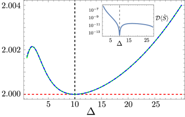
Figure 1: Plot of TUR ratio for heat current $J_{h}$ (green solid line) and power $\mathcal{P}$ (blue dashed-dotted line) with $\Delta$, for sinusoidal modulation. Here, $\omega_{0}=30$, $\beta_{h}=0.005$, $\beta_{c}=0.01$, $\lambda=0.02$, $\Gamma=0.2$, $\delta=3$, and $\gamma_{0}=1$. Critical modulation frequency $\Delta_{cr}=10$, separating the heat engine and the refrigerator regimes are denoted by the vertical black dashed line. The red horizontal dashed line represents the value of the TUR ratio’s lower limit (2). The TUR value saturates to the lower limit at the critical frequency $\Delta_{cr}$. Inset: We plot the difference between the TUR ratio for the power $\mathcal{P}$ and the heat current $J_{h}$, as a function of $\Delta$.

We validate the above inequality (50) numerically, as shown in Fig. 1; here we display the TUR ratio for hot and power currents as a function of $\Delta$. For both cases, the TUR ratio is always lower bounded by the value 2. Note that, for $\Delta<\Delta_{cr}$, the machine works as an engine and for $\Delta>\Delta_{cr}$ the machine works as a refrigerator. As $\Delta$ approaches $\Delta_{cr}$ the TUR value tends to saturate to 2 as at this crossover point all the currents vanish. Furthermore, the expressions for the mean and variance of the currents imply (see Appendix B),

$$\frac{{{\rm{var}}(J_{h})}}{\langle J_{h}\rangle^{2}}=\frac{{{\rm{var}}(J_{c})}}{\langle J_{c}\rangle^{2}},$$ (51)

$$\mathcal{D}:= \frac{{{\rm{var}}(\mathcal{P})}}{\langle\mathcal{P}\rangle^{2}}-\frac{{{\rm{var}}(J_{h})}}{\langle J_{h}\rangle^{2}}=\frac{1}{2}\left(\frac{\omega_{0}^{2}}{\Delta^{2}}-1\right).$$ (52)

Interestingly, the relative fluctuations for both hot and cold currents are the same. As a result, the TUR ratio for both the currents will also be the same and will always be lower bounded by the value 2, i.e.,

$$\langle\dot{S}\rangle\frac{{{\rm{var}}(J_{h})}}{\langle J_{h}\rangle^{2}}=\langle\dot{S}\rangle\frac{{{\rm{var}}(J_{c})}}{\langle J_{c}\rangle^{2}}\geq 2.$$ (53)

The second relation in Eq. (52) leads to some important consequences: In the absence of strong modulation ($\Delta<\omega_{0}$), as $\langle\dot{S}\rangle\geq 0$, one immediately obtains $\mathcal{D}\langle\dot{S}\rangle\geq 0$, implying,

$$\langle\dot{S}\rangle\frac{{{\rm{var}}(\mathcal{P})}}{\langle\mathcal{P}\rangle^{2}}\geq\langle\dot{S}\rangle\frac{{{\rm{var}}(J_{h})}}{\langle J_{h}\rangle^{2}}\geq 2.$$ (54)

The above inequalities (53) and (54) show that reduction in the entropy production rate $\langle\dot{S}\rangle$ comes at the cost of higher noise to signal ratios of the heat currents and power, thus signifying a trade-off between the two. The inset of Fig. 1 shows the quantity $\mathcal{D}\langle\dot{S}\rangle$ in log scale. At the crossover point ($\Delta=\Delta_{\rm cr}$), $\mathcal{D}$ is finite (Eq. (52)), whereas $\langle\dot{S}\rangle$ is zero. Consequently, this gives rise to $\mathcal{D}\langle\dot{S}\rangle$ vanishing at $\Delta=\Delta_{\rm cr}=10$, as also verified numerically in the inset of Fig. 1.

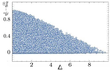
Figure 2: Scatter plot of $\eta_{C}^{2}-\eta^{(2)}_{\rm eng}$ in the engine regime, for sinusoidal modulation. We have considered $10^{5}$ sets of values for $\omega_{0}$, $\beta_{h}$, $\beta_{c}$, and $\Delta$ in the range $(0,10)$, with the constraints $\beta_{h}<\beta_{c}$, and $\Delta<\Delta_{\rm cr}$. For the values of $\Delta$ along the $x$-axis , we plot the corresponding values of $\eta_{C}^{2}-\eta^{(2)}_{\rm eng}$ along the $y$-axis. Here, $\lambda=0.02$, $\Gamma=0.2$, $\delta=3$, and $\gamma_{0}=1$.

We next discuss another recently obtained bound on the ratio of fluctuations of currents and power; following Ref. [62], we define the following quantities:

$$\eta^{(2)}_{\rm eng}=\frac{{{\rm{var}}(\mathcal{P})}}{{\rm var}(J_{h})},\leavevmode\nobreak\ \leavevmode\nobreak\ \text{for engine};$$

$$\eta^{(2)}_{\rm ref}=\frac{{{\rm{var}}(J_{c})}}{{\rm var}(\mathcal{P})},\leavevmode\nobreak\ \leavevmode\nobreak\ \text{for refrigerator}.$$ (55)

Based on Onsager’s reciprocity relations in the linear response regime for autonomous continuous machines, it was recently shown that $\eta^{(2)}$ is bounded from both above as well as below, as [62]

$$\langle\eta\rangle_{\rm eng}^{2}\leq\eta^{(2)}_{\rm eng}\leq\eta_{C}^{2},\leavevmode\nobreak\ \leavevmode\nobreak\ \text{for engine};$$

$$\langle\eta\rangle_{\rm ref}^{2}\leq\eta^{(2)}_{\rm ref}\leq{\left(\frac{1-\eta_{C}}{\eta_{C}}\right)}^{2}=\eta_{R}^{2},\leavevmode\nobreak\ \leavevmode\nobreak\ \text{for refrigerator}.$$ (56)

Here $\langle\eta\rangle_{\rm eng}=\mathcal{\langle P\rangle}/\langle J\rangle_{h}$ and $\langle\eta\rangle_{\rm ref}=\langle J\rangle_{c}/\mathcal{\langle P\rangle}$ denote the efficiency of the engine and the coefficient of performance for the refrigerator, respectively. $\eta_{C}=1-\frac{\beta_{h}}{\beta_{c}}$ is the Carnot efficiency. Knowledge about such bounds in the present context is crucial for designing optimal non-autonomous continuous quantum thermal machines beyond linear response. We therefore now assess the validity of these bounds for our periodically driven continuous quantum thermal machine setup.

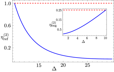
Figure 3: Plot of $\eta_{\rm ref}^{(2)}$ with $\Delta$, for sinusoidal modulation. Here, $\omega_{0}=30$, $\beta_{h}=0.005$, $\beta_{c}=0.01$, $\lambda=0.02$, $\Gamma=0.2$, $\delta=3$, and $\gamma_{0}=1$. Critical modulation frequency $\Delta_{cr}=10$. The horizontal red dashed line represents $\eta_{R}^{2}=1$. Inset: We plot $\eta_{\rm eng}^{(2)}$ with $\Delta$ for the same parameter values. The red dashed horizontal line represents $\eta_{C}^{2}=0.25$.

Following the above expressions in Eq. (51) and Eq. (52) for relative fluctuations in the engine regime, we arrive at the following relations:

$$\eta^{(2)}_{\rm eng}=\frac{{{\rm{var}}(\mathcal{P})}}{{\rm var}(J_{h})}>\frac{\langle\mathcal{P}\rangle^{2}}{\langle J_{h}\rangle^{2}}=\langle\eta\rangle_{\rm eng}^{2},$$ (57)

therefore implying that the lower bound gets respected. Note that, as in this case, the equality in the lower bound is never achieved in the engine regime $\Delta<\omega_{0}$. Next, in the refrigerator regime, we find,

$$\eta^{(2)}_{\rm ref}=\frac{{{\rm{var}}(J_{c})}}{{\rm var}(\mathcal{P})}<\frac{\langle J_{c}\rangle^{2}}{\langle\mathcal{P}\rangle^{2}}=\langle\eta\rangle_{\rm ref}^{2}\leq\eta_{R}^{2},$$ (58)

thus signifying the violation of the lower bound but always validating the upper bound. Note that, for finite-time discrete quantum Otto cycle, a setup that is in stark contrast to the present situation, similar observations were pointed out [63].

For the upper bound in the engine regime, we provide a scatter plot and observe the validity of the corresponding bound. In Fig. 2, we plot the difference between $\eta_{C}^{2}$ and $\eta_{\rm eng}^{(2)}$ with $\Delta$ for $10^{5}$ randomly generated set of parameters within the range $(0,10)$, satisfying the constraints $\beta_{h}<\beta_{c}$ and $\Delta<\Delta_{\rm cr}$, for each point. From the figure it is evident that the difference is always positive, implying the validity of the upper bound in the engine regime. For the refrigerator regime, we have already argued in Eq. (58) that the upper bound is respected. It saturates in the limit when the entropy production rate vanishes, as illustrated in Fig. 3, the upper bound saturates for both engine and refrigerator case in the limit of zero power which corresponds to $\Delta\rightarrow\Delta_{\rm cr}$. We emphasize that the above results are specific to sinusoidal modulation. In Sec. III.4 we show that in case of more generic modulation schemes, the lower bound for engine, and the upper bound for refrigerator always remain robust.

III.4 TUR minimization through optimal control

III.4.1 CRAB Optimization Protocol

The sinusoidal modulation discussed above does not guarantee optimal operation. We, therefore now focus on the CRAB optimization protocol [75, 76, 77], aimed at minimizing the TUR ratio for heat currents and power. The CRAB optimization scheme has proven to be highly successful in several theoretical [78, 79], as well as experimental [80, 81] works, and can be modeled as a generic periodic modulation of $\omega(t)$ expressed as a truncated Fourier series:

$$\omega(t) = \omega_{0}+\frac{\mu}{2NR(t)}\sum_{n=1}^{N}\Big{[}a_{n}\cos\left(\frac{2\pi nt}{T}\right)$$ (59)

$$+ b_{n}\sin\left(\frac{2\pi nt}{T}\right)\Big{]},$$

where the Hamiltonian is given by Eq. (19). Here the positive integer $N$ denotes the total number of frequencies considered, while $T$ is the time period of modulation. The function $R(t)\rightarrow\infty$ for $t=0$ and $t=T$, while $R(t)=1$ for intermediate times, such that $\omega(t)=\omega_{0}$ at the beginning and end of a cycle. We numerically optimize the Fourier coefficients $-1\leq a_{n}\leq 1$, $-1\leq b_{n}\leq 1$, so as to optimize a relevant cost function, subject to certain constraints, such as the strength of control $\mu$. In the present case, we perform the above optimization protocol in order to minimize the TUR ratio $\mathcal{R}_{j}$, as defined in Eq. (49), for various currents and power (see also Appendix C). For the optimization, we choose the same spectral function as done for the sinusoidal case [Eq. (48)].

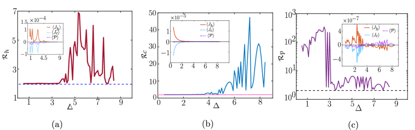
Figure 4: Plot showing the TUR ratio (a) $\mathcal{R}_{h}$ for the hot current $J_{h}$, (b) $\mathcal{R}_{c}$ for the cold current $J_{c}$ and (c) $\mathcal{R}_{p}$ for the output power $\mathcal{P}$, as a function of $\Delta$, for the CRAB modulation Eq. (59). As expected, $\mathcal{R}_{j}$ is bounded from below by $\mathcal{R}_{j}=2$ for all values of $\Delta$, for $j=h,c$, and $\mathcal{P}$. The insets show the variation of the mean energy currents $\langle J_{h}\rangle,\langle J_{c}\rangle$ and the mean power $\langle\mathcal{P}\rangle$ as functions of $\Delta$. As seen in (a) and (b), through CRAB optimization, one can have $\mathcal{R}_{h,c}\to 2^{+}$ at non-zero output power, for a wide range of $\Delta$. The parameters are fixed as $\omega_{0}=30$, $\beta_{h}=0.005$, $\beta_{c}=0.01$, $\Gamma=0.2$, $\delta=3$, $\gamma_{0}=1$, $\mu=1$, and $N=10$.

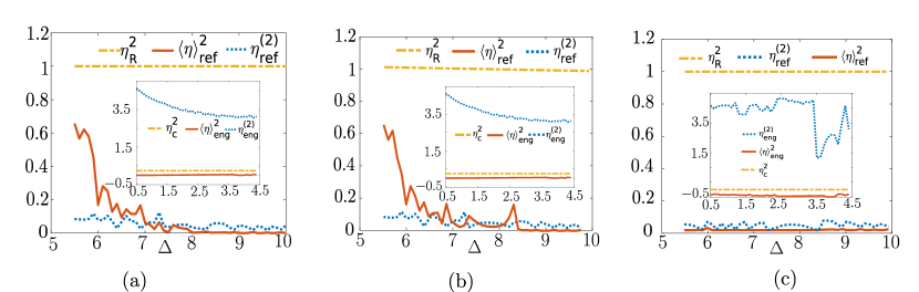
Figure 5: Plot of $\langle\eta\rangle_{\rm ref}^{2}$, $\eta_{\rm ref}^{(2)}$, and $\eta_{R}^{2}$ with $\Delta$, in the refrigerator regime. In Fig. 5(a), for any $\Delta$, we have considered the pulse used in Fig. 4(a), aimed at minimizing $\mathcal{R}_{h}$ for that particular $\Delta$. Similarly, in Fig. 5(b) and Fig. 5(c) we have considered the pulse used in Fig. 4(b) and Fig. 4(c), respectively. The insets show the plots for of $\eta^{(2)}_{\rm eng},\langle\eta\rangle_{\rm eng}^{2}$, and $\eta_{C}^{2}$ with $\Delta$ in the heat engine regime. We observe that in all cases the lower bound for the engine i.e., $\eta^{(2)}_{\rm eng}\geq\langle\eta\rangle^{2}$ and the upper bound for the refrigerator i.e., $\eta^{(2)}_{\rm ref}\leq\eta_{R}^{2}$ always remain valid.

III.4.2 Optimization and Result

For any modulation frequency $\Delta=2\pi/T$, we numerically optimize the coefficients $\{a_{n}\},\{b_{n}\}$ through pattern search optimization method, in order to minimize the TUR ratio for $J_{h}$ ($\mathcal{R}_{h}$, see Fig. 4(a)), $J_{c}$ ($\mathcal{R}_{c}$, see Fig. 4(b)) and $\mathcal{P}$ ($\mathcal{R}_{\mathcal{P}}$, see Fig. 4(c)) for that $\Delta$. Here $n=1,2,3,...,N$, and we consider a cutoff $N=10$. The optimal set of coefficients $\{a_{n},b_{n}\}_{\Delta}$ defines the periodic modulation with the corresponding $\Delta$. As seen in Fig. 4(a), Fig. 4(b), and Fig. 4(c) the TUR ratio $\mathcal{R}_{j}\geq 2$ for all $\Delta$, for $j=h,c$, and $\mathcal{P}$. Furthermore, we note that in the case of the sinusoidal modulation, the TUR ratio was minimal at the crossover point where all the currents were zero (see Fig. 3). However the numerical optimization scheme suggests one can use the CRAB protocol to get a small TUR ratio ($\mathcal{R}_{j}\to 2^{+}$) for $J_{h}$ and $J_{c}$ at non-zero output power for a wide range of modulation frequencies $\Delta$ in the heat engine regime ($\langle J_{h}\rangle>0,\langle J_{c}\rangle<0,\langle\mathcal{P}\rangle<0$), thus highlighting the advantage of performing CRAB optimization. Moreover, a noteworthy observation in Fig. 4(a) is that in the heat engine regime $(0<\Delta\lesssim 4)$, the TUR ratio for the input i.e., $\mathcal{R}_{h}$ can be reduced to small values and can saturate the TUR bound through optimal control, whereas the same may not be always true in case of the output heat current $\mathcal{J}_{c}$ in the refrigerator regime $\Delta\gtrsim 4$, as shown by $\mathcal{R}_{c}$ in Fig. 4(c). This may be attributed to small values of $\langle\mathcal{J}_{c}\rangle$ in the refrigerator regime (cf. inset of Fig. 4(b)), as compared to larger values of $\langle\mathcal{J}_{h}\rangle$ in the heat engine regime (cf. inset of Fig. 4(a)). A similar behavior is also noticed for the TUR ratio $\mathcal{R}_{p}$ as well. Furthermore, the contrasting behaviors of TUR in the heat engine ($0<\Delta\lesssim 4$) and the refrigerator ($\Delta\gtrsim 4$) regimes in Figs. 4(a), 4(b) and 4(c) suggest that TUR can exhibit signatures of heat engine to refrigerator transition for more generic modulation schemes. We next study the bounds in the fluctuations in efficiencies in Figs. 5(a)-5(c), for the pulses used in Figs. 4(a)- 4(c). As seen in Fig. 5(a), the lower bound in the refrigerator regime, as suggested by Eq. (56), is violated for a wide range of $\Delta$, while the upper bound i.e., $\eta^{(2)}_{\rm ref}\leq\eta_{R}^{2}$ always remains valid. This is in agreement with our observation for the case of sinusoidal modulation (see Eq. (58)). Interestingly, in the engine regime, a completely opposite trend is observed for the bounds. We observe that the lower bound i.e., $\eta^{(2)}_{\rm eng}\geq\langle\eta\rangle^{2}$ always remains valid, as was also the case for sinusoidal driving (see Eq. (57)); in contrast, now the upper bound gets violated for this optimal driving scenario. In summary, in all the cases we observe the validity of the lower bound for the engine and the upper bound for the refrigerator. This is in stark contrast to autonomous quantum thermal machines, where the upper and lower bounds for fluctuations have been shown to hold in the linear response regime [62, 63]. On the other hand, the absence of linear response and the presence of external periodic modulation invalidates those bounds in the present context. These results indicate crucial differences in the nature of the fluctuations for currents in the engine and the refrigerator regimes, as well as in non-autonomous continuous thermal machines in comparison to their autonomous counterparts. A comparative analysis of fluctuations and optimization in continuous and stroke thermal machines may yield interesting results as well [26]. Furthermore, they emphasize the importance of rigorous studies regarding bounds of fluctuations in generic quantum thermal machines.

III.5 Circular modulation

We next consider circular modulation, given by:

$$H_{S}(t)=\frac{\omega_{0}}{2}\sigma_{z}+g(\sigma^{-}e^{i\Omega t}+\sigma^{+}e^{-i\Omega t}).$$ (60)

In contrast to the sinusoidal and the CRAB modulations discussed above, here $\left[H_{\rm S}(t),H_{\rm S}(t^{\prime})\right]$ may not commute for $t\neq t^{\prime}$. This non-commutative property of the system Hamiltonian can lead to quantum friction, thereby changing the qualitative nature of the thermal machine [82]. Consequently, such modulation (60) can play an important role in understanding the role of fluctuations in continuous minimal quantum thermal machines. Moreover, as we show below, the model considered here results in the realization of a heat accelerator, thereby allowing us to extend our analysis to periodically modulated continuous thermal machines operating beyond the heat engine or refrigerator regimes [83].

One can refer to the Floquet analysis in Appendix A and Appendix D to arrive at the following generalized master equation [65, 84], starting from Eq. (II),

$$\dot{\tilde{\rho}}_{\alpha\beta}= -\sum_{j=h,c}\int_{0}^{\infty}d\tau\Phi_{j}(\tau)\sum_{m,n,l,l^{\prime}}e^{i(\epsilon_{\alpha}-\epsilon_{m})t}e^{i(\epsilon_{m}-\epsilon_{n})(t-\tau)}e^{il\Omega t}e^{il^{\prime}\Omega(t-\tau)}S_{\alpha m}^{l}S_{mn}^{l^{\prime}}\rho_{n\beta}$$

$$+\sum_{j=h,c}\int_{0}^{\infty}d\tau\Phi_{j}(-2\chi,-\tau)\sum_{m,n,l,l^{\prime}}e^{i(\epsilon_{\alpha}-\epsilon_{m})t}e^{i(\epsilon_{n}-\epsilon_{\beta})(t-\tau)}e^{il\Omega t}e^{il^{\prime}\Omega(t-\tau)}S_{\alpha m}^{l}S_{n\beta}^{l^{\prime}}\rho_{mn}$$

$$+\sum_{j=h,c}\int_{0}^{\infty}d\tau\Phi_{j}(-2\chi,\tau)\sum_{m,n,l,l^{\prime}}e^{i(\epsilon_{n}-\epsilon_{\beta})t}e^{i(\epsilon_{\alpha}-\epsilon_{m})(t-\tau)}e^{il\Omega(t-\tau)}e^{il^{\prime}\Omega t}S_{\alpha m}^{l}S_{n\beta}^{l^{\prime}}\rho_{mn}$$

$$-\sum_{j=h,c}\int_{0}^{\infty}d\tau\Phi_{j}(-\tau)\sum_{m,n,l,l^{\prime}}e^{i(\epsilon_{m}-\epsilon_{n})(t-\tau)}e^{-i(\epsilon_{n}-\epsilon_{\beta})t}e^{il\Omega(t-\tau)}e^{il^{\prime}\Omega t}S_{mn}^{l}S_{n\beta}^{l^{\prime}}\rho_{\alpha m}.$$ (61)

where, $\epsilon_{\alpha}$’s are the eigenvalues of the Floquet Hamiltonian $H_{F}$, and all the indices are integers (Appendix A). We here perform the secular approximations for the above master equation; we neglect the fast oscillating terms of the form $e^{il\Omega t}$ (for $l\neq 0$). Additionally, we also neglect the terms of the form of $e^{i(\epsilon_{\alpha}-\epsilon_{\beta})t}$ (for $\alpha\neq\beta$) [64, 65]. As a result of the secular approximation, evolution of diagonal and off-diagonal terms of the above master equation get decoupled, and we get a conventional Pauli rate equation with the diagonal entries containing time-independent transition rates. We therefore have,

$$\begin{pmatrix}\dot{\tilde{\rho}}_{00}(\chi,t)\\ \dot{\tilde{\rho}}_{11}(\chi,t)\end{pmatrix}=\begin{pmatrix}l_{00}^{\chi}&l_{01}^{\chi}\\ l_{10}^{\chi}&l_{11}^{\chi}\end{pmatrix}\begin{pmatrix}\tilde{\rho}_{00}(\chi,t)\\ \tilde{\rho}_{11}(\chi,t)\end{pmatrix},$$ (62)

where,

$$l_{00}^{\chi}= {|S_{11}^{1}|}^{2}\sum_{j=h,c}\left[G_{j}(\Omega)(e^{-i\Omega\chi_{j}}-1)+G_{j}(-\Omega)(e^{i\Omega\chi_{j}}-1)\right]$$

$$-{|S_{12}^{1}|}^{2}\sum_{j=h,c}G_{j}(\Omega\!-\!\Omega_{R})\!-\!{|S_{21}^{1}|}^{2}\sum_{j=h,c}G_{j}(-\Omega\!-\!\Omega_{R})$$ (63)

$$l_{01}^{\chi}= {|S_{12}^{1}|}^{2}\sum_{j=h,c}G_{j}(-\Omega+\Omega_{R})e^{-i(-\Omega+\Omega_{R})\chi_{j}}$$

$$+{|S_{21}^{1}|}^{2}\sum_{j=h,c}G_{j}(\Omega+\Omega_{R})e^{-i(\Omega+\Omega_{R})\chi_{j}}$$ (64)

$$l_{10}^{\chi}= {|S_{12}^{1}|}^{2}\sum_{j=h,c}G_{j}(\Omega-\Omega_{R})e^{-i(\Omega-\Omega_{R})\chi_{j}}$$

$$+{|S_{21}^{1}|}^{2}\sum_{j=h,c}G_{j}(-\Omega-\Omega_{R})e^{i(\Omega+\Omega_{R})\chi_{j}}$$ (65)

$$l_{11}^{\chi}= {|S_{22}^{1}|}^{2}\sum_{j=h,c}\left[G_{j}(\Omega)(e^{-i\Omega\chi_{j}}-1)+G_{j}(-\Omega)(e^{i\Omega\chi_{j}}-1)\right]$$

$$-{|S_{12}^{1}|}^{2}\sum_{j=h,c}G_{j}(-\Omega+\Omega_{R})-{|S_{21}^{1}|}^{2}\,\sum_{j=h,c}G_{j}(\Omega+\Omega_{R})$$ (66)

As before, we are interested in the long time limit and computing the steady-state currents and fluctuations. We once again use the properties of the cumulant generating function (Eq. (33), Eq. (35) and Eq. (III.2)) to calculate the mean and variance of the heat currents and the power and check the validity of the inequality (50).

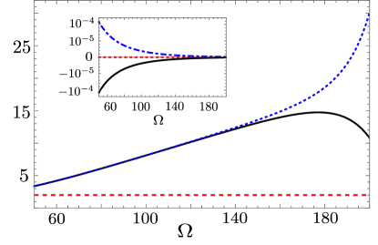
Figure 6: Plot of TUR ratio for hot (black solid) and cold (blue dotted line) bath currents as a function of driving frequency $\Omega$, for circular modulation. Here, $\omega_{0}=25$, $\beta_{h}=0.01$, $\beta_{c}=0.06$, $g=0.02$, $\Gamma=0.2$, $\delta=3$, and $\gamma_{0}=1$. The dashed horizontal red line represents the value of the lower bound (2) of TUR ratio. The inset shows the hot (blue dashed-dotted), cold (black solid line) bath currents, and the power (red dotted line).

Here we consider a Lorentzian bath spectrum for both the hot bath and the cold bath as follows

$$G_{j}(\omega)=\frac{\gamma_{0}\Gamma^{2}}{{(\delta-\omega)}^{2}+\Gamma^{2}},$$ (67)

$$G_{j}(-\omega)=G_{j}(\omega)e^{-\beta_{j}\omega},\leavevmode\nobreak\ \leavevmode\nobreak\ \leavevmode\nobreak\ j=\{h,c\}$$ (68)

where the parameters are defined after Eq. (48); $G_{h}(\omega)$ and $G_{c}(\omega)$ assume maxima at $\omega=\delta.$ As shown in the inset of Fig. 6, the machine always works as a heat accelerator for all values of $\Omega$. Thermal machines working on time scales in which the typical Born-Markov approximations do not hold may lead to different possibilities [85, 86]. As we don’t get any useful work from this machine, we are not interested in the fluctuations of power and all the precision bounds introduced in the previous section. Instead, we solely focus on the TUR ratio for hot and cold heat currents. As shown in Fig. 6, the inequality (50) is satisfied in this scenario. This can be expected as due to the secular approximation, the diagonal and off-diagonal elements of the system density matrix evolve independently in time which results in a Pauli-type master equation with time-independent coefficients for the occupation probabilities. This, along with the local detailed balance condition, results in the condition $\mathcal{R}\geq 2$ [74, 18, 14, 50]. Unlike the case of sinusoidal modulation, the noise to signal ratio is not the same for hot and cold currents in case of circular modulation, as can be seen from Fig. 6. For sinusoidal modulation, the spectral separation condition Eq. (47) results in the difference between noise to signal ratio for the hot and cold current to vanish, as shown in Appendix B. However, the same is not true in case of circular modulation.

IV Conclusion

In this paper, we discuss periodically driven continuous heat machines from the Floquet perspective. Employing the counting field statistics approach, we compute the steady-state heat currents and the associated fluctuations for generic periodically driven continuous thermal machines with the two-level systems as a working medium. We have exemplified our theory using the specific cases of sinusoidal, CRAB optimized and circular modulations. We have analyzed different precision bounds and trade-offs with these fluctuations; specifically, we find that TUR is satisfied for the machines considered here. One can operate the sinusoidally modulated thermal machine as a heat engine, or a refrigerator, depending on the frequency of modulation, thus motivating us to study the fluctuations in this model in greater detail. Interestingly, our analysis shows that the noise-to-signal ratio for the heat currents from the hot and the cold baths are equal in case of sinusoidal modulation. Moreover, one can define a parameter to quantify the fluctuations in efficiency, which appears to be bounded from both above and below in the heat engine regime, while the existence of an equivalent lower bound is not clear in the case of the refrigerator regime. Note that, similar phenomena was observed recently for a discrete stroke heat machine as well [63].

We have used CRAB optimization protocol to minimize TUR and study the bounds in the fluctuations of efficiency. As expected, the TUR is always bounded from below by two. Numerical analysis suggests that (i) in the heat engine regime, one can use optimal control to operate the thermal machine with minimum TUR ($=2$) for the heat currents, at non-zero power output; (ii) one can reduce the TUR ratio for the input (heat current absorbed from the hot bath in the engine regime and power in the refrigerator regime) to small values through optimal control, whereas the same may not be always true in case of the output (power output in the engine regime and heat current extracted from the cold bath in the refrigerator regime) (see Fig. 4); (iii) the lower (upper) bound for the fluctuations in efficiency is always satisfied in the heat engine (refrigerator) regime (see Eq. (56) and Fig. 5).

Finally, we have used circular modulation to show that the TUR ratio is satisfied in the case of a continuously driven heat accelerator as well.

The results presented in this work highlight the importance of optimal control to study fundamental bounds in the performance of quantum machines, and for designing high-performing quantum devices. We note that violation of the TUR bound Eq. (50) has been reported in similar models described by phenomenological master equation and in presence of coherent dynamics [46, 39, 50, 48, 49, 51]. Consequently, the validity of the TUR bound in absence of secular approximation is an intriguing open question, which we plan to address in future works. The validity/existence of the bounds for fluctuations in broad classes of quantum machines is also worth looking at.

Appendix A Floquet theory

In this section we assume a periodically modulated Hamiltonian $H_{S}(t)$ with time period $T$, i.e., $H_{S}(t)=H_{S}(t+T)$ where, $T=\frac{2\pi}{\Omega}$. Solution of Schrödinger equation with this Hamiltonian reads as,

$$\ket{\psi(t)}=U(t,t_{0})\ket{\psi(t_{0})},$$ (69)

where $U(t,t_{0})=\mathcal{T}e^{-i\int_{t_{0}}^{t}H(\tau)d\tau}$. Owing to the periodicity of the Hamiltonian $H(t)$, one can show that [57, 58, 59, 60],

$$U(t_{0}+nT,t_{0})={[U(t_{0}+T,t_{0})]}^{n}$$ (70)

The unitary Floquet propagator $U(t_{0}+T,t_{0})$ can be written as

$$U(t_{0}+T,t_{0})=e^{-iH_{F}[t_{0}]T},$$ (71)

where $H_{F}$ is called the Floquet Hamiltonian [72]. Clearly, $H_{F}[t_{0}]$ depends on our choice of $t_{0}$. Consequently, to avoid confusion we choose $t_{0}=0$, and write $U(T)=e^{-iH_{F}T}$.

The next quantity we are interested in is the unitary propagator for arbitrary time $t$. One can show that,

$$U(t,0)\equiv U(t)=P(t)e^{-iH_{F}t},\leavevmode\nobreak\ \leavevmode\nobreak\ \text{where},\leavevmode\nobreak\ \leavevmode\nobreak\ P(t+T)=P(t)=U(t)e^{iH_{F}t}.$$ (72)

$P(t)$ is called the kick operator. Denoting the complete set of eigenvectors for $U(T)$ by $\{\ket{\phi_{j}}\}$, one can write

$$U(T)\ket{\phi_{j}}=e^{-i\epsilon_{j}T}\ket{\phi_{j}}\Rightarrow H_{F}=\sum_{j}\epsilon_{j}\ket{\phi_{j}}\bra{\phi_{j}}.$$ (73)

Further,

$$U(t)\ket{\phi_{j}}=P(t)e^{-iH_{F}t}\ket{\phi_{j}}=e^{-i\epsilon_{j}t}\ket{\phi_{j}(t)},$$ (74)

where, $\ket{\phi_{j}(t)}=P(t)\ket{\phi_{j}}$, with $\ket{\phi_{j}(t+T)}=\ket{\phi_{j}(t)}$. Any initial state can be written as the linear combination of the Floquet modes $\ket{\phi_{j}}$,

$$\ket{\psi(t_{0})}=\sum_{j}c_{j}\ket{\phi_{j}},$$ (75)

Clearly, $\ket{\psi(t)}=\sum_{j}c_{j}e^{-i\epsilon_{j}t}\ket{\phi_{j}(t)}$ is a solution of Schrödinger equation. One can express $U(t)$ and $P(t)$ as,

$$U(t)=\sum_{j}e^{-i\epsilon_{j}t}\ket{\phi_{j}(t)}\bra{\phi_{j}},\leavevmode\nobreak\ \leavevmode\nobreak\ P(t)=\sum_{j}\ket{\phi_{j}(t)}\bra{\phi_{j}}.$$ (76)

To evaluate the term $\tilde{S}(t)=U^{\dagger}_{S}(t)SU_{S}(t)$ in Eq. (16), we proceed as follows,

$$\tilde{S}(t) =\sum_{j,k}e^{i(\epsilon_{k}-\epsilon_{j})t}\bra{\phi_{k}(t)}S\ket{\phi_{j}(t)}\left(\ket{\phi_{k}}\bra{\phi_{j}}\right),$$

$$=\sum_{j,k,\alpha}e^{i(\epsilon_{k}-\epsilon_{j})t}e^{i\alpha\Omega t}S_{kj}^{\alpha}\left(\ket{\phi_{k}}\bra{\phi_{j}}\right)$$ (77)

where,

$$S_{kj}^{\alpha}=\left[\frac{1}{T}\int_{0}^{T}dt\bra{\phi_{k}(t)}S\ket{\phi_{j}(t)}e^{-i\alpha\Omega t}\right],$$ (78)

are the Fourier components of the periodic function $\bra{\phi_{k}(t)}S\ket{\phi_{j}(t)}$. Now, for the Hamiltonian in Eq. (19), $H_{F}=\frac{1}{2}\omega_{0}\sigma_{z}$, and $P(t)=\frac{1}{2}\lambda\Delta\sin(\Delta t)\sigma_{z}$. This implies $\ket{\phi_{1}}$ and $\ket{\phi_{2}}$ are $\ket{0}$ and $\ket{1}$ respectively, where, $\sigma_{z}\ket{0}=-\ket{0}$, and $\sigma_{z}\ket{1}=\ket{1}$. Hence,

$$e^{-iH_{F}t}=e^{i\omega_{0}t/2}\ket{0}\bra{0}+e^{-i\omega_{0}t/2}\ket{1}\bra{1}.$$ (79)

Using this, we can write,

$$\tilde{\sigma}_{x}(t)=e^{-i\omega_{0}t} \bra{0}P^{\dagger}(t)\sigma_{x}P(t)\ket{1}(\ket{0}\bra{1})$$

$$+e^{i\omega_{0}t}\bra{1}P^{\dagger}(t)\sigma_{x}P(t)\ket{0}(\ket{1}\bra{0})$$ (80)

Putting $P(t)=\sum_{j}\ket{\phi_{j}(t)}\bra{\phi_{j}}$, one can see that this equation is exactly same as Eq. (77). Now, from the Fourier components of the terms $\bra{i}P^{\dagger}(t)\sigma_{x}P(t)\ket{j}$ and noting that $\ket{0}\bra{1}=\sigma^{-}=\frac{1}{2}(\sigma_{x}-i\sigma_{y})$ and $\ket{1}\bra{0}=\sigma^{+}=\frac{1}{2}(\sigma_{x}+i\sigma_{y})$, we recover the Eq. (III), where,

$$\eta(q)=\left[\frac{1}{T}\int_{0}^{T}dt\bra{0}P^{\dagger}(t)\sigma_{x}P(t)\ket{1}e^{-iq\Delta t}\right],$$ (81)

are the Fourier components.

Appendix B Expressions for mean currents and fluctuations under sinusoidal modulation

In this section, we provide expressions for the mean currents and the associated fluctuations for the sinusoidal driving case. From Eq. (35), we get,

$$\langle J_{h}\rangle = -\frac{\lambda^{2}}{4}\frac{(\omega_{0}+\Delta)G_{h}(\omega_{0}+\Delta)G_{c}(\omega_{0}-\Delta)\Big{(}e^{-\beta_{c}(\omega_{0}-\Delta)}-e^{-\beta_{h}(\omega_{0}+\Delta)}\Big{)}}{G_{h}(\omega_{0}+\Delta)\Big{(}1+e^{-\beta_{h}(\omega_{0}+\Delta)}\Big{)}+G_{c}(\omega_{0}-\Delta)\Big{(}1+e^{-\beta_{c}(\omega_{0}-\Delta)}\Big{)}},$$

$$\langle J_{c}\rangle = -\frac{\lambda^{2}}{4}\frac{(\omega_{0}-\Delta)G_{h}(\omega_{0}+\Delta)G_{c}(\omega_{0}-\Delta)\Big{(}e^{-\beta_{c}(\omega_{0}-\Delta)}-e^{-\beta_{h}(\omega_{0}+\Delta)}\Big{)}}{G_{h}(\omega_{0}+\Delta)\Big{(}1+e^{-\beta_{h}(\omega_{0}+\Delta)}\Big{)}+G_{c}(\omega_{0}-\Delta)\Big{(}1+e^{-\beta_{c}(\omega_{0}-\Delta)}\Big{)}}.$$ (82)

It can be easily seen from the above expressions that at $\Delta=\Delta_{cr}$ both these currents and as a result the power also vanishes [56]. Next, we provide expressions for the variance starting from Eq. (III.2), given by,

$${\rm var}(J_{h}) =\frac{\lambda^{2}}{4}\frac{(\omega_{0}+\Delta)^{2}G_{h}(\omega_{0}+\Delta)\Big{[}2e^{-\beta_{h}(\omega_{0}+\Delta)}G_{h}(\omega_{0}+\Delta)+G_{c}(\omega_{0}-\Delta)\Big{(}e^{-\beta_{c}(\omega_{0}-\Delta)}+e^{-\beta_{h}(\omega_{0}+\Delta)}\Big{)}\Big{]}}{G_{h}(\omega_{0}+\Delta)\Big{(}1+e^{-\beta_{h}(\omega_{0}+\Delta)}\Big{)}+G_{c}(\omega_{0}-\Delta)\Big{(}1+e^{-\beta_{c}(\omega_{0}-\Delta)}\Big{)}}$$

$$-\frac{\lambda^{2}}{2}\Bigg{[}\frac{e^{-\beta_{h}(\omega_{0}+\Delta)}{(\omega_{0}+\Delta)}^{2}G_{h}^{2}(\omega_{0}+\Delta)+16/\lambda^{4}\langle J_{h}\rangle^{2}}{G_{h}(\omega_{0}+\Delta)\big{(}1+e^{-\beta_{h}(\omega_{0}+\Delta)}\big{)}+G_{c}(\omega_{0}-\Delta)\Big{(}1+e^{-\beta_{c}(\omega_{0}-\Delta)}\Big{)}}\Bigg{]},$$

$${\rm var}(J_{c}) =\frac{\lambda^{2}}{4}\frac{(\omega_{0}-\Delta)^{2}G_{c}(\omega_{0}-\Delta)\Big{[}2e^{-\beta_{c}(\omega_{0}-\Delta)}G_{c}(\omega_{0}-\Delta)+G_{h}(\omega_{0}+\Delta)\Big{(}e^{-\beta_{c}(\omega_{0}-\Delta)}+e^{-\beta_{h}(\omega_{0}+\Delta)}\Big{)}\Big{]}}{G_{h}(\omega_{0}+\Delta)\Big{(}1+e^{-\beta_{h}(\omega_{0}+\Delta)}\Big{)}+G_{c}(\omega_{0}-\Delta)\Big{(}1+e^{-\beta_{c}(\omega_{0}-\Delta)}\Big{)}}$$ (83)

$$-\frac{\lambda^{2}}{2}\Bigg{[}\frac{e^{-\beta_{c}(\omega_{0}-\Delta)}{(\omega_{0}-\Delta)}^{2}G_{c}^{2}(\omega_{0}-\Delta)+16/\lambda^{4}\langle J_{c}\rangle^{2}}{G_{h}(\omega_{0}+\Delta)\big{(}1+e^{-\beta_{h}(\omega_{0}+\Delta)}\big{)}+G_{c}(\omega_{0}-\Delta)\Big{(}1+e^{-\beta_{c}(\omega_{0}-\Delta)}\Big{)}}\Bigg{]}.$$

Covariance term is given by $\langle J_{h}J_{c}\rangle-\langle J_{h}\rangle\langle J_{c}\rangle$, where,

$$\langle J_{h}J_{c}\rangle=-\frac{\lambda^{2}}{4}\Bigg{[}\frac{{(\omega_{0}+\Delta)}(\omega_{0}-\Delta)G_{h}(\omega_{0}+\Delta)G_{c}(\omega_{0}-\Delta)\big{(}e^{-\beta_{h}(\omega_{0}+\Delta)}+e^{-\beta_{c}(\omega_{0}-\Delta)}\big{)}+32/\lambda^{4}\langle J_{h}\rangle\langle J_{c}\rangle}{G_{h}(\omega_{0}+\Delta)\big{(}1+e^{-\beta_{h}(\omega_{0}+\Delta)}\big{)}+G_{c}(\omega_{0}-\Delta)\Big{(}1+e^{-\beta_{c}(\omega_{0}-\Delta)}\Big{)}}\Bigg{]}$$ (84)

Appendix C Mean current and fluctuations for CRAB modulation

In this section, we focus on the mean currents and fluctuations for the generic periodic modulation used for CRAB optimization in Sec. III.4 (see the supplementary of [87]). We note that in contrast to sinusoidal modulation (see Eqs. (45) and (46)), in case of CRAB modulation one can have multiple Floquet modes with significant weights $P_{q}$. This can in turn result in negative $\omega_{q}=\omega_{0}+q\Delta$ for large $|q|$. We can rewrite Eq.(35) as follows,

$$\langle J_{j}\rangle=\left.\lim_{t\rightarrow\infty}\frac{d}{dt}\frac{\partial}{\partial(i\chi_{j})}\mathcal{C}(\chi,t)\right|_{\chi=0}=\left.\frac{\partial\lambda(\chi)}{\partial(i\chi_{j})}\right|_{\chi=0,}$$

$$={\sum_{q}}^{+}\frac{P_{q}(\omega_{0}+q\Delta)}{w^{\prime}+1}G_{j}(\omega_{0}+q\Delta)\Big{[}e^{-\beta_{j}(\omega_{0}+q\Delta)}-w^{\prime}\Big{]}$$

$$+{\sum_{q}}^{-}\frac{P_{q}(|\omega_{0}+q\Delta)|}{w^{\prime}+1}G_{j}(|\omega_{0}+q\Delta|)e^{-\beta_{j}(|\omega_{0}+q\Delta|)}\Big{[}e^{-\beta_{j}|\omega_{0}+q\Delta)|}-w^{\prime}\Big{]}.$$ (85)

Here, ${\sum_{q}}^{+}$(${\sum_{q}}^{-})$ denotes summation over integer q such that $\omega_{q}\geq 0(\omega_{q}<0)$, $\omega_{q}=\omega_{0}+q\Delta$. while, $w^{\prime}$ is the ratio of the diagonal entries of $\tilde{\rho}_{S}(0,t)$ in the steady state, and can be obtained straightforwardly as

$$\frac{p_{1}^{ss}}{p_{2}^{ss}}\equiv w^{\prime}=\frac{\sum_{q,j}^{+}P_{q}G_{j}(\omega_{0}+q\Delta)e^{-\beta_{j}(\omega_{0}+q\Delta)}+\sum_{q,j}^{-}P_{q}G_{j}(|\omega_{0}+q\Delta|)}{\sum_{q,j}^{+}P_{q}G_{j}(\omega_{0}+q\Delta)+\sum_{q,j}^{-}P_{q}G_{j}(|\omega_{0}+q\Delta|)e^{-\beta_{j}(|\omega_{0}+q\Delta|)}}=\frac{l_{11}}{l_{00}}.$$ (86)

To arrive at this expression we have used the KMS boundary condition,

$$G_{j}(-\omega_{0}-q\Delta)=e^{-\beta_{j}(\omega_{0}+q\Delta)}G_{j}(\omega_{0}+q\Delta);\quad\text{for}\,\,\omega_{q}\geq 0.$$ (87)

Similarly, the variation is given as,

$${\rm var}(J_{j})=\left.\lim_{t\rightarrow\infty}\frac{d}{dt}\frac{\partial^{2}}{\partial{(i\chi_{j})}^{2}}\mathcal{C}(\chi,t)\right|_{\chi=0}=\left.\frac{\partial^{2}\lambda(\chi)}{\partial(i\chi_{j})^{2}}\right|_{\chi=0},$$

which upon simplification leads to the following expression:

$${\rm var}(J_{j}) ={\sum_{q}}^{+}\frac{P_{q}{(\omega_{0}+q\Delta)}^{2}}{w^{\prime}+1}G_{j}(\omega_{0}+q\Delta)\Big{[}e^{-\beta_{j}(\omega_{0}+q\Delta)}+w^{\prime}\Big{]}$$

$$+{\sum_{q}}^{-}\frac{P_{q}{(\omega_{0}+q\Delta)}^{2}}{w^{\prime}+1}G_{j}(|\omega_{0}+q\Delta|)e^{-\beta_{j}(|\omega_{0}+q\Delta|)}\Big{[}e^{-\beta_{j}(\omega_{0}+q\Delta)}+w^{\prime}\Big{]}$$

$$-\frac{2{\langle J_{j}\rangle}^{2}}{\sum_{q,j}^{+}P_{q}G_{j}(\omega_{0}+q\Delta)\Big{[}e^{-\beta_{j}(\omega_{0}+q\Delta)}+1\Big{]}+\sum_{q,j}^{-}P_{q}G_{j}(|\omega_{0}+q\Delta|)e^{-\beta_{j}(|\omega_{0}+q\Delta|)}\Big{[}e^{-\beta_{j}(\omega_{0}+q\Delta)}+1\Big{]}}$$

$$-\frac{2}{\sum_{q,j}^{+}P_{q}G_{j}(\omega_{0}+q\Delta)\Big{[}e^{-\beta_{j}(\omega_{0}+q\Delta)}+1\Big{]}+\sum_{q,j}^{-}P_{q}G_{j}(|\omega_{0}+q\Delta|)e^{-\beta_{j}(|\omega_{0}+q\Delta|)}\Big{[}e^{-\beta_{j}(|\omega_{0}+q\Delta|)}+1\Big{]}}$$

$$\times\Bigg{[}{\sum_{q^{\prime},q^{\prime\prime}}}^{++}P_{q^{\prime}}P_{q^{\prime\prime}}e^{-\beta_{j}(\omega_{0}+q^{\prime}\Delta)}(\omega_{0}+q^{\prime}\Delta)(\omega_{0}+q^{\prime\prime}\Delta)G_{j}(\omega_{0}+q^{\prime}\Delta)G_{j}(\omega_{0}+q^{\prime\prime}\Delta)$$

$$+{\sum_{q^{\prime},q^{\prime\prime}}}^{--}P_{q^{\prime}}P_{q^{\prime\prime}}(\omega_{0}+q^{\prime}\Delta)(\omega_{0}+q^{\prime\prime}\Delta)G_{j}(|\omega_{0}+q^{\prime}\Delta|)G_{j}(|\omega_{0}+q^{\prime\prime}\Delta|)e^{-\beta_{j}(|\omega_{0}+q^{\prime\prime}\Delta|)}$$

$$+{\sum_{q^{\prime},q^{\prime\prime}}}^{+-}P_{q^{\prime}}P_{q^{\prime\prime}}(\omega_{0}+q^{\prime}\Delta)(\omega_{0}+q^{\prime\prime}\Delta)G_{j}(\omega_{0}+q^{\prime}\Delta)G_{j}(|\omega_{0}+q^{\prime\prime}\Delta|)e^{-\beta_{j}(|\omega_{0}(q^{\prime}+q^{\prime\prime})\Delta|)}$$

$$+{\sum_{q^{\prime},q^{\prime\prime}}}^{-+}P_{q^{\prime}}P_{q^{\prime\prime}}(\omega_{0}+q^{\prime}\Delta)(\omega_{0}+q^{\prime\prime}\Delta)G_{j}(|\omega_{0}+q^{\prime}\Delta|)G_{j}(\omega_{0}+q^{\prime\prime}\Delta)\Bigg{]}.$$ (89)

Where $\sum_{q^{\prime},q^{\prime\prime}}^{++}$($\sum_{q^{\prime},q^{\prime\prime}}^{--}$) denotes summation over integer $q^{\prime}$ and $q^{\prime\prime}$ such that $\omega_{q^{\prime}}>0,\omega_{q^{\prime\prime}}>0$($\omega_{q^{\prime}}<0,\omega_{q^{\prime\prime}}<0$) and $\sum_{q^{\prime},q^{\prime\prime}}^{+-}$($\sum_{q^{\prime},q^{\prime\prime}}^{-+}$) denotes summation over the integer $q^{\prime}$ and $q^{\prime\prime}$ such that $\omega_{q^{\prime}}>0,\omega_{q^{\prime\prime}}<0$($\omega_{q^{\prime}}<0,\omega_{q^{\prime\prime}}>0)$. The covariance term is given by ${\rm Cov}(J_{h},J_{c})=\langle J_{h}J_{c}\rangle-\langle J_{h}\rangle\langle J_{c}\rangle$, where,

$$\langle J_{h}J_{c}\rangle =\left.\frac{\partial^{2}\lambda(\chi)}{\partial(i\chi_{c})\partial(i\chi_{h})}\right|_{\chi=0}=\frac{1}{l_{00}+l_{11}}\Big{(}\left.\frac{\partial l_{10}^{\chi}}{\partial(i\chi_{c})}\frac{\partial l_{01}^{\chi}}{\partial(i\chi_{h})}+\frac{\partial l_{01}^{\chi}}{\partial(i\chi_{c})}\frac{\partial l_{10}^{\chi}}{\partial(i\chi_{h})}\Big{)}\right|_{\chi_{j}=0}-\frac{2}{l_{00}+l_{11}}\langle J_{h}\rangle\langle J_{c}\rangle;$$

$$\Big{(}\left.\frac{\partial l_{10}^{\chi}}{\partial(i\chi_{c})}\frac{\partial l_{01}^{\chi}}{\partial(i\chi_{h})}+\frac{\partial l_{01}^{\chi}}{\partial(i\chi_{c})}\frac{\partial l_{10}^{\chi}}{\partial(i\chi_{h})}\Big{)}\right|_{\chi_{j}=0}=$$

$$-{\sum_{q^{\prime},q^{\prime\prime}}}^{++}P_{q^{\prime}}P_{q^{\prime\prime}}e^{-\beta_{h}(\omega_{0}+q^{\prime}\Delta)}(\omega_{0}+q^{\prime}\Delta)(\omega_{0}+q^{\prime\prime}\Delta)G_{h}(\omega_{0}+q^{\prime}\Delta)G_{c}(\omega_{0}+q^{\prime\prime}\Delta)$$

$$-{\sum_{q^{\prime},q^{\prime\prime}}}^{++}P_{q^{\prime}}P_{q^{\prime\prime}}e^{-\beta_{c}(\omega_{0}+q^{\prime\prime}\Delta)}(\omega_{0}+q^{\prime}\Delta)(\omega_{0}+q^{\prime\prime}\Delta)G_{h}(\omega_{0}+q^{\prime}\Delta)G_{c}(\omega_{0}+q^{\prime\prime}\Delta)$$

$$-{\sum_{q^{\prime},q^{\prime\prime}}}^{--}P_{q^{\prime}}P_{q^{\prime\prime}}e^{-\beta_{c}(|\omega_{0}+q^{\prime\prime}\Delta|)}(\omega_{0}+q^{\prime}\Delta)(\omega_{0}+q^{\prime\prime}\Delta)G_{h}(\omega_{0}+q^{\prime}\Delta)G_{c}(|\omega_{0}+q^{\prime\prime}\Delta|)$$

$$-{\sum_{q^{\prime},q^{\prime\prime}}}^{--}P_{q^{\prime}}P_{q^{\prime\prime}}e^{-\beta_{h}(|\omega_{0}+q^{\prime}\Delta)|}(\omega_{0}+q^{\prime}\Delta)(\omega_{0}+q^{\prime\prime}\Delta)G_{h}(|\omega_{0}+q^{\prime}\Delta|)G_{c}(|\omega_{0}+q^{\prime\prime}\Delta|)$$

$$-{\sum_{q^{\prime},q^{\prime\prime}}}^{+-}P_{q^{\prime}}P_{q^{\prime\prime}}e^{-\beta_{h}(|\omega_{0}+q^{\prime}\Delta)|}e^{-\beta_{c}(|\omega_{0}+q^{\prime\prime}\Delta)|}(\omega_{0}+q^{\prime}\Delta)(\omega_{0}+q^{\prime\prime}\Delta)G_{h}(|\omega_{0}+q^{\prime}\Delta|)G_{c}(|\omega_{0}+q^{\prime\prime}\Delta|)$$

$$-{\sum_{q^{\prime},q^{\prime\prime}}}^{+-}P_{q^{\prime}}P_{q^{\prime\prime}}(\omega_{0}+q^{\prime}\Delta)(\omega_{0}+q^{\prime\prime}\Delta)G_{h}(|\omega_{0}+q^{\prime}\Delta|)G_{c}(|\omega_{0}+q^{\prime\prime}\Delta|)$$

$$-{\sum_{q^{\prime},q^{\prime\prime}}}^{-+}P_{q^{\prime}}P_{q^{\prime\prime}}(\omega_{0}+q^{\prime}\Delta)(\omega_{0}+q^{\prime\prime}\Delta)G_{h}(|\omega_{0}+q^{\prime}\Delta|)G_{c}(|\omega_{0}+q^{\prime\prime}\Delta|)$$

$$+{\sum_{q^{\prime},q^{\prime\prime}}}^{-+}P_{q^{\prime}}P_{q^{\prime\prime}}e^{-\beta_{h}(|\omega_{0}+q^{\prime}\Delta)|}e^{-\beta_{c}(|\omega_{0}+q^{\prime\prime}\Delta)|}(\omega_{0}+q^{\prime}\Delta)(\omega_{0}+q^{\prime\prime}\Delta)G_{h}(|\omega_{0}+q^{\prime}\Delta|)G_{c}(|\omega_{0}+q^{\prime\prime}\Delta|).$$ (90)

Appendix D Floquet analysis for circular modulation

Here we summarise the Floquet analysis for the circular driving case. In this case, the Floquet Hamiltonian and the kick operator are given as,

$$H_{F}=\left(\frac{\omega_{0}-\Omega}{2}\right)\sigma_{z}+g\sigma_{x}-\frac{\Omega}{2}\mathds{1},$$ (91)

$$P(t)=e^{-\frac{i\Omega t}{2}\left(\sigma_{z}+\mathds{1}\right)}.$$ (92)

Following the previous discussion, we calculate the Floquet eigenmodes and eigen-energies by the eigenvalue decomposition of $H_{F}$: $\sum_{j=1}^{2}\epsilon_{j}\ket{\phi_{j}}\bra{\phi_{j}}$.

$$\epsilon_{1}=\frac{1}{2}(-\Omega-\Omega_{R}),\leavevmode\nobreak\ \leavevmode\nobreak\ \text{and},\leavevmode\nobreak\ \leavevmode\nobreak\ \epsilon_{2}=\frac{1}{2}(-\Omega+\Omega_{R}),$$ (93)

where, $\Delta=\omega_{0}-\Omega$, and $\Omega_{R}=\sqrt{\Delta^{2}+4g^{2}}$. Now the corresponding eigenvectors are given by,

$$\ket{\phi_{1}}=\cos\theta\ket{0}-\sin\theta\ket{1},\leavevmode\nobreak\ \leavevmode\nobreak\ \ket{\phi_{2}}=\sin\theta\ket{0}+\cos\theta\ket{1},$$ (94)

where, $\sigma_{z}\ket{0}=-\ket{0}$, $\sigma_{z}\ket{1}=\ket{1}$, and $\tan 2\theta=\frac{\Delta}{\Omega_{R}}$. As, $\ket{\phi_{j}(t)}=P(t)\ket{\phi_{j}}$, we get,

$$\ket{\phi_{1}(t)}=\cos\theta\ket{0}-e^{-i\Omega t}\sin\theta\ket{1},$$ (95)

$$\ket{\phi_{2}(t)}=\sin\theta\ket{0}+e^{-i\Omega t}\cos\theta\ket{1}$$ (96)

With above relations we calculate $S_{kj}^{\alpha}$.

$$S_{kj}^{0}=0,\leavevmode\nobreak\ \leavevmode\nobreak\ S_{11}^{1}=S_{11}^{-1}=-\frac{\sin 2\theta}{2},\leavevmode\nobreak\ \leavevmode\nobreak\ S_{22}^{1}=S_{22}^{-1}=\frac{\sin 2\theta}{2},$$

$$S_{12}^{1}=\frac{1}{2}(\cos 2\theta-1),\leavevmode\nobreak\ \leavevmode\nobreak\ S_{12}^{-1}=\frac{1}{2}(\cos 2\theta+1),$$

$$S_{21}^{1}=\frac{1}{2}(\cos 2\theta+1),\leavevmode\nobreak\ \leavevmode\nobreak\ S_{21}^{-1}=\frac{1}{2}(\cos 2\theta-1)$$ (97)

Fourier coefficients other than $\alpha=\pm 1$ are zero.

References

• Kosloff [2013] R. Kosloff, Quantum thermodynamics: A dynamical viewpoint, Entropy 15, 2100 (2013).
• Ghosh et al. [2018] A. Ghosh, W. Niedenzu, V. Mukherjee, and G. Kurizki, Thermodynamic principles and implementations of quantum machines, in Thermodynamics in the Quantum Regime: Fundamental Aspects and New Directions, edited by F. Binder, L. A. Correa, C. Gogolin, J. Anders, and G. Adesso (Springer International Publishing, Cham, 2018) pp. 37–66.
• Vinjanampathy and Anders [2016] S. Vinjanampathy and J. Anders, Quantum thermodynamics, Contemporary Physics 57, 545 (2016).
• Esposito et al. [2009] M. Esposito, U. Harbola, and S. Mukamel, Nonequilibrium fluctuations, fluctuation theorems, and counting statistics in quantum systems, Rev. Mod. Phys. 81, 1665 (2009).
• Campisi et al. [2011] M. Campisi, P. Hänggi, and P. Talkner, Colloquium: Quantum fluctuation relations: Foundations and applications, Rev. Mod. Phys. 83, 771 (2011).
• Jarzynski [2011] C. Jarzynski, Equalities and inequalities: Irreversibility and the second law of thermodynamics at the nanoscale, Annual Review of Condensed Matter Physics 2, 329 (2011)https://doi.org/10.1146/annurev-conmatphys-062910-140506 .
• Funo et al. [2018] K. Funo, M. Ueda, and T. Sagawa, Quantum fluctuation theorems, in Thermodynamics in the Quantum Regime: Fundamental Aspects and New Directions, edited by F. Binder, L. A. Correa, C. Gogolin, J. Anders, and G. Adesso (Springer International Publishing, Cham, 2018) pp. 249–273.
• Barato and Seifert [2015] A. C. Barato and U. Seifert, Thermodynamic uncertainty relation for biomolecular processes, Phys. Rev. Lett. 114, 158101 (2015).
• Pietzonka et al. [2016] P. Pietzonka, A. C. Barato, and U. Seifert, Universal bounds on current fluctuations, Phys. Rev. E 93, 052145 (2016).
• Gingrich et al. [2016] T. R. Gingrich, J. M. Horowitz, N. Perunov, and J. L. England, Dissipation bounds all steady-state current fluctuations, Phys. Rev. Lett. 116, 120601 (2016).
• Pietzonka et al. [2017] P. Pietzonka, F. Ritort, and U. Seifert, Finite-time generalization of the thermodynamic uncertainty relation, Phys. Rev. E 96, 012101 (2017).
• Horowitz and Gingrich [2017] J. M. Horowitz and T. R. Gingrich, Proof of the finite-time thermodynamic uncertainty relation for steady-state currents, Phys. Rev. E 96, 020103 (2017).
• Pietzonka and Seifert [2018] P. Pietzonka and U. Seifert, Universal trade-off between power, efficiency, and constancy in steady-state heat engines, Phys. Rev. Lett. 120, 190602 (2018).
• Horowitz and Gingrich [2020] J. M. Horowitz and T. R. Gingrich, Thermodynamic uncertainty relations constrain non-equilibrium fluctuations, Nat. Phys. 16, 15 (2020).
• Polettini et al. [2016] M. Polettini, A. Lazarescu, and M. Esposito, Tightening the uncertainty principle for stochastic currents, Phys. Rev. E 94, 052104 (2016).
• Gingrich et al. [2017] T. R. Gingrich, G. M. Rotskoff, and J. M. Horowitz, Inferring dissipation from current fluctuations, Journal of Physics A: Mathematical and Theoretical 50, 184004 (2017).
• Dechant and ichi Sasa [2018] A. Dechant and S. ichi Sasa, Current fluctuations and transport efficiency for general langevin systems, Journal of Statistical Mechanics: Theory and Experiment 2018, 063209 (2018).
• Proesmans and Horowitz [2019] K. Proesmans and J. M. Horowitz, Hysteretic thermodynamic uncertainty relation for systems with broken time-reversal symmetry, Journal of Statistical Mechanics: Theory and Experiment 2019, 054005 (2019).
• Shiraishi [2017] N. Shiraishi, Finite-time thermodynamic uncertainty relation do not hold for discrete-time Markov process, arXiv e-prints , arXiv:1706.00892 (2017), arXiv:1706.00892 [cond-mat.stat-mech] .
• Proesmans and den Broeck [2017] K. Proesmans and C. V. den Broeck, Discrete-time thermodynamic uncertainty relation, EPL (Europhysics Letters) 119, 20001 (2017).
• Chiuchiù and Pigolotti [2018] D. Chiuchiù and S. Pigolotti, Mapping of uncertainty relations between continuous and discrete time, Phys. Rev. E 97, 032109 (2018).
• Barato and Seifert [2016] A. C. Barato and U. Seifert, Cost and precision of brownian clocks, Phys. Rev. X 6, 041053 (2016).
• Barato et al. [2018] A. C. Barato, R. Chetrite, A. Faggionato, and D. Gabrielli, Bounds on current fluctuations in periodically driven systems, New Journal of Physics 20, 103023 (2018).
• Koyuk et al. [2018] T. Koyuk, U. Seifert, and P. Pietzonka, A generalization of the thermodynamic uncertainty relation to periodically driven systems, Journal of Physics A: Mathematical and Theoretical 52, 02LT02 (2018).
• Dechant and Sasa [2018] A. Dechant and S.-i. Sasa, Entropic bounds on currents in langevin systems, Phys. Rev. E 97, 062101 (2018).
• Holubec and Ryabov [2018] V. Holubec and A. Ryabov, Cycling tames power fluctuations near optimum efficiency, Phys. Rev. Lett. 121, 120601 (2018).
• Macieszczak et al. [2018] K. Macieszczak, K. Brandner, and J. P. Garrahan, Unified thermodynamic uncertainty relations in linear response, Phys. Rev. Lett. 121, 130601 (2018).
• Barato et al. [2019] A. C. Barato, R. Chetrite, A. Faggionato, and D. Gabrielli, A unifying picture of generalized thermodynamic uncertainty relations, Journal of Statistical Mechanics: Theory and Experiment 2019, 084017 (2019).
• Koyuk and Seifert [2020] T. Koyuk and U. Seifert, Thermodynamic uncertainty relation for time-dependent driving, Phys. Rev. Lett. 125, 260604 (2020).
• Cangemi et al. [2021] L. M. Cangemi, M. Carrega, A. De Candia, V. Cataudella, G. De Filippis, M. Sassetti, and G. Benenti, Optimal energy conversion through antiadiabatic driving breaking time-reversal symmetry, Phys. Rev. Research 3, 013237 (2021).
• Van Vu and Hasegawa [2020] T. Van Vu and Y. Hasegawa, Thermodynamic uncertainty relations under arbitrary control protocols, Phys. Rev. Research 2, 013060 (2020).
• Van Vu and Hasegawa [2019] T. Van Vu and Y. Hasegawa, Uncertainty relations for underdamped langevin dynamics, Phys. Rev. E 100, 032130 (2019).
• Chun et al. [2019] H.-M. Chun, L. P. Fischer, and U. Seifert, Effect of a magnetic field on the thermodynamic uncertainty relation, Phys. Rev. E 99, 042128 (2019).
• Lee et al. [2019] J. S. Lee, J.-M. Park, and H. Park, Thermodynamic uncertainty relation for underdamped langevin systems driven by a velocity-dependent force, Phys. Rev. E 100, 062132 (2019).
• Brandner et al. [2018] K. Brandner, T. Hanazato, and K. Saito, Thermodynamic bounds on precision in ballistic multiterminal transport, Phys. Rev. Lett. 120, 090601 (2018).
• Potts and Samuelsson [2019] P. P. Potts and P. Samuelsson, Thermodynamic uncertainty relations including measurement and feedback, Phys. Rev. E 100, 052137 (2019).
• Liu et al. [2020] K. Liu, Z. Gong, and M. Ueda, Thermodynamic uncertainty relation for arbitrary initial states, Phys. Rev. Lett. 125, 140602 (2020).
• Agarwalla and Segal [2018] B. K. Agarwalla and D. Segal, Assessing the validity of the thermodynamic uncertainty relation in quantum systems, Phys. Rev. B 98, 155438 (2018).
• Liu and Segal [2019] J. Liu and D. Segal, Thermodynamic uncertainty relation in quantum thermoelectric junctions, Phys. Rev. E 99, 062141 (2019).
• Pal et al. [2020] S. Pal, S. Saryal, D. Segal, T. S. Mahesh, and B. K. Agarwalla, Experimental study of the thermodynamic uncertainty relation, Phys. Rev. Research 2, 022044 (2020).
• Saryal et al. [2021a] S. Saryal, O. Sadekar, and B. K. Agarwalla, Thermodynamic uncertainty relation for energy transport in a transient regime: A model study, Phys. Rev. E 103, 022141 (2021a).
• Carollo et al. [2019] F. Carollo, R. L. Jack, and J. P. Garrahan, Unraveling the large deviation statistics of markovian open quantum systems, Phys. Rev. Lett. 122, 130605 (2019).
• Guarnieri et al. [2019] G. Guarnieri, G. T. Landi, S. R. Clark, and J. Goold, Thermodynamics of precision in quantum nonequilibrium steady states, Phys. Rev. Research 1, 033021 (2019).
• Hasegawa [2020] Y. Hasegawa, Quantum thermodynamic uncertainty relation for continuous measurement, Phys. Rev. Lett. 125, 050601 (2020).
• Hasegawa [2021] Y. Hasegawa, Thermodynamic uncertainty relation for general open quantum systems, Phys. Rev. Lett. 126, 010602 (2021).
• Ptaszyński [2018] K. Ptaszyński, Coherence-enhanced constancy of a quantum thermoelectric generator, Phys. Rev. B 98, 085425 (2018).
• Cangemi et al. [2020] L. M. Cangemi, V. Cataudella, G. Benenti, M. Sassetti, and G. De Filippis, Violation of thermodynamics uncertainty relations in a periodically driven work-to-work converter from weak to strong dissipation, Phys. Rev. B 102, 165418 (2020).
• Kalaee et al. [2021] A. A. S. Kalaee, A. Wacker, and P. P. Potts, Violating the thermodynamic uncertainty relation in the three-level maser, Phys. Rev. E 104, L012103 (2021).
• Singh and Hyeon [2021] D. Singh and C. Hyeon, Origin of loose bound of the thermodynamic uncertainty relation in a dissipative two-level quantum system, Phys. Rev. E 104, 054115 (2021).
• Menczel et al. [2021] P. Menczel, E. Loisa, K. Brandner, and C. Flindt, Thermodynamic uncertainty relations for coherently driven open quantum systems, J. Phys. A: Math. Theor. 54, 314002 (2021).
• Van Vu and Saito [2021] T. Van Vu and K. Saito, Thermodynamics of Precision in Markovian Open Quantum Dynamics, arXiv e-prints , arXiv:2111.04599 (2021), arXiv:2111.04599 [cond-mat.stat-mech] .
• Rignon-Bret et al. [2021] A. Rignon-Bret, G. Guarnieri, J. Goold, and M. T. Mitchison, Thermodynamics of precision in quantum nanomachines, Phys. Rev. E 103, 012133 (2021).
• Miller et al. [2021] H. J. D. Miller, M. H. Mohammady, M. Perarnau-Llobet, and G. Guarnieri, Thermodynamic uncertainty relation in slowly driven quantum heat engines, Phys. Rev. Lett. 126, 210603 (2021).
• Lee et al. [2021] S. Lee, M. Ha, and H. Jeong, Quantumness and thermodynamic uncertainty relation of the finite-time otto cycle, Phys. Rev. E 103, 022136 (2021).
• Sacchi [2021] M. F. Sacchi, Thermodynamic uncertainty relations for bosonic otto engines, Phys. Rev. E 103, 012111 (2021).
• Gelbwaser-Klimovsky et al. [2013] D. Gelbwaser-Klimovsky, R. Alicki, and G. Kurizki, Minimal universal quantum heat machine, Phys. Rev. E 87, 012140 (2013).
• Shirley [1965] J. H. Shirley, Solution of the schrödinger equation with a hamiltonian periodic in time, Phys. Rev. 138, B979 (1965).
• Sambe [1973] H. Sambe, Steady states and quasienergies of a quantum-mechanical system in an oscillating field, Phys. Rev. A 7, 2203 (1973).
• Kohler et al. [1997] S. Kohler, T. Dittrich, and P. Hänggi, Floquet-markovian description of the parametrically driven, dissipative harmonic quantum oscillator, Phys. Rev. E 55, 300 (1997).
• Grifoni and Hänggi [1998] M. Grifoni and P. Hänggi, Driven quantum tunneling, Physics Reports 304, 229 (1998).
• Ito et al. [2019] K. Ito, C. Jiang, and G. Watanabe, Universal bounds for fluctuations in small heat engines (2019), arXiv:1910.08096 [cond-mat.stat-mech] .
• Saryal et al. [2021b] S. Saryal, M. Gerry, I. Khait, D. Segal, and B. K. Agarwalla, Universal bounds on fluctuations in continuous thermal machines, Phys. Rev. Lett. 127, 190603 (2021b).
• Saryal and Agarwalla [2021] S. Saryal and B. K. Agarwalla, Bounds on fluctuations for finite-time quantum otto cycle, Phys. Rev. E 103, L060103 (2021).
• Gasparinetti et al. [2013] S. Gasparinetti, P. Solinas, S. Pugnetti, R. Fazio, and J. P. Pekola, Environment-governed dynamics in driven quantum systems, Phys. Rev. Lett. 110, 150403 (2013).
• Gasparinetti et al. [2014] S. Gasparinetti, P. Solinas, A. Braggio, and M. Sassetti, Heat-exchange statistics in driven open quantum systems, New J. Phys. 16, 115001 (2014).
• Breuer and Petruccione [2002] H. P. Breuer and F. Petruccione, The Theory of Open Quantum Systems (Oxford University Press, 2002).
• Alicki [2014] R. Alicki, Quantum thermodynamics. an example of two-level quantum machine, Open Systems And Information Dynamics 21, 1440002 (2014).
• Shahmoon and Kurizki [2013] E. Shahmoon and G. Kurizki, Engineering a thermal squeezed reservoir by energy-level modulation, Phys. Rev. A 87, 013841 (2013).
• Niedenzu et al. [2019] W. Niedenzu, M. Huber, and E. Boukobza, Concepts of work in autonomous quantum heat engines, Quantum 3, 195 (2019).
• Schaller [2014] G. Schaller, Open Quantum Systems Far from Equilibrium, Lecture Notes in Physics (Springer International Publishing, 2014).
• Alicki and Lendi [2007] R. Alicki and K. Lendi, Quantum Dynamical Semigroups and Applications, Lecture Notes in Physics (Springer Berlin Heidelberg, 2007).
• Gelbwaser-Klimovsky et al. [2015] D. Gelbwaser-Klimovsky, W. Niedenzu, and G. Kurizki, Chapter twelve - thermodynamics of quantum systems under dynamical control, Advances In Atomic, Molecular, and Optical Physics 64, 329 (2015).
• Kosloff and Rezek [2017] R. Kosloff and Y. Rezek, The quantum harmonic otto cycle, Entropy 19, 136 (2017).
• Seifert [2018] U. Seifert, Stochastic thermodynamics: From principles to the cost of precision, Physica A 504, 176 (2018).
• Caneva et al. [2011] T. Caneva, T. Calarco, and S. Montangero, Chopped random-basis quantum optimization, Physical Review A 84, 022326 (2011).
• Doria et al. [2011] P. Doria, T. Calarco, and S. Montangero, Optimal control technique for many-body quantum dynamics, Physical review letters 106, 190501 (2011).
• Müller et al. [2022] M. M. Müller, R. S. Said, F. Jelezko, T. Calarco, and S. Montangero, One decade of quantum optimal control in the chopped random basis, Reports on Progress in Physics 85, 076001 (2022).
• Mukherjee et al. [2013] V. Mukherjee, A. Carlini, A. Mari, T. Caneva, S. Montangero, T. Calarco, R. Fazio, and V. Giovannetti, Speeding up and slowing down the relaxation of a qubit by optimal control, Phys. Rev. A 88, 062326 (2013).
• Caneva et al. [2014] T. Caneva, A. Silva, R. Fazio, S. Lloyd, T. Calarco, and S. Montangero, Complexity of controlling quantum many-body dynamics, Phys. Rev. A 89, 042322 (2014).
• Omran et al. [2019] A. Omran, H. Levine, A. Keesling, G. Semeghini, T. T. Wang, S. Ebadi, H. Bernien, A. S. Zibrov, H. Pichler, S. Choi, J. Cui, M. Rossignolo, P. Rembold, S. Montangero, T. Calarco, M. Endres, M. Greiner, V. Vuletić, and M. D. Lukin, Generation and manipulation of Schrödinger cat states in Rydberg atom arrays, Science 365, 570 (2019).
• Borselli et al. [2021] F. Borselli, M. Maiwöger, T. Zhang, P. Haslinger, V. Mukherjee, A. Negretti, S. Montangero, T. Calarco, I. Mazets, M. Bonneau, and J. Schmiedmayer, Two-particle interference with double twin-atom beams, Phys. Rev. Lett. 126, 083603 (2021).
• Kosloff and Feldmann [2002] R. Kosloff and T. Feldmann, Discrete four-stroke quantum heat engine exploring the origin of friction, Phys. Rev. E 65, 055102 (2002).
• Mukherjee et al. [2016] V. Mukherjee, W. Niedenzu, A. G. Kofman, and G. Kurizki, Speed and efficiency limits of multilevel incoherent heat engines, Phys. Rev. E 94, 062109 (2016).
• Szczygielski et al. [2013] K. Szczygielski, D. Gelbwaser-Klimovsky, and R. Alicki, Markovian master equation and thermodynamics of a two-level system in a strong laser field, Phys. Rev. E 87, 012120 (2013).
• Restrepo et al. [2018] S. Restrepo, J. Cerrillo, P. Strasberg, and G. Schaller, From quantum heat engines to laser cooling: Floquet theory beyond the born–markov approximation, New J. Phys. 20, 053063 (2018).
• Das and Mukherjee [2020] A. Das and V. Mukherjee, Quantum-enhanced finite-time Otto cycle, Phys. Rev. Research 2, 033083 (2020).
• Mukherjee et al. [2019] V. Mukherjee, A. Zwick, A. Ghosh, X. Chen, and G. Kurizki, Enhanced precision bound of low-temperature quantum thermometry via dynamical control, Commun Phys 2, 162 (2019).