Statistical applications of contrastive learning

Abstract

The likelihood function plays a crucial role in statistical inference and experimental design. However, it is computationally intractable for several important classes of statistical models, including energy-based models and simulator-based models. Contrastive learning is an intuitive and computationally feasible alternative to likelihood-based learning. We here first provide an introduction to contrastive learning and then show how we can use it to derive methods for diverse statistical problems, namely parameter estimation for energy-based models, Bayesian inference for simulator-based models, as well as experimental design.

1 Introduction

Contrastive or self-supervised learning is an intuitive learning principle that is being used with much success in a broad range of domains, e.g. natural language processing (Mnih and Kavukcuoglu, 2013; Kong et al., 2020), image modelling (Gutmann and Hyvärinen, 2013; Aneja et al., 2021) and representation learning (Gutmann and Hyvärinen, 2009; van den Oord et al., 2018; Chen et al., 2020) to name a few. It is a computationally feasible yet statistically principled alternative to likelihood-based learning when the likelihood function is too expensive to compute and thus has wide applicability.

In this paper we focus on the statistical side of contrastive learning rather than on a particular application domain. We first explain the principles of contrastive learning and then show how we can use it to solve a diverse set of difficult statistical tasks, namely (1) parameter estimation for energy-based models, (2) Bayesian inference for simulator-based models, as well as (3) experimental design. We will introduce these problems in detail and explain when and why likelihood-based learning becomes computationally infeasible. The three problems involve different models as well as tasks—inference versus experimental design. They are thus notably different from each other, which highlights the broad usage of contrastive learning. Yet, they share common technical barriers which we will work out and show how contrastive learning tackles them.

We focus on contrastive learning, but this should not give the impression that it is the only statistical technique that may be used to deal with any one of the three problems mentioned above. We will not have space to review alternatives in detail and refer the reader in the relevant sections to related work that deals with each of the statistical problems on their own.

The paper is organised as follows: In Section 2, we provide background on likelihood-based learning and experimental design, and then introduce energy-based and simulator-based models, explaining why they both typically lead to intractable likelihood functions. In Section 3, we introduce contrastive learning, explaining the basic idea and introducing its two main ingredients, namely the loss function and the construction of the contrasting reference data. In Section 4, we then apply contrastive learning to the three aforementioned statistical problems.

2 Computational issues with likelihood-based learning and design

We first briefly review the likelihood function and its use in learning and experimental design. We then introduce two different classes of statistical models, namely energy-based models and simulator-based models, and explain why their likelihood function is typically intractable.

2.1 Likelihood function

The likelihood function $L(\boldsymbol{\theta})$ is classically the main workhorse to solve inference and design tasks. Loosely speaking, it is proportional to the probability that the model generates data $\mathbf{x}$ that is similar to the observed data $\mathbf{x}_{o}$ when using parameter value $\boldsymbol{\theta}$. Here, $\mathbf{x}$, as well as as $\mathbf{x}_{o}$, denotes generic data that may be a collection of independent data points or e.g. a time series. More formally, the likelihood function can be expressed as the limit

$$L(\boldsymbol{\theta})=\lim_{\epsilon\to 0}c_{\epsilon}\Pr(\mathbf{x}\in B_{\epsilon}(\mathbf{x}_{o})|\boldsymbol{\theta}),$$ (1)

where $B_{\epsilon}(\mathbf{x}_{o})$ is an $\epsilon$-ball around the observed data $\mathbf{x}_{o}$ and $c_{\epsilon}$ is a normalising term that ensures that $L(\boldsymbol{\theta})$ is non-zero if $\Pr(\mathbf{x}\in B_{\epsilon}(\mathbf{x}_{o})|\boldsymbol{\theta})$ tends to zero for $\epsilon\to 0$.

For models expressed as a family of probability density functions (pdfs) $\{p(\mathbf{x}|\boldsymbol{\theta})\}$ indexed by $\boldsymbol{\theta}$, the likelihood function is simply given by

$$L(\boldsymbol{\theta})\propto p(\mathbf{x}_{o}|\boldsymbol{\theta}).$$ (2)

For maximum likelihood estimation, we then solve the optimisation problem

$$\hat{\boldsymbol{\theta}} =\operatorname*{argmax}_{\boldsymbol{\theta}}p(\mathbf{x}_{o}|\boldsymbol{\theta})$$ (3)

while for Bayesian inference with a prior pdf $p(\boldsymbol{\theta})$, we compute the conditional pdf

$$p(\boldsymbol{\theta}|\mathbf{x}_{o}) =\frac{p(\mathbf{x}_{o}|\boldsymbol{\theta})}{p(\mathbf{x}_{o})}p(\boldsymbol{\theta}), p(\mathbf{x}_{o}) =\int p(\mathbf{x}_{o}|\boldsymbol{\theta})p(\boldsymbol{\theta})d\boldsymbol{\theta},$$ (4)

or sample from it via Markov chain Monte Carlo (MCMC, e.g. Green et al., 2015). Both maximum likelihood estimation and Bayesian inference are generally computationally intensive unless $p(\mathbf{x}|\boldsymbol{\theta})$ exhibits structure (e.g. independencies or functional forms) that can be exploited.

For experimental design, we include a dependency on the design variable $\mathbf{d}$ in our model, so that the family of model pdfs is given by $\{p(\mathbf{x}|\boldsymbol{\theta},\mathbf{d})\}$. Whilst there are multiple approaches to experimental design (Chaloner and Verdinelli, 1995; Ryan et al., 2016), we here consider the case of Bayesian experimental design for parameter estimation with the mutual information between data and parameters as the utility function. The design task is then to determine the values of $\mathbf{d}$ that achieve maximal mutual information, i.e. to determine the design $\mathbf{d}$ that is likely to yield data that is most informative about the parameters. The design problem can be expressed as the following optimisation problem

$$\hat{\mathbf{d}} =\operatorname*{argmax}_{\mathbf{d}}\text{MI}_{\mathbf{d}}(\mathbf{x},\boldsymbol{\theta}),$$ (5)

$$\text{MI}_{\mathbf{d}}(\mathbf{x},\boldsymbol{\theta}) =\text{KL}\left(p(\boldsymbol{\theta},\mathbf{x}|\mathbf{d})||p(\boldsymbol{\theta}|\mathbf{d})p(\mathbf{x}|\mathbf{d})\right)$$ (6)

$$=\mathbb{E}_{p(\mathbf{x},\boldsymbol{\theta}|\mathbf{d})}\log\left[\frac{p(\mathbf{x}|\boldsymbol{\theta},\mathbf{d})}{p(\mathbf{x}|\mathbf{d})}\right],$$ (7)

where KL denotes the Kullback-Leibler divergence and $\text{MI}_{\mathbf{d}}$ the mutual information for design $\mathbf{d}$. The mutual information is defined via expectations (integrals), namely the outer expectation over the joint $p(\mathbf{x},\boldsymbol{\theta}|\mathbf{d})$ as well as the expectation defining the marginal $p(\mathbf{x}|\mathbf{d})$ in the denominator, i.e.

$$p(\mathbf{x}|\mathbf{d})=\int p(\mathbf{x}|\boldsymbol{\theta},\mathbf{d})p(\boldsymbol{\theta})d\boldsymbol{\theta},$$ (8)

where we have assumed that the prior $p(\boldsymbol{\theta})$ does not depend on the design $\mathbf{d}$ as commonly done in experimental design. These expectations usually need to be approximated, e.g. via a sample average.

Learning, i.e. parameter estimation or Bayesian inference, and experimental design typically have high computational cost for any given family of pdfs $p(\mathbf{x}|\boldsymbol{\theta})$ or $p(\mathbf{x}|\boldsymbol{\theta},\mathbf{d})$. However, not all statistical models are specified in terms of a family of pdfs. Two important classes that we deal with in this paper are the energy-based and the simulator-based models (also called unnormalised and implicit models, respectively). The two models are rather different but their common point is that high-dimensional integrals needed to be computed to evaluate their pdf, and hence the likelihood. These integrals render standard likelihood-based learning and experimental design as reviewed above computationally intractable.

2.2 Energy-based model

Energy-based models (EBMs) are used in various domains, for instance to model images (e.g. Gutmann and Hyvärinen, 2013; Du and Mordatch, 2019; Song et al., 2019) or natural language (e.g. Mnih and Kavukcuoglu, 2013; Mikolov et al., 2013), and have applications beyond modelling in out-of-distribution detection (Liu et al., 2020). They are specified by a real-valued energy function $E(\mathbf{x};\boldsymbol{\theta})$ that defines the model up to a proportionality factor, i.e.

$$p(\mathbf{x}|\boldsymbol{\theta}) \propto\phi(\mathbf{x};\boldsymbol{\theta}), \phi(\mathbf{x};\boldsymbol{\theta}) =\exp(-E(\mathbf{x};\boldsymbol{\theta})).$$ (9)

The exponential transform ensures that $\phi(\mathbf{x};\boldsymbol{\theta})\geq 0$ and strict inequality holds for finite energies. Note that larger values of $E(\mathbf{x};\boldsymbol{\theta})$ correspond to smaller values of $p(\mathbf{x}|\boldsymbol{\theta})$. The quantity $\phi(\mathbf{x};\boldsymbol{\theta})$ is called an unnormalised model. This is because the integral

$$Z(\boldsymbol{\theta})=\int\phi(\mathbf{x};\boldsymbol{\theta})d\mathbf{x}$$ (10)

is typically not equal to one for all values of $\boldsymbol{\theta}$. The integral is a function of $\boldsymbol{\theta}$ called the partition function. It can be used to formally convert the unnormalised model $\phi(\mathbf{x};\boldsymbol{\theta})$ into the normalised model $p(\mathbf{x};\boldsymbol{\theta})$ via

$$p(\mathbf{x}|\boldsymbol{\theta}) =\frac{\phi(\mathbf{x};\boldsymbol{\theta})}{Z(\boldsymbol{\theta})}.$$ (11)

However, this relationship is only a formal one since the integral defining the partition function $Z(\boldsymbol{\theta})$ can typically not be solved analytically in closed form and deterministic numerical integration becomes quickly infeasible as the dimensionality of $\mathbf{x}$ grows (e.g. four or five dimensions are often computationally too costly already).

EBMs make modelling simpler because specifying a parametrised energy function $E(\mathbf{x};\boldsymbol{\theta})$ is often much simpler than specifying $p(\mathbf{x}|\boldsymbol{\theta})$. The reason is that we indeed do not need to be concerned with the normalisation condition that $\int p(\mathbf{x}|\boldsymbol{\theta})d\mathbf{x}=1$ for all values of $\boldsymbol{\theta}$. This enables us, for instance, to use deep neural networks to specify $E(\mathbf{x};\boldsymbol{\theta})$. The flip side of this relaxation in the modelling constraint is that $Z(\boldsymbol{\theta})$ can generally not be computed, which means that $p(\mathbf{x}|\boldsymbol{\theta})$ and the likelihood function $L(\boldsymbol{\theta})$ are computationally intractable. An additional issue with energy-based models is that sampling from them typically requires MCMC methods, which is difficult to scale to the data dimensions of e.g. text or images (Nijkamp et al., 2020; Grathwohl et al., 2021).

To see the importance of the partition function, consider the simple toy example

$$p(x;\sigma) =\frac{\exp(-E(x;\sigma))}{Z(\sigma)}, E(x;\sigma) =\frac{x^{2}}{2\sigma^{2}}$$ (12)

with $x\in\mathbb{R}$ and parameter $\sigma>0$. This corresponds to an unnormalised Gaussian model. The partition function here is well-known and equals

$$Z(\sigma)=\sqrt{2\pi\sigma^{2}}.$$ (13)

For $n$ data points $\{x_{1},\ldots,x_{n}\}$, the log-likelihood $\ell(\sigma)$ thus is

$$\ell(\sigma) =\log\prod_{i=1}^{n}\frac{\exp(-E(x_{i};\sigma))}{Z(\sigma)}$$ (14)

$$=-n\log Z(\sigma)-\sum_{i=1}^{n}E(x_{i};\sigma)$$ (15)

$$=\underbrace{-\frac{n}{2}\log(2\pi\sigma^{2})}_{\text{from partition function}}-\underbrace{\frac{1}{2\sigma^{2}}\sum_{i=1}^{n}x_{i}^{2}}_{\text{from the energy}}.$$ (16)

Note that the term from the partition function does not depend on the data but on the parameter $\sigma$, which crucially contributes to the log-likelihood function. It monotonically decreases as $\sigma$ increases while the data-dependent term from the energy monotonically increases. This leads to a log-likelihood function with a well-defined optimum as illustrated in Figure 1.

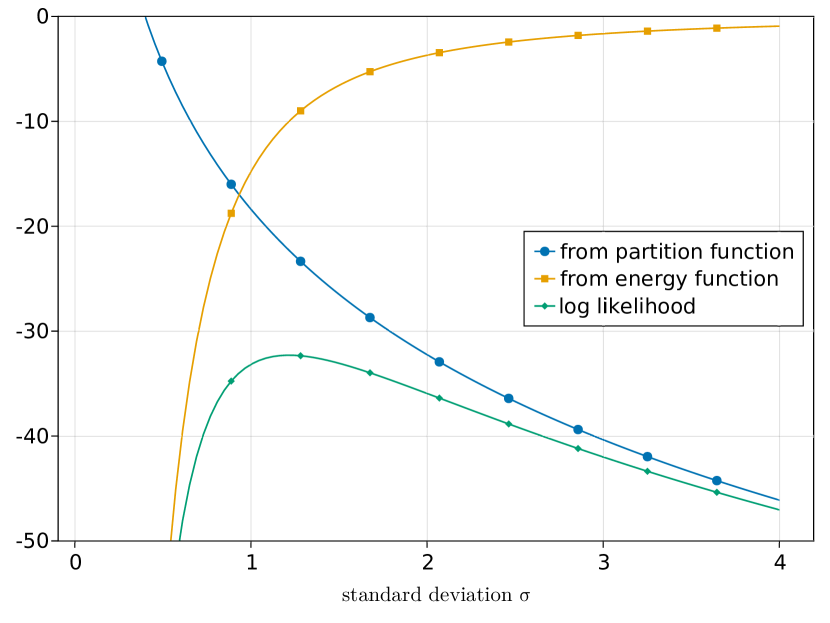
Figure 1: The log-likelihood function $\ell(\sigma)$ has two components that balance each other: the term due to the partition function monotonically decreases while the term due to the energy function monotonically increases. The balance between the two terms leads to a likelihood function $\ell(\sigma)$ with a well-defined optimum.

The contribution of the (log) partition function on the (log) likelihood function has two consequences: First, we cannot simply ignore the partition function if it is difficult to compute. In the simple Gaussian example in Figure 1, the maximum of the term due to the energy is achieved for $\sigma\to\infty$ irrespective of the data, which is not a meaningful estimator. Secondly, if we approximate the partition function, possible errors in the approximation may shift the location of the maximum, and hence affect the quality of the estimate.

2.3 Simulator-based model

Simulator-based models (SBMs) are another widely used class of models. They occur in multiple fields, for instance genetics (e.g. Beaumont et al., 2002; Marttinen et al., 2015), epidemiology (e.g. Allen, 2017; Parisi et al., 2021), systems biology (e.g. Wilkinson, 2018), cosmology (e.g. Schafer and Freeman, 2012) or econometrics (e.g. Gouriéroux and Monfort, 1996), just to name a few. Different research communities use different names so that SBMs are also known as e.g. implicit models (Diggle and Gratton, 1984) or stochastic simulation models (Hartig et al., 2011).

SBMs are specified via a measurable function $g$ that is typically not known in closed form but implemented as a computer programme. The function $g$ maps parameters $\boldsymbol{\theta}$ and realisations of some base random variable $\boldsymbol{\omega}$ to data $\mathbf{x}$, i.e.

$$\mathbf{x} =g(\boldsymbol{\omega},\boldsymbol{\theta}), \boldsymbol{\omega} \sim p(\boldsymbol{\omega}),$$ (17)

where $p(\boldsymbol{\omega})$ denotes the pdf of $\boldsymbol{\omega}$. Without loss of generality, we can assume that $\boldsymbol{\omega}$ are a collection of independent random variables uniformly distributed on the unit interval.

The distribution of $\mathbf{x}$ is defined by $g$ and the distribution of $\boldsymbol{\omega}$: The probability that $\mathbf{x}$ takes on some values in a set $\mathcal{A}$ is defined as

$$\Pr(\mathbf{x}\in\mathcal{A}|\boldsymbol{\theta})=\Pr(\{\omega:g(\boldsymbol{\omega},\boldsymbol{\theta})\in\mathcal{A}\}),$$ (18)

where the probability on the right-hand side is computed with respect to the distribution of $\boldsymbol{\omega}$. The randomness of $\boldsymbol{\omega}$ implies the randomness on the level of $\mathbf{x}$ and the function $g$ is thus said to “push forward” the distribution of $\boldsymbol{\omega}$ to $\mathbf{x}$. Determining the set of all $\boldsymbol{\omega}$ that are mapped to $\mathcal{A}$ for a given $\boldsymbol{\theta}$ corresponds to the problem of determining the inverse-image of $\mathcal{A}$ under $g$, see Figure 2.

Figure 2: The distribution of $\mathbf{x}$ in a simulator-based model is defined by the inverse-image of the intractable mapping $g(\boldsymbol{\omega},\boldsymbol{\theta})$ that maps base random variables $\boldsymbol{\omega}$ to data $\mathbf{x}$, and the inverse image changes when $\boldsymbol{\theta}$ is varied. The mapping $g$ is typically not known in closed form but implemented as a computer programme. This setup makes evaluating $p(\mathbf{x}|\boldsymbol{\theta})$ typically impossible.

Whilst the distribution of $\mathbf{x}$ is well defined for a given value of $\boldsymbol{\theta}$ (assuming that some technical measure-theoretical conditions on $g$ hold), writing down or computing the conditional pdf $p(\mathbf{x}|\boldsymbol{\theta})$ given the pdf $p(\boldsymbol{\omega})$ becomes quickly problematic when $g$ is not invertible. Moreover, in case of simulator-based models, we typically do not know a closed-form expression for $g$, which makes computing, or exactly evaluating, $p(\mathbf{x}|\boldsymbol{\theta})$ impossible.

The main advantage of SBMs is that they neatly connect the natural sciences with statistics and machine learning. We can use principled tools from statistics and machine learning to perform inference and experimental design for models from the natural sciences. The flip side, however, is that the likelihood function—the key workhorse for inference and experimental design—is typically intractable because the conditional pdf $p(\mathbf{x}|\boldsymbol{\theta})$ is intractable.

3 Contrastive learning

Contrastive learning is an alternative to likelihood-based learning when the model pdf and hence likelihood function is intractable. We first explain the basic idea and then discuss the two main ingredients of contrastive learning: the loss function and the choice of the contrast, or reference data.

3.1 Basic idea

The basic idea in contrastive learning is to learn the difference between the data of interest and some reference data. The properties of the reference are typically known or not of interest; by learning the difference we thus focus the (computational) resources on learning what matters.

Assuming that we are interested in a quantity $a$ and that our reference is $b$, we can deduce $a$ from $b$ when we know the difference between them:

$$\underbrace{b}_{\text{reference}}+\underbrace{a-b}_{\text{difference}}\Rightarrow\underbrace{a}_{\text{interest}}$$ (19)

This straightforward equation captures much of the essence of contrastive learning. This means that if we have some reference $b$ available, we can learn about $a$ by contrasting $a$ with $b$ rather than by starting from scratch.

There is an immediate link to (log) ratio estimation (e.g. Sugiyama et al., 2012a) when we let the quantity of interest and reference be $\log p_{a}$ and $\log p_{b}$, respectively,

$$\underbrace{\log p_{b}}_{\text{reference}}+\underbrace{\log p_{a}-\log p_{b}}_{\text{difference}}\Rightarrow\underbrace{\log p_{a}}_{\text{interest}}.$$ (20)

Here, contrasting $a$ with $b$ means learning the log-ratio $\log p_{a}-\log p_{b}$. This connects to logistic regression, and hence classification, which we will heavily exploit in this paper. The connection to classification makes intuitive sense since learning the difference between data sets is indeed what we need to do when solving a classification problem.

Denoting the log-ratio $\log p_{a}-\log p_{b}$ by $h$, let us write the above equation as

$$p_{a}=\exp(h)p_{b}.$$ (21)

We can thus express $p_{a}$ as a change of measure from $p_{b}$ where the learned log-ratio (difference) $h$ determines the change of measure.

There is also a direct connection to Bayesian inference because Bayes’ rule

$$p(\boldsymbol{\theta}|\mathbf{x})=\frac{p(\boldsymbol{\theta},\mathbf{x})}{p(\mathbf{x})}=\frac{p(\mathbf{x}|\boldsymbol{\theta})p(\boldsymbol{\theta})}{p(\mathbf{x})}$$ (22)

can be rewritten in the style of (20) as

$$\underbrace{\log p(\boldsymbol{\theta})}_{\text{reference}}+\underbrace{\log p(\mathbf{x}|\boldsymbol{\theta})-\log p(\mathbf{x})}_{\text{difference}}\Rightarrow\underbrace{\log p(\boldsymbol{\theta}|\mathbf{x})}_{\text{interest}},$$ (23)

with the log posterior as our quantity of interest $\log p_{b}$, the log prior as our reference $\log p_{a}$, and their difference (the “contrast”) proportional to the log likelihood. This reflects the role of the likelihood function in Bayesian inference as the quantity that transforms the prior belief into an unnormalised posterior belief.

3.2 Loss functions

In the following, we focus on the logistic, or log, loss as done in early work on contrastive learning to estimate energy-based models, i.e. noise-contrastive estimation (NCE, Gutmann and Hyvärinen, 2010, 2012). However, other loss functions can be used, e.g. Bregman divergences (Gutmann and Hirayama, 2011; Sugiyama et al., 2012b) or f-divergences (Nowozin et al., 2016), see also Mohamed and Lakshminarayanan (2017); Poole et al. (2019).

Given data of interest $\mathbf{x}_{o}=\{\mathbf{x}_{1},\ldots,\mathbf{x}_{n}\}$, with $\mathbf{x}_{i}\sim p$ (iid), and reference data $\{\mathbf{y}_{1},\ldots,\mathbf{y}_{m}\}$, $\mathbf{y}_{i}\sim q$ (iid), let us label the data points as follows. The $\mathbf{x}_{i}$ become tuples $(\mathbf{x}_{i},1)$ and the $\mathbf{y}_{i}$ become tuples $(\mathbf{y}_{i},0)$. Learning the difference between the $\mathbf{x}_{i}$ and $\mathbf{y}_{i}$ can then be cast as a problem of predicting the label for test points, which corresponds to classification.

A popular loss function for classification is the logistic loss, which means that we perform classification via (nonlinear) logistic regression. We denote this loss, normalised by the number of data points $n$, by $J(h)$,

$$J(h)= \frac{1}{n}\sum_{i=1}^{n}\log\left[1+\nu\exp(-h(\mathbf{x}_{i}))\right]+\frac{\nu}{m}\sum_{i=1}^{m}\log\left[1+\frac{1}{\nu}\exp(h(\mathbf{y}_{i}))\right],$$ (24)

where $\nu=m/n$ and the parameter of the loss is the function $h$. The minimal loss is achieved for a function $h$ that assigns large positive numbers to the $\mathbf{x}_{i}$ and large negative numbers to the $\mathbf{y}_{i}$. It can be shown (e.g. Gutmann and Hyvärinen, 2012; Thomas et al., 2020) that for large sample sizes $n$ and $m$ (and fixed ratio $\nu$), the optimal regression function $h$ equals

$$h^{\ast}=\log p-\log q.$$ (25)

This means that by solving the classification problem via logistic regression we learn the density ratio between $p$ and $q$. This important result reflects the connection between the different concepts discussed above, namely contrastive learning, classification via logistic regression, and density ratio estimation. The result implies consistency of the estimator for parametric models and finite amount of data under some technical conditions (e.g. Amemiya, 1985, Chapter 4).

Further important properties of the logistic loss are:

1. The optimal $h^{\ast}$ in (25) is “automagically” the difference between two log densities. This holds without us having to specify that $h$ should take this particular form. We will exploit this property in the estimation of unnormalised models, as well as in the Bayesian inference and experimental design for simulator-based models.

2. We only need samples from $p$ and $q$; we do not need their densities or models. This is important because we do not need to specify properly normalised pdfs as in likelihood-based learning and experimental design. However, we do need to model their ratio. This can be exploited as a modelling tool because it may often be easier to specify how the data of interest differs from the reference rather than specifying a parametric family of pdfs from scratch.

Both properties will be heavily exploited in the applications of contrastive learning to statistical inference and experimental design. Other loss functions mentioned above have the same properties.

When the sample sizes $n$ and $m$ are arbitrarily large, by the law of large numbers, the sample averages over $\mathbf{x}_{i}$ and $\mathbf{y}_{i}$ in (24) become expectations with respect to the densities $p$ and $q$, respectively. Denote the corresponding limiting loss function of $J(h)$ in (24) by $\bar{J}_{\nu}(h)$. Below, we will denote the limiting loss function in case of $\nu=1$ by $\bar{J}(h)$.

It is illustrative to consider the minimal loss $\bar{J}_{\nu}(h^{\ast})$ that is achieved by $h^{\ast}$,

$$\bar{J}_{\nu}(h^{\ast}) =\mathbb{E}_{\mathbf{x}\sim p}\log\left[1+\nu\frac{q(\mathbf{x})}{p(\mathbf{x})}\right]+\nu\mathbb{E}_{\mathbf{y}\sim q}\log\left[1+\frac{p(\mathbf{y})}{\nu q(\mathbf{y})}\right]$$ (26)

$$=\mathbb{E}_{\mathbf{x}\sim p}\log\left[\frac{p(\mathbf{x})+\nu q(\mathbf{x})}{p(\mathbf{x})}\right]+\nu\mathbb{E}_{\mathbf{y}\sim q}\log\left[\frac{\nu q(\mathbf{y})+p(\mathbf{y})}{\nu q(\mathbf{y})}\right]$$ (27)

$$=-\mathbb{E}_{\mathbf{x}\sim p}\log\left[\frac{p(\mathbf{x})}{p(\mathbf{x})+\nu q(\mathbf{x})}\right]-\nu\mathbb{E}_{\mathbf{y}\sim q}\log\left[\frac{\nu q(\mathbf{y})}{\nu q(\mathbf{y})+p(\mathbf{y})}\right].$$ (28)

Setting $\nu=1$ and introducing the mixture density $m=(p+q)/2$, we can write the above in terms of two Kullback-Leibler divergences, which furthermore can be expressed as the Jensen-Shannon divergence (JSD) between $p$ and $q$,

$$\bar{J}(h^{\ast}) \overset{\nu=1}{=}-\mathbb{E}_{\mathbf{x}\sim p}\log\left[\frac{p(\mathbf{x})}{p(\mathbf{x})+q(\mathbf{x})}\right]-\mathbb{E}_{\mathbf{y}\sim q}\log\left[\frac{q(\mathbf{y})}{q(\mathbf{y})+p(\mathbf{y})}\right]$$ (29)

$$=-\text{KL}(p||m)-\text{KL}(q||m)+2\log 2$$ (30)

$$=-\text{JSD}(p,q)+2\log 2.$$ (31)

Since $\bar{J}(h)\geq\bar{J}(h^{\ast})$, we have the following bound

$$\bar{J}(h)\geq-\text{JSD}(p,q)+2\log 2.$$ (32)

We can thus think that minimising $\bar{J}(h)$ with respect to $h$ leads to a variational estimate of the negative Jensen-Shannon divergence between $p$ and $q$ up to a known additive constant, which can be used to quantify the difference between $p$ and $q$ in the constructed classification problem.

3.3 Reference data

Much of the creative aspect of contrastive learning lies in the choice of the reference data. The choice depends on the application of contrastive learning, e.g. whether we are interested in model estimation or Bayesian inference. While intuition can partly guide the choice, establishing optimality results is an open research direction.

A simple option is to fit a preliminary model to the observed data $\mathbf{x}_{o}$ and to use data generated from the model as the reference. This has been done in the first work on estimating energy-based models with contrastive learning (noise-contrastive estimation, Gutmann and Hyvärinen, 2012). An extension is to iterate the above approach so that the fitted model in one iteration becomes the reference distribution in the next. Simulation results by Gutmann and Hyvärinen (2010) showed that this improved estimation accuracy compared to the “static” approach where the reference (noise) distribution was kept fixed. The reason for this is that at the start of a new iteration, the reference data includes all the information of the real data that was captured by the model so far, and a model-based classifier would not be able to distinguish between the reference data and the real data. The iteration forces the system to focus on the aspects of the real data that have not yet been captured by the model.

A further option is to create the reference data conditional on each observed data point so that each reference data point is paired with an observed data point. This is useful if the observed data lies on a lower-dimensional manifold for which fitting a preliminary model may be difficult (Ceylan and Gutmann, 2018).

In the iterative scheme above, each iteration essentially resets the classification performance to a 50% chance level. However, rather than periodically resetting the classification performance, one can also continuously update the reference distribution to push the classification performance towards chance level. This kind of iterative adaptive approach, which is known as “adversarial training”, has been used to estimate the parameters of a generative model specified by a neural network (generative adversarial networks, Goodfellow et al., 2014). The generative model can be seen to correspond to a simulator-based model where the function $g$ in (17) is given by a neural network and the parameters $\boldsymbol{\theta}$ that we would like to estimate are its weights. A similar adaptive scheme has been proposed by Gutmann et al. (2014, 2018) for both point and posterior estimation of general simulator-based models, see also the review by Mohamed and Lakshminarayanan (2017).

A complementary perspective is given by the variational bound in (32): learning the nonlinear regression function $h$ provides us with an estimate of the Jensen-Shannon divergence between the data distribution and the reference, and the adaptive updating of the reference distribution $q$ corresponds to a further optimisation that pushes the reference distribution $q$ towards the data distribution $p$ so that the Jensen-Shannon divergence between them is minimised.

Gao et al. (2020) used such an iterative adaptive scheme to learn an energy-based model choosing as reference distribution a normalising flow (see Papamakarios et al., 2021, for a comprehensive introduction to normalising flows). The normalising flow is continuously updated with the learning of the energy-based model to provide a strong reference distribution. As in case of the generative adversarial network above, the complementary perspective is that the flow is learned by (approximately) minimising the Jensen-Shannon to the data distribution. The benefit of this approach is twofold: On the one hand, the method enables the learning of an energy-based model in high-dimensions and is well suited for semi-supervised learning. On the other hand, the learned flow is by itself of interest since (a) it allows for exact sampling and (b) it is normalised and thus allows for likelihood evaluations.

When modelling time-series data, Hyvärinen and Morioka (2016) proposed to use windows of the time-series itself as the reference data. Under certain assumptions, this approach was shown to enable the estimation of independent components in a nonlinear time-series model (Hyvärinen and Morioka, 2016).

For Bayesian inference and experimental design, a natural choice of the reference data is to use the prior predictive distribution in line with the intuition in Section 3.1. This can be used to estimate the posterior distribution for simulator-based models and to perform experimental design as we will discuss below.

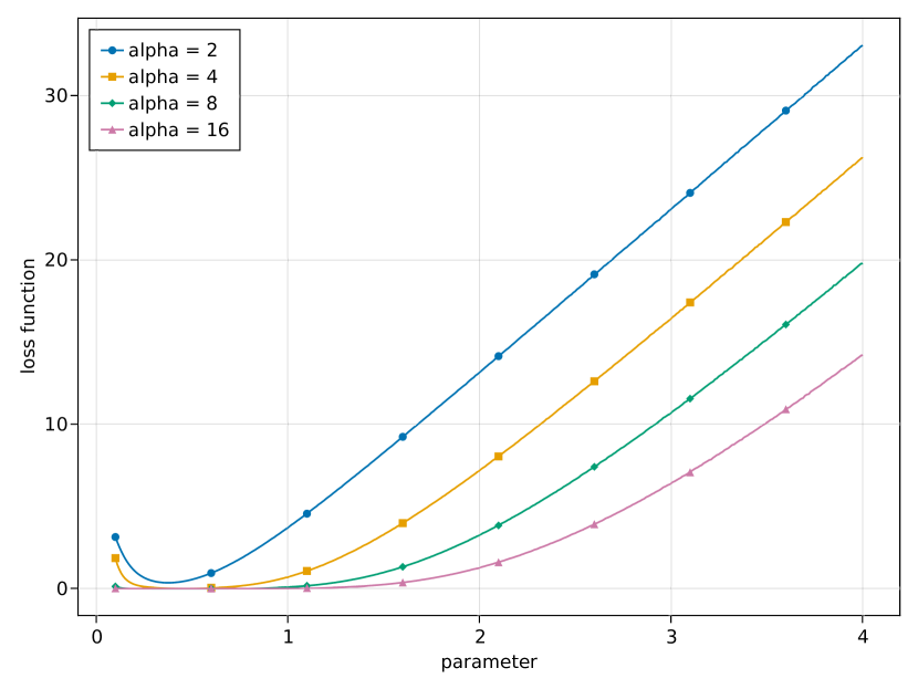
Figure 3: Logistic loss to learn the difference between a standard normal distribution and a Gaussian with standard deviation $\alpha$ in 10 dimensions. The log-ratio was parametrised by one free parameter acting on the squared norm of the random variables. The loss function becomes flatter around the optimum as $\alpha$ increases, i.e. as the two distributions become more different.

A major difficulty in contrastive learning with logistic regression is that learning the difference between the reference and data distribution accurately is difficult if they are very different. Intuitively, highly different distributions correspond to easy classification problems so that the classifier does not need to learn a lot about the structure of the data sets to achieve good performance. Another view is that several different classification boundaries can achieve similar performance, so that the loss function is flat around the optimum, which causes a larger estimation error. Figure 3 illustrates this behaviour in case of the logistic loss: the data follows a standard normal distribution and the reference is a Gaussian distribution with standard deviation $\alpha>1$ (in 10 dimensions). As $\alpha$ becomes larger, the reference distribution becomes more dissimilar from the data distribution and the loss function flatter around the optimum even though the scale of the loss function is about the same (and for large $\alpha$, the optimal parameter value equals 0.5 for all $\alpha$).

Rhodes et al. (2020) called this issues the “density chasm” problem and proposed a divide-and-conquer strategy to learn the ratio: Rather than attempting to learn the difference between $p_{a}$ and $p_{b}$ in one go, they introduce auxiliary distributions that anneal between $p_{a}$ and $p_{b}$. The auxiliary distributions are constructed so that the differences between them are sufficiently small so that their ratio can be better estimated, and the different estimates are then combined via a telescoping product (or sum in the log domain), i.e.

$$\underbrace{\log p_{a}-\log p_{b}}_{\text{large gap}}=\underbrace{\log p_{a}-\log p_{1}}_{\text{small gap}}+\sum_{k=1}^{K-1}\underbrace{(\log p_{k}-\log p_{k+1})}_{\text{small gap}}+\underbrace{\log p_{m}-\log p_{b}}_{\text{small gap}},$$ (33)

where the $p_{i}$ are the auxiliary densities. The functional form or a model of the auxiliary distributions does not need to be known since the method only requires samples from them. It is further possible to derive a limiting objective function when the number of auxiliary distributions $K$ goes to infinity, which was shown to lead to improved performance and removes the need to choose $K$ (Choi et al., 2021).

Telescoping density-ratio estimation by Rhodes et al. (2020); Choi et al. (2021) deals with the density chasm and the flat loss landscape by re-formulating the contrastive problem. A complementary algorithmic approach was taken by Liu et al. (2021) who asked whether optimisation techniques can deal with the flat optimisation landscape of the logistic loss when there is a density chasm. They found that, in case of exponential families, normalised gradient descent can deal with the issue. Moreover, they showed that a polynomial convergence guarantee can be obtained when working with the exponential rather than the logistic loss. The exponential loss is, like the logistic loss, a Bregman divergence that was shown to provide a large family of loss functions for the contrastive learning of energy-based models (Gutmann and Hirayama, 2011). The result by Liu et al. (2021) highlights that for some models, particular instances of the family of loss functions are more suitable than others.

4 Applications in statistical inference and experimental design

We here show how we can use contrastive learning to estimate energy-based models and perform Bayesian inference and experimental design for simulator-based models.

4.1 Estimating energy-based models

We introduced energy-based models (EBMs) in Section 2.2, pointing out that they are unnormalised models $\phi(\mathbf{x};\boldsymbol{\theta})=\exp(-E(\mathbf{x};\boldsymbol{\theta}))$ that are specified by an energy function $E(\mathbf{x};\boldsymbol{\theta})$. We have seen that standard maximum likelihood estimation cannot be used to learn the parameters $\boldsymbol{\theta}$ if the partition function $Z(\boldsymbol{\theta})$ in (10) is not available analytically in closed form.

Contrastive learning can be used to estimate energy-based models from data $\mathbf{x}_{o}=(\mathbf{x}_{1},\ldots,\mathbf{x}_{n})$, $\mathbf{x}_{i}\sim p$ (iid) by introducing reference data $(\mathbf{y}_{1},\ldots,\mathbf{y}_{m})$, $\mathbf{y}_{i}\sim q$ (iid) and estimating the log-ratio $h^{\ast}=\log p-\log q$. An estimate $\hat{h}$ thus provides an estimate of $p$ when $q$ is known,

$$\hat{p}=\exp(\hat{h})q,$$ (34)

where the factor $\exp(\hat{h})$ is a form of exponential tilting or a change of measure from $q$ to $p$ in line with (21).

There are different ways to parametrise $h$: If we would like to estimate an energy-based model where $\phi(\mathbf{x};\boldsymbol{\theta})$ has a specific form, we parametrise $h$ as

$$h(\mathbf{x};\boldsymbol{\theta},c)=\log\phi(\mathbf{x};\boldsymbol{\theta})-\log q(\mathbf{x})+c.$$ (35)

From (34), we can see that $q$ cancels out and hence

$$\hat{p}(\mathbf{x})=\exp(\hat{c})\phi(\mathbf{x};\hat{\boldsymbol{\theta}}).$$ (36)

The parameter $c$ allows for scaling of $\phi(\mathbf{x};\boldsymbol{\theta})$ and can optionally be included if $\phi(\mathbf{x};\boldsymbol{\theta})$ is not flexible enough. On the other hand, if we are not interested in estimating a specific model of a particular form, we may also parametrise $h$ directly, e.g. as a deep neural network in unsupervised deep learning.

This principle to learn energy-based models was proposed by Gutmann and Hyvärinen (2010, 2012) using the logistic loss. They called the reference distribution “noise” and the estimation principle hence “noise-contrastive-estimation”. The term “noise” should not be mis-understood to refer to unstructured data. As explained in Section 3, it can be structured and reflect our current understanding of the properties of the observed data $\mathbf{x}_{o}$. The above equations highlight two key conditions for the reference (noise) distribution $q$: (1) we need to be able to sample from it, (2) we need to know an analytical expression for it (strictly speaking, up to the normalisation constant only).

The fact that the model does not need to be normalised is due to property 1 of the logistic loss, namely that it yields the difference between two log densities, as in (25), without any normalisation constraints. Further loss functions with this property were proposed by Pihlaja et al. (2010); Gutmann and Hirayama (2011); Uehara et al. (2020). Moreover, the telescoping approach by Rhodes et al. (2020); Choi et al. (2021) can also be used to learn $h$, improving upon the single-ratio methods. For an overview of further methods to estimate energy-based models, we refer the reader to the recent review by Song and Kingma (2021), and for the case of energy-based models with latent (unobserved) variables to the work by Rhodes and Gutmann (2019).

In Section 3.3, we discussed an iterative approach where the estimated model from a previous iteration is used as reference (Gutmann and Hyvärinen, 2010). Goodfellow (2014) related this approach to maximum likelihood estimation. We here provide a simplified proof of the relationship. Let the log-ratio $h$ be parametrised by $\boldsymbol{\theta}$ and consider the loss function in (24) as function of $\boldsymbol{\theta}$,

$$J(\boldsymbol{\theta}) =\frac{1}{n}\sum_{i=1}^{n}\log\left[1+\nu\exp(-h(\mathbf{x}_{i};\boldsymbol{\theta}))\right]+\frac{\nu}{m}\sum_{i=1}^{m}\log\left[1+\frac{1}{\nu}\exp(h(\mathbf{y}_{i};\boldsymbol{\theta}))\right],$$ (37)

with $\mathbf{y}_{i}\sim q$ (iid) and $\nu=m/n$. The gradient with respect to $\boldsymbol{\theta}$ is

$$\nabla_{\boldsymbol{\theta}}J(\boldsymbol{\theta})= \frac{1}{n}\sum_{i=1}^{n}\frac{-\nu\exp(-h(\mathbf{x}_{i};\boldsymbol{\theta}))}{1+\nu\exp(-h(\mathbf{x}_{i};\boldsymbol{\theta}))}\nabla_{\boldsymbol{\theta}}h(\mathbf{x}_{i};\boldsymbol{\theta})+$$

$$\frac{1}{m}\sum_{i=1}^{m}\frac{\exp(h(\mathbf{y}_{i};\boldsymbol{\theta}))}{1+\frac{1}{\nu}\exp(h(\mathbf{y}_{i};\boldsymbol{\theta}))}\nabla_{\boldsymbol{\theta}}h(\mathbf{y}_{i};\boldsymbol{\theta}).$$ (38)

Assume now that the reference data $\mathbf{y}$ follows the distribution of the model at iteration $t$, i.e. $p(.;\boldsymbol{\theta}_{t})$. For a parametrisation of $h$ as in (35), we then have

$$h(\mathbf{x};\boldsymbol{\theta},c)=\log\phi(\mathbf{x};\boldsymbol{\theta})-\log p(\mathbf{x};\boldsymbol{\theta}_{t})+c$$ (39)

and the $\mathbf{y}_{i}\sim p(.;\boldsymbol{\theta}_{t})$. The gradient of $h(\mathbf{x};\boldsymbol{\theta},c)$ with respect to $\boldsymbol{\theta}$ is

$$\nabla_{\boldsymbol{\theta}}h(\mathbf{x};\boldsymbol{\theta},c)=\nabla_{\boldsymbol{\theta}}\log\phi(\mathbf{x};\boldsymbol{\theta})$$ (40)

and hence

$$\nabla_{\boldsymbol{\theta}}J(\boldsymbol{\theta})= \frac{1}{n}\sum_{i=1}^{n}\frac{-\nu\exp(-h(\mathbf{x}_{i};\boldsymbol{\theta}))}{1+\nu\exp(-h(\mathbf{x}_{i};\boldsymbol{\theta}))}\nabla_{\boldsymbol{\theta}}\log\phi(\mathbf{x}_{i};\boldsymbol{\theta})+$$

$$\frac{1}{m}\sum_{i=1}^{m}\frac{\exp(h(\mathbf{y}_{i};\boldsymbol{\theta}))}{1+\frac{1}{\nu}\exp(h(\mathbf{y}_{i};\boldsymbol{\theta}))}\nabla_{\boldsymbol{\theta}}\log\phi(\mathbf{y}_{i};\boldsymbol{\theta})$$ (41)

with $\mathbf{y}_{i}\sim p(.;\boldsymbol{\theta}_{t})$. Let us update $\boldsymbol{\theta}$ by gradient descent on $J(\boldsymbol{\theta})$ via

$$\boldsymbol{\theta}_{t+1}=\boldsymbol{\theta}_{t}-\epsilon\nabla_{\boldsymbol{\theta}}J(\boldsymbol{\theta})\big{|}_{\boldsymbol{\theta}=\boldsymbol{\theta}_{t}},$$ (42)

where $\epsilon$ is a small step-size. Note that in the evaluation of the gradient at $\boldsymbol{\theta}_{t}$, with (39), $h(\mathbf{x}_{i};\boldsymbol{\theta}_{t},c)=h(\mathbf{y}_{i};\boldsymbol{\theta}_{t},c)=c+\log Z(\boldsymbol{\theta}_{t})$, which is independent of $\mathbf{x}_{i}$ and $\mathbf{y}_{i}$. Let us denote its value by $b_{t}$. It measures the error in the normalisation of the unnormalised model: $b_{t}$ is close to zero if the parameter $c$ is close to the logarithm of the inverse partition function at $\boldsymbol{\theta}_{t}$, e.g. towards the end of the optimisation. Moreover, $b_{t}$ would be always zero in the special case of normalised models.

We thus obtain

$$\frac{-\nu\exp(-h(\mathbf{x}_{i};\boldsymbol{\theta}))}{1+\nu\exp(-h(\mathbf{x}_{i};\boldsymbol{\theta}))} =\frac{-\nu\exp(-b_{t})}{1+\nu\exp(-b_{t})}$$ (43)

$$\frac{\exp(h(\mathbf{y}_{i};\boldsymbol{\theta}))}{1+\frac{1}{\nu}\exp(h(\mathbf{y}_{i};\boldsymbol{\theta}))} =\frac{\nu}{1+\nu\exp(-b_{t})}$$ (44)

and hence

$$\nabla_{\boldsymbol{\theta}}J(\boldsymbol{\theta})\big{|}_{\boldsymbol{\theta}=\boldsymbol{\theta}_{t}}= \frac{-\nu}{1+\nu e^{-b_{t}}}\left(\frac{e^{-b_{t}}}{n}\sum_{i=1}^{n}\nabla_{\boldsymbol{\theta}}\log\phi(\mathbf{x}_{i};\boldsymbol{\theta})-\frac{1}{m}\sum_{i=1}^{m}\nabla_{\boldsymbol{\theta}}\log\phi(\mathbf{y}_{i};\boldsymbol{\theta})\right)\Big{|}_{\boldsymbol{\theta}=\boldsymbol{\theta}_{t}}$$ (45)

On the other hand, the gradient of the negative log-likelihood is

$$-\nabla_{\boldsymbol{\theta}}\ell(\boldsymbol{\theta})\big{|}_{\boldsymbol{\theta}=\boldsymbol{\theta}_{t}}= -\left(\frac{1}{n}\sum_{i=1}^{n}\nabla_{\boldsymbol{\theta}}\log\phi(\mathbf{x}_{i};\boldsymbol{\theta})-\mathbb{E}_{p(\mathbf{x};\boldsymbol{\theta}_{t})}\left[\nabla_{\boldsymbol{\theta}}\log\phi(\mathbf{x}_{i};\boldsymbol{\theta})\right]\right)\Big{|}_{\boldsymbol{\theta}=\boldsymbol{\theta}_{t}}$$ (46)

The average over the $\mathbf{y}_{i}\sim p(.;\boldsymbol{\theta}_{t})$ in (45) is a Monte Carlo estimate of the derivative of the log-partition function, which is the second term in (46). Hence for $b_{t}=0$, e.g. in case of normalised models, the gradient for contrastive learning with the logistic loss and $p(.;\boldsymbol{\theta}_{t})$ as reference distribution is a Monte Carlo approximation of the gradient of the negative log-likelihood (up to constant scaling factor that can be absorbed into the step-size). There is thus a clear connection between contrastive learning and maximum likelihood estimation: if, at every gradient step, we use the current model $p(.;\boldsymbol{\theta}_{t})$ as reference distribution, we follow noisy gradients of the (negative) log-likelihood.

This scheme, however, is typically computationally not feasible since sampling from $p(.;\boldsymbol{\theta}_{t})$ is prohibitively expensive. But we are not required to use at every iteration the current model. In contrastive learning, we are allowed to use the same “old” $p(.;\boldsymbol{\theta}_{t})$ to update the parameter $\boldsymbol{\theta}$ in the subsequent iterations. This results in a valid estimator (as in standard noise-contrastive estimation with a fixed reference distribution), but the gradient updates would not correspond to Monte Carlo approximations of the gradient of the negative log-likelihood.

A possibly simpler connection to maximum likelihood estimation can be obtained by considering the case of large $\nu$. Gutmann and Hyvärinen (2012) showed that for normalised models, noise-contrastive estimation is asymptotically equivalent to maximum likelihood estimation in the sense that the estimator has the same distribution irrespective of the choice of the reference distribution $q$ (as long as it satisfies some weak technical conditions). Moreover, Mnih and Kavukcuoglu (2013) showed that the gradient converges to the gradient of the negative log-likelihood. We can see this from (38) for $\nu\to\infty$: With $h(.;\boldsymbol{\theta})=\log\phi(.;\boldsymbol{\theta})-\log q(.)$, and

$$\lim_{\nu\to\infty}\frac{-\nu\exp(-h(\mathbf{x};\boldsymbol{\theta}))}{1+\nu\exp(-h(\mathbf{x};\boldsymbol{\theta}))} =-1$$ (47)

$$\lim_{\nu\to\infty}\frac{\exp(h(\mathbf{y};\boldsymbol{\theta}))}{1+\frac{1}{\nu}\exp(h(\mathbf{y};\boldsymbol{\theta}))} =\exp(h(\mathbf{y};\boldsymbol{\theta}))=\frac{\phi(\mathbf{y};\boldsymbol{\theta})}{q(\mathbf{y})},$$ (48)

taking the limit of $\nu\to\infty$ in (38) thus gives

$$\lim_{\nu\to\infty}\nabla_{\boldsymbol{\theta}}J(\boldsymbol{\theta})= -\frac{1}{n}\sum_{i=1}^{n}\nabla_{\boldsymbol{\theta}}\log\phi(\mathbf{x}_{i};\boldsymbol{\theta})+\mathbb{E}_{q(\mathbf{y})}\left[\frac{p(\mathbf{x};\boldsymbol{\theta})}{q(\mathbf{y})}\nabla_{\boldsymbol{\theta}}\log\phi(\mathbf{y};\boldsymbol{\theta})\right]$$ (49)

$$=-\frac{1}{n}\sum_{i=1}^{n}\nabla_{\boldsymbol{\theta}}\log\phi(\mathbf{x}_{i};\boldsymbol{\theta})+\mathbb{E}_{p(\mathbf{x};\boldsymbol{\theta})}\left[\nabla_{\boldsymbol{\theta}}\log\phi(\mathbf{y};\boldsymbol{\theta})\right],$$ (50)

where where have used that for $\nu\to\infty$, $m=\nu n$ becomes arbitrarily large too, so that the average over the $\mathbf{y}_{i}$ becomes an expectation with respect to $q(\mathbf{y})$. A more general result was established by Riou-Durand and Chopin (2018). Moreover, they further considered the case of finite $\nu$, but large sample sizes $n$, and showed that the variance of the noise-contrastive estimator is always smaller than the variance of the Monte Carlo MLE estimator (Geyer, 1994) where the partition function is approximated with a sample average, assuming in both cases that the auxiliary/reference distributions were fixed.

4.2 Bayesian inference for simulator-based models

Simulator-based models are specified by a stochastic simulator that is parametrised by a parameter $\boldsymbol{\theta}$. While we can generate (sample) data $\mathbf{x}$ by running the simulator, the conditional pdf $p(\mathbf{x}|\boldsymbol{\theta})$ of the generated data is typically not known in closed form, see Section 2.3. This makes standard likelihood-based learning of the parameters $\boldsymbol{\theta}$ impossible. The problem of estimating plausible values of $\boldsymbol{\theta}$ from some observed data $\mathbf{x}_{o}$ is called approximate Bayesian computation, likelihood-free inference, or simulator/simulation-based inference depending on the research community. For an introduction to the field, see the review papers by Lintusaari et al. (2017); Sisson et al. (2018); Cranmer et al. (2020).

We related contrastive learning to Bayes’ rule in Section 3.1. This connection is not merely conceptual but can be turned into an inference method to estimate the posterior pdf of the parameters $\boldsymbol{\theta}$ given observed data $\mathbf{x}_{o}$. Starting from Bayes’ rule in the log-domain,

$$\log p(\boldsymbol{\theta}|\mathbf{x})=\log p(\boldsymbol{\theta})+\log p(\mathbf{x}|\boldsymbol{\theta})-\log p(\mathbf{x})$$ (51)

we can estimate $p(\boldsymbol{\theta}|\mathbf{x})$ by learning the difference (log-ratio) $\log p(\mathbf{x}|\boldsymbol{\theta})-\log p(\mathbf{x})=\log p(\mathbf{x},\boldsymbol{\theta})-\log[p(\mathbf{x})p(\boldsymbol{\theta})]$ by contrastive learning and then combining it with the prior. To learn the difference, we can exploit that the model is specified in terms of a simulator that generates data from $p(\mathbf{x}|\boldsymbol{\theta})$, and hence also from the marginal (prior predictive) pdf $p(\mathbf{x})=\int p(\boldsymbol{\theta})p(\mathbf{x}|\boldsymbol{\theta})d\boldsymbol{\theta}$, which provides all the data that we need to learn the log-ratio. This approach to estimate the posterior was introduced by Thomas et al. (2016, 2020) and called “likelihood-free inference by ratio estimation”. An interesting property of this approach is that the learning of $h$ can be performed offline, prior to seeing the observed data $\mathbf{x}_{o}$, which enables amortisation of the inference.

The logistic loss in (24) is among the several loss functions that can be used for contrastive learning of the posterior. A simple approach is to minimise

$$J(h)= \frac{1}{n}\sum_{i=1}^{n}\log\left[1+\nu\exp(-h(\mathbf{x}_{i}))\right]+\frac{\nu}{m}\sum_{i=1}^{m}\log\left[1+\frac{1}{\nu}\exp(h(\mathbf{y}_{i}))\right]$$ (52)

with $\mathbf{x}_{i}\sim p(\mathbf{x}|\boldsymbol{\theta})$ (iid) and $\mathbf{y}_{i}\sim q$ (iid) with the contrastive distribution $q$ being equal to the marginal $p(\mathbf{x})$. Due to (25), the optimal $h$ is then indeed the desired $\log p(\mathbf{x}|\boldsymbol{\theta})-\log p(\mathbf{x})$ for any value of $\boldsymbol{\theta}$. Note that we are here again exploiting properties 1 and 2 of the logistic loss highlighted in Section 3.2.

Since the optimal $h$ is given by $\log p(\mathbf{x}|\boldsymbol{\theta})-\log p(\mathbf{x})$ for any $\boldsymbol{\theta}$, we can further amortise the inference with respect to $\boldsymbol{\theta}$ by averaging the loss function over different values of $\boldsymbol{\theta}$. When averaging over samples from the prior $p(\boldsymbol{\theta})$, this amounts to contrasting samples $(\mathbf{x},\boldsymbol{\theta})\sim p(\mathbf{x}|\boldsymbol{\theta})p(\boldsymbol{\theta})$ with samples $(\mathbf{x},\boldsymbol{\theta})\sim p(\mathbf{x})p(\boldsymbol{\theta})$, which was used by Hermans et al. (2020) together with MCMC to perform Bayesian inference.

In the approach described above, we contrasted simulated data with simulated data in order to essentially learn the intractable model pdf $p(\mathbf{x}|\boldsymbol{\theta})$. However, it is also possible to contrast the simulated data with the observed data to infer plausible values of $\boldsymbol{\theta}$ (Gutmann et al., 2014, 2018). For further information and connections to other work, including the learning of summary statistics, we refer the reader to (Pham et al., 2014; Thomas et al., 2016, 2020; Dinev and Gutmann, 2018; Hermans et al., 2020; Durkan et al., 2020; Chen et al., 2021).

4.3 Bayesian experimental design for simulator-based models

Let us now consider Bayesian experimental design for simulator-based models where the utility of an experiment is measured by the mutual information (MI) between the data and the quantity of interest (Chaloner and Verdinelli, 1995; Ryan et al., 2016). For simplicity, we here consider the situation where we are interested in the parameters $\boldsymbol{\theta}$ of a model. For other cases such as model discrimination, see e.g. (Ryan et al., 2016; Kleinegesse and Gutmann, 2021).

With (7), we thus would like to solve the following optimisation problem

$$\hat{\mathbf{d}} =\operatorname*{argmax}_{\mathbf{d}}\text{MI}_{\mathbf{d}}(\mathbf{x},\boldsymbol{\theta}), \text{MI}_{\mathbf{d}}(\mathbf{x},\boldsymbol{\theta}) =\mathbb{E}_{p(\mathbf{x},\boldsymbol{\theta}|\mathbf{d})}\log\left[\frac{p(\mathbf{x}|\boldsymbol{\theta},\mathbf{d})}{p(\mathbf{x}|\mathbf{d})}\right],$$ (53)

where $\mathbf{d}$ denotes the vector of design parameters. Since we are dealing with simulator-based models, the densities in the log-ratio are not available in closed form. This is the same issue as in case of Bayesian inference for simulator-based models considered above. But the problem is exacerbated by the following two further issues:

1. We need to know or evaluate the log ratio $\log p(\mathbf{x}|\boldsymbol{\theta},\mathbf{d})-\log p(\mathbf{x}|\mathbf{d})$ for (theoretically) infinitely many $\mathbf{x}$ due to the expected value in (53), and not only the observed data $\mathbf{x}_{o}$ as in Bayesian inference.

2. Furthermore, we not only need to evaluate the expected value of $\log p(\mathbf{x}|\boldsymbol{\theta},\mathbf{d})-\log p(\mathbf{x}|\mathbf{d})$ but also maximise it with respect to $\mathbf{d}$. This is typically done iteratively, which means that the log-ratios and expected values need to to re-estimated as $\mathbf{d}$ changes.

These issues make experimental design for simulator-based models by mutual information maximisation a highly difficult problem.

Kleinegesse and Gutmann (2019) proposed to build on the properties of the likelihood-free inference by ratio estimation framework (Thomas et al., 2016, 2020) to deal with the issues. As discussed in Section 4.2, the method yields an amortised log-ratio $\log p(\mathbf{x}|\boldsymbol{\theta},\mathbf{d})-\log p(\mathbf{x}|\mathbf{d})$ where, depending on the setup, the amortisation is with respect to $\mathbf{x}$ and $\boldsymbol{\theta}$, but not $\mathbf{d}$, which allowed them to estimate the expected value in (53) via a sample average over the learned log-ratios. This approach partly deals with the first issue above. For the optimisation (issue 2), Kleinegesse and Gutmann (2019) used Bayesian optimisation (e.g. Shahriari et al., 2016), which enables gradient-free optimisation and smoothes out Monte Carlo errors due to the sample average.

The work by Kleinegesse and Gutmann (2019) considered the static setting where prior to the experiment, we would determine the complete design. The methodology was extended to the sequential setting where we have the possibility to update our belief about $\boldsymbol{\theta}$ as we sequentially acquire the experimental data, see (Kleinegesse et al., 2021) for further information.

Learning the log ratios and accurately approximating the MI is computationally costly. However, we do not actually need to estimate the MI accurately everywhere. First, we are interested in the argument $\hat{\mathbf{d}}$ that maximises the MI rather than its value. Secondly, it is sufficient to be accurate around the optimum; cheaper but noisy or biased estimates of the MI and its gradient are sufficient during the search as long they lead us to $\hat{\mathbf{d}}$.

Such an approach was taken by Kleinegesse and Gutmann (2020, 2021) who concurrently tightened a variational lower bound on the mutual information (or proxy quantities) and maximised the (proxy) MI. Important related work is (Foster et al., 2019, 2020). This approach to experimental design for simulator-based models achieves large computational gains because we avoid approximating the mutual information accurately for values of $\mathbf{d}$ away from $\hat{\mathbf{d}}$. Kleinegesse and Gutmann (2021) showed that a large class off variational bounds are applicable and can be used for experimental design with various goal, e.g. parameter estimation or model discrimination.

Let us consider a special case of the framework that uses contrastive learning via the logistic loss and the bound in (32). Reordering the terms gives the following lower bound on the Jensen-Shannon divergence between the two densities $p$ and $q$,

$$\text{JSD}(p,q)\geq-\bar{J}(h)+2\log 2,$$ (54)

where $\bar{J}(h)$ is the logistic loss in (24) for $\nu=1$ and $n,m\to\infty$. Whilst the mutual information between data and parameters is defined in terms of the Kullback-Leibler (KL) divergence between the $p(\boldsymbol{\theta},\mathbf{x}|\mathbf{d})$ and $p(\boldsymbol{\theta}|\mathbf{d})p(\mathbf{x}|\mathbf{d})$, see (7), the Jensen-Shannon divergence has been found to be a practical alternative to the KL divergence due to its increased robustness (e.g. Hjelm et al., 2018).

Figure 4: Experimental design and posterior inference by maximising a lower bound on the Jensen-Shannon divergence (JSD) via the logistic loss. The example considers the design of measurement points in a stochastic SIR model in epidemiology. The quantities of interest are the infection rate and the recovery rate. Left top row: optimisation of the JSD lower bound. Left bottom row: learning trajectories of the optimal designs. Right: prior and estimated posterior for data acquired at the optimal design. The data was simulated with the ground-truth parameters indicated with a red cross. See Kleinegesse and Gutmann (2021) for details.

The lower bound in (54) allows us to perform experimental design for simulator-based models by letting $p(\boldsymbol{\theta},\mathbf{x}|\mathbf{d})$ and $p(\boldsymbol{\theta}|\mathbf{d})p(\mathbf{x}|\mathbf{d})$ play the role of $p$ and $q$, which means that $\bar{J}(h)$ becomes a function of $h$ and implicitly also of $\mathbf{d}$. Thus maximising $-\bar{J}(h)$, or minimising the logistic loss $\bar{J}(h)$, jointly with respect to $h$ and $\mathbf{d}$ allows us to concurrently tighten the bound and find the optimal design $\hat{\mathbf{d}}$. The optimisation of the logistic loss with respect to $h$ essentially corresponds to likelihood-free inference by ratio estimation that we discussed in Section 4.2. Thus, we here obtain not only the optimal design $\hat{\mathbf{d}}$ but also an amortised estimate of the posterior $p(\boldsymbol{\theta}|\mathbf{x},\hat{\mathbf{d}})$, see (Kleinegesse and Gutmann, 2020, 2021) for further details.

Figure 4 illustrates this approach for the design of experiments to estimate the parameters of a stochastic SIR model from epidemiology. The model has two parameters: the rate $\beta$ at which individuals are infected, and the rate $\gamma$ at which they recover. The model generates stochastic time-series of the number of infected and recovered people in a population and the design problem is to determine the times at which to measure these populations in order to best learn the parameters (see Kleinegesse and Gutmann (2021) for a detailed description of the setup). The top-left plot in Figure 4 shows the maximisation of the lower bound in (54) and the bottom-left plot shows the corresponding trajectories of the optimal designs. The sub-figure on the right shows the prior and estimated posterior for data acquired at the optimal design, i.e. the optimal measurement points.

If the simulator-based models are implemented such that automatic differentiation is supported, gradient-based optimisation is possible, which enables experimental design with higher dimensional design vectors $\mathbf{d}$. Furthermore, rather than optimising with respect to $\mathbf{d}$ directly, it is also possible to learn a policy which outputs the designs $\mathbf{d}$, which enables adaptive sequential design for simulator-based models (Ivanova et al., 2021).

5 Conclusions

The likelihood function is a main workhorse for statistical inference and experimental design. However, it is computationally intractable for several important classes of statistical models, including energy-based models and simulator-based models. This makes standard likelihood-based learning and experimental design impossible for those models. Contrastive learning offers an intuitive and computationally feasible alternative to likelihood-based learning. We have seen that contrastive learning is closely related to classification, logistic regression, and ratio estimation. By exploiting properties of the logistic loss, we have shown how contrastive learning can be used to solve a range of difficult statistical problems, namely (1) parameter estimation for energy-based models, (2) Bayesian inference for simulator-based models, and (3) Bayesian experimental design for simulator-based models. Whilst we focused on the logistic loss, we have pointed out that other loss functions can be used as well. The relative benefits and possible optimality properties of the different loss functions, as well as the reference data that is needed for contrastive learning, remain important open research questions.

Conflict of interest

The authors declare that they have no conflict of interest.

References

- Allen (2017) Allen LJS (2017) A primer on stochastic epidemic models: Formulation, numerical simulation, and analysis. Infectious Disease Modelling 2(2):128–142
- Amemiya (1985) Amemiya T (1985) Advanced Econometrics. Harvard University Press
- Aneja et al. (2021) Aneja J, Schwing A, Kautz J, Vahdat A (2021) A contrastive learning approach for training variational autoencoder priors. In: Beygelzimer A, Dauphin Y, Liang P, Vaughan JW (eds) Advances in Neural Information Processing Systems
- Beaumont et al. (2002) Beaumont MA, Zhang W, Balding DJ (2002) Approximate Bayesian Computation in Population Genetics. Genetics 162(4):2025–2035
- Ceylan and Gutmann (2018) Ceylan C, Gutmann MU (2018) Conditional noise-contrastive estimation of unnormalised models. In: Dy J, Krause A (eds) Proceedings of the 35th International Conference on Machine Learning (ICML), Proceedings of Machine Learning Research, vol 80, pp 725–733
- Chaloner and Verdinelli (1995) Chaloner K, Verdinelli I (1995) Bayesian Experimental Design: A Review. Statistical Science 10(3):273–304
- Chen et al. (2020) Chen T, Kornblith S, Norouzi M, Hinton G (2020) A simple framework for contrastive learning of visual representations. In: III HD, Singh A (eds) Proceedings of the 37th International Conference on Machine Learning, PMLR, Proceedings of Machine Learning Research, vol 119, pp 1597–1607
- Chen et al. (2021) Chen Y, Zhang D, Gutmann MU, Courville A, Zhu Z (2021) Neural approximate sufficient statistics for implicit models. In: International Conference on Learning Representations (ICLR)
- Choi et al. (2021) Choi K, Meng C, Song Y, Ermon S (2021) Density ratio estimation via infinitesimal classification. arXiv:211111010
- Cranmer et al. (2020) Cranmer K, Brehmer J, Louppe G (2020) The frontier of simulation-based inference. Proceedings of the National Academy of Sciences
- Diggle and Gratton (1984) Diggle PJ, Gratton RJ (1984) Monte Carlo methods of inference for implicit statistical models. Journal of the Royal Statistical Society Series B (Methodological) 46(2):193–227
- Dinev and Gutmann (2018) Dinev T, Gutmann M (2018) Dynamic likelihood-free inference via ratio estimation (DIRE). arXiv:181009899
- Du and Mordatch (2019) Du Y, Mordatch I (2019) Implicit generation and modeling with energy based models. In: Wallach H, Larochelle H, Beygelzimer A, d'Alché-Buc F, Fox E, Garnett R (eds) Advances in Neural Information Processing Systems, Curran Associates, Inc., vol 32
- Durkan et al. (2020) Durkan C, Murray I, Papamakarios G (2020) On contrastive learning for likelihood-free inference. In: Proceedings of the thirty-seventh International Conference on Machine Learning (ICML)
- Foster et al. (2019) Foster A, Jankowiak M, Bingham E, Horsfall P, Teh YW, Rainforth T, Goodman N (2019) Variational Bayesian optimal experimental design. In: Wallach H, Larochelle H, Beygelzimer A, d'Alché-Buc F, Fox E, Garnett R (eds) Advances in Neural Information Processing Systems, Curran Associates, Inc., vol 32
- Foster et al. (2020) Foster A, Jankowiak M, O’Meara M, Teh YW, Rainforth T (2020) A unified stochastic gradient approach to designing Bayesian-optimal experiments. In: Chiappa S, Calandra R (eds) Proceedings of the Twenty Third International Conference on Artificial Intelligence and Statistics, PMLR, Proceedings of Machine Learning Research, vol 108, pp 2959–2969
- Gao et al. (2020) Gao R, Nijkamp E, Kingma DP, Xu Z, Dai AM, Wu YN (2020) Flow contrastive estimation of energy-based models. In: Proceedings of the IEEE/CVF Conference on Computer Vision and Pattern Recognition (CVPR)
- Geyer (1994) Geyer CJ (1994) On the Convergence of Monte Carlo Maximum Likelihood Calculations. Journal of the Royal Statistical Society Series B (Methodological) 56(1):261–274
- Goodfellow et al. (2014) Goodfellow I, Pouget-Abadie J, Mirza M, Xu B, Warde-Farley D, Ozair S, Courville A, Bengio Y (2014) Generative adversarial nets. In: Ghahramani Z, Welling M, Cortes C, Lawrence ND, Weinberger KQ (eds) Advances in Neural Information Processing Systems 27, Curran Associates, Inc., pp 2672–2680
- Goodfellow (2014) Goodfellow IJ (2014) On distinguishability criteria for estimating generative models. arXiv:14126515
- Gouriéroux and Monfort (1996) Gouriéroux C, Monfort A (1996) Simulation-Based Econometric Methods (Core Lectures). Oxford University Press
- Grathwohl et al. (2021) Grathwohl W, Swersky K, Hashemi M, Duvenaud D, Maddison CJ (2021) Oops i took a gradient: Scalable sampling for discrete distributions. In: Proceedings of the 38th International Conference on Machine Learning (ICML), PMLR, 139, pp 3831–3841
- Green et al. (2015) Green P, Latuszynski K, Pereyra M, Robert CP (2015) Bayesian computation: a summary of the current state, and samples backwards and forwards. Statistics and Computing 25(4):835–862
- Gutmann and Hyvärinen (2009) Gutmann M, Hyvärinen A (2009) Learning features by contrasting natural images with noise. In: Proceedings of the International Conference on Artificial Neural Networks (ICANN), Springer Berlin Heidelberg, pp 623–632
- Gutmann and Hirayama (2011) Gutmann MU, Hirayama J (2011) Bregman divergence as general framework to estimate unnormalized statistical models. In: Proceedings of the Conference on Uncertainty in Artificial Intelligence (UAI)
- Gutmann and Hyvärinen (2010) Gutmann MU, Hyvärinen A (2010) Noise-contrastive estimation: A new estimation principle for unnormalized statistical models. In: Teh YW, Titterington M (eds) Proceedings of the International Conference on Artificial Intelligence and Statistics (AISTATS), JMLR Workshop and Conference Proceedings, Chia Laguna Resort, Sardinia, Italy, Proceedings of Machine Learning Research, vol 9, pp 297–304
- Gutmann and Hyvärinen (2012) Gutmann MU, Hyvärinen A (2012) Noise-contrastive estimation of unnormalized statistical models, with applications to natural image statistics. Journal of Machine Learning Research 13:307–361
- Gutmann and Hyvärinen (2013) Gutmann MU, Hyvärinen A (2013) A three-layer model of natural image statistics. Journal of Physiology-Paris 107(5):369–398
- Gutmann et al. (2014) Gutmann MU, Dutta R, Kaski S, Corander J (2014) Likelihood-free inference via classification. arXiv:14074981
- Gutmann et al. (2018) Gutmann MU, Dutta R, Kaski S, Corander J (2018) Likelihood-free inference via classification. Statistics and Computing 28(2):411–425
- Hartig et al. (2011) Hartig F, Calabrese JM, Reineking B, Wiegand T, Huth A (2011) Statistical inference for stochastic simulation models – theory and application. Ecology Letters 14(8):816–827
- Hermans et al. (2020) Hermans J, Begy V, Louppe G (2020) Likelihood-free MCMC with amortized approximate ratio estimators. In: Proceedings of the thirty-seventh International Conference on Machine Learning (ICML)
- Hjelm et al. (2018) Hjelm RD, Fedorov A, Lavoie-Marchildon S, Grewal K, Bachman P, Trischler A, Bengio Y (2018) Learning deep representations by mutual information estimation and maximization. In: International Conference on Learning Representations
- Hyvärinen and Morioka (2016) Hyvärinen A, Morioka H (2016) Unsupervised feature extraction by time-contrastive learning and nonlinear ica. In: Lee D, Sugiyama M, Luxburg U, Guyon I, Garnett R (eds) Advances in Neural Information Processing Systems, Curran Associates, Inc., vol 29
- Ivanova et al. (2021) Ivanova DR, Foster A, Kleinegesse S, Gutmann MU, Rainforth T (2021) Implicit deep adaptive design: Policy-based experimental design without likelihoods. In: Proceedings of the Thirty-fifth Conference on Neural Information Processing Systems (NeuRIPS 2021), Neural Information Processing Systems