Failed Disruption Propagation in Integer Genetic Programming

Abstract.

We inject a random value into the evaluation of highly evolved deep integer GP trees 9 743 720 times and find 99.7% of test outputs are unchanged. Suggesting crossover and mutation’s impact are dissipated and seldom propagate outside the program. Indeed only errors near the root node have impact and disruption falls exponentially with depth at between $e^{-{\rm depth}/3}$ and $e^{-{\rm depth}/5}$ for recursive Fibonacci GP trees, allowing five to seven levels of nesting between the runtime perturbation and an optimal test oracle for it to detect most errors. Information theory explains this locally flat fitness landscape is due to FDP. Overflow is not important and instead, integer GP, like deep symbolic regression floating point GP and software in general, is not fragile, is robust, is not chaotic and suffers little from Lorenz’ butterfly.

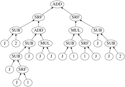
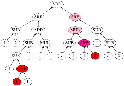
Figure 1. Left: an evolved Fibonacci solution. The arrows show the information flow from the leafs to the root node (top oval). The root gives the output of the whole program. Right: Evaluation of the tree showing two examples of run time disruption. 1) When the bottom most J node (in red) is artificially perturbed by +1, the disruption only reaches the calling SRF function (in red), whose output does not change. 2) Similarly, on most test cases, disrupting the other red J node by +1, means its calling SRF node’s (dark pink) output does not change. On test case J=0, the disruption propagates 3 levels to the pink SRF node. On test case J=1, the disruption propagates as far as the pink MUL node. (See page 1.1 and Sections 3.3 and 3.7.)

4 page version to appear in GECCO ’22 Companion, July 9–13, 2022 ACM ISBN 978-1-4503-9268-6/22/07.
https://doi.org/10.1145/3520304.3528878

1. Information Theory

We can view computing as processing information (Renyi, 1987). Information in the program’s inputs is transformed as it passes through the program and emerges at its outputs. In deterministic programs, there is no information gain. Indeed only in the special case that the program is reversible (Langdon, 2003, 2009) is the amount of information (number of Shannon bits) in the output the same as that which went into the program. In real programs, the information content is reduced. That is computing destroys information.

Further individual operations inside a digital computer may destroy information. Excluding the special case of reversible functions, all the functions from which a program is made individually loose information. For example, a 32 bit addition operation takes two inputs and creates one output. The inputs may each contain up to 32 bits of information (total 64 bits) but its output can contain no more than 32 bits of information. Storing data in memory allows the program to retain information, but when that data is used, its information is liable to be reduced or even lost (Clark et al., 2020). Computation maps multiple input patterns to the same output. For example: 3 + 5 and 2 + 6, each give the same value, 8. If we follow the input data’s path through an executing program, e.g. we trace 3,5 in one run and 2,6 in another, where the paths meet, e.g. at + giving 8, there is potential entropy (Renyi, 1987) loss. Note, from the value 8 we cannot tell if we started with 3,5 or 2,6.

Much of genetic programming is concerned with evolving functions without side effects. For example in symbolic regression GP evolves trees which take data from (32 bit) floating point inputs and generates a (32 bit) floating point output at its root node. The information compression is even more dramatic in GP binary classification problems where all the information in the tree’s inputs is reduced to at most a single bit.

We can view GP primitives as information funnels (Langdon et al., 2021b), with wide mouths which take information from the function’s inputs and a narrower output, corresponding to less information leaving the function. In tree GP it is easy to see the whole tree as being made from information funnels, with one funnel per node in the tree, see Figure 2. We can view crossover, mutation, and even runtime glitches, as injecting a disruption into the GP tree.

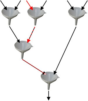
Figure 2. Each information funnel represents an irreversible function taking in total more information than leaves it. (Output at bottom.) Disruption (in red) is progressively dissipated and may not change the output at all.

If a deep GP tree is perturbed, the disruption has to propagate from the crossover point, mutation or error, up the tree through many levels to the root node before it has any impact on the tree’s fitness. It is known in conventional programming (Androutsopoulos et al., 2014; Petke et al., 2021) that often disruptions fail to propagate. We argue that this stems directly from information loss and so is inherent in all computation, including GP. We have shown that failed disruption propagation (FDP) can be common in deep floating point expressions (Langdon et al., 2022). The mechanisms which cause FDP can vary between programs. For example in GP symbolic regression, FDP is often associated with rounding errors (Langdon et al., 2022). To show an example which is independent of floating point rounding, we will show (in Section 3) that failed disruption propagation also occurs in deep integer GP trees, where calculations are performed exactly. We find small (+1) and large (RANDINT, Section 3.7) run time disruptions rapidly dissipate in similar ways. Section 2 describes the integer Fibonacci Problem we will use and Section 4 discusses our results and their implications for GP and software more widely.

1.1. Disrupting Integer Arithmetic

Much of Koza’s first GP book (Koza, 1992) is concerned with either floating point or Boolean expressions. However Koza also introduces the problem of inducing an integer tree which recursively generates the Fibonacci sequence of positive integers. Therefore we shall use the Fibonacci Problem and demonstrate in deep GP trees failed disruption propagation can also be common in exact arithmetic.

We use GP to evolve large GP trees by simply running to 1000 generations rather than stopping at the first solution. We then re-evaluate the whole tree on all the training cases having first inserted a fixed run time perturbation at a given location. We step though every location in this large highly evolved fit tree and keep a record of which perturbations do or do not cause a change in evaluation at the root node and on which test case.

Like Danglot et al. (Danglot et al., 2018), the first perturbation is simply to add 1 to the evaluation (on each test case) at the chosen point in the tree. This can be thought of as the minimum perturbation. We also repeat the experiment but instead of making a small change we simply totally replace the original evaluation by a randomly chosen 32 bit signed integer value.

2. Koza’s Fibonacci Benchmark

The Fibonacci sequence 1, 1, 2, 3, 5, 8… is an infinite sequence of positive integers, where the next one is given by summing the two previous items in the list. For training we take the first 20 members of the sequence, i.e. from the 0^th (1) to the 19^th (6765). See Table 1. The primitives Koza (Koza, 1992) uses are the four small integers 0, 1, 2 and 3, the sequence index J, the three integer arithmetic operations: addition, subtraction and multiplication. In addition, to support recursion, there is a special function SRF which also takes two arguments. SRF allows access to values calculated by the GP tree on earlier test cases. SRF’s first argument is the number of the test case. SRF’s second argument is a default value, to be used if the first argument is invalid. (For simplicity all arguments, including where we have multiplication by zero, are always evaluated.) As an example (SRF 1 0) will evaluate to 0 on the first two (J=0 and J=1) test cases, and will evaluate to the evolved individual’s answer for test case J=1 on later tests. Test cases are always run in order, starting at J=0. Notice, in Section 3, where tree evaluations are deliberately disrupted, the disruption is applied per test case and therefore SRF can access the earlier unchanged tree evaluations.

Table 1. GP to create deep fit Fibonacci trees for
Failed Disruption Propagation (FDP) experiments

Terminal set:	J, 0, 1, 2, 3
Function set:	ADD SUB MUL SRF
Fitness cases:	First 20 members of the Fibonacci sequence.
Selection:	Fitness = $\sum_{\rm J=0}^{19}|{\rm GP(J)}-{\rm Fibonacci\,}_{\rm J}|$.   I.e. the sum of the absolute error between GP’s answer and the value of the Jth member of the Fibonacci sequence. Tournament size 7.
Population:	Panmictic, non-elitist, generational.
GP parameters:	Initial population of 50 000 trees created by ramped half and half (Koza, 1992) with depth between 2 and 6. 100% unbiased subtree crossover. 1000 generations. No size or depth limit.

2.1. Background

Perhaps because, by early GP standards, the Fibonacci Problem needs a large population, see Figure 3, it has been little used in GP. However 17 years after Koza’s book was published, At EuroGP 2009 Harding et al. gave a nice summary (Harding et al., 2009). Their survey includes (Huelsbergen, 1997), (Nishiguchi and Fujimoto, 1998), (Agapitos and Lucas, 2006), (Shirakawa et al., 2007), and (Wilson and Heywood, 2007), all of these used approaches to the Fibonacci Problem which differ from Koza’s (Koza, 1992). Except Kouchakpour (Kouchakpour, 2008), publications on inducing the Fibonacci sequence since EuroGP 2009 have all looked at non-standard GP. They include Castle’s 2012 PhD thesis (Castle, 2012) which used it as one of half a dozen benchmarks to compare Montana’s strongly typed GP (Montana, 1995) with Castle’s own Strongly Formed GP and with other higher level imperative primitive sets. Also in 2012 Bryson and Ofria (Bryson and Ofria, 2012) used Avida to evolve solutions. Whilst Atkinson’s 2019 PhD thesis (Atkinson, 2019) looked at solution by evolving graphs. In 2018 Krauss et al. (Krauss et al., 2018) used it with a very different AST representation in their genetic improvement (Langdon, 2012; Petke et al., 2019) experiments.

Other work includes: Gruau et al. (Gruau et al., 1995) who used a Fibonacci program as an example to show coding Pascal programs as neural networks. Teller’s 1998 PhD thesis (Teller, 1998) which includes it as a simple example of neural programming. Yu who showed that programs generating the Fibonacci sequence can be evolved using higher-order functions (Yu, 2005). It has also been used to demonstrate Spector’s Push (Spector et al., 2005) and by Binard (Binard and Felty, 2007) to demonstrate System F. Finally Kouchakpour’s 2008 PhD thesis returned to Koza’s setting of the Fibonacci Problem (Kouchakpour, 2008).

3. Experiments

3.1. Tuning for Tournament Selection

We did a series of tuning GP runs to choose the population size (Table 1). From Figure 3 we can see that the chance of success with tournament size 7, separate, non-overlapping, generations (i.e. with complete replacement) and a population of 2000 trees is only 1.3%. So we chose a population of 50 000, where about 47% of runs find programs which pass all 20 Fibonacci fitness tests by generation 50.

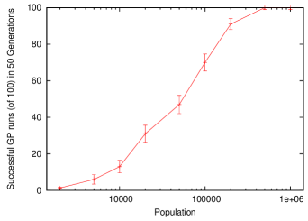
Figure 3. Number of successful Fibonacci runs.

3.2. Ten Extended Runs to 1000 Generations

In order to get deep fit Fibonacci trees to try our disruption experiments on, we ran our GP with a population of 50 000 for 1000 generations. (We used the same parameters, Table 1.) Of course without size or depth limits, the GP bloats (Langdon and Poli, 1997) (see Figures 4 to 8). At the end of each run a Fibonacci tree was selected for perturbation. The runs are summarised in Table 3.2. (Column 3 gives the expected depth for a random binary tree of a given size, column 1, whilst column 4 gives the standard deviation (Flajolet and Oldyzko, 1982).)

To reduce run time we used our (Langdon, 2021c) incremental and “fitness first” (Langdon, 2021a) evaluation. Of course this does not effect the course of evolution but reduces the number of opcodes evaluated by between 27 and 41 fold. (See Figure 7. Figure 9 gives the absolute speed in terms of GP operations/second, GPops (Langdon and Harrison, 2008).)

Figure 4. Mean size of trees in ten extended GP Fibonacci runs (population 50 000). Note log scale.

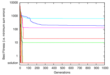
Figure 5. Sum of training $|$error$|$ in ten extended GP Fibonacci runs (population 50 000). Note log scale.

Figure 6. Mean fraction of children with fitness different from their first (i.e. root donating) parent in ten extended GP Fibonacci runs (population 50 000). Note log scale.

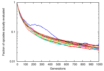
Figure 7. Effectiveness of incremental evaluation at exploiting FDP and convergence to reduce the volume of GP opcodes that must be evaluated to calculate fitness. (Ten extended GP Fibonacci runs with population 50 000). By generation 1000, only 2.9% of opcodes are evaluated. Note log scale.

Figure 8. Mean number of functions evaluated above crossover point per test case in ten extended GP Fibonacci runs using incremental evaluation (Langdon, 2021c) (population 50 000). Note linear scale.

Table 2. Ten Deep Fit GP Fibonacci Trees

Size	Depth		Fitness		Output disruption on any test
		(Langdon, 2000)	sum $|$error$|$		+1		RANDINT
86035	663	735 (	160 )	20	0.114 %	-0.31	0.092 %	-0.31
4347	160	165 (	36 )	10	1.449 %	-0.30	1.449 %	-0.33
23289	220	383 (	83 )	184	3.010 %	-0.27	3.053 %	-0.27
131159	449	908 (	197 )	130	0.127 %	-0.28	0.121 %	-0.29
77479	454	698 (	152 )	632	0.253 %	-0.20	0.256 %	-0.20
51697	626	570 (	124 )	0	0.056 %	-0.27	0.056 %	-0.27
771	33	64 (	14 )	0	7.523 %	-0.21	7.523 %	-0.22
35727	425	474 (	103 )	0	0.073 %	-0.30	0.073 %	-0.30
53305	485	579 (	126 )	0	0.032 %	-0.33	0.032 %	-0.33
23377	360	383 (	83 )	0	0.137 %	-0.26	0.137 %

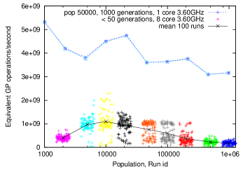
Figure 9. GP speed. Lower: 100 runs for each population size. (For visualisation small x-direction noise added.) Top: in ten 1000 generations runs GP tends to converge (Langdon, 2022b) making the speed up of incremental evaluation (Langdon, 2021c) more effective. Note top (single core) data are spread out horizontally for visualisation only.

3.3. Fraction of +1 Disruptive Perturbations

In almost all locations in the ten deep highly evolved GP Fibonacci trees, the +1 disruption at run time fails to reach the root node on all twenty training cases. The right hand side of Table 3.2 gives the fraction (%, column 6) which disrupt fitness on any of the twenty test cases. Even for the three shallowest trees more than 90% of the perturbations fail to propagate to the program’s output on any test case. Therefore the fitness would be identical despite the runtime change. In most cases the fraction of FDP on any of the fitness cases is well in excess of 99% (max 99.968% for run 9).

In floating point symbolic regression (Langdon et al., 2022) failed disruption propagation depends on the magnitude of the test case (with values near zero being suppressed most easily). In contrast, Figure 11 shows in the Fibonacci Problem almost the same behaviour for all test cases. This suggests Fibonacci test cases are not independent. Which in turn hints at potential runtime saving by sub-sampling test cases. Only the zeroth test case (J=0) is slightly different, and we see disruption dying away even faster than in the other nineteen test cases. Notice in Figure 11, FDP behaves similarly across ten very different trees. Each shows, for each test case, a similar exponential decrease in the number of functions the +1 disruption propagates through before becoming totally lost. Column 7 in Table 3.2 gives the exponent for the decrease with depth averaged (median) across all twenty test cases. The values lies between -0.33 and -0.20, meaning on average between 14 and 23 nested functions will reduce disruption by 100 fold.

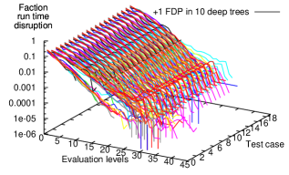
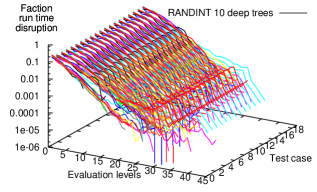
Figure 10. How far +1 disruption travels up tree for each training case (0–19). Small fraction which reach the root node on any test are given in Table 3.2 and not plotted here. Table 3.2 also gives median slope of these plots. Note log scale.

Figure 11. How far RANDINT disruption travels up tree for each training case (0–19). Small fraction which reach the root node on any test are given in Table 3.2 and not plotted here. Table 3.2 also gives median slope. Note log scale.

3.4. Location of +1 Disruptive Perturbations

The small fraction of +1 disruptions which reach the root node, on any test case, and so do change fitness, lie close to the root node itself. I.e, the disruption travels only a short distance through the code. Depending on run, most lie within 4–9 levels of the root node. For most runs (see Figure 13) more than 99% of these disrupted evaluations start within 8 nested function calls of the root. Runs 1, 3 and 5 have long tails, so that more than 1% of disrupted evaluations start more than 20 levels deep. Even so in these runs no disruption traverses more than 31 levels and still impacts fitness.

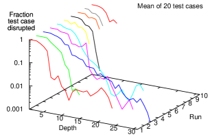
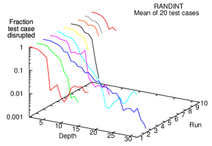
Figure 12. Location of +1 disruptions which affect fitness on any training case. (See also left side of Figures 14 and 15.) Note log scale.

Figure 13. Location of RANDINT disruptions which affect fitness on any training case. (See also right side of Figures 14 and 15.) Note log scale.

3.5. Integer Overflow

In the +1 FDP experiments, except for one subtraction, only integer multiplication leads to overflowing 32 bits. The fraction of multiplication (MUL) node outputs being truncated to 32 bits varies considerably between runs. In most cases there is none or very little ($<$1%), in others between 5% and 23% of disrupted multiplications overflow. In all cases, +1 disruption which causes 32 bit integer overflow is stopped by the usual mechanisms (see next section) and does not reach the program’s output.

3.6. Fibonacci Mechanisms for Failed Disruption Propagation

Although we argue that information theory suggests that failed disruption propagation is universal, we can see specific mechanisms for FDP in the Fibonacci Problem. For simplicity let us just consider cases where the disruption on all 20 test cases stops at the same point. 20% of such +1 disruptions stop on a multiply by zero. That is, one argument of multiply is zero and so disruption to the other fails to propagate past the multiply, since its output is zero regardless of the disruption. All the others stop on a SRF function. Of these most (98.7%) are because the SRF node returned its default value as it did before the disruption. This may be because the SRF function’s first argument (the index) was already invalid and so caused SRF to return its default value (the 2^nd argument). And if disrupting the index value still leaves it invalid, the SRF will continue to return its unchanged default value. Meaning the disruption stops at the SRF node.

3.7. RANDINT Disruption

We repeated the above experiments replacing the small perturbation, which simply added one to the evaluation of each point in each large GP tree for each test case, by replacing the existing evaluation by a random integer value. The value was chosen uniformly at random from all $2^{32}$ possible signed integer values. Then as before we trace how far the large disruption propagates through the evolved tree.

Starting with Table 3.2 we see that the large RANDINT disruption behaves very similarly to the +1 disruption. Comparing the last four columns of Table 3.2, we see almost all large disruptions fail to reach the root node and so make no difference to the program’s output or fitness. And further the exponential rate (between $-1/3$ and $-1/5$) with which the average disruption dies away with distance from the root node, although different between runs, is very similar for +1 and RANDINT. Comparing Figures 11 and 11 again shows little difference between the distance traveled through the evolved code by the large and small disruptions. Whilst Figures 13 and 13 show the small fraction of large and small disruptions which are able to reach the program’s output are similarly clustered close to the output itself (the root node). Figures 14 and 15, next section, also show that +1 and RANDINT have similar patterns of failed disruption propagation.

When disrupting by replacing an evaluation by a large value (rather than making a small change), both addition and subtraction may subsequently overflow 32 bits. However multiplication continues to be by far the most likely operation to cause overflow. Again there is variation between runs with between 30% and 65% of disruptions leading to overflow. Of the small fraction of RANDINT disruptions which reach the root (column 8 in Table 3.2), between 1% and 38% are affected by overflow.

3.8. Disruptable code lies near the output

Figures 14 and 15 compare the impact of the +1 and random replacement perturbations. (To reduce clutter, SRF functions are shown with =.) The plots are each in five rows of horizontal pairs. In each row the same program is shown. With the impact of increasing each evaluation by +1 shown on the left and the impact of replacement with a random 32 bit value (RANDINT) on the right. The plots show the binary trees using Daida’s circular lattice (Daida et al., 2005). This can be thought of as viewing the binary tree from the top looking down on the root node (in the center) with each side subtree spread out around it. The colours indicate how many times the program’s answer is changed when evaluation at that point in the program is disrupted on each test case.

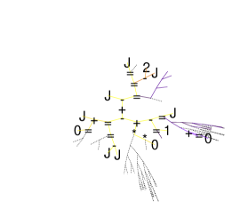
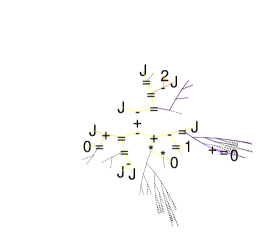
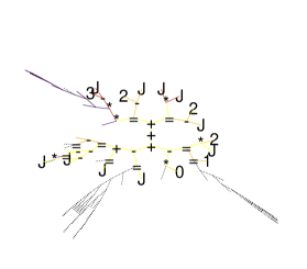
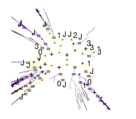
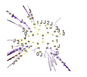
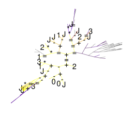
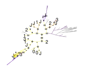
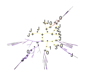
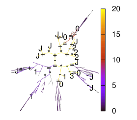
Figure 14. Colour shows location of run time disruption in evolved tree and number of test cases (1–20) where it impacts the tree’s output. GP trees plotted with output at center of circular lattice (Daida et al., 2005). Almost all the trees are grey meaning no impact but only center -10:+10 shown. = indicates SRF node, * multiplication. Runs 1–5. Left +1, right RANDINT.

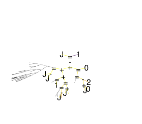
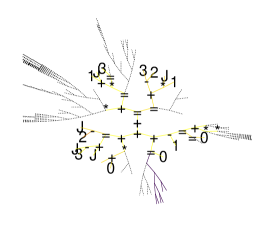
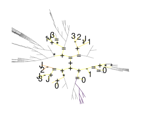
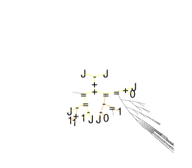
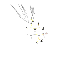
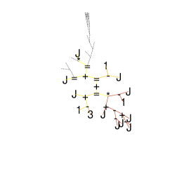
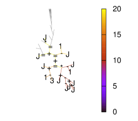
Figure 15. Colour shows location of run time disruption in evolved tree and number of test cases (1–20) where it impacts the tree’s output. GP trees plotted with output at center of circular lattice (Daida et al., 2005). Almost all the trees are grey meaning no impact but only center -10:+10 shown. = indicates SRF node, * multiplication. Runs 6–10. Left +1, right RANDINT.

As expected, the root node (center) is always disrupted and so is shown in bright yellow (20 test cases). The number of test cases disrupted falls monotonically with distance from the root node. Dotted gray lines indicates parts of the tree where disruption does not reach the root node on any test case. For ease of comparison, each plot is shown at the same scale with parts of the tree outside the square box (-10:$+$10)² centered on the root node not being plotted. In half the runs, this box captures all the parts of the tree where disruption does reach the root node. Indeed in all runs all the heavily disrupted parts (bright yellow) are plotted. Only in the third run, is there code which is disruptive on more than three cases (blue) which is not plotted because it lies outside -10:$+$10.

4. Discussion

At first sight it seems surprising in a continuous domain (albeit with exact arithmetic) that arguably the smallest (+1) and largest (RANDINT) disruptions should behave almost identically. However the two problem dependent mechanisms for failed disruption propagation (identified in Section 3.6) apply to both small and large changes. That is 1) multiplication by zero, gives a zero result, no matter how small or large the other argument is and 2) SRF will return its default value if its first argument is just out of range or if it is widely out of range.

With the small disruption and 32 bit arithmetic, integer overflow seldom occurs and if it does, it makes no difference to failed disruption propagation. With the large change, overflow is more common but it still make little difference to FDP.

We have used various recent efficiency improvements to Singleton’s GPquick (Langdon, 2020, 2021b, 2021a). In particular with extended runs (Langdon and Banzhaf, 2022) incremental evaluation (Langdon, 2021c) again gave substantial speed up without affecting evolution.

Columns 3 and 4 of Table 3.2 show again (Langdon et al., 1999), but now over an extensive period (1000 generations rather than (Langdon et al., 1999)’s 50 or 75), with two arity functions and no size or depth constraints (Table 1) that GP evolves trees whose shape is similar to that of most binary trees (Flajolet and Oldyzko, 1982).

We see highly evolved integer GP programs, like floating point (Langdon et al., 2021a) and human written code (Langdon and Petke, 2015) (Brownlee et al., 2020), are not fragile. Indeed they are robust not only to genetic changes like crossover, but to run time errors, which they did not encounter during training.

4.1. Lorenz’ butterfly need not trouble software

Edward N. Lorenz (1972) was uncertain if a single flap of a butterfly’s wings in one hemisphere could cause a dramatic change in the weather the other side of the equator but argued that the atmosphere is chaotic and so difficult to predict in the short term (Lorenz, 1993).

We have argued that deterministic programs are not chaotic. We have shown often a single perturbation deep within such software has no effect. Whereas the atmosphere’s chaos is powered by all the Sun’s energy falling on the Earth and contains an unmeasurable number of flapping wings, deterministic programs (in particular GP) dissipate information and so (mostly) give the same result even if a “butterfly” or other “bug” flips some bits deep within them (Danglot et al., 2018).

4.2. Good and bad failed disruption propagation

The impact of failed disruption propagation is profound. It is a two edged sword. One side means crossovers, mutations, perturbations, radiation, coding errors, etc., may only have local impact and their disruption may monotonically fall to nothing. Making the software robust. The other edge cuts the tester: Even if an error, glitch or bug infects the local state (Voas, 1992), if it is far from the tester’s software or hardware probe the disruption may have faded away before it can be recorded. Thus rendering the test ineffective and leaving the error undetected. However although undetected now, possibly it may have an effect on a customer later.

4.3. Better Evolutionary Computation?

In tree GP (Koza, 1992), almost all crossovers or mutations occur near leafs far from the root node. In deep trees, their impact is often lost before it reaches the program’s output (the root node). In artificial systems we are free to choose where to place mutations and where to cut and slice in recombination. So we could opt to place such disruption close to the root node. However, if we are to evolve complex programs with many many features, they will have to be large.

Evolving a monolithic one or two dimensional structure with all information channeled via a single output node risks the program being so deep that it is impossible to measure the fitness of most genetic updates, or, if we move the crossover locations to be by the output node, we have the problem of carrying a large dead weight of code which cannot adapt beneath a tiny living evolving surface near the route node. Therefore instead we may want to adopt a porous open sponge like high dimensional structure, with a large surface area, where much of the program (and hence most of the genetic locations) is close to the program’s environment (Langdon, 2022a).

5. Conclusions

We have measured software engineering’s failed disruption propagation (FDP) (Petke et al., 2021) in genetic programming and find as predicted by information theory in integer functions it is very common. On average in our deep trees 99.7% of large run time disruptions fail to propagate to the root node and so have no impact on fitness.

We see failed disruption propagation scaling at between $e^{-{\rm depth}/3}$ and $e^{-{\rm depth}/5}$, meaning the chance of detecting disruption (be it induced by crossover, mutation, cosmic ray or indeed software bug) falls significantly within 3 to 5 levels. Indeed, with every extra level of nesting the effectiveness of optimal test oracle placement or fitness measurement falls by between 18% and 28%.

We see little difference between the smallest possible disruption (Section 3.3) and total runtime randomization (Section 3.7), suggesting Danglot et al.’s (Danglot et al., 2018) correctness attraction will hold more widely than their +1 disruption. Indeed these experiments with integer functions, support the view that software is not fragile (Langdon and Petke, 2015).

The average depth, rather than size, is critical. With nesting deeper than 5–7 levels it becomes impossible to see the effect of most individual crossovers or mutations and the fitness landscape becomes increasingly flat and evolution harder. This suggests either the need to limit the depth of crossover and mutation or the need to move fitness testing from the root node to closer to the genetic changes (Langdon, 2022a).

Acknowledgments

This work was inspired by conversations at Dagstuhl Seminar 18052 on Genetic Improvement of Software (Petke et al., 2018). I am grateful for the assistance of anonymous reviewers. Supported by the Meta OOPS project.

GPQuick code is available in http://www.cs.ucl.ac.uk/staff/W.Langdon/ftp/gp-code/GPinc.tar.gz

References

- (1)
- Agapitos and Lucas (2006) Alexandros Agapitos and Simon M. Lucas. 2006. Learning Recursive Functions with Object Oriented Genetic Programming. In Proceedings of the 9th European Conference on Genetic Programming (Lecture Notes in Computer Science, Vol. 3905), Pierre Collet, Marco Tomassini, Marc Ebner, Steven Gustafson, and Anikó Ekárt (Eds.). Springer, Budapest, Hungary, 166–177. http://dx.doi.org/10.1007/11729976_15
- Androutsopoulos et al. (2014) Kelly Androutsopoulos, David Clark, Haitao Dan, Robert M. Hierons, and Mark Harman. 2014. An Analysis of the Relationship between Conditional Entropy and Failed Error Propagation in Software Testing. In International Conference on Software Engineering (ICSE 2014), Lionel Briand and Andre van der Hoek (Eds.). ACM, Hyderabad, India, 573–583. http://dx.doi.org/10.1145/2568225.2568314
- Atkinson (2019) Timothy Atkinson. 2019. Evolving Graphs by Graph Programming. Ph.D. Dissertation. University of York, UK. https://ethos.bl.uk/OrderDetails.do?uin=uk.bl.ethos.803685
- Binard and Felty (2007) Franck Binard and Amy Felty. 2007. An abstraction-based genetic programming system. In Late breaking paper at Genetic and Evolutionary Computation Conference (GECCO’2007), Peter A. N. Bosman (Ed.). ACM Press, London, United Kingdom, 2415–2422. http://dx.doi.org/10.1145/1274000.1274004
- Brownlee et al. (2020) Alexander Brownlee, Justyna Petke, and Anna F. Rasburn. 2020. Injecting Shortcuts for Faster Running Java Code. In 2020 IEEE Congress on Evolutionary Computation (CEC), Alexander (Sandy) Brownlee, Saemundur O. Haraldsson, Justyna Petke, and John R. Woodward (Eds.). IEEE, Internet. http://dx.doi.org/10.1109/CEC48606.2020.9185708 Special Session on Genetic Improvement.
- Bryson and Ofria (2012) David M. Bryson and Charles Ofria. 2012. Digital Evolution Exhibits Surprising Robustness to Poor Design Decisions. In ALIFE 2012: The Thirteenth International Conference on the Synthesis and Simulation of Living Systems. MIT, East Lansing, Michigan, USA, 19–26. http://dx.doi.org/10.1162/978-0-262-31050-5-ch003
- Castle (2012) Thomas Anthony Castle. 2012. Evolving High-Level Imperative Program Trees with Genetic Programming. PhD Thesis. University of Kent, UK. http://kar.kent.ac.uk/34799/
- Clark et al. (2020) David Clark, W. B. Langdon, and Justyna Petke. 2020. Software Robustness: A Survey, a Theory, and Some Prospects. Presented at Facebook Testing and Verification Symposium 2020. https://fbresearchevents.bevylabs.com/events/details/facebook-tav-symposium-division-facebook-testing-and-verification-symposium-presents-dress-rehearsal-facebook-tav-symposium-2020/
- Daida et al. (2005) Jason M. Daida, Adam M. Hilss, David J. Ward, and Stephen L. Long. 2005. Visualizing Tree Structures in Genetic Programming. Genetic Programming and Evolvable Machines 6, 1 (March 2005), 79–110. http://dx.doi.org/10.1007/s10710-005-7621-2
- Danglot et al. (2018) Benjamin Danglot, Philippe Preux, Benoit Baudry, and Martin Monperrus. 2018. Correctness attraction: a study of stability of software behavior under runtime perturbation. Empirical Software Engineering 23, 4 (1 Aug. 2018), 2086–2119. http://dx.doi.org/10.1007/s10664-017-9571-8
- Flajolet and Oldyzko (1982) Philippe Flajolet and Andrew Oldyzko. 1982. The Average Height of Binary Trees and Other Simple Trees. J. Comput. System Sci. 25, 2 (October 1982), 171–213. https://doi.org/10.1016/0022-0000(82)90004-6
- Gruau et al. (1995) Frederic Gruau, Jean-Yves Ratajszczak, and Gilles Wiber. 1995. A Neural Compiler. Theoretical Computer Science 141, 1 (17 April 1995), 1–52. http://dx.doi.org/10.1016/0304-3975(94)00200-3
- Harding et al. (2009) Simon Harding, Julian Miller, and Wolfgang Banzhaf. 2009. Self Modifying Cartesian Genetic Programming: Fibonacci, Squares, Regression and Summing. In Proceedings of the 12th European Conference on Genetic Programming, EuroGP 2009 (LNCS, Vol. 5481), Leonardo Vanneschi, Steven Gustafson, Alberto Moraglio, Ivanoe De Falco, and Marc Ebner (Eds.). Springer, Tuebingen, 133–144. http://dx.doi.org/10.1007/978-3-642-01181-8_12
- Huelsbergen (1997) Lorenz Huelsbergen. 1997. Learning Recursive Sequences via Evolution of Machine-Language Programs. In Genetic Programming 1997: Proceedings of the Second Annual Conference, John R. Koza, Kalyanmoy Deb, Marco Dorigo, David B. Fogel, Max Garzon, Hitoshi Iba, and Rick L. Riolo (Eds.). Morgan Kaufmann, Stanford University, CA, USA, 186–194. http://bell-labs.co/who/lorenz/papers/gp97.pdf
- Ibarra-Vazquez et al. (2021) Gerardo Ibarra-Vazquez, Gustavo Olague, Cesar Puente, Mariana Chan-Ley, and Carlos Soubervielle-Montalvo. 2021. Automated Design of Accurate and Robust Image Classifiers with Brain Programming. In Proceedings of the Genetic and Evolutionary Computation Conference Companion (Lille, France) (GECCO ’21). Association for Computing Machinery, New York, NY, USA, 1385–1393. http://dx.doi.org/10.1145/3449726.3463179
- Kouchakpour (2008) Peyman Kouchakpour. 2008. Population Variation in Canonical Tree-based Genetic Programming. Ph.D. Dissertation. School of Electrical, Electronic and Computer Engineering, University of Western Australia, Perth, Australia. http://robotics.ee.uwa.edu.au/theses/2008-Genetic-Kouchakpour-PhD.pdf
- Koza (1992) John R. Koza. 1992. Genetic Programming: On the Programming of Computers by Means of Natural Selection. MIT Press, Cambridge, MA, USA. http://mitpress.mit.edu/books/genetic-programming
- Krauss et al. (2018) Oliver Krauss, Hanspeter Moessenboeck, and Michael Affenzeller. 2018. Dynamic Fitness Functions for Genetic Improvement in Compilers and Interpreters. In 5th edition of GI @ GECCO 2018, Brad Alexander, Saemundur O. Haraldsson, Markus Wagner, John R. Woodward, and Shin Yoo (Eds.). ACM, Kyoto, Japan, 1590–1597. http://dx.doi.org/10.1145/3205651.3208308
- Langdon (2000) W. B. Langdon. 2000. Quadratic Bloat in Genetic Programming. In Proceedings of the Genetic and Evolutionary Computation Conference (GECCO-2000), Darrell Whitley, David Goldberg, Erick Cantu-Paz, Lee Spector, Ian Parmee, and Hans-Georg Beyer (Eds.). Morgan Kaufmann, Las Vegas, Nevada, USA, 451–458. http://gpbib.cs.ucl.ac.uk/gecco2000/GA069.pdf
- Langdon (2003) W. B. Langdon. 2003. The distribution of Reversible Functions is Normal. In Genetic Programming Theory and Practice, Rick L. Riolo and Bill Worzel (Eds.). Kluwer, Chapter 11, 173–187. http://dx.doi.org/10.1007/978-1-4419-8983-3_11
- Langdon (2009) W. B. Langdon. 2009. Scaling of Program Functionality. Genetic Programming and Evolvable Machines 10, 1 (March 2009), 5–36. http://dx.doi.org/10.1007/s10710-008-9065-y
- Langdon (2012) W. B. Langdon. 2012. Genetic Improvement of Programs. In 18th International Conference on Soft Computing, MENDEL 2012 (2nd ed.), Radomil Matousek (Ed.). Brno University of Technology, Brno, Czech Republic. http://www.cs.ucl.ac.uk/staff/W.Langdon/ftp/papers/Langdon_2012_mendel.pdf Invited keynote.
- Langdon (2020) W. B. Langdon. 2020. Multi-threaded Memory Efficient Crossover in C++ for Generational Genetic Programming. SIGEVOLution newsletter of the ACM Special Interest Group on Genetic and Evolutionary Computation 13, 3 (Oct. 2020), 2–4. http://dx.doi.org/10.1145/3430913.3430914
- Langdon (2021a) William B. Langdon. 2021a. Fitness First. In Genetic Programming Theory and Practice XVIII (Genetic and Evolutionary Computation), Wolfgang Banzhaf, Leonardo Trujillo, Stephan Winkler, and Bill Worzel (Eds.). Springer, East Lansing, MI, USA, 143–164. http://dx.doi.org/10.1007/978-981-16-8113-4_8
- Langdon (2021b) William B. Langdon. 2021b. Fitness First and Fatherless Crossover. In Proceedings of the Genetic and Evolutionary Computation Conference Companion (GECCO ’21), Francisco Chicano, Alberto Tonda, Krzysztof Krawiec, Marde Helbig, Christopher W. Cleghorn, Dennis G. Wilson, Georgios Yannakakis, Luis Paquete, Gabriela Ochoa, Jaume Bacardit, Christian Gagne, Sanaz Mostaghim, Laetitia Jourdan, Oliver Schuetze, Petr Posik, Carlos Segura, Renato Tinos, Carlos Cotta, Malcolm Heywood, Mengjie Zhang, Leonardo Trujillo, Risto Miikkulainen, Bing Xue, Aneta Neumann, Richard Allmendinger, Fuyuki Ishikawa, Inmaculada Medina-Bulo, Frank Neumann, and Andrew M. Sutton (Eds.). Association for Computing Machinery, Internet, 253–254. http://dx.doi.org/10.1145/3449726.3459437
- Langdon (2021c) William B. Langdon. 2021c. Incremental Evaluation in Genetic Programming. In EuroGP 2021: Proceedings of the 24th European Conference on Genetic Programming (LNCS, Vol. 12691), Ting Hu, Nuno Lourenco, and Eric Medvet (Eds.). Springer Verlag, Virtual Event, 229–246. http://dx.doi.org/10.1007/978-3-030-72812-0_15
- Langdon (2022a) W. B. Langdon. 2022a. Evolving Open Complexity. SIGEVOlution newsletter of the ACM Special Interest Group on Genetic and Evolutionary Computation 15, 1 (March 2022). http://arxiv.org/abs/2112.00812
- Langdon (2022b) W. B. Langdon. 2022b. Genetic Programming Convergence. Genetic Programming and Evolvable Machines 23, 1 (March 2022), 71–104. http://dx.doi.org/10.1007/s10710-021-09405-9
- Langdon et al. (2022) William B. Langdon, Afnan Alsubaihin, and David Clark. 2022. Measuring Failed Disruption Propagation in Genetic Programming. In Proceedings of the 2022 Genetic and Evolutionary Computation Conference (GECCO ’22), Alma Rahat, Jonathan Fieldsend, Markus Wagner, Sara Tari, Nelishia Pillay, Irene Moser, Aldeida Aleti, Ales Zamuda, Ahmed Kheiri, Erik Hemberg, Christopher Cleghorn, Chao li Sun, Georgios Yannakakis, Nicolas Bredeche, Gabriela Ochoa, Bilel Derbel, Gisele L. Pappa, Sebastian Risi, Laetitia Jourdan, Hiroyuki Sato, Petr Posik, Ofer Shir, Renato Tinos, John Woodward, Malcolm Heywood, Elizabeth Wanner, Leonardo Trujillo, Domagoj Jakobovic, Risto Miikkulainen, Bing Xue, Aneta Neumann, Richard Allmendinger, Inmaculada Medina-Bulo, Slim Bechikh, Andrew M. Sutton, and Pietro Simone Oliveto (Eds.). Association for Computing Machinery, Boston, USA.
- Langdon and Banzhaf (2022) William B. Langdon and Wolfgang Banzhaf. 2022. Long-Term Evolution Experiment with Genetic Programming. Artificial Life 28, 2 (2022). http://www.cs.ucl.ac.uk/staff/W.Langdon/ftp/papers/Langdon_2022_ALJ.pdf Invited submission to Artificial Life Journal special issue of the ALIFE’19 conference.
- Langdon and Harrison (2008) W. B. Langdon and A. P. Harrison. 2008. GP on SPMD parallel Graphics Hardware for mega Bioinformatics Data Mining. Soft Computing 12, 12 (Oct. 2008), 1169–1183. http://dx.doi.org/10.1007/s00500-008-0296-x Special Issue on Distributed Bioinspired Algorithms.
- Langdon and Petke (2015) William B. Langdon and Justyna Petke. 2015. Software is Not Fragile. In Complex Systems Digital Campus E-conference, CS-DC’15 (Proceedings in Complexity), Pierre Parrend, Paul Bourgine, and Pierre Collet (Eds.). Springer, 203–211. http://dx.doi.org/10.1007/978-3-319-45901-1_24 Invited talk.
- Langdon et al. (2021a) William B. Langdon, Justyna Petke, and David Clark. 2021a. Dissipative Polynomials. In 5th Workshop on Landscape-Aware Heuristic Search (GECCO 2021 Companion), Nadarajen Veerapen, Katherine Malan, Arnaud Liefooghe, Sebastien Verel, and Gabriela Ochoa (Eds.). ACM, Internet, 1683–1691. http://dx.doi.org/10.1145/3449726.3463147
- Langdon et al. (2021b) William B. Langdon, Justyna Petke, and David Clark. 2021b. Information Loss Leads to Robustness. IEEE Software Blog. http://blog.ieeesoftware.org/2021/09/information-loss-leads-to-robustness-w.html
- Langdon and Poli (1997) W. B. Langdon and R. Poli. 1997. Fitness Causes Bloat. In Soft Computing in Engineering Design and Manufacturing, P. K. Chawdhry, R. Roy, and R. K. Pant (Eds.). Springer-Verlag London, 13–22. http://dx.doi.org/10.1007/978-1-4471-0427-8_2
- Langdon et al. (1999) William B. Langdon, Terry Soule, Riccardo Poli, and James A. Foster. 1999. The Evolution of Size and Shape. In Advances in Genetic Programming 3, Lee Spector, William B. Langdon, Una-May O’Reilly, and Peter J. Angeline (Eds.). MIT Press, Cambridge, MA, USA, Chapter 8, 163–190. http://www.cs.ucl.ac.uk/staff/W.Langdon/aigp3/ch08.pdf
- Lorenz (1993) Edward N. Lorenz. 1993. The Butterfly Effect. In The Essence of Chaos. University of Washington Press, Seattle, USA, Chapter Appendix 1, 181–184. https://uwapress.uw.edu/book/9780295975146/the-essence-of-chaos/
- Montana (1995) David J. Montana. 1995. Strongly Typed Genetic Programming. Evolutionary Computation 3, 2 (Summer 1995), 199–230. http://dx.doi.org/10.1162/evco.1995.3.2.199
- Nishiguchi and Fujimoto (1998) Masato Nishiguchi and Yoshiji Fujimoto. 1998. Evolutions of Recursive Programs with Multi-Niche Genetic Programming (mnGP). In Proceedings of the 1998 IEEE World Congress on Computational Intelligence. IEEE Press, Anchorage, Alaska, USA, 247–252. http://dx.doi.org/10.1109/ICEC.1998.699720
- Petke et al. (2019) Justyna Petke, Brad Alexander, Earl T. Barr, Alexander E. I. Brownlee, Markus Wagner, and David R. White. 2019. A Survey of Genetic Improvement Search Spaces. In 7th edition of GI @ GECCO 2019, Brad Alexander, Saemundur O. Haraldsson, Markus Wagner, and John R. Woodward (Eds.). ACM, Prague, Czech Republic, 1715–1721. http://dx.doi.org/10.1145/3319619.3326870
- Petke et al. (2021) Justyna Petke, David Clark, and William B. Langdon. 2021. Software Robustness: A Survey, a Theory, and Some Prospects. In ESEC/FSE 2021, Ideas, Visions and Reflections, Paris Avgeriou and Dongmei Zhang (Eds.). ACM, Athens, Greece, 1475–1478. http://dx.doi.org/10.1145/3468264.3473133
- Petke et al. (2018) Justyna Petke, Claire Le Goues, Stephanie Forrest, and William B. Langdon. 2018. Genetic Improvement of Software: Report from Dagstuhl Seminar 18052. Dagstuhl Reports 8, 1 (23 July 2018), 158–182. http://dx.doi.org/10.4230/DagRep.8.1.158
- Renyi (1987) Alfred Renyi. 1987. A Diary on Information Theory. John Wiley and Sons, Chichester.
- Shirakawa et al. (2007) Shinichi Shirakawa, Shintaro Ogino, and Tomoharu Nagao. 2007. Graph structured program evolution. In GECCO ’07, Dirk Thierens, Hans-Georg Beyer, Josh Bongard, Jurgen Branke, John Andrew Clark, Dave Cliff, Clare Bates Congdon, Kalyanmoy Deb, Benjamin Doerr, Tim Kovacs, Sanjeev Kumar, Julian F. Miller, Jason Moore, Frank Neumann, Martin Pelikan, Riccardo Poli, Kumara Sastry, Kenneth Owen Stanley, Thomas Stutzle, Richard A Watson, and Ingo Wegener (Eds.), Vol. 2. ACM Press, London, 1686–1693. http://dx.doi.org/10.1145/1276958.1277290
- Spector et al. (2005) Lee Spector, Jon Klein, and Maarten Keijzer. 2005. The Push3 execution stack and the evolution of control. In GECCO 2005, Hans-Georg Beyer, Una-May O’Reilly, Dirk V. Arnold, Wolfgang Banzhaf, Christian Blum, Eric W. Bonabeau, Erick Cantu-Paz, Dipankar Dasgupta, Kalyanmoy Deb, James A. Foster, Edwin D. de Jong, Hod Lipson, Xavier Llora, Spiros Mancoridis, Martin Pelikan, Guenther R. Raidl, Terence Soule, Andy M. Tyrrell, Jean-Paul Watson, and Eckart Zitzler (Eds.), Vol. 2. ACM Press, Washington DC, USA, 1689–1696. http://dx.doi.org/10.1145/1068009.1068292
- Teller (1998) Astro Teller. 1998. Algorithm Evolution with Internal Reinforcement for Signal Understanding. Ph.D. Dissertation. School of Computer Science, Carnegie Mellon University, Pittsburgh, USA. http://www.cs.cmu.edu/afs/cs/usr/astro/public/papers/thesis.ps
- Voas (1992) Jeffrey M. Voas. 1992. PIE: a dynamic failure-based technique. IEEE Transactions on Software Engineering 18, 8 (Aug 1992), 717–727. http://dx.doi.org/10.1109/32.153381
- Wilson and Heywood (2007) Garnett Wilson and Malcolm Heywood. 2007. Learning recursive programs with cooperative coevolution of genetic code mapping and genotype. In GECCO ’07, Dirk Thierens, Hans-Georg Beyer, Josh Bongard, Jurgen Branke, John Andrew Clark, Dave Cliff, Clare Bates Congdon, Kalyanmoy Deb, Benjamin Doerr, Tim Kovacs, Sanjeev Kumar, Julian F. Miller, Jason Moore, Frank Neumann, Martin Pelikan, Riccardo Poli, Kumara Sastry, Kenneth Owen Stanley, Thomas Stutzle, Richard A Watson, and Ingo Wegener (Eds.), Vol. 1. ACM Press, London, 1053–1061. http://dx.doi.org/10.1145/1276958.1277165
- Yu (2005) Tina Yu. 2005. A Higher-Order Function Approach to Evolve Recursive Programs. In Genetic Programming Theory and Practice III, Tina Yu, Rick L. Riolo, and Bill Worzel (Eds.). Genetic Programming, Vol. 9. Springer, Ann Arbor, Chapter 7, 93–108. http://dx.doi.org/10.1007/0-387-28111-8_7