AdaInt: Learning Adaptive Intervals for 3D Lookup Tables
on Real-time Image Enhancement

Abstract

The 3D Lookup Table (3D LUT) is a highly-efficient tool for real-time image enhancement tasks, which models a non-linear 3D color transform by sparsely sampling it into a discretized 3D lattice. Previous works have made efforts to learn image-adaptive output color values of LUTs for flexible enhancement but neglect the importance of sampling strategy. They adopt a sub-optimal uniform sampling point allocation, limiting the expressiveness of the learned LUTs since the (tri-)linear interpolation between uniform sampling points in the LUT transform might fail to model local non-linearities of the color transform. Focusing on this problem, we present AdaInt (Adaptive Intervals Learning), a novel mechanism to achieve a more flexible sampling point allocation by adaptively learning the non-uniform sampling intervals in the 3D color space. In this way, a 3D LUT can increase its capability by conducting dense sampling in color ranges requiring highly non-linear transforms and sparse sampling for near-linear transforms. The proposed AdaInt could be implemented as a compact and efficient plug-and-play module for a 3D LUT-based method. To enable the end-to-end learning of AdaInt, we design a novel differentiable operator called AiLUT-Transform (Adaptive Interval LUT Transform) to locate input colors in the non-uniform 3D LUT and provide gradients to the sampling intervals. Experiments demonstrate that methods equipped with AdaInt can achieve state-of-the-art performance on two public benchmark datasets with a negligible overhead increase. Our source code is available at https://github.com/ImCharlesY/AdaInt.

1 Introduction

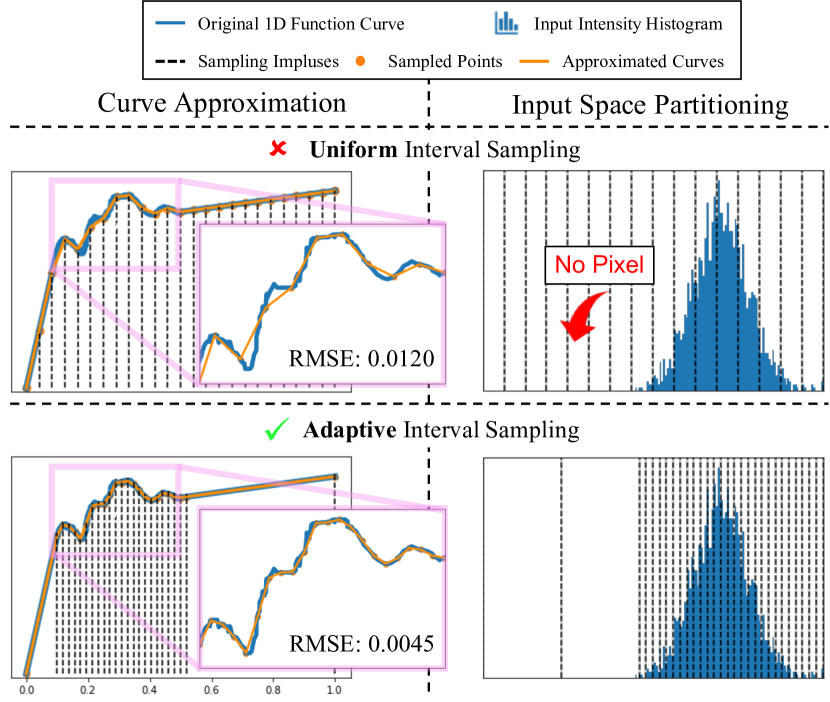
Figure 1: Comparison between uniform and non-uniform sampling on curve approximation and space partitioning. The illustration is given in 1D but can be easily extended to 3D.

Recent advances in machine learning techniques remarkably boosted the performance of automatic photo enhancement methods [48, 21, 19, 6, 9, 5], aiming to replace a sequence of meticulously-designed operations [43, 50, 25, 2, 33, 24] in the camera imaging pipeline [20] for enhanced visual quality. However, these methods suffer from heavy computational burdens due to complicated optimization processes [13, 49, 10, 21, 19] or neural architecture designs [6, 9, 47, 5]. In fact, most of the commonly-used enhancement operations are pixel-independent, as revisited in [17]. Their total effect is approximately equivalent to a 3D color transform function ($\mathbb{R}^{3}\rightarrow\mathbb{R}^{3}$) that maps an input color point to another one in or across the color spaces. One can adopt a multi-layer perceptron (MLP) to design such a transform [17] but requires a cascade of several linear and nonlinear sub-operations to increase the model capability. To overcome the computational complexity of a series of sub-operations in the transform, the 3D lookup table (LUT) is a promising data structure to conduct efficient mapping by sparsely sampling a range of input values and storing the corresponding output values in a 3D lattice. The non-linearities in the transform are typically approximated by a set of (tri-)linear interpolation functions distributed in the lattice cells. Since a LUT can transform images using only memory access and interpolation operations, it shows an advantage of high efficiency and practicality.

Previous works [51, 45] have made efforts to learn an image-adaptive LUT, mimicking the underlying optimal color transform with adaption to extensively varied image content. These methods embody the image-adaptiveness of the 3D LUTs only in the output color values, which are automatically learned by neural networks [51, 45]. However, they conduct sampling with equal intervals, not considering the adaption of sampling point density to image contents. It results in a sub-optimal sampling point allocation, limiting the expressiveness of the LUTs to model local non-linearities. Specifically, input pixels with similar color values but requiring highly non-linear contrast stretching (e.g., enhancement on low-light texture regions) are possibly compressed into the same lattice cell, which ends up producing linear-scaling results. The reasons lie in limited sampling points and (tri-)linear interpolation in the LUT transform. As depicted in the left part of Figure 1, for example, a uniform spacing undersamples a color range where the transform exhibits high curvature, resulting in distortion of the non-linearities in the transform. Ideally, increasing the number of sampling points might mitigate the issues but will significantly increase the overhead of the 3D LUT. Besides, it would also aggravate the oversampling in color space where few pixels fall into, causing waste in the LUT capacity, as shown in the right part of Figure 1.

To achieve a better tradeoff between effectiveness and efficiency when given limited sampling points, we develop a novel deep learning-based approach to adjust the layout of the 3D lattice by dynamically learning the non-uniform sampling intervals. This idea is encapsulated into a compact network module called AdaInt, that can adaptively allocate more sampling points to color ranges requiring highly non-linear transforms and reduce redundant sampling point quota for strongly linear ranges. As illustrated in Figure 2, with the incorporation of AdaInt, a lightweight convolutional neural network (CNN) takes a down-sampled image as input to simultaneously predict two components of a dedicated 3D LUT – the non-uniform sampling coordinates and the corresponding output color values. These two components are combined to compose an image-adaptive 3D LUT that transforms the original image via a novel differentiable operator called AiLUT-Transform, which can provide gradients to AdaInt for end-to-end learning. This operator is essential for locating input colors in a non-uniform 3D lattice by introducing a low-complexity binary search into the lookup procedure of a LUT transform. Therefore, our method could be a plug-and-play module for 3D LUTs and still presents high efficiency.

The main contributions of this paper are three-fold: (1) We view the learning of 3D LUTs from the viewpoint of sampling and point out the importance of the sampling strategy for modeling color transforms with higher non-linear capability. (2) We present a novel AdaInt module and the corresponding AiLUT-Transform operator to enable the adaptive learning of a 3D LUT with a non-uniform layout. (3) We demonstrate the effectiveness and efficiency of our method on two large-scale publicly available datasets.

2 Related Works

Figure 2: Framework of the proposed method. Our method employs a CNN model on the down-sampled version of the input image to simultaneously predict two fundamental components of an image-adaptive 3D LUT – the sampling coordinates and output values. These two components construct a dedicated 3D LUT in a non-uniform layout via the lattice creation and rendering processes. The input image of the original resolution can be afterward transformed by the predicted 3D LUT efficiently via a designed novel AiLUT-Transform. The overall framework can be trained under the supervision of the groundtruth images in an end-to-end manner. Best viewed in color.

2.1 Photo Enhancement Methods

Recent advances in learning-based image enhancement methods can be roughly divided into two categories. The first paradigm [6, 37, 9, 52, 47, 5] directly learns the dense end-to-end mapping via fully convolutional networks [32]. While this line of works can achieve promising results, they usually suffer from heavy computational and memory burdens, limiting their practicalities. The second paradigm simultaneously leverages the strong fitting abilities of deep learning and the high efficiency of traditional physical models. This line of studies commonly transfers the heavy CNN dense inference into light physical model parameter prediction. The physical models are then used to enhance original images efficiently. The frequently used physical models include affine color transforms [14, 44, 3, 31], mapping curves (which can be viewed as 1D LUTs) [38, 42, 22, 23, 28, 16, 39], multi-layer perceptrons (MLPs) [17] and 3D color LUTs [51, 45]. Among them, 3D LUT is the most promising one due to its faster speed than MLPs, along with the stronger capability than affine transforms and mapping curves. The works most related to ours are [51, 45], which also learn image-adaptive 3D LUTs for enhancing images in real-time. However, they learn 3D LUTs in a uniform layout without considering the image-adaptiveness of the sampling strategy, which restricts their ability to model non-linear color transform.

2.2 Non-uniform Sampling

Non-uniform sampling strategies have been extensively investigated in 3D shape recognition such as meshes [15], point clouds [41], and implicit function fields [35] due to their higher efficiency and expressiveness compared to regular grids. For 2D image analysis, while the dominant paradigm is computation on regular 2D grids, recent works have made attempts to the non-uniform sampling of the input images [34], output images [27], feature maps [7], and convolution filters [11]. These works showed that an adaptive sampling strategy enables a high-quality representation using fewer sampling points. Non-uniform layouts have also emerged in traditional LUT implementation [30, 4, 36]. However, these works focus on another task, lattice regression [12], aiming to fit a known color transform into a static 3D LUT and repeat the transform during inference. The non-uniform layouts are introduced as an alternative way to reduce estimation errors. However, these methods are not flexible and intelligent as the estimated LUT is fixed and cannot adapt to new samples. Instead, our work learns the non-uniform 3D LUTs based on the content of every single image for more intelligent enhancement.

3 Method

3.1 Preliminary: 3D Lookup Tables

In this paper, we view a 3D LUT as a discrete sampling of a complete 3D color transform function. The sampled results are stored in a 3D lattice of output color values $T=\{(T_{r,(i,j,k)},T_{g,(i,j,k)},T_{b,(i,j,k)})\}_{i,j,k\in\mathbb{I}_{0}^{N_{s}-1}}$ that can be queried by sets of input color coordinates $P=\{(P_{r,(i,j,k)},P_{g,(i,j,k)},P_{b,(i,j,k)}\}_{i,j,k\in\mathbb{I}_{0}^{N_{s}-1}}$, where $N_{s}$ is the number of sampling coordinates along each of three dimensions and $\mathbb{I}_{0}^{N_{s}-1}$ denotes the set of $\{0,1,\dots,N_{s}-1\}$. Such a lattice defines a total of $N_{s}^{3}$ sampling points on the complete 3D color transform function. Once a 3D lattice is sampled, an input pixel looks up its nearest sampling points according to its color and computes its transformed output via interpolation (typically trilinear interpolation).

Due to the high efficiency and stability of 3D LUTs, previous methods [51, 45] have tried creating automatic image enhancement tools by learning image-adaptive 3D LUTs. They predict image-adaptive output values $T\in[0,1]^{3\times N_{s}\times N_{s}\times N_{s}}$ by learning several basis 3D LUTs and fusing them using image-dependent weights. These weights are predicted by a CNN model from the down-sampled input image, which significantly saves the computational cost (see the left part of Figure 2). However, these methods uniformly discretize the 3D color space, not considering the image-adaptiveness of sampling coordinates $P\in[0,1]^{3\times N_{s}\times N_{s}\times N_{s}}$, making them suffer from sub-optimal sampling point allocation and limited LUT capability.

In this paper, we address the above issues by simultaneously learning the sampling coordinates and the corresponding output color values in an image-adaptive fashion. Figure 2 shows an overview of the proposed framework. We directly follow the practice in [51] to predict a set of candidate output color values $T$ due to its proven effectiveness. Suppose that $N_{s}$ sampling coordinates along each dimension and an input image $X\in[0,1]^{3\times H\times W}$ are given. The output color values of a LUT can be formulated as

$$T=h(f(X)),$$ (1)

where $f$ is a function mapping an input image into a compact vector representation $E\in\mathbb{R}^{F}$. The function $h$ takes $E$ as input and predicts all output color values in $T$. Note that we encapsulate the idea of learning $M$ image-independent basis 3D LUTs and $M$ image-adaptive weights [51] into a cascade of two mappings, denoted as $h:\mathbb{R}^{F}\xrightarrow[]{h_{0}}\mathbb{R}^{M}\xrightarrow[]{h_{1}}[0,1]^{3\times N_{s}\times N_{s}\times N_{s}}$, with the insight of using rank factorization to save parameters. The basis 3D LUTs are encoded as the parameters of $h_{1}$. Please refer to Section C.1 for more details. In the following section, we focus more on the learning of the sampling coordinates $P$.

3.2 Adaptive Intervals Learning (AdaInt)

Predicting the sampling color coordinates is equivalent to learning the placement of the sampling points in the 3D color space. Although the totally free sampling points placement provides high flexibility, it complicates the lookup procedure and increases the overhead significantly. To this end, we present a simple yet effective way to achieve the so-called constrained sampling point placement. First, we assume that the three lattice dimensions are independent of each other during the lookup procedure. In this way, we can predict the sampling coordinates along each lattice dimension separably. Second, we reparameterize the sampling coordinates by the intervals between each adjacent pair of them. Therefore, by converting the learning goal from sampling coordinates to sampling intervals, we propose a novel image-adaptive constrained sampling point placement method, termed AdaInt, which we illustrate in the following four steps.

Unnormalized Intervals Prediction

Our method first predicts different sets of $N_{s}-1$ unnormalized sampling intervals for three lattice dimensions, thus producing a total of $3\times(N_{s}-1)$ values of intervals:

$$\hat{Q}\in\mathbb{R}^{3\times(N_{s}-1)}=g(f(X)).$$ (2)

In this work, we share the mapping $f$ between sampling points prediction and output values prediction. $g$ denotes a mapping of $\mathbb{R}^{F}\rightarrow\mathbb{R}^{3\times(N_{s}-1)}$. Please refer to Section 4.2 for more implementation details.

Intervals Normalization

Since the input and output spaces are normalized, the intervals for a given dimension should also spread out in the range of $[0,1]$. In this work, we choose the softmax function to get the normalized intervals $Q\in[0,1]^{3\times(N_{s}-1)}=\text{softmax}(\hat{Q},\text{axis}=1)$ for convenience. The term ”$\text{axis}=1$” indicates the normalization is performed on each of three color dimensions separably.

Intervals to Coordinates Conversion

The sampling coordinates $\hat{P}\in[0,1]^{3\times N_{s}}$ are obtained by applying cumulative summation to $Q$ and prepending an origin to each lattice dimension, which can be formulated as: $\hat{P}=[0_{3}^{T};\text{cumsum}(Q,\text{axis}=1)]$, where $0_{3}$ is a 3-dimension zero vector, and the $[\cdot\ ;\ \cdot]$ symbol denotes the concatenation operation. The above operations guarantee the bounded ($0\leq\hat{P}_{c,i}\leq 1$, for $\forall c=r,g,b$ and $\forall i\in\mathbb{I}_{0}^{N_{s}-1}$) and the monotone increasing properties ($\hat{P}_{c,i}\leq\hat{P}_{c,j}$, for $\forall c=r,g,b$, and $\forall i,j\in\mathbb{I}_{0}^{N_{s}-1},i\leq j$) of the predicted sampling coordinates along each dimension, which significantly simplifies the lookup procedure to be presented in Section 3.3.

Non-uniform 3D Lattice Construction

The above $\hat{P}$ matrix indeed provides three $N_{s}$-dimension coordinate vectors for each lattice dimension, respectively. We can derive the 3D coordinates $P\in[0,1]^{3\times N_{s}\times N_{s}\times N_{s}}$ of the $N_{s}^{3}$ sampling points by calculating the n-ary Cartesian product ($\otimes$) over these $3$ coordinate vectors, i.e., $P=\hat{P}_{r}\otimes\hat{P}_{g}\otimes\hat{P}_{b}=\{(\hat{P}_{r,i},\hat{P}_{g,j},\hat{P}_{b,k})|i,j,k\in\mathbb{I}_{0}^{N_{s}-1}\}$. These coordinates determine the vertex locations of a non-uniform 3D lattice. The final 3D LUT is easily constructed by assigning each output color value in $T$ to the corresponding vertex defined in $P$. Such a procedure can be vividly analogized to a rendering process, as illustrated in Figure 2.

Figure 3: Procedure of the proposed AiLUT-Transform, which is achieved by two operations: lookup and interpolation. Best viewed in color.

3.3 Differentiable Adaptive Interval Lookup Table Transform (AiLUT-Transform)

With the involvement of AdaInt, the LUT transform should take both the output values $T$ and the sampling coordinates $P$ of the LUT, along with the input image $X$ to produce the transformed output image $\hat{Y}$. In the standard LUT transform, $P$ is usually omitted since the sampling coordinates are assumed uniform. Therefore, the gradient with respect to $P$ has not yet been explored, which hinders the end-to-end learning of AdaInt. To this end, we introduce a novel transform operation called AiLUT-Transform:

$$\hat{Y}=\text{AiLUT-Transform}(X,T,P).$$ (3)

The AiLUT-Transform is (sub-)differential with respect to not only $X$ and $T$, but also $P$. This enables the end-to-end learning of the AdaInt module. Given an input query pixel $x$ consisting of three color components $\{x_{r},x_{g},x_{b}\}$, AiLUT-Transform computes its transformed color via two basic steps: lookup and interpolation. Please also see Figure 3 for a graphic illustration.

The Lookup Step

Our AiLUT-Transform first performs a lookup operation to locate the query pixel in the 3D LUT. As shown in the top part of Figure 3, this operation aims to find both the left and right neighbors $x_{c}^{0},x_{c}^{1}\in P\ (c=r,g,b)$ along each dimension for the query pixel. It can be easily achieved by a binary search thanks to the bounded and the monotone increasing properties of our learned sampling coordinates (see Section 3.2). Accordingly, the $8$ adjacent points in the LUT can be queried using the indices of the located neighbors in $P$. For a sampling point corresponding to $x_{r}^{i},x_{g}^{j},x_{b}^{k}$, where $i,j,k\in\{0,1\}$, we abbreviate the output color values of these 8 neighbors as $\tilde{T}_{:,i,j,k}$.

The Interpolation Step

After querying 8 adjacent points, trilinear interpolation is conducted to compute the transformed output color of the query pixel. As shown in the bottom part of Figure 3, the transformed output $\hat{y}$ is the sum of the values at $8$ corners weighted by the normalized partial volume diagonally opposite the corners, which can be formulated as:

$$\begin{split}\hat{y}=\sum_{i,j,k\in\{0,1\}}V_{i,j,k}\cdot\tilde{T}_{:,i,j,k},\end{split}$$ (4)

where $V_{i,j,k}=(x_{r}^{d})^{i}(1-x_{r}^{d})^{1-i}(x_{g}^{d})^{j}(1-x_{g}^{d})^{1-j}(x_{b}^{d})^{k}(1-x_{b}^{d})^{1-k}$, and $x_{c}^{d}=(x_{c}-x_{c}^{0})/(x_{c}^{1}-x_{c}^{0})\ (c=r,g,b)$.

Backpropagation

To allow the learning of AdaInt via backpropagation, we derive the gradients with respect to $x_{c}^{0},x_{c}^{1}$, and therefore to $P$. The partial derivative of $x_{c}^{0}$ is:

$$\frac{\partial\hat{y}}{\partial x_{c}^{0}}=\sum_{i,j,k\in\{0,1\}}\tilde{T}_{:,i,j,k}\frac{\partial V_{i,j,k}}{\partial x_{c}^{d}}\frac{\partial x_{c}^{d}}{\partial x_{c}^{0}}$$ (5)

and similarly to Equation 5 for $x_{c}^{1}$. Please refer to Section B.2 for detailed derivation. Besides, the gradient with respect to $\tilde{T}_{:,i,j,k}$ is more concise: $\partial\hat{y}/\partial\tilde{T}_{:,i,j,k}=V_{i,j,k}$.

As the proposed AiLUT-Transform is applied to each pixel independently, it can be implemented efficiently via CUDA. We merge the lookup and interpolation operations into a single CUDA kernel to maximize parallelism. Since our lookup operation is achieved by the binary search algorithm of logarithmic time complexity ($\mathcal{O}(\log_{2}N_{s})$), its computational cost is negligible in our case, where $N_{s}$ has a relatively small value (typically, 33).

Figure 4: Ablation study on AdaInt under different numbers ($N_{s}$) of sampling coordinates. The results on the FiveK dataset (480p) [1] for tone mapping are plotted.

Sampling Strategy	PSNR$\uparrow$	SSIM$\uparrow$
Shared-AdaInt	25.13	0.921
AdaInt	25.28	0.925

Table 1: Ablation study on different sampling strategies in AdaInt. The results on the FiveK dataset (480p) [1] for tone mapping are listed. ”$\uparrow$” indicates the larger is better.

Method	#Parameters	480p				Full Resolution (4K)
		PSNR	SSIM	$\Delta E_{ab}$	Runtime	PSNR	SSIM	$\Delta E_{ab}$	Runtime
UPE [44]	927.1K	21.88	0.853	10.80	4.27	21.65	0.859	11.09	56.88
DPE [6]	3.4M	23.75	0.908	9.34	7.21	-	-	-	-
HDRNet [14]	483.1K	24.66	0.915	8.06	3.49	24.52	0.921	8.20	56.07
DeepLPF [37]	1.7M	24.73	0.916	7.99	32.12	-	-	-	-
CSRNet [17]	36.4K	25.17	0.924	7.75	3.09	24.82	0.926	7.94	77.10
SA-3DLUT [45]*	4.5M	25.50	/	/	2.27	/	/	/	4.39
3D-LUT [51]	593.5K	25.29	0.923	7.55	1.17	25.25	0.932	7.59	1.49
3D-LUT + AdaInt	619.7K	25.49	0.926	7.47	1.29	25.48	0.934	7.45	1.59

Table 2: Quantitative comparisons on the FiveK dataset  [1] for photo retouching. Runtime is measured in milliseconds. ”-” means the result is not available due to insufficient GPU memory. The ”*” symbol indicates that the results are adopted from the original paper (some are absent (”/”)) due to the unavailable source code. The best and second results are highlighted in red and blue, respectively.

3.4 Loss Function

The overall framework can be trained in an end-to-end manner. Our loss function consists of the MSE loss as the reconstruction loss ($\mathcal{L}_{r}$) and some regularization terms adopted from  [51] to constrain the output values $T$ of the LUT, including smoothness term ($\mathcal{L}_{s}$) and monotonicity term ($\mathcal{L}_{m}$). We do not introduce any other constraint or loss function to the learning of AdaInt, willing that it can be image-adaptive for the network. Following [51], our final loss is written as:

$$\mathcal{L}=\mathcal{L}_{r}+0.0001\times\mathcal{L}_{s}+10\times\mathcal{L}_{m}.$$ (6)

4 Experiments

Method	480p
	PSNR	SSIM	$\Delta E_{ab}$
UPE [44]	21.56	0.837	12.29
DPE [6]	22.93	0.894	11.09
HDRNet [14]	24.52	0.915	8.14
CSRNet [17]	25.19	0.921	7.63
3D-LUT [51]	25.07	0.920	7.55
3D-LUT + AdaInt	25.28	0.925	7.48

Table 3: Quantitative comparisons on the FiveK dataset (480p) [1] for the tone mapping application. The best and second results are highlighted in red and blue, respectively.

4.1 Datasets and Application Settings

We evaluate our method on two publicly available datasets: MIT-Adobe FiveK [1] and PPR10K [29]. The MIT-Adobe FiveK is a commonly used photo retouching dataset with 5,000 RAW images. We follow the common practice in recent works [51, 17, 22] to adopt only the version retouched by expert C as the groundtruth and split the dataset into 4,500 image pairs for training and 500 image pairs for testing. To speed up the training stage, images are downsampled to 480p resolution (with the short side resized to 480 pixels), whereas images of both 480p and original 4K resolutions are used during testing. The PPR10K is a newly released portrait photo retouching dataset with a larger scale of 11,161 high-quality RAW portrait photos. All three retouched versions are used as the groundtruth in three separable experiments. Following the official split [29], we divide the dataset into 8,875 pairs for training and 2,286 pairs for testing. Experiments are conducted on the 360p version of the dataset due to insufficient disk space. Please refer to Appendix C for more details.

We follow  [51] to conduct our experiments on two typical applications: photo retouching and tone mapping. The target images in both applications share the same 8-bit sRGB format. The difference between the two tasks lies in the input formats. In the photo retouching task, the input images are also in sRGB format (8-bit on FiveK and 16-bit on PPR10K), while for the tone mapping task, the input images are in 16-bit CIE XYZ format. Therefore, the tone mapping task requires the ability of color space conversion. We conduct both tasks on the FiveK dataset, but only the retouching task on PPR10K as done in [29].

Method	E	PSNR	$\Delta E_{ab}$	$\text{PSNR}^{\text{HC}}$	$\Delta E_{ab}^{\text{HC}}$
HDRNet [14]	a	23.93	8.70	27.21	5.65
CSRNet [17]	a	22.72	9.75	25.90	6.33
3D-LUT [51]	a	25.64	6.97	28.89	4.53
3D-LUT + HRP [29]	a	25.99	6.76	28.29	4.38
3D-LUT + AdaInt	a	26.33	6.56	29.57	4.26
HDRNet [14]	b	23.96	8.84	27.21	5.74
CSRNet [17]	b	23.76	8.77	27.01	5.68
3D-LUT [51]	b	24.70	7.71	27.99	4.99
3D-LUT + HRP [29]	b	25.06	7.51	28.36	4.85
3D-LUT + AdaInt	b	25.40	7.33	28.65	4.75
HDRNet [14]	c	24.08	8.87	27.32	5.76
CSRNet [17]	c	23.17	9.45	26.47	6.12
3D-LUT [51]	c	25.18	7.58	28.49	4.92
3D-LUT + HRP [29]	c	25.46	7.43	28.80	4.82
3D-LUT + AdaInt	c	25.68	7.31	28.93	4.76

Table 4: Quantitative comparisons on the PPR10K dataset [29] for portrait photo retouching, where ”E” denotes ”Expert”, and a, b, c indicate the groundtruths retouched by three experts.

Figure 5: Illustration of the learned sampling coordinates and the corresponding 3D LUTs for photo retouching on the PPR10K dataset (360p) [29]. The bottom row visualizes the learned sampling coordinates on the so-called per-color-channel Accumulative Error Histogram (AEH) [30]. The regions in the AEH exhibiting high curvature indicate wherein more sampling points are needed. Best viewed on screen.

4.2 Implementation Details

Since the focus of our work is to present the idea of learning image-adaptive sampling intervals for a 3D LUT, we do not dive into complicated architectural engineering. Instead, to instantiate the mapping $f$ in our method, we directly follow Zeng’s [51, 29] practices to adopt the 5-layer backbone in  [51] on the FiveK dataset and the ResNet-18 [18] (initialized with ImageNet-pretrained [8] weights) on the PPR10K dataset. The mapping $h$ in Equation 1 is implemented with two cascade fully-connected layers, which in practice reformulates the implementation in [51]. For the instantiation of AdaInt (mapping $g$ in Equation 2), a single fully-connected layer is employed. The weights and bias of $g$ are initialized to 0s and 1s, which makes the predicted sampling intervals start from a uniform state. Please refer to Appendix C for more details.

We use the standard Adam optimizer [26] to minimize the loss function in Equation 6. The mini-batch size is set to 1 and 16 on FiveK and PPR10K, respectively. All our models are trained for 400 epochs with a fixed learning rate of $1\times 10^{-4}$. We decay the learning rate of $g$ by a factor of 0.1 and freeze its parameters in the first 5 training epochs to make the AdaInt learning more stable. Our method is implemented based on PyTorch [40]. All experiments are conducted on an NVIDIA Tesla V100 GPU. The settings of $N_{s}$ and $M$ are according to the datasets and the experimental purposes. We provide them in the following sections.

4.3 Ablation Studies

In this section, the tone mapping task with images from the FiveK dataset (480p) is chosen to conduct several ablation studies for verifying the proposed AdaInt. We expect the higher dynamic range (16-bit) of the input images in the tone mapping task can better examine the ability of our AdaInt to learn image-adaptive sampling points. In all ablation studies, the hyper-parameter $M$ is set to 3.

Number of Coordinates along Each Dimension

We assess the baseline 3D-LUT [51] and our method under different settings of $N_{s}$ (the number of sampling coordinates along each color dimension) to verify the efficacy of the proposed AdaInt. As shown in Figure 4, the performance of the baseline and our method decrease as a smaller $N_{s}$ is adopted. Our AdaInt consistently improves the baseline under all settings $N_{s}$. Further increasing $N_{s}$ (from 33 to 65) can only bring marginal improvement (0.05dB) on the baseline compared with that introduced by our AdaInt. It is worth noting that our method achieves comparable or even better performance with a relatively small LUT size ($N_{s}$) compared to the baseline. It is because AdaInt enables the ability of 3D LUTs to take full advantage of the limited sampling points for better modeling on the underlying optimal color transform.

Sampling Strategy

Our AdaInt generates an individual set of sampling intervals for each color dimension separably, making our method adopts different sampling strategies along different color dimensions. It divides the entire 3D color space into various cuboids. Here, we compare such a default setting with another one that adopts the same strategy over three color dimensions, which divides the 3D space into cubes. We achieve it by letting AdaInt generate only a set of sampling intervals and replicate it to three color dimensions, abbreviated as Shared-AdaInt. As shown in Table 1, the Shared-AdaInt strategy performs inferior to the default setting, which is in line with our expectation as the sharing mechanism limits the flexibility of AdaInt to allocate sampling points in the 3D space.

Figure 6: Qualitative comparisons with corresponding error maps on the FiveK dataset [1] for photo retouching. Best viewed on screen.

4.4 Property of the Adaptive Sampling Intervals

The top part of Figure 5 shows two different photos on the PPR10K dataset, their color histograms, and the corresponding learned 3D LUTs from our model. It can be observed that both the color and layout of the 3D lattices vary with the different image content, indicating the image-adaptive property of our learned 3D LUTs. To better analyze the behavior of our AdaInt, we introduce the per-color-channel Accumulative Error Histogram (AEH) [30] between the input and groundtruth images. The regions with high curvature in the AEH, to some extent, indicate the complexity/local-nonlinearity of the underlying 3D color transform and hence require more sampling points. As shown in the bottom part of Figure 5, the sampling coordinates predicted by our AdaInt non-uniformly and adaptively distribute to different regions according to the transform complexity on various images and color channels. A detailed description of AEH and more visualization of learned intervals can be found in Appendix D.

4.5 Comparison with State-of-the-Arts

We also compare state-of-the-art real-time photo enhancement methods. $N_{s}$ is set to 33 as done in other 3D LUT-based approaches [51, 45] for fair comparisons. $M$ is set to 3 and 5 for the FiveK and PPR10K datasets, respectively, as done in [29].

Quantitative Comparisons

We compare the selected methods on PSNR, SSIM [46], the $L_{2}$-distance in CIE LAB color space ($\Delta E_{ab}$), and the inference speed. On PPR10K, we also include the human-centered measures [29] (denoted by the ”HC” superscript). We obtain the results of existing methods using their published codes and default configurations. All approaches are executed on an NVIDIA Tesla V100 GPU. For speed comparison, we measure the GPU inference time on 100 images and report the average. Table 2 lists the comparison on the FiveK for photo retouching. Our method outperforms others with relatively fewer parameters on both resolutions. Similar conclusions apply to Tables 3 and 4 on the FiveK for tone mapping and the PPR10K for portrait photo retouching, respectively. Especially, our AdaInt brings consistent improvement over 3D-LUT [51] on all datasets with a negligible computational cost increase, demonstrating its efficiency and effectiveness. It is worth noting that the concurrent study SA-3DLUT [45] promotes 3D LUTs by constructing pixel-wise LUTs at the cost of a significant model size increase (about 7 times) and a speed decrease (about 3 times). We believe SA-3DLUT equipped with our AdaInt can be further improved, though the source code is not yet publicly available.

Qualitative Comparisons

Figure 6 shows that our method produces more visually pleasing results than other methods. For example, our method better handles the overexposure of the image in the first row. In the second row, other methods suffer from poor saturation in the blue sky, resulting in hazy photos. Our AdaInt instead successfully produces the correct blue color and thus provides a cleaner result. Besides, when enhancing the brightness in the third row, our method preserves more rock texture. Please refer to Figures 9 and 10 for more comparisons.

5 Limitation and Conclusion

While our AdaInt promotes the expressiveness of 3D LUTs by providing image-adaptive sampling strategies, it still lacks spatial modeling and noise robustness. The 3D LUTs assume that each pixel is transformed independently according to its color without considering the locality. Hence, it is more suited for global enhancement and may produce less satisfactory results in areas requiring local tone mapping.  [45] provided a possible solution by constructing pixel-wise LUTs. Our method is orthogonal to and may also bring improvement over it. Besides, as our approach is based on pixel-wise mapping, heavy noise may also influence our results. Please refer to Figure 7 for some visual examples.

In this paper, we present AdaInt, a novel learning mechanism to promote learnable 3D LUTs for real-time image enhancement. The central idea is to introduce image-adaptive sampling intervals for learning a non-uniform 3D LUT layout. We develop AdaInt as a plug-and-play neural network module and propose a differentiable AiLUT-Transform operator encapsulating binary search and trilinear interpolation. Experimental results on two datasets demonstrate the superiority of our method over other state-of-the-art methods in terms of both performance and efficiency. In addition, we believe the viewpoint of non-uniform sampling on a complicated underlying transform function or representation is not limited to 3D LUTs and can also facilitate other applications, which we leave as our future work.

Appendix A Motivation of Using 3D LUT

Inspired by the practice in the image signal processor (ISP) [20], we adopt the 3D LUT instead of a more general mapping function (e.g., a multi-layer perceptron (MLP)) to model the $\mathbb{R}^{3}\rightarrow\mathbb{R}^{3}$ color transform function due to the consideration of efficiency and expressiveness. Specifically, if a static MLP is used, it is easy to learn an over smooth transform since the network needs to adapt to all images in the dataset. Therefore, the model might suffer from its limited expressiveness and diversity among images. Adopting an additional network for predicting the parameters of an MLP to enable image-adaptiveness is another alternative and has been investigated in CSRNet [17]. However, since an MLP requires a cascade of several linear and nonlinear sub-operations to increase the model capability, it suffers from a higher computational burden, especially on high-resolution inputs, as shown in Table 2 (48 times over our AdaInt on 4K resolution). Instead, our 3D LUT with learned adaptive intervals is able to achieve enhanced expressiveness and image-adaptiveness while still presenting high efficiency by directly recording and retrieving a complex transform via simple lookup and interpolation operations.

Appendix B Details of AiLUT-Transform

B.1 Forward

Given an input image denoted as $X\in[0,1]^{3\times H\times W}$, suppose an image-adaptive 3D LUT is learned, its output values and sampling coordinates are abbreviated as $T\in[0,1]^{3\times N_{s}\times N_{s}\times N_{s}}$ and $\hat{P}\in[0,1]^{3\times N_{s}}$, respectively. $N_{s}$ is the number of sampling coordinates along each lattice dimension. The AiLUT-Transform takes all of $X$, $T$, and $\hat{P}$ as inputs, and produces the transformed output image $\hat{Y}$:

$$\hat{Y}=\text{AiLUT-Transform}(X,T,\hat{P}).$$ (7)

The transform consists of a lookup step and an interpolation step. The former locates each input pixel of $X$ in the LUT, whereas the latter computes the corresponding output using the values of eight nearest neighborhood sampling points in $T$. Suppose an input query pixel $x$ is given, which is composed of three color components $\{x_{r},x_{g},x_{b}\}$, the transform on $x$ is performed in the following steps.

The Lookup Step

The transform first locates the query pixel $x$ into a lattice cell closed by 8 nearest neighborhood sampling points. These 8 points (or called vertices) are determined by 6 coordinates obtained by finding both the left and right neighbors $x_{c}^{0},x_{c}^{1}\in\hat{P}\ (c=r,g,b)$ along each lattice dimension, and their corresponding indices in the LUT $e_{c}^{0},e_{c}^{1}\in\mathbb{I}_{0}^{N_{s}-1}$. In a standard LUT transform where the 3D lattice is constructed with equal intervals $\Delta=1/(N_{s}-1)$, this can be easily achieved:

$$e_{c}^{0}=\lfloor\frac{x_{c}}{\Delta}\rfloor,e_{c}^{1}=e_{c}^{0}+1,$$

$$x_{c}^{0}=e_{c}^{0}\Delta,x_{c}^{1}=e_{c}^{1}\Delta,$$

where $\lfloor\cdot\rfloor$ is the floor function. It is obvious that the $\hat{P}$ is not needed in the standard LUT transform, so it is always omitted in existing implementations. However, in AiLUT-Transform, since the intervals are no longer a constant value, a searching algorithm on $\hat{P}$ is required to find $x_{c}^{0},x_{c}^{1}$ and $e_{c}^{0},e_{c}^{1}$, which can be formulated as:

$$\begin{split}x_{c}^{0},e_{c}^{0}&=\max\{\hat{P}_{c,s},s|\hat{P}_{c,s}\leq x_{c},s\in\mathbb{I}_{0}^{N_{s}-1}\},\\ x_{c}^{1},e_{c}^{1}&=\min\{\hat{P}_{c,s},s|\hat{P}_{c,s}>x_{c},s\in\mathbb{I}_{0}^{N_{s}-1}\}.\end{split}$$ (8)

Thanks to the bounded and monotone increasing properties of the learned sampling coordinates stored in $\hat{P}$ (see Section 3.2), Equation 8 can be easily achieved by introducing a binary search.

Once the 6 indices ($e_{r}^{0},e_{r}^{1};e_{g}^{0},e_{g}^{1};e_{b}^{0},e_{b}^{1}$) for the nearest neighborhood vertices in the LUT are determined, the corresponding output color values of the 8 neighbors in $T$ can be defined as:

$$\tilde{T}_{:,i,j,k}=T[:,e_{r}^{i},e_{g}^{j},e_{b}^{k}],\ i,j,k\in\{0,1\}.$$ (9)

The Interpolation Step

After querying 8 adjacent vertices in the LUT for query pixel $x$, the transformed result can be obtained by applying trilinear interpolation, including the following steps:

• Compute the normalized offsets between the input color and the 8 neighbors:

  $$x_{r}^{d}=\frac{x_{r}-x_{r}^{0}}{x_{r}^{1}-x_{r}^{0}},x_{g}^{d}=\frac{x_{g}-x_{g}^{0}}{x_{g}^{1}-x_{g}^{0}},x_{b}^{d}=\frac{x_{b}-x_{b}^{0}}{x_{b}^{1}-x_{b}^{0}}.$$ (10)

• Compute the interpolation weights, which are defined as the partial volume diagonally opposite the vertices:

  $$\begin{split}V_{i,j,k}=&(x_{r}^{d})^{i}(1-x_{r}^{d})^{1-i}\\ &\cdot(x_{g}^{d})^{j}(1-x_{g}^{d})^{1-j}\\ &\cdot(x_{b}^{d})^{k}(1-x_{b}^{d})^{1-k}.\end{split}$$ (11)

• Compute the linear combination of $V_{i,j,k}$ and $\tilde{T}_{:,i,j,k}$:

  $$\hat{y}=\sum_{i,j,k\in\{0,1\}}V_{i,j,k}\cdot\tilde{T}_{:,i,j,k}.$$ (12)

B.2 Backpropagation

In our method, both $T$ and $\hat{P}$ are learned by neural networks to enable more flexible 3D LUT with adaption to different image content. The challenge exists in the absence of interpolation implementation in popular deep learning libraries (such as PyTorch [40]) that can provide gradients to $\hat{P}$. To this end, we provide a new implementation that can compute the gradients with respect to $\hat{P}$ during backpropagation to enable the end-to-end learning of AdaInt. The core is to define the partial derivatives of $x_{c}^{0},x_{c}^{1}$:

$$\begin{split}\frac{\partial\hat{y}}{\partial x_{c}^{0}}=\sum_{i,j,k\in\{0,1\}}\tilde{T}_{:,i,j,k}\frac{\partial V_{i,j,k}}{\partial x_{c}^{d}}\frac{\partial x_{c}^{d}}{\partial x_{c}^{0}},\\ \frac{\partial\hat{y}}{\partial x_{c}^{1}}=\sum_{i,j,k\in\{0,1\}}\tilde{T}_{:,i,j,k}\frac{\partial V_{i,j,k}}{\partial x_{c}^{d}}\frac{\partial x_{c}^{d}}{\partial x_{c}^{1}}.\end{split}$$ (13)

where,

$$\begin{split}\frac{\partial V_{i,j,k}}{\partial x_{r}^{d}}=(-1)^{1-i}\cdot(x_{g}^{d})^{j}(1-x_{g}^{d})^{1-j}\cdot(x_{b}^{d})^{k}(1-x_{b}^{d})^{1-k},\\ \frac{\partial V_{i,j,k}}{\partial x_{g}^{d}}=(x_{r}^{d})^{i}(1-x_{r}^{d})^{1-i}\cdot(-1)^{1-j}\cdot(x_{b}^{d})^{k}(1-x_{b}^{d})^{1-k},\\ \frac{\partial V_{i,j,k}}{\partial x_{b}^{d}}=(x_{r}^{d})^{i}(1-x_{r}^{d})^{1-i}\cdot(x_{g}^{d})^{j}(1-x_{g}^{d})^{1-j}\cdot(-1)^{1-k},\end{split}$$ (14)

and,

$$\begin{split}\frac{\partial x_{r}^{d}}{\partial x_{r}^{0}}=-\frac{1-x_{r}^{d}}{x_{r}^{1}-x_{r}^{0}},\ \frac{\partial x_{r}^{d}}{\partial x_{r}^{1}}=-\frac{x_{r}^{d}}{x_{r}^{1}-x_{r}^{0}},\\ \frac{\partial x_{g}^{d}}{\partial x_{g}^{0}}=-\frac{1-x_{g}^{d}}{x_{g}^{1}-x_{g}^{0}},\ \frac{\partial x_{g}^{d}}{\partial x_{g}^{1}}=-\frac{x_{g}^{d}}{x_{g}^{1}-x_{g}^{0}},\\ \frac{\partial x_{b}^{d}}{\partial x_{b}^{0}}=-\frac{1-x_{b}^{d}}{x_{b}^{1}-x_{b}^{0}},\ \frac{\partial x_{b}^{d}}{\partial x_{b}^{1}}=-\frac{x_{b}^{d}}{x_{b}^{1}-x_{b}^{0}}.\end{split}$$ (15)

Note that since $x_{c}^{0},x_{c}^{1}$ are elements in $\hat{P}$, Equations 13, 14 and 15 indeed define the partial derivatives with respect to $\hat{P}$, allowing the loss gradients to flow back to the sampling coordinates, and therefore back to the sampling intervals and any preceding neural network modules. The AiLUT-Transform works on each pixel independently, so it is highly parallelizable, especially on GPUs.

Appendix C Experimental Details

Both datasets used in our work, i.e., the MIT-Adobe FiveK [1] and PPR10K [29], are publicly released, free of charge for research use, and contain no personally identifiable information. We conducted our experiments based on PyTorch 1.8.1 [40] and the MMEditing toolbox (v0.11.0, under Apache 2.0 license) . The proposed AiLUT-Transform is complied as a PyTorch CUDA extension using CUDA 10.2. In the following section, we provide more experimental details about these two datasets.

C.1 FiveK

Datasets Preprocessing

Experiments on the FiveK dataset are conducted on two different resolutions (480p and 4K) and two different applications (retouching and tone mapping). For retouching and tone mapping on 480p, we directly download the dataset released by [51] for model training and testing. To obtain the original 4K images, we follow [51] to download the original dataset and use the Adobe Lightroom software to pre-process the RAW images. We use the same training/testing splits as [51] to divide the dataset into 4500 training pairs and 500 testing pairs. For the sake of research reproducibility, we provide the split files and the detailed instruction of data pre-processing at https://github.com/ImCharlesY/AdaInt.

We train all our models on the 480p resolution. During training, input images (8-bit sRGB for retouching and 16-bit CIE XYZ for tone mapping) are normalized to $[0,1]$ for unified processing and are randomly augmented to mitigate overfitting and facilitate performance. The augmentations include random ratio cropping, random horizontal flipping, and random color jittering. The trained models can be directly applied to the original 4K resolution without performance drop (see Table 2). This protocol significantly speeds up the training stage and also demonstrates the flexibility and scalability of our method.

Id	Layer	Output Feature Shape
0	Bilinear Resize	$3\times 256\times 256$
1	Conv3x3, LeakyReLU	$16\times 128\times 128$
2	InstanceNorm	$16\times 128\times 128$
3	Conv3x3, LeakyReLU	$32\times 64\times 64$
4	InstanceNorm	$32\times 64\times 64$
5	Conv3x3, LeakyReLU	$64\times 32\times 32$
6	InstanceNorm	$64\times 32\times 32$
7	Conv3x3, LeakyReLU	$128\times 16\times 16$
8	InstanceNorm	$128\times 16\times 16$
9	Conv3x3, LeakyReLU	$128\times 8\times 8$
10	Dropout (0.5)	$128\times 8\times 8$
11	AveragePooling	$128\times 2\times 2$
12	Reshape	$512$

Table 5: Network architecture of the backbone module (the mapping $f$ in the paper) on the FiveK [1] dataset.

Model Architectures

The model architectures employed on the FiveK experiments are listed in Tables 5, 6 and 7. For the backbone network (mapping $f$), we directly adopt the 5-layer backbone in [51]. The mapping $h$ uses a cascade of two fully-connected (FC) layers, which reformulates the implementation in [51], i.e., the first FC layer (mapping $h_{0}$) is responsible for predicting $M$ input-dependent fusing weights, whereas the second FC layer (mapping $h_{1}$) encodes the parameters of $M$ basis 3D LUT. For the instantiation of mapping $g$, a single FC layer is adopted. We follow [51] to initialize the parameters of $f$ and $h$. As for the proposed AdaInt module (mapping $g$), we initialize its weights and bias to all 0s and 1s, which makes the predicted sampling intervals start from a uniform state, hence stabilizing the training of AdaInt.

Training Details

We train our models for 400 epochs with a fixed learning rate of $1\times 10^{-4}$ using the standard Adam optimizer [26]. The mini-batch size is set to 1. To further stabilize the AdaInt learning and facilitate the learning of more output color values in the 3D lattice, we decay the learning rate of $g$ by a factor of 0.1 and freeze its parameters in the first 5 training epochs.

Id	Layer	Output Feature Shape
0	FC	$M$
1	FC	$3N_{s}^{3}$
2	Reshape	$3\times N_{s}\times N_{s}\times N_{s}$

Table 6: Network architecture of the mapping $h$ in the paper. ”FC” denotes the fully-connected layer.

Id	Layer	Output Feature Shape
0	FC	$3(N_{s}-1)$
1	Reshape	$3\times(N_{s}-1)$
2	Softmax	$3\times(N_{s}-1)$
3	Cumsum	$3\times(N_{s}-1)$
4	ZeroPad	$3\times N_{s}$

Table 7: Network architecture of the mapping $g$ in the paper. ”FC” denotes the fully-connected layer, and ”Cumsum” is the operation to conduct cumulative summation.

C.2 PPR10K

Datasets Preprocessing

Experiments on the PPR10K dataset are conducted on the 360p resolution for the photo retouching application. The official training/testing ($8,875:2,286$) splits are adopted. During training, images augmented by the dataset creator are used as our inputs. Please refer to [29] for more details. Besides the pre-augmentations, we further apply some commonly-used data augmentation methods such as random ratio cropping and random horizontal flipping. Since the dataset is relatively larger-scale than the FiveK dataset, images are also resized into a unified $448\times 448$ resolution to enable mini-batch processing for speeding up the training stage.

Model Architectures

For experiments on the PPR10K dataset, the mapping $g$ and $h$ share identical architectures (Tables 7 and 6) with those on the FiveK dataset. For the backbone network (the mapping $f$), we follow [29] to adopt the ResNet-18 [18] (with a preceding bilinear layer resizing images into $224\times 224$ resolution) for a fair comparison. The initializations of $g$ and $h$ are the same as those in the FiveK experiments, whereas the ResNet-18 backbone is initialized using ImageNet [8] pretrained weights.

Training Details

We train our models for 200 epochs with a mini-batch size of 16 to speed up the training stage on such a large-scale dataset. For other settings, they are kept consistent with those in the FiveK experiments.

Figure 7: Qualitative results on noisy images for photo retouching on the FiveK dataset (480p) [51]. Best viewed on screen.

Appendix D More Visualization of AdaInt

To better investigate the behavior of AdaInt, inspired by [30], we introduce the per-color-channel Accumulative Error Histogram (AEH), which, to some extent, can indicate locations in the color ranges where more dense sampling points are required.

The AEH bins the intensity changes between input and target images according to the values of the input pixels. Therefore, it indicates the intensity change required for each input pixel value to transform the image. Given an input image $X\in[0,1]^{3\times H\times W}$ and the corresponding groundtruth image $Y\in[0,1]^{3\times H\times W}$, the AEH is constructed by first calculating the error map $D$ between $X$ and $Y$:

$$D_{c,h,w}=(X_{c,h,w}-Y_{c,h,w})^{2},$$ (16)

where $c=\{r,g,b\}$, $h\in\mathbb{I}_{0}^{H-1}$, and $w\in\mathbb{I}_{0}^{W-1}$. Before computing the histogram, we divide the input color range $[0,1]$ for a single channel uniformly into $N_{\text{bin}}$ bins and assign each input pixel into one of them according to its value at the corresponding color channel:

$$\Omega_{c}^{k}=\{X_{c,h,w}|k\Delta\leq X_{c,h,w}<(k+1)\Delta\},$$ (17)

where $\Delta=1/N_{\text{bin}}$ and $\Omega_{c}^{k}$ is the $k$-th bin ($k\in\mathbb{I}_{0}^{N_{\text{bin}}-1}$) for channel $c$. The normalized error histogram $H_{c}$ for channel $c$ is then computed as:

$$H_{c}[k]=\frac{1}{\Theta_{c}}\sum_{X_{c,h,w}\in\Omega_{c}^{k}}D_{c,h,w},$$ (18)

where $\Theta_{c}$ is a normalization term such that $\sum_{k}H_{c}[k]=1$. The final per-color-channel AEH can be easily derived by applying accumulative summation on $H_{c}$. In this work, we set $N_{\text{bin}}=1000$. The AEH can be visualized as a 1D curve as shown in Figure 8. The partial curve exhibiting higher curvature shows the color range requires a more substantial intensity change. Though not precise, the AEH indicates regions in the color range where the non-linearity is most prominent, and hence more sampling points are required.

We provide more visualization in Figure 8 of the learned sampling coordinates and the corresponding 3D LUTs for different images from the PPR10K dataset. It is clearly shown that the learned sampling coordinates are inclined to locate densely in the color range where the AEH exhibits high curvature, which suggests that our AdaInt is able to capture the complexity of the underlying optimal color transform with the adaption to the image content and achieve a more optimal sampling point allocation.

Appendix E Additional Qualitative Comparisons

In this section, we provide additional visual comparisons on the FiveK (4K) dataset in Figure 9 and on the PPR10K (360p) dataset in Figure 10.

Appendix F Real-time Performance on 8K Images

We also follow the protocol in [51] to resize the images into 8K (7680$\times$4320) resolution and measure the GPU inference time of both the baseline [51] and our method on a V100 GPU. The baseline can execute at a speed of 2.36 ms per 8K image, while AdaInt only increases the runtime to 2.54 ms, which still exceeds the requirement of real-time processing by a large margin. Note that the high efficiency of our method mainly owns to the characteristic that the computational cost of the CNN network is fixed as it operates on a downsampled, fixed-resolution version of the input, and the proposed AiLUT-Transform can be highly parallelized via customized CUDA code.

Appendix G Limitation

As discussed in Section 5, the proposed method is based on pixel-wise mapping and thus may fail to tackle heavy noise existing in the input. For verification, we randomly select three images from the FiveK dataset [1] and add Gaussian noise (with a standard deviation of $\sigma=0.02$) to them. As shown in Figure 7, both the baseline [51] and our method could not eliminate the added noise due to the lack of filtering capability. Constructing pixel-wise LUTs [45] might be a possible solution but still requires careful investigation to prevent substantial increases in memory and computational costs.

Appendix H Broader Impacts

The proposed method mimics the retouching style of human annotators based on learned statistics of the training dataset and as such will reflect biases in those data, including ones with negative societal impacts. Besides, there is no guarantee that the transformed colors by the method will please everybody due to the subjectiveness of the image/photo enhancement task. A possible mitigation strategy is to concern the preference of specific downstream users and retrains the method accordingly.

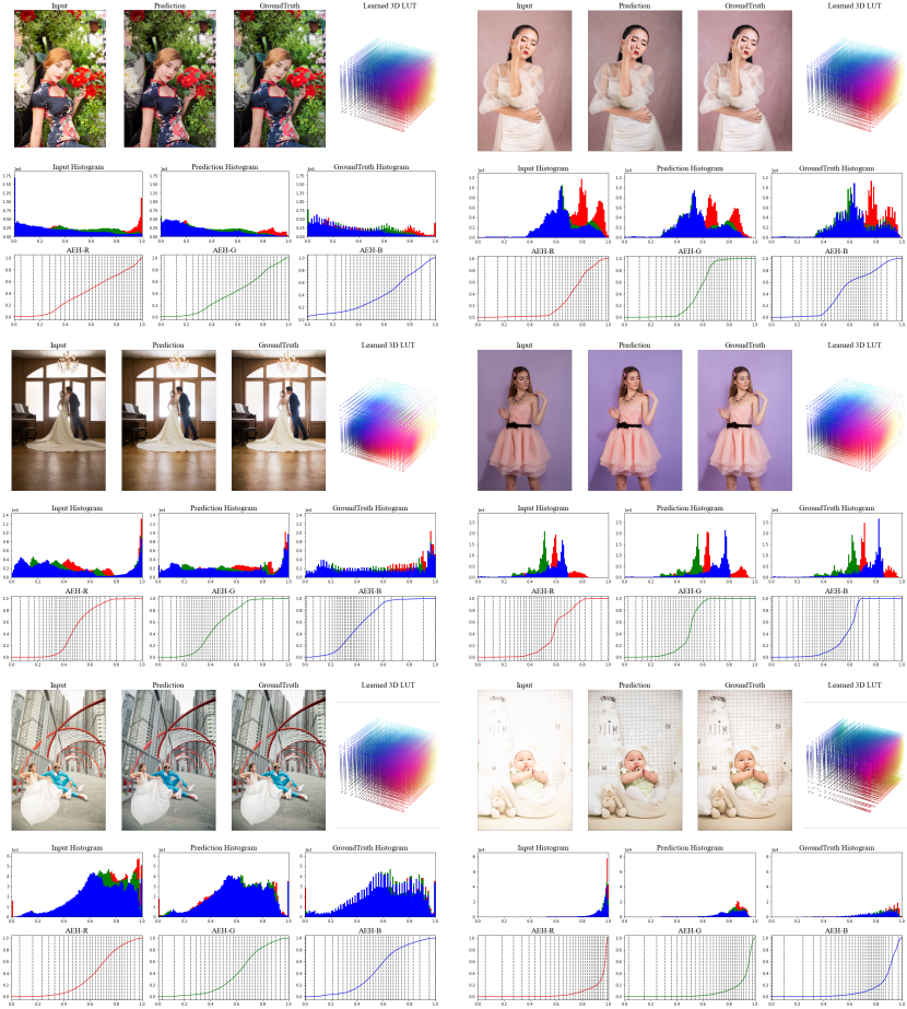
Figure 8: Illustration of the learned sampling coordinates and the corresponding 3D LUTs for photo retouching on the PPR10K dataset (360p) [29]. The bottom row visualizes the learned sampling coordinates on the so-called per-color-channel Accumulative Error Histogram (AEH) [30]. The regions in the AEH exhibiting high curvature indicate wherein more sampling points are needed. Best viewed on screen.

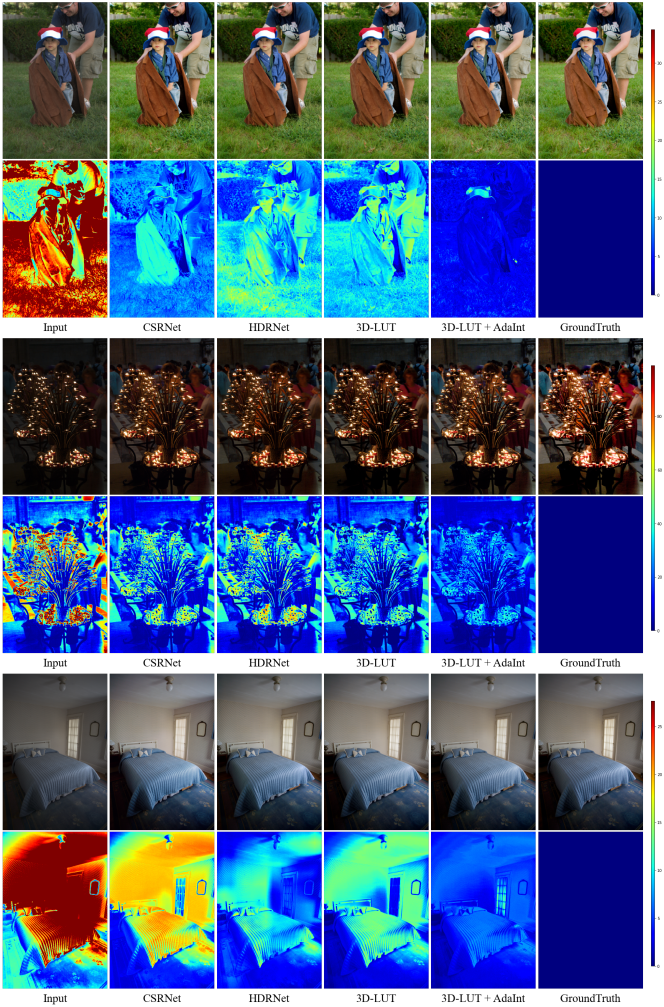
Figure 9: Additional qualitative comparisons of different methods for photo retouching on the FiveK dataset (4K) [1], and the corresponding error maps. Best viewed in zoom in.

Figure 10: Additional qualitative comparisons of different methods for photo retouching on the PPR10K dataset (360p) [1], and the corresponding error maps. Best viewed in zoom in.

References

- [1] Vladimir Bychkovsky, Sylvain Paris, Eric Chan, and Frédo Durand. Learning photographic global tonal adjustment with a database of input / output image pairs. In The Twenty-Fourth IEEE Conference on Computer Vision and Pattern Recognition, 2011.
- [2] Jianrui Cai, Shuhang Gu, and Lei Zhang. Learning a deep single image contrast enhancer from multi-exposure images. IEEE Transactions on Image Processing, 27(4):2049–2062, 2018.
- [3] Yoav Chai, Raja Giryes, and Lior Wolf. Supervised and unsupervised learning of parameterized color enhancement. In Proceedings of the IEEE/CVF Winter Conference on Applications of Computer Vision, pages 992–1000, 2020.
- [4] JZ Chan, Jan P Allebach, and Charles A Bouman. Sequential linear interpolation of multidimensional functions. IEEE Transactions on Image Processing, 6(9):1231–1245, 1997.
- [5] Chen Chen, Qifeng Chen, Jia Xu, and Vladlen Koltun. Learning to see in the dark. In Proceedings of the IEEE Conference on Computer Vision and Pattern Recognition, pages 3291–3300, 2018.
- [6] Yu-Sheng Chen, Yu-Ching Wang, Man-Hsin Kao, and Yung-Yu Chuang. Deep photo enhancer: Unpaired learning for image enhancement from photographs with gans. In Proceedings of the IEEE Conference on Computer Vision and Pattern Recognition, pages 6306–6314, 2018.
- [7] Jifeng Dai, Haozhi Qi, Yuwen Xiong, Yi Li, Guodong Zhang, Han Hu, and Yichen Wei. Deformable convolutional networks. In Proceedings of the IEEE international conference on computer vision, pages 764–773, 2017.
- [8] Jia Deng, Wei Dong, Richard Socher, Li-Jia Li, Kai Li, and Li Fei-Fei. Imagenet: A large-scale hierarchical image database. In 2009 IEEE conference on computer vision and pattern recognition, pages 248–255. Ieee, 2009.
- [9] Yubin Deng, Chen Change Loy, and Xiaoou Tang. Aesthetic-driven image enhancement by adversarial learning. In Proceedings of the 26th ACM international conference on Multimedia, pages 870–878, 2018.
- [10] Xueyang Fu, Delu Zeng, Yue Huang, Xiao-Ping Zhang, and Xinghao Ding. A weighted variational model for simultaneous reflectance and illumination estimation. In Proceedings of the IEEE conference on computer vision and pattern recognition, pages 2782–2790, 2016.
- [11] Hang Gao, Xizhou Zhu, Stephen Lin, and Jifeng Dai. Deformable kernels: Adapting effective receptive fields for object deformation. In 8th International Conference on Learning Representations, ICLR 2020, Addis Ababa, Ethiopia, April 26-30, 2020. OpenReview.net, 2020.
- [12] Eric Garcia and Maya Gupta. Lattice regression. Advances in Neural Information Processing Systems, 22:594–602, 2009.
- [13] Peter Vincent Gehler, Carsten Rother, Andrew Blake, Tom Minka, and Toby Sharp. Bayesian color constancy revisited. In 2008 IEEE Conference on Computer Vision and Pattern Recognition, pages 1–8. IEEE, 2008.
- [14] Michaël Gharbi, Jiawen Chen, Jonathan T Barron, Samuel W Hasinoff, and Frédo Durand. Deep bilateral learning for real-time image enhancement. ACM Transactions on Graphics (TOG), 36(4):1–12, 2017.
- [15] Georgia Gkioxari, Jitendra Malik, and Justin Johnson. Mesh r-cnn. In Proceedings of the IEEE/CVF International Conference on Computer Vision, pages 9785–9795, 2019.
- [16] Chunle Guo, Chongyi Li, Jichang Guo, Chen Change Loy, Junhui Hou, Sam Kwong, and Runmin Cong. Zero-reference deep curve estimation for low-light image enhancement. In Proceedings of the IEEE/CVF Conference on Computer Vision and Pattern Recognition, pages 1780–1789, 2020.
- [17] Jingwen He, Yihao Liu, Yu Qiao, and Chao Dong. Conditional sequential modulation for efficient global image retouching. arXiv preprint arXiv:2009.10390, 2020.
- [18] Kaiming He, Xiangyu Zhang, Shaoqing Ren, and Jian Sun. Deep residual learning for image recognition. In Proceedings of the IEEE conference on computer vision and pattern recognition, pages 770–778, 2016.
- [19] Sung Ju Hwang, Ashish Kapoor, and Sing Bing Kang. Context-based automatic local image enhancement. In European conference on computer vision, pages 569–582. Springer, 2012.
- [20] Hakki Can Karaimer and Michael S Brown. A software platform for manipulating the camera imaging pipeline. In European Conference on Computer Vision, pages 429–444. Springer, 2016.
- [21] Liad Kaufman, Dani Lischinski, and Michael Werman. Content-aware automatic photo enhancement. In Computer Graphics Forum, volume 31, pages 2528–2540. Wiley Online Library, 2012.
- [22] Hanul Kim, Su-Min Choi, Chang-Su Kim, and Yeong Jun Koh. Representative color transform for image enhancement. In Proceedings of the IEEE/CVF International Conference on Computer Vision, pages 4459–4468, 2021.
- [23] Han-Ul Kim, Young Jun Koh, and Chang-Su Kim. Global and local enhancement networks for paired and unpaired image enhancement. In European Conference on Computer Vision, pages 339–354. Springer, 2020.
- [24] Seon Joo Kim, Hai Ting Lin, Zheng Lu, Sabine Süsstrunk, Stephen Lin, and Michael S Brown. A new in-camera imaging model for color computer vision and its application. IEEE Transactions on Pattern Analysis and Machine Intelligence, 34(12):2289–2302, 2012.
- [25] Yeong-Taeg Kim. Contrast enhancement using brightness preserving bi-histogram equalization. IEEE transactions on Consumer Electronics, 43(1):1–8, 1997.
- [26] Diederik P. Kingma and Jimmy Ba. Adam: A method for stochastic optimization. In Yoshua Bengio and Yann LeCun, editors, 3rd International Conference on Learning Representations, ICLR 2015, San Diego, CA, USA, May 7-9, 2015, Conference Track Proceedings, 2015.
- [27] Alexander Kirillov, Yuxin Wu, Kaiming He, and Ross Girshick. Pointrend: Image segmentation as rendering. In Proceedings of the IEEE/CVF conference on computer vision and pattern recognition, pages 9799–9808, 2020.
- [28] Chongyi Li, Chunle Guo, Qiming Ai, Shangchen Zhou, and Chen Change Loy. Flexible piecewise curves estimation for photo enhancement. arXiv preprint arXiv:2010.13412, 2020.
- [29] Jie Liang, Hui Zeng, Miaomiao Cui, Xuansong Xie, and Lei Zhang. Ppr10k: A large-scale portrait photo retouching dataset with human-region mask and group-level consistency. In Proceedings of the IEEE Conference on Computer Vision and Pattern Recognition, 2021.
- [30] Hai Ting Lin, Zheng Lu, Seon Joo Kim, and Michael S Brown. Nonuniform lattice regression for modeling the camera imaging pipeline. In European Conference on Computer Vision, pages 556–568. Springer, 2012.
- [31] Enyu Liu, Songnan Li, and Shan Liu. Color enhancement using global parameters and local features learning. In Proceedings of the Asian Conference on Computer Vision, 2020.
- [32] Jonathan Long, Evan Shelhamer, and Trevor Darrell. Fully convolutional networks for semantic segmentation. In Proceedings of the IEEE conference on computer vision and pattern recognition, pages 3431–3440, 2015.
- [33] Rafał Mantiuk, Scott Daly, and Louis Kerofsky. Display adaptive tone mapping. ACM Trans. Graph., 27(3):1–10, Aug. 2008.
- [34] Dmitrii Marin, Zijian He, Peter Vajda, Priyam Chatterjee, Sam Tsai, Fei Yang, and Yuri Boykov. Efficient segmentation: Learning downsampling near semantic boundaries. In Proceedings of the IEEE/CVF International Conference on Computer Vision, pages 2131–2141, 2019.
- [35] Lars Mescheder, Michael Oechsle, Michael Niemeyer, Sebastian Nowozin, and Andreas Geiger. Occupancy networks: Learning 3d reconstruction in function space. In Proceedings of the IEEE/CVF Conference on Computer Vision and Pattern Recognition, pages 4460–4470, 2019.
- [36] Vishal Monga and Raja Bala. Sort-select-damp: An efficient strategy for color look-up table lattice design. In Color and Imaging Conference, volume 2008, pages 247–253. Society for Imaging Science and Technology, 2008.
- [37] Sean Moran, Pierre Marza, Steven McDonagh, Sarah Parisot, and Gregory Slabaugh. Deeplpf: Deep local parametric filters for image enhancement. In Proceedings of the IEEE/CVF Conference on Computer Vision and Pattern Recognition (CVPR), June 2020.
- [38] Sean Moran, Steven McDonagh, and Gregory Slabaugh. Curl: Neural curve layers for global image enhancement. In 2020 25th International Conference on Pattern Recognition (ICPR), pages 9796–9803. IEEE, 2021.
- [39] Jongchan Park, Joon-Young Lee, Donggeun Yoo, and In So Kweon. Distort-and-recover: Color enhancement using deep reinforcement learning. In Proceedings of the IEEE Conference on computer vision and pattern recognition, pages 5928–5936, 2018.
- [40] Adam Paszke, Sam Gross, Francisco Massa, Adam Lerer, James Bradbury, Gregory Chanan, Trevor Killeen, Zeming Lin, Natalia Gimelshein, Luca Antiga, Alban Desmaison, Andreas Kopf, Edward Yang, Zachary DeVito, Martin Raison, Alykhan Tejani, Sasank Chilamkurthy, Benoit Steiner, Lu Fang, Junjie Bai, and Soumith Chintala. Pytorch: An imperative style, high-performance deep learning library. In H. Wallach, H. Larochelle, A. Beygelzimer, F. d'Alché-Buc, E. Fox, and R. Garnett, editors, Advances in Neural Information Processing Systems 32, pages 8024–8035. Curran Associates, Inc., 2019.
- [41] Charles R Qi, Hao Su, Kaichun Mo, and Leonidas J Guibas. Pointnet: Deep learning on point sets for 3d classification and segmentation. In Proceedings of the IEEE conference on computer vision and pattern recognition, pages 652–660, 2017.
- [42] Yuda Song, Hui Qian, and Xin Du. Starenhancer: Learning real-time and style-aware image enhancement. In Proceedings of the IEEE/CVF International Conference on Computer Vision, pages 4126–4135, 2021.
- [43] Yoshiharu Takahashi, Yasutoshi Fujii, Keiichi Kawazu, Seiichi Isoguchi, Kohichi Yamaguchi, and Katsuya Nagaishi. Photographic film reproducing apparatus using object brightness and exposure correction amount to develop photographed images, May 5 1998. US Patent 5,748,287.
- [44] Ruixing Wang, Qing Zhang, Chi-Wing Fu, Xiaoyong Shen, Wei-Shi Zheng, and Jiaya Jia. Underexposed photo enhancement using deep illumination estimation. In Proceedings of the IEEE/CVF Conference on Computer Vision and Pattern Recognition, pages 6849–6857, 2019.
- [45] Tao Wang, Yong Li, Jingyang Peng, Yipeng Ma, Xian Wang, Fenglong Song, and Youliang Yan. Real-time image enhancer via learnable spatial-aware 3d lookup tables. In Proceedings of the IEEE/CVF International Conference on Computer Vision, pages 2471–2480, 2021.
- [46] Zhou Wang, Alan C Bovik, Hamid R Sheikh, and Eero P Simoncelli. Image quality assessment: from error visibility to structural similarity. IEEE transactions on image processing, 13(4):600–612, 2004.
- [47] Chen Wei, Wenjing Wang, Wenhan Yang, and Jiaying Liu. Deep retinex decomposition for low-light enhancement. In British Machine Vision Conference 2018, BMVC 2018, Newcastle, UK, September 3-6, 2018, page 155. BMVA Press, 2018.
- [48] Zhicheng Yan, Hao Zhang, Baoyuan Wang, Sylvain Paris, and Yizhou Yu. Automatic photo adjustment using deep neural networks. ACM Transactions on Graphics (TOG), 35(2):1–15, 2016.
- [49] Zhenqiang Ying, Ge Li, Yurui Ren, Ronggang Wang, and Wenmin Wang. A new low-light image enhancement algorithm using camera response model. In Proceedings of the IEEE International Conference on Computer Vision Workshops, pages 3015–3022, 2017.
- [50] Lu Yuan and Jian Sun. Automatic exposure correction of consumer photographs. In European Conference on Computer Vision, pages 771–785. Springer, 2012.
- [51] Hui Zeng, Jianrui Cai, Lida Li, Zisheng Cao, and Lei Zhang. Learning image-adaptive 3d lookup tables for high performance photo enhancement in real-time. IEEE Transactions on Pattern Analysis and Machine Intelligence, 2020.
- [52] Yonghua Zhang, Jiawan Zhang, and Xiaojie Guo. Kindling the darkness: A practical low-light image enhancer. In Proceedings of the 27th ACM international conference on multimedia, pages 1632–1640, 2019.