Confirmation and characterisation of three giant planets detected by TESS from the FIES/NOT and Tull/McDonald spectrographs

We report the confirmation and characterisation of TOI-1820 b, TOI-2025 b, and TOI-2158 b, three Jupiter-sized planets on short-period orbits around G-type stars detected by TESS. Through our ground-based efforts using the FIES and Tull spectrographs, we have confirmed these planets and characterised their orbits, and find periods of around $4.9$ d, $8.9$ d, and $8.6$ d for TOI-1820 b, TOI-2025 b, and TOI-2158 b, respectively. The sizes of the planets range from 0.96 to 1.14 Jupiter radii, and their masses are in the range from 0.8 to 4.4 Jupiter masses. For two of the systems, namely TOI-2025 and TOI-2158, we see a long-term trend in the radial velocities, indicating the presence of an outer companion in each of the two systems. For TOI-2025 we furthermore find the star to be well-aligned with the orbit, with a projected obliquity of $9^{+33}_{-31}$ ^∘. As these planets are all found in relatively bright systems (V$\sim$10.9-11.6 mag), they are well-suited for further studies, which could help shed light on the formation and migration of hot and warm Jupiters.

1 Introduction

Giant planets on short-period orbits (also called hot Jupiters) were the first planets to be discovered, and their numbers increased quickly during the first years of exoplanetary science. Their existence itself immediately posed a challenge to planet formation theories, which at the time only had one example, the Solar System. Despite almost three decades of discoveries of hot Jupiters, there is still no consensus on their exact origin channel (Dawson & Johnson 2018). While it is still unclear whether hot Jupiters can form in situ or not (Batygin et al. 2016), ex situ formation processes require a mechanism responsible for transporting these giant planets from larger separations to the current close-in orbits.

The two leading hypotheses for such large-scale migration that have been put forward are disc migration and high-eccentricity tidal migration. In the former scenario, the planets exchange angular momentum with the gas and dust particles in the circumstellar disc. As a result, the semi-major axis slowly shrinks, while the orbit remains circular (e.g. Lin et al. 1996; Baruteau et al. 2014). In contrast, the latter scenario could result in very eccentric and misaligned orbits, since it involves gravitational interactions with other bodies in the system (e.g. Nagasawa et al. 2008; Chatterjee et al. 2008).

The advent of space-based transit search missions has led to the discovery of thousands of new exoplanet candidates (see, e.g. Borucki et al. 2010; Huang et al. 2013; Livingston et al. 2018; Kruse et al. 2019). Combining these discoveries with ground-based spectroscopic follow-up observations leads to a large sample of well-characterised exoplanet systems, including the bulk density of the transiting planets, host star properties, orbital eccentricities, stellar obliquities, and companionship of outer planets or stars (see, e.g. Gandolfi et al. 2019; Van Eylen et al. 2019; Carleo et al. 2020; Albrecht et al. 2021; Knudstrup & Albrecht 2022; Smith et al. 2022).

Here we report on the discovery of three transiting hot Jupiters: TOI-1820b, TOI-2025b, and TOI-2158b. The transit-like features associated with these systems were detected by the Transiting Exoplanet Survey Satellite (TESS; Ricker et al. 2015). We have confirmed these as bona fide planets, and we have characterised the planets and their host systems in terms of masses and orbital eccentricities. For one system (TOI-2025), we additionally performed spectroscopic transit observations and used them to determine the sky-projected spin-orbit obliquity. During the preparation of this manuscript, we became aware of the efforts of another team to announce the discovery of TOI-2025 b (Rodriguez et al. 2022). The results were determined independently, and the communication between the teams were strictly related to the coordination of the manuscripts.

In Section 2 we describe the TESS photometry and data extraction. We present our ground-based observations, which include both additional photometry and spectroscopic follow-up, as well speckle interferometry, in Section 3. In Section 4 we explain how we obtained stellar parameters for the three systems. The methodology behind our analysis is described in Section 5. We discuss our results in Section 6, before placing these planets in the context of the population from the literature and drawing our conclusions in Section 7.

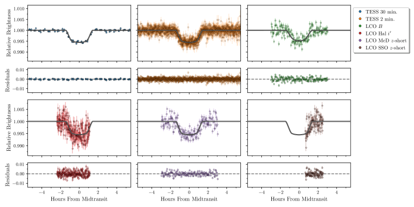
Figure 1: Photometry for TOI-1820. Our different photometric observations of TOI-1820 with the best-fitting transit model are shown with a grey line, and the residuals, following the subtraction of the best-fitting model, are shown below.

2 TESS photometry of candidate systems

The transiting planet candidates TOI-1820, TOI-2025, and TOI-2158 were identified by the Massachusetts Institute of Technology (MIT) Quick Look Pipeline (QLP; Huang et al. 2020) in a search of light curves extracted from the 30-minute cadence Full Frame Images (FFIs) using the box-least-squares (BLS; Kovács et al. 2002; Hartman & Bakos 2016) algorithm. Transit signals were detected for all three systems, which were then identified as TESS Objects of Interest (TOIs) by the TESS Science Office at MIT (Guerrero et al. 2021).

All three targets were subsequently put on the target list for 2-minute cadence. The 2-minute cadence data are processed by the Science Processing Operation Center (SPOC; Jenkins et al. 2016) team at the NASA Ames Research Center, where light curves are extracted through simple aperture photometry (SAP; Twicken et al. 2010; Morris et al. 2020) and processed using the Presearch Data Conditioning (PDC; Smith et al. 2012; Stumpe et al. 2012, 2014) algorithm.

We downloaded and extracted all the TESS light curves from the target pixel files using the lightkurve (Lightkurve Collaboration et al. 2018) package, where we use the implemented RegressionCorrector to correct for any background noise. We excluded cadences with severe quality issues. We also removed outliers. First we removed the transits from the light curve through a light-curve model using parameters from an initial fit. Next we applied a Savitsky-Golay filter and identified outliers through $5\sigma$ sigma clipping, which we then excluded from the unfiltered light curve with transits. For all three systems, we confirmed the presence of the transit-like features identified by QLP, by performing an independent search using the BLS and the Transit Least Squares (TLS; Hippke & Heller 2019) algorithm. We furthermore searched for additional transits, without finding hints of any.

2.1 TOI-1820

TOI-1820 was observed in Sector 22 (February 18, 2020 and March 18, 2020), with TESS’ camera 1 with a cadence of 30 minutes. TOI-1820 was identified on April 17, 2020 with a signal-to-noise ratio (S/N) of 53. TOI-1820 was observed again in Sector 49 (February 26, 2022 and March 26, 2022) with camera 1, this time with a cadence of 2 minutes. In the top left of Figure 1, we show the TESS light curve phase folded to the periodic transit signal occurring every 4.860674 d with a depth of $\sim$0.6%.

2.2 TOI-2025

TOI-2025 was observed with a 30-minute cadence using TESS’ camera 3 in Sector 14 (July 18, 2019 to August 15, 2019), Sectors 18-20 (November 2, 2019 to January 21, 2020), Sectors 24-26 (April 16, 2020 to July 4, 2020), as well as in 2-minute cadence in Sector 40 (June 24, 2021 to July 23, 2021) and Sector 47 (December 30, 2021 to January 28, 2022), also with camera 3. Since the TESS light curves of TOI-2025 display a periodic 8.872078 d dip of $\sim$0.7% with a S/N of 151, the candidate was announced as a TOI on June 19, 2020. The two panels on the top left of Figure 2 shows the phase-folded TESS light curves.

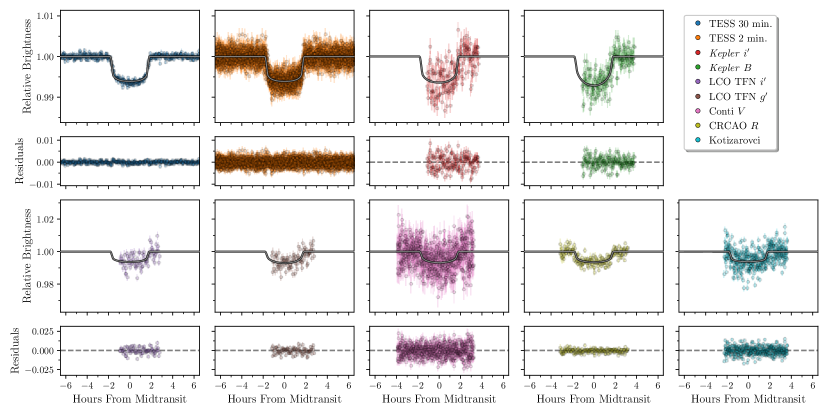
Figure 2: Photometry for TOI-2025. Our different photometric observations of TOI-2025 with the best-fitting transit model are shown with a grey line, and the residuals, following the subtraction of the best-fitting model, are shown below.

2.3 TOI-2158

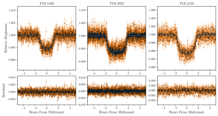
Figure 14: TESS curves. A close-up of the TESS 2-min (orange) and 30-min (blue) cadence light curves for TOI-1820 (left), TOI-2025 (middle), and TOI-2158 (right). The residuals show no structure around the transits.

TOI-2158 was observed with TESS’ camera 1 during Sector 26 (June 8, 2020 to July 4, 2020) with a cadence of 30 minutes, and in Sector 40 (June 24, 2021 to July 23, 2021) with a 2-minute cadence. On August 10, 2020, TOI-2158 was announced as a TOI with a S/N of 59. The TESS light curve for TOI-2158 can be seen in the top of Figure 3, phase folded onto the 8.60077 d signal showing the $\sim$0.5% decrease in flux. A close-up of the TESS light curves for all three systems can be found in Figure 14.

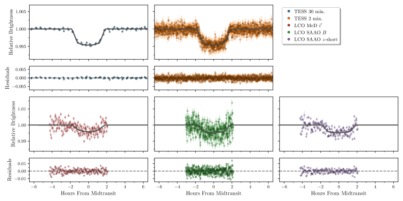
Figure 3: Photometry for TOI-2158. Our different photometric observations of TOI-2158 with the best-fitting transit model are shown with a grey line, and the residuals, following the subtraction of the best-fitting model, are shown below.

Table 1: Stellar parameters.

	TESS Object of Interest	TOI-1820	TOI-2025	TOI-2158
	TESS Input Catalogue	TIC 393831507	TIC 394050135	TIC 342642208
	TYCHO-2	TYC 1991-1863-1	TYC 4595-797-1	TYC 1577-691-1
$V$a	Tycho $V$ magnitude	10.90	11.60	10.89
$G$b	Gaia $G$ magnitude	10.97	11.36	10.67
$\alpha_{\mathrm{J2000}}$b	Right Ascension	12:30:44.813	18:51:10.861	18:27:14.413
$\delta_{\mathrm{J2000}}$b	Declination	27:27:07.206	82:14:43.492	20:31:36.793
$\mu_{\alpha}$b	Proper motion in R.A. (mas yr-1)	50.54$\pm$0.08	2.79$\pm$0.04	-44.00$\pm$0.04
$\mu_{\delta}$b	Proper motion in Dec. (mas yr-1)	-33.93$\pm$0.08	-4.52$\pm$0.05	7.89$\pm$0.07
$\varpi$b	Parallax (mas)	4.00$\pm$0.06	2.95$\pm$0.02	5.01$\pm$0.04
$\pi$b	Distance (pc)	250$\pm$4	339$\pm$2	200$\pm$1
$T_{\mathrm{eff}}$c	Effective temperature (K)	5734$\pm$50	5880$\pm$53	5673$\pm$50
$\log g$c	Surface gravity (dex)	4.24$\pm$0.05	4.17$\pm$0.06	4.19$\pm$0.05
$\rm[Fe/H]$c	Metallicity (dex)	0.14$\pm$0.15	0.18$\pm$0.08	0.47$\pm$0.08
$v\sin i_{\star}$c	Projected rotational velocity (km s-1)	4.5$\pm$0.8	6.0$\pm$0.3	3.7$\pm$0.5
$A_{\mathrm{V}}$d	Extinction (mag)	0.04$\pm$0.02	0.10$\pm$0.03	0.24$\pm$0.02
$F_{\mathrm{bol}}$c	Bolometric flux (erg s-1 cm-2)	$(1.017\pm 0.018)\times 10^{-9}$	$(7.02\pm 0.16)\times 10^{-10}$	$(1.540\pm 0.018)\times 10^{-9}$
$R_{\star}$d	Radius (R⊙)	1.51$\pm$0.06	1.56$\pm$0.03	1.41$\pm$0.03
$M_{\star}$d	Mass (M⊙)	1.04$\pm$0.13	1.32$\pm$0.14	1.12$\pm$0.12
$P_{\mathrm{rot}}/\sin i$d	Rotation period (days)	25$\pm$6	13.2$\pm$0.7	19$\pm$3
$P_{\mathrm{pred}}$d	Predicted rotation period (days)	40$\pm$2	-	43$\pm$3
$\log$ R${}^{\prime}_{\mathrm{HK}}$e	Activity	-5.37e	-	-5.06$\pm$0.05
$\tau$d	Age (Gyr)	11$\pm$2	1.7$\pm$0.2	8$\pm$1
$\rho$d	Density (g cm-3)	0.43$\pm$0.07	0.49$\pm$0.06	0.56$\pm$0.07

• Parameters of the stellar hosts in the three systems of this study.

• Tycho-2 (Høg et al. 2000).

• Gaia EDR3 (Gaia Collaboration et al. 2021).

• This work: SPC.

• This work: SED.

• This work: HIRES spectra.

3 Ground-based observations

In addition to TESS space-based photometry, we gathered ground-based photometry via the Las Cumbres Observatory Global Telescope (LOCGT; Brown et al. 2013), as well as ground-based spectroscopic measurements from different telescopes. Reconnaissance spectroscopy was acquired with the High Resolution Echelle Spectrometer (HIRES; Vogt et al. 1994) located at the Keck Observatory, the Tillinghast Reflector Echelle Spectrograph (TRES; Fűrész 2008) situated at the Fred L. Whipple Observatory, Mt. Hopkins, AZ, USA, as well as the FIber-fed Echelle Spectrograph (FIES; Frandsen & Lindberg 1999; Telting et al. 2014) at the Nordic Optical Telescope (NOT; Djupvik & Andersen 2010) of the Roque de los Muchachos observatory, La Palma, Spain.

To confirm and characterise the systems in terms of masses, bulk densities, and orbital parameters, we monitored the systems with the FIES spectrograph, and the Tull Coude Spectrograph (Tull et al. 1995) at the 2.7 m Harlan J. Smith telescope at the McDonald Observatory, Texas, USA. The FIES and Tull spectrographs are both cross-dispersed spectrographs with resolving powers of 67,000 (in high-resolution mode) and 60,000, respectively. Finally, to investigate companionship in the systems, we obtained speckle imaging using the 2.5-m reflector at the Caucasian Mountain Observatory of Sternberg Astronomical Institute (CMO SAI; Shatsky et al. 2020).

3.1 Speckle interferometry with SPP

TOI-2158, TOI-2025, and TOI-1820 were observed using speckle interferometry with the SPeckle Polarimeter (SPP; Safonov et al. 2017) on the 2.5-m telescope at the Sternberg Astronomical Institute of Lomonosov Moscow State University (SAI MSU). The detector has a pixel scale of 20.6 mas px^-1, and the angular resolution was 83 mas. The atmospheric dispersion compensation by two direct vision prisms allowed us to use the relatively broadband $I_{c}$ filter. For all targets, 4000 frames of 30 ms were obtained. The detection limits are provided in Figure 4. For TOI-2158 and TOI-2025, we did not detect any stellar companions, with limits for $\Delta$mag for any potential companion of 6.5 mag and 7 mag at $1^{\prime\prime}$, respectively.

3.1.1 Stellar companion to TOI-1820

For TOI-1820 we detected a companion 4.0 magnitudes fainter than the primary on December 2, 2020 and July 15, 2021. The separation, position angle, and contrast were determined by the approximation of the average power spectrum with the model of a binary star (see Eq. (9) in Safonov et al. 2017). As the weight for the approximation, we took the inverse squared uncertainty of the power spectrum determination. The results are presented in Table 2. All binarity parameters for the two dates coincide within the uncertainties. According to Gaia EDR3 (Gaia Collaboration et al. 2021), the proper motion of TOI-1820 is relatively high, being $50.54\pm 0.08$ mas yr^-1 and $-33.93\pm 0.08$ mas yr^-1 along right ascension and declination, respectively. If the companion of TOI-1820 were a background star, its position with respect to TOI-1820 would change by $37.694\pm 0.051$ mas between the two epochs of our observations. As long as we see a displacement much smaller than this, we conclude that TOI-1820 and its companion are gravitationally bound. With a Gaia parallax of 4 mas (see Table 1), we find a physical separation between the target and the companion of $\approx$110 AU. Furthermore, from our HIRES reconnaissance and using the algorithm from Kolbl et al. (2015), we can constrain this secondary companion to only contribute 1% in flux if the radial velocity (RV) separation between the components in TOI-1820 is greater than 10 km/s. If the RV separation were less than 10 km s^-1, the flux of the secondary would have been unconstrained without the speckle interferometry.

Table 2: Speckle observations of TOI-1820.

Date	Separation	P.A.	$\Delta m$
UT	mas	∘
2020-12-02	$470\pm 5$	$102.6\pm 0.3$	$4.0\pm 0.1$
2021-07-15	$474\pm 8$	$101.7\pm 0.9$	$3.7\pm 0.1$

• Results from the SPP speckle interferometry of TOI-1820: separation, position angle, and contrast.

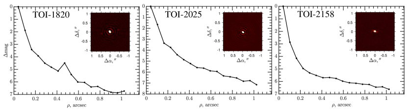
Figure 4: Speckle interferometry. SAI-2.5m speckle sensitivity curve and autocorrelation function (ACF) for TOI-1820 (left panel), TOI-2025 (middle panel), and TOI-2158 (right panel). All images shown here were taken in the $I$-band. Only the speckle image of TOI-1820 shows evidence of a nearby companion, as can be seen by the bump in the ACF around 0.45 arcsec.

3.2 Photometric follow-up

We acquired ground-based time-series follow-up photometry of TOI-1820, TOI-2025, and TOI-2158 as part of the TESS Follow-up Observing Program (TFOP; Collins 2019) to attempt to: (1) rule out or identify nearby eclipsing binaries (NEBs) as potential sources of the detection in the TESS data; (2) detect the transit-like events on target to confirm the depth, and thus the TESS photometric deblending factor; (3) refine the TESS ephemeris; and (4) place constraints on transit depth differences across optical filter bands. We used the TESS Transit Finder, which is a customised version of the Tapir software package (Jensen 2013), to schedule our transit observations. Unless otherwise noted, the images were calibrated and the photometric data were extracted using the AstroImageJ (AIJ) software package (Collins et al. 2017). The observing facilities are described below, and the individual observations are detailed in Table 4. The ground-based light curves for TOI-1820, TOI-2025, and TOI-2158 are shown in Figure 1, Figure 2, and Figure 3, respectively.

We observed six transits using the Las Cumbres Observatory Global Telescope (LCOGT; Brown et al. 2013) 1.0-m and 0.4-m networks. Three transits were observed in alternating filter mode, resulting in a total of nine light curves. The 1-m telescopes are equipped with $4096\times 4096$ pixel SINISTRO cameras having an image scale of $0\aas@@fstack{\prime\prime}389$ per pixel, resulting in a $26\arcmin\times 26\arcmin$ field of view. The 0.4-m telescopes are equipped with $2048\times 3072$ pixel SBIG STX6303 cameras having an image scale of 0$\aas@@fstack{\prime\prime}$57 pixel^-1, resulting in a $19\arcmin\times 29\arcmin$ field of view. The images were calibrated by the standard LCOGT BANZAI pipeline (McCully et al. 2018).

We observed a transit from KeplerCam on the 1.2-m telescope at the Fred Lawrence Whipple Observatory using alternating filters, resulting in two light curves. The $4096\times 4096$ Fairchild CCD 486 detector has an image scale of $0\aas@@fstack{\prime\prime}336$ per pixel, resulting in a $23\aas@@fstack{\prime}1\times 23\aas@@fstack{\prime}1$ field of view.

We observed one transit each from the Kotizarovci Private Observatory 0.3-m telescope near Viskovo, Croatia, the C.R. Chambliss Astronomical Observatory (CRCAO) 0.6-m telescope at Kutztown University near Kutztown, PA, and the Conti Private Observatory 0.3-m telescope near Annapolis, MD. The Kotizarovci telescope is equipped with a $765\times 510$ pixel SBIG ST7XME camera having an image scale of $1\aas@@fstack{\prime\prime}2$ per pixel, resulting in a $15\arcmin\times 10\arcmin$ field of view. The CRCAO telescope is equipped with a $3072\times 2048$ pixel SBIG STXL-6303E camera having an image scale of $0\aas@@fstack{\prime\prime}76$ after $2\times 2$ pixel image binning, resulting in a $13\arcmin\times 20\arcmin$ field of view. The Conti telescope is equipped with a $2750\times 2200$ pixel StarlightXpress SX694M camera having an image scale of $1\aas@@fstack{\prime\prime}0$ after $2\times 2$ pixel image binning, resulting in a $23\arcmin\times 18\arcmin$ field of view.

3.3 RV follow-up

Our NOT and McDonald Observatory monitoring was carried out from May 2020 to June 2022. In Table 5 and Table 6 we list all epochs and RVs for TOI-1820 and TOI-2025, respectively. Table 7 and Table 8 contain all epochs and RVs for and TOI-2158.

We reduced the FIES spectra using the methodology described in Buchhave et al. (2010) and Gandolfi et al. (2015), which includes bias subtraction, flat fielding, order tracing and extraction, and wavelength calibration. We traced the RV drift of the instrument acquiring long-exposed ThAr spectra ($\sim$80 s) immediately before and after each science observation. The science exposure time was set between1800-2700 seconds, depending on the sky conditions and scheduling constraints. As our exposures were longer than 1200 s, we split the exposure in three sub-exposures to remove cosmic ray hits using a sigma clipping algorithm while combining the frames. RVs were derived via multi-order cross-correlations, using the first stellar spectrum as a template.

For Tull we used 30-minute integrations to give a S/N of 60-70 per pixel. An $I_{2}$ gas absorption was used to provide the high-precision RV metric. All Tull spectra were reduced and extracted using standard IRAF tasks. Radial velocities were extracted using the Austral code (Endl et al. 2000).

To validate the planetary nature of the transiting signal in TOI-1820 and fully characterise the system, we acquired 18 spectra with FIES and 12 spectra with Tull, shown to the left in Figure 5. Figure 6 displays the generalised Lomb-Scargle (GLS; Lomb 1976; Scargle 1982) periodograms with TOI-1820 to the left, in which the $\sim$4.9 d transiting signal has been overplotted as the dashed line. This periodicity corresponds to the peak that we see in the GLS of the RVs.

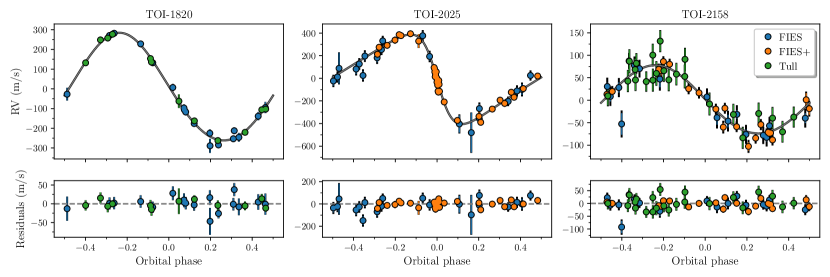
Figure 5: Radial velocities. From left to right are our FIES (blue), FIES+ (orange), and Tull (green) RVs for TOI-1820, TOI-2025, and TOI-2158, respectively, where the black parts of the error bars denote the jitter added in quadrature. The grey curves are the best-fitting models. In the bottom row are the residuals after subtracting the best-fitting models.

Figure 6: Generalised Lomb-Scargle periodograms. From left to right are the GLS periodograms for TOI-1820, TOI-2025, and TOI-2158. In the top row, we show the GLS periodograms directly from the RVs, and in the bottom we have removed the orbit of the planet. The vertical dashed lines from left to right denote the 4.9 d, 8.9 d, and 8.6 d signals seen in the photometry for TOI-1820, TOI-2025, and TOI-2158, respectively. The solid lines are our baselines, i.e. $1/(t_{\mathrm{last\ RV}}-t_{\mathrm{first\ RV}})$ with $t_{\mathrm{first\ RV}}$ and $t_{\mathrm{last\ RV}}$ being the times for the first and last acquired RVs. The horizontal solid, dot-dashed, and dashed lines show the 10%, 1%, and 0.1% false alarm probabilities, respectively.

We collected a total of 46 FIES RVs to validate the planetary nature of the signal, as well as to characterise the TOI-2025 system. In the middle panel of Figure 5, FIES+ refers to RVs collected after July 1, 2021 (see Section 5). As before, the transiting signal coincides with the peak in the GLS periodogram in the middle panels of Figure 6.

For TOI-2158 we collected 30 FIES RVs and 23 Tull RVs, shown in the right panel of Figure 5. As for the other two systems, the peak associated with the $\sim$8.6 d period planet is detected in the GLS periodogram in Figure 6, since it is stronger than the false alarm probability.

4 Stellar parameters

We made use of the stellar parameter classification (SPC; Buchhave et al. 2012, 2014; Bieryla et al. 2021) tool to obtain stellar parameters, where we reduced and extracted the spectra following the approach in Buchhave et al. (2010). For TOI-2025 and TOI-2158, we used the TRES spectra as reconnaissance, and for TOI-1820, we used our FIES spectra. The derived stellar parameters are tabulated in Table 1.

In addition, for TOI-1820 we also used our HIRES spectra with Specmatch-Synth to derive stellar parameters as described in Petigura et al. (2017). From the two HIRES spectra, we find $T_{\mathrm{eff}}=5695\pm 100$ K, $\log g=4.1\pm 0.1$, [Fe/H]$=0.01\pm 0.06$, and $v\sin i=3.07\pm 0.77$ km s^-1. We also estimated the R${}^{\prime}_{\mathrm{HK}}$ activity indicator. As a result we obtained $\log$R${}^{\prime}_{\mathrm{HK}}$ = -5.37, a hint that the star is inactive.

4.1 SED

As an independent check on the derived stellar parameters, we performed an analysis of the broadband spectral energy distribution (SED) together with the Gaia EDR3 (Gaia Collaboration et al. 2021) parallax in order to determine an empirical measurement of the stellar radius, following the procedures described in Stassun & Torres (2016); Stassun et al. (2017, 2018). In short, we pulled the $B_{T}V_{T}$ magnitudes from Tycho-2, the $BVgri$ magnitudes from APASS, the $JHK_{S}$ magnitudes from 2MASS, the W1–W4 magnitudes from WISE, and the $GG_{\rm BP}G_{\rm RP}$ magnitudes from Gaia. We also used the GALEX NUV flux when available. Together, the available photometry spans the stellar SED over the wavelength range 0.35–22 $\mu$m, and extends down to 0.2 $\mu$m when GALEX data are available (see Figure 7). We performed a fit using Kurucz stellar atmosphere models, with the priors on effective temperature ($T_{\rm eff}$), surface gravity ($\log g$), and metallicity ([Fe/H]) from the spectroscopically determined values. The remaining free parameter was the extinction ($A_{V}$), which we restricted to the maximum line-of-sight value from the dust maps of Schlegel et al. (1998).

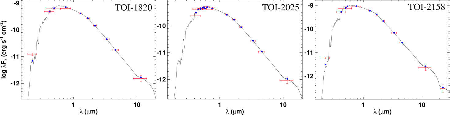
Figure 7: Spectral Energy Distribution. The SEDs for TOI-1820 (left panel), TOI-2025 (middle panel), and TOI-2158 (right panel). Red symbols represent the observed photometric measurements, where the horizontal bars represent the effective width of the passband. Blue symbols are the model fluxes from the best-fit Kurucz atmosphere model (black).

The resulting SED fits are shown in Figure 7 for TOI-1820, TOI-2025, and TOI-2158 with reduced $\chi^{2}$ values of 1.5, 1.2, and 1.2, respectively. The resulting best-fit are summarised in Table 1. Integrating the (unreddened) model SED gives the bolometric flux at Earth, $F_{\rm bol}$, which with the $T_{\rm eff}$ and the Gaia EDR3 parallax (with no systematic adjustment; see Stassun & Torres 2021) gives the stellar radius. The stellar mass can then be determined empirically from the stellar radius and the spectroscopic $\log g$, and compared to the mass estimated from the empirical relations of Torres et al. (2010). Finally, we can estimate the age of the star from the spectroscopic $R^{\prime}_{\rm HK}$ via the empirical relations of Mamajek & Hillenbrand (2008), which we can also corroborate by comparing the stellar rotation period predicted at that age from the empirical gyrochronology relations of Mamajek & Hillenbrand (2008) against that determined from the stellar radius together with the specroscopic $v\sin i$. These parameters are also summarised in Table 1. The rather old ages inferred for TOI-1820 and TOI-2158 would predict slow stellar rotation periods of $P_{\rm rot}=40\pm 2$ d and $P_{\rm rot}=43\pm 3$ d, respectively, whereas the (projected) rotational periods estimated from the spectroscopic $v\sin i$ together with $R_{\star}$ gives $P_{\rm rot}/\sin i=24.9\pm 6.3$ d and $P_{\rm rot}/\sin i=19.3\pm 3.2$ d, suggesting either somewhat younger ages, or a process that kept the stars rotating faster than expected for their ages.

It is interesting that both TOI-1820 and TOI-2158 appear to be rotating faster than what would be expected given their ages, especially seeing as both of these stars host a hot Jupiter. Discrepancy between ages inferred from isochrone fitting and gyrochronology among hot Jupiter hosts has been seen in studies by Brown (2014) and Maxted et al. (2015), and both studies suggested tidal spin-up as a possible explanation. Further evidence for this has recently been found in Tejada Arevalo et al. (2021). Tidal spin-up might, therefore, be the mechanism responsible for the discrepancy we are seeing in TOI-1820 and TOI-2158. Of course, this might also apply to the TOI-2025 system as this system also harbours a hot Jupiter, but as this system is younger, the effect might be less pronounced. We examined the residuals of the light curves from our best-fitting models (Figure 14) to see if we could see any signs of stellar variability, for instance, rotation. However, we did not detect any signals.

5 Joint analysis

To estimate the planetary and orbital parameters, we fit the photometry and the RVs jointly, where we extracted confidence intervals through Monte Carlo Markov chain (MCMC) sampling using the emcee package by Foreman-Mackey et al. (2013). We modelled the light curves using the batman package (Kreidberg et al. 2015), which utilises the formalism by Mandel & Agol (2002). To account for any morphological light curve distortion (Kipping 2010) caused by the 30-minute sampling, we oversampled our 30-minute-cadence light curves to correspond to a sampling of 2 minutes.

In an attempt to mitigate correlated noise in the TESS photometry, we made use of Gaussian process (GP) regression through the celerite package (Foreman-Mackey et al. 2017). We used the Matérn-3/2 kernel, which includes two hyper parameters: the amplitude of the noise, $A$, and the timescale, $\tau$. The only correction to the TESS data prior to the MCMC was the aforementioned background correction. For our ground-based photometry, we did not have long out-of-transit baselines. Therefore, we did not model the noise from these transits with GPs, instead we used a Savitsky-Golay filter to de-trend the data with each draw in our MCMC.

To fit the RVs we used a Keplerian orbit, where we naturally had different systemic velocities, $\gamma$, for the RVs stemming from FIES and Tull, when this is relevant. Due to a refurbishment of the FIES spectrograph, an offset in RV was introduced between the RVs obtained before July 1, 2021 and those obtained after. We assigned two independent systemic velocities and two independent jitter terms to RVs obtained before (FIES) and after (FIES+) this date.

Our MCMC analysis for the three systems stepped in $\cos i$ instead of $i$, as well as in $\sqrt{e}\cos\omega$ and $\sqrt{e}\sin\omega$ instead of $e$ and $\omega$. Furthermore, the code stepped in the sum of the limb darkening parameters, namely $q_{1}+q_{2}$, where we applied a Gaussian prior with a width of 0.1. We instead fixed the difference fixed, $q_{1}-q_{2}$, during the sampling. We retrieved the starting values of $q_{1}$ and $q_{2}$ for the TESS passband from the table Claret (2017), while we used the values from Claret et al. (2013) for the ground-based photometry. Furthermore, we used $V$ as a proxy for our transit observations of TOI-2025 using FIES. The initial and resulting values for the limb-darkening coefficients can be found in Table 10, Table 11, and Table 12.

We list all the adopted priors in Table 9, where a hyphen denotes that the associated parameter is not relevant for that run. We define our likelihood function as

$$\log\mathcal{L}=-0.5\sum_{i=1}^{N}\left[\frac{(O_{i}-C_{i})^{2}}{\sigma_{i}^{2}}+\log 2\pi\sigma_{i}^{2}\right]+\sum_{j=1}^{M}\log\mathcal{P}_{j}\,,$$ (1)

where $N$ indicates the total number of data points from photometry and RVs. $C_{i}$ represents the model corresponding to the observed data point $O_{i}$. $\sigma_{i}$ represents the uncertainty for the $i$th data point, where we add a jitter term in quadrature and a penalty in the likelihood for the RVs. $\mathcal{P}_{j}$ is the prior on the $j$th parameter.

We ran our MCMC until convergence, which we assessed by looking at the rank-normalised $\hat{R}$ diagnostic test as implemented in the rhat module in ArviZ (Kumar et al. 2019).

5.1 TOI-1820

Given the large separation of around 110 AU for the companion, the orbital period must be rather large and the expected $K$-amplitude must be rather small, meaning that, even if it is bound, it will not affect our RVs. The companion will, however, dilute the light curve. We therefore include a contaminating factor, where we write the total flux as a function of time as $F(t)=(F_{1}(t)+F_{2})/(F_{1}+F_{2})$ with $F_{1}(t)$ and $F_{1}$ being the flux respectively in- and out-of-transit from the planet hosting star, and $F_{2}$ is the (constant) flux from the contaminating source (or sources). Here, we included the flux from the contaminating source as a fraction of the host, $F_{2}/F_{1}$, as the difference in magnitude, namely $\delta\rm M=-2.5\log(F_{2}/F_{1})$. Conveniently, $\delta\rm M$ is derived from observations in the $I$-band, which is close to the bandpasses from TESS, $i^{\prime}$, and $z$-short (Figure 1). However, the dilution might be overestimated in the $B$-band. Therefore, we adopted a different value for the $B$-band of $\delta M=4.5\pm 1.0$ as the companion is most likely a cooler star.

5.2 TOI-2025

For TOI-2025, we have two sets of light curves with different cadences (2 min. and 30 min.), and we apply two different oversampling factors, while using the same limb darkening coefficients for both. We observed a spectroscopic transit of TOI-2025 at the NOT (FIES+) on the night starting on the August 8, 2021, allowing us to determine the projected obliquity, $\lambda$, of the host star. The RVs obtained during this transit night can be seen in Figure 8. We therefore also included a model for the Rossiter-McLaughlin (RM; Rossiter 1924; McLaughlin 1924) effect using the algorithm by Hirano et al. (2011) for this fit. We used our SPC value in Table 1 for $v\sin i_{\star}$ as a prior. For the macro- and micro-turbulence, we used priors stemming from the relations in Doyle et al. (2014) and Bruntt et al. (2010), respectively, along with the stellar parameters in Table 1.

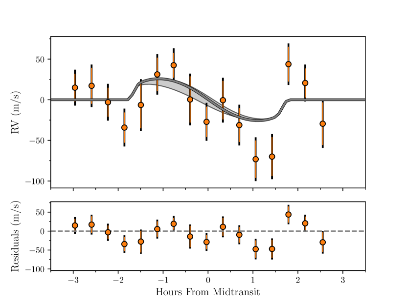
Figure 8: Rossiter-McLaughlin effect in TOI-2025. Our in-transit observations of TOI-2025 with FIES+. Top: The Keplerian orbit and quadratic trend has been subtracted from the RVs to better show the RM effect, with the grey line being the best-fitting model. The shaded area denotes the confidence interval in the projected obliquity, $\lambda=$$9^{+33}_{-31}$ ^∘. Bottom: Here we have further subtracted this best-fitting model from the RVs.

We carried out three MCMC runs for TOI-2025 to investigate the long-term trend: 1) a run where we included two additional parameters: a second order, $\ddot{\gamma}$, and a first-order acceleration parameter, $\dot{\gamma}$; 2) a run where we only included the first order parameter; and 3) a run where we did not allow for any long-term drift. These three runs are shown in Figure 9.

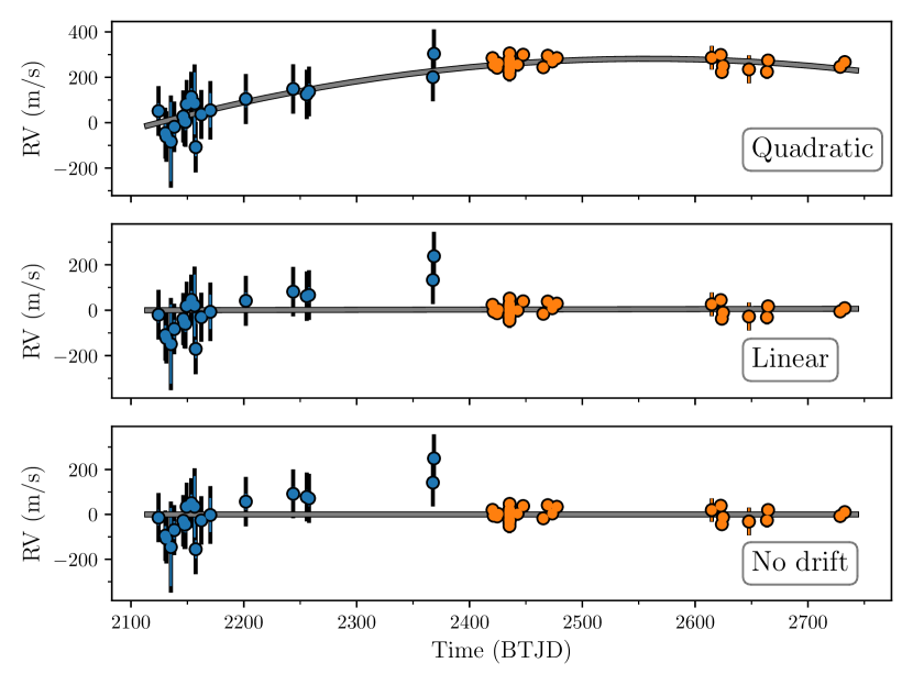
Figure 9: Long-term trend in TOI-2025. The symbols are the same as in Figure 5, but here the RVs are plotted against time, and we have subtracted the planetary signal. Top: A fit where we allow for a quadratic trend. Middle: A fit where we only allow for a linear trend. Bottom: Here we do not include any long-term drift.

5.3 TOI-2158

Similarly to the case of TOI-2025, the RVs of TOI-2158 show a long-term trend. We therefore performed the same three runs as for TOI-2025. These are shown in Figure 10.

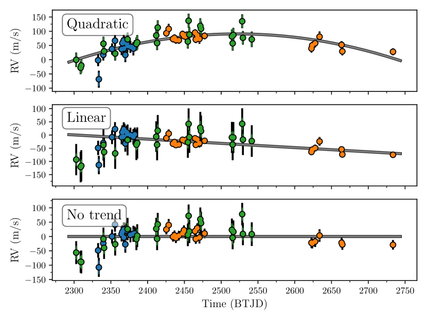
Figure 10: Long-term trend in TOI-2158. The symbols are the same as in Figure 5, but here the RVs are plotted against time, and we have subtracted the planetary signal. Top: A fit where we allow for a quadratic trend. Middle: Here we only allow for a linear trend. Bottom: Here we do not include any long-term drift.

6 Results

The results from the MCMC for our preferred orbital configuration for each of the systems are tabulated in Table 3. We find that TOI-1820b is a Jupiter-sized planet, $1.14\pm 0.02$ R_J, but significantly more massive, $2.3\pm 0.2$ M_J. With an orbital period of $4.860674\pm 0.000005$ d, it is the planet with the shortest orbital period in our sample. TOI-2025 has a similar size, $1.117\pm 0.009$ R_J, as TOI-1820, but has about twice its mass, $4.4\pm 0.3$ M_J. On the other end of the mass spectrum, we find TOI-2158 b with $0.82\pm 0.08$ M_J. TOI-2158 b is also a bit smaller than the two other planets with a radius of $0.960\pm 0.012$ R_J.

Table 3: Results from our MCMC analysis.

Parameter		TOI-1820	TOI-2025	TOI-2158
$P$	Period (days)	$4.860674\pm 0.000005$	$8.872078\pm 0.000007$	$8.60077\pm 0.00003$
$T_{0}$	Mid-transit time (BJD)	$2458903.0638\pm 0.0006$	$2458690.2898\pm 0.0004$	$2459018.9225_{-0.0011}^{+0.0010}$
$R_{\mathrm{p}}/R_{\star}$	Planet-to-star radius ratio	$0.0777\pm 0.0009$	$0.0736\pm 0.0004$	$0.0700\pm 0.0009$
$a/R_{\star}$	Semi-major axis to star radius ratio	$8.7\pm 0.3$	$12.7_{-0.4}^{+0.5}$	$11.4_{-0.5}^{+0.6}$
$K$	Velocity semi-amplitude (m s-1)	$273\pm 4$	$396\pm 10$	$75\pm 4$
$\cos i$	Cosine of inclination	$0.097\pm 0.005$	$0.023_{-0.023}^{+0.010}$	$0.075_{-0.006}^{+0.005}$
$\sqrt{e}\cos\omega$		$0.20\pm 0.02$	$-0.03_{-0.02}^{+0.03}$	$0.10_{-0.08}^{+0.10}$
$\sqrt{e}\sin\omega$		$0.031_{-0.031}^{+0.016}$	$0.643\pm 0.016$	$0.10_{-0.10}^{+0.05}$
$\gamma_{1}$	Systemic velocity FIES (m s-1)	$227_{-4}^{+5}$	$-383\pm 19$	$13\pm 9$
$\gamma_{2}$	Systemic velocity FIES+ (m s-1)	-	$-75_{-47}^{+45}$	$-23_{-15}^{+14}$
$\gamma_{3}$	Systemic velocity Tull (m s-1)	$13947\pm 4$	-	$-64794_{-13}^{+11}$
$\sigma_{1}$	Jitter FIES (m s-1)	$7_{-7}^{+3}$	$45_{-14}^{+12}$	$19_{-7}^{+5}$
$\sigma_{2}$	Jitter FIES+ (m s-1)	-	$19\pm 6$	$15_{-4}^{+3}$
$\sigma_{3}$	Jitter Tull (m s-1)	$5_{-5}^{+2}$	-	$12_{-11}^{+5}$
$\log A_{1}$	GP amplitude TESS 30 min.	$-6.98_{-0.10}^{+0.09}$	$-8.30\pm 0.06$	$-8.95_{-0.13}^{+0.12}$
$\log\tau_{1}$	GP timescale TESS 30 min. ($\log$ days)	$-0.77_{-0.14}^{+0.13}$	$-0.31_{-0.11}^{+0.10}$	$-1.7_{-0.4}^{+0.5}$
$\log A_{2}$	GP amplitude TESS 2 min.	$-7.36_{-0.11}^{+0.10}$	$-7.85_{-0.10}^{+0.09}$	$-7.271_{-0.016}^{+0.017}$
$\log\tau_{2}$	GP timescale TESS 2 min ($\log$ days)	$-1.03\pm 0.14$	$-0.23_{-0.14}^{+0.13}$	$-7.29_{-0.06}^{+0.07}$
$\ddot{\gamma}$a,b	Quadratic trend (m s-1 d-2)	-	$-0.0015\pm 0.0003$	$-0.0020\pm 0.0003$
$\dot{\gamma}$a,b	Linear trend (m s-1 d-1)	-	$1.4\pm 0.2$	$0.87_{-0.13}^{+0.14}$
$\delta\mathrm{M}_{I}$	Dilution $I$-band/TESS	$3.9_{-0.5}^{+0.4}$	-	-
$\delta\mathrm{M}_{B}$	Dilution $B$-band	$4.7_{-0.9}^{+0.8}$	-	-
$\lambda$	Projected obliquity (∘)	-	$9_{-31}^{+33}$	-
$v\sin i_{\star}$	Projected rotational velocity (km s-1)	-	$6.0\pm 0.3$	-
$\zeta$	Macro-turbulence (km s-1)	-	$4\pm 1$	-
$\xi$	Micro-turbulence (km s-1)	-	$1.3_{-0.9}^{+0.7}$	-
$e$	Eccentricity	$0.043\pm 0.008$	$0.41\pm 0.02$	$<0.070$ at $3\sigma$c
$\omega$	Argument of periastron (∘)	$9_{-9}^{+4}$	$93\pm 2$	$52_{-52}^{+19}$
$i$	Inclination (∘)	$84.4\pm 0.3$	$88.7_{-0.6}^{+1.3}$	$85.7_{-0.3}^{+0.4}$
$b$	Impact parameter	$0.840_{-0.013}^{+0.015}$	$0.29_{-0.29}^{+0.12}$	$0.86_{-0.03}^{+0.02}$
$T\rm_{4,1}$	Total transit duration (hours)	$2.92\pm 0.04$	$3.617_{-0.022}^{+0.017}$	$3.77_{-0.06}^{+0.05}$
$T\rm_{2,1}$	Time from 1st to 2nd contact (hours)	$0.61\pm 0.05$	$0.255_{-0.010}^{+0.009}$	$0.75\pm 0.07$
$R_{\mathrm{p}}$	Planet radius ($\rm R_{J}$)	$1.14\pm 0.02$	$1.117\pm 0.009$	$0.960\pm 0.012$
$M_{\mathrm{p}}$d	Planet mass ($\rm M_{J}$)	$2.3\pm 0.2$	$4.4\pm 0.3$	$0.82\pm 0.08$
$\rho_{\mathrm{p}}$	Planet density (g cm-3)	$2.0\pm 0.2$	$3.9\pm 0.3$	$1.14\pm 0.12$
$T_{\mathrm{eq}}$e	Equilibrium temperature (K)c	$1375\pm 12$	$1167\pm 11$	$1188\pm 10$
$a$	Semi-major axis (AU)	$0.061\pm 0.003$	$0.092\pm 0.004$	$0.075\pm 0.004$

• The parameters above the dashed line are the stepping parameters, and below are the derived parameters. The value given is the median and the uncertainty is the highest posterior density at a confidence level of 0.68.

• Zero-point for TOI-2158 is 2459302.92570 BJD_TDB.

• Zero-point for TOI-2025 is 2459124.41436 BJD_TDB.

• Two-sided $1\sigma$ distribution $e=0.031_{-0.031}^{+0.013}$.

• Calculated from Equation (2).

• Following Kempton et al. (2018).

For TOI-2025 and TOI-2158, we found evidence for long-term RV trends, as can be seen in Figure 9 and Figure 10. In both we also saw evidence for a curvature in the RVs, which we model with a quadratic term. There is no significant evidence for long-term RV changes in TOI-1820.

Assuming the long-term RV changes are due to further-out companions, we can glimpse information about their masses from some back-of-the-envelope calculations. We can therefore obtain an order of magnitude estimate for the periods of the outer companions as $P=-2\ddot{\gamma}/\dot{\gamma}$, resulting in periods of around 1870 d and 650 d for TOI-2025 and TOI-2158, respectively. Using the relation $K=\ddot{\gamma}P^{2}/4\pi^{2}$ derived in Kipping et al. (2011) with

$$\frac{M_{\rm p}\sin i}{\mathrm{M}_{\rm J}}=\frac{K\sqrt{1-e^{2}}}{28.4\leavevmode\nobreak\ \mathrm{m}\leavevmode\nobreak\ \mathrm{s}^{-1}}\left(\frac{P}{1\leavevmode\nobreak\ \mathrm{yr}}\right)^{1/3}\left(\frac{M_{\star}}{\mathrm{M}_{\odot}}\right)^{2/3}\,,$$ (2)

we can get an estimate of the masses of the companions. From this we get masses of $\approx 70$ M_J and $\approx 15$ M_J for the companions in TOI-2025 and TOI-2158, respectively.

6.1 The eccentricities of TOI-2025 b and TOI-1820 b

We find TOI-2025 b to travel on an eccentric orbit, $0.41\pm 0.02$. However, the argument of periastron is close to and fully consistent with $90^{\circ}$. This configuration can be deceptive when it comes to determining the eccentricity (e.g. Laughlin et al. 2005). This is because the RV curves would be symmetric for values close to $|\omega|=90$ ^∘, even for eccentric orbits.

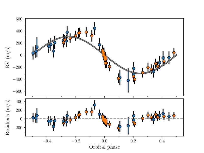
Figure 15: Circular solution for TOI-2025 b. Symbols are the same as in the middle panel of Figure 5, but here we have fixed $e=0$ during the MCMC.

To further investigate the orbital eccentricity, we carried out a few experiments. First, as mentioned, we ran an MCMC where we fixed $e$ to 0. The best-fitting model from this run can be seen in Figure 15, where the residuals clearly have structure in them. Our model involving a circular orbit does apparently not capture all the complexity present in the data. Consequently, the derived RV jitter terms for both FIES and FIES+ are significantly higher, with values of $111^{+18}_{-22}$ m s^-1 and $82^{+10}_{-13}$ m s^-1, respectively, as opposed to the values of $45^{+12}_{-14}$ m s^-1 and $19\pm 6$ m s^-1 from the eccentric fit. As we find a modest eccentricity for TOI-1820, we carried out a similar run for TOI-1820, finding marginally higher jitter (a couple of m s^-1) for the $e=0$ case.

As there might be stellar signals that are coherent on timescales of hours, but not days, and given that we have a much higher sampling during the transit night, it is worthwhile investigating if the eccentricity hinges on those measurements and to what extent. Therefore, we performed a fit in which the eccentricity was allowed to vary, but where we only included the first and the last data point from the transit night. Here, we obviously did not try to fit the obliquity. From this we get values of $e=0.42\pm 0.02$ and $\omega=91\pm 3$ ^∘, consistent with the values from the run using all the RV data.

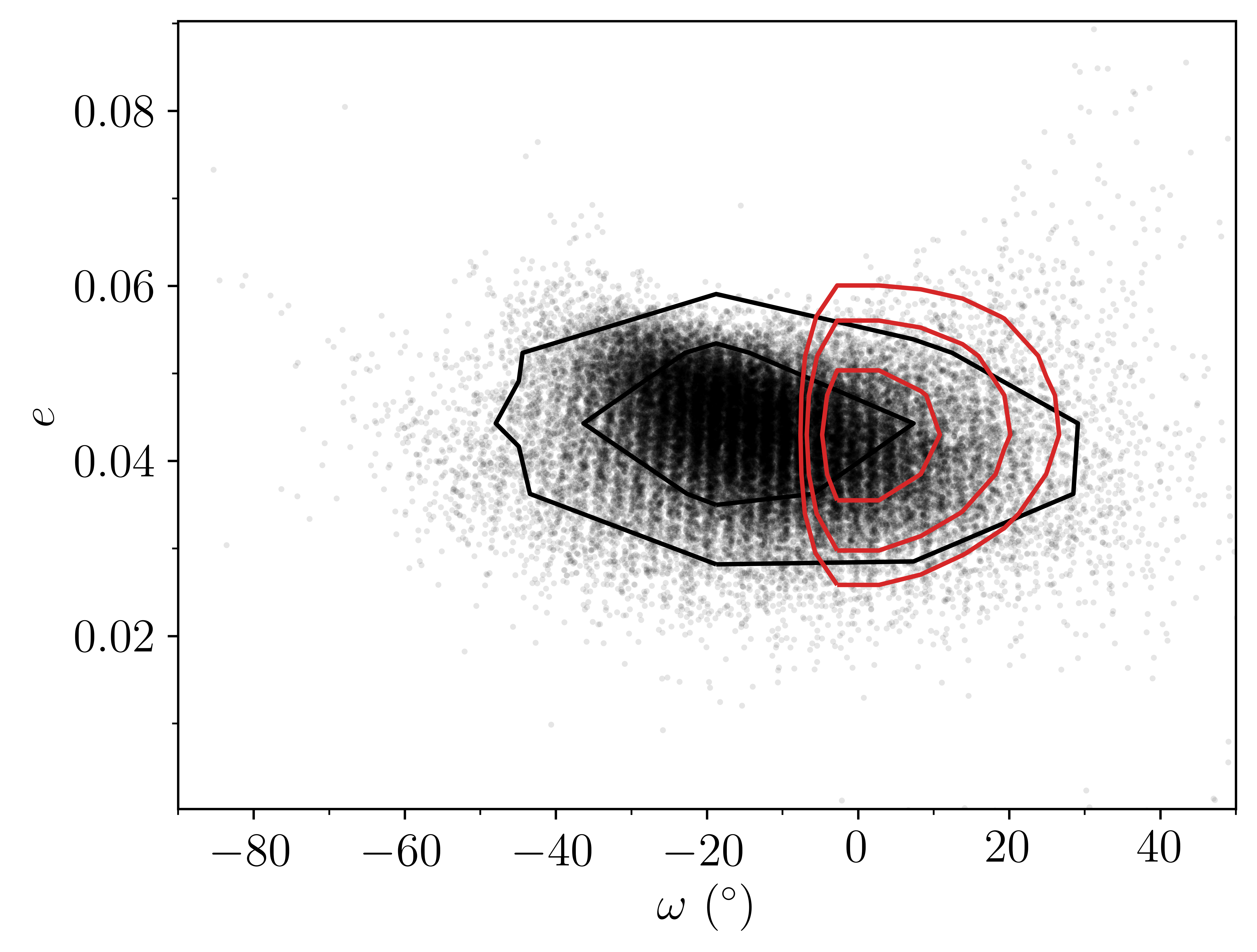
Figure 12: Bootstrapping the orbit of TOI-1820 b. Same as in Figure 11, but for TOI-1820 b.

Next we performed a bootstrap experiment using the RV data only. In our bootstrap we used alternate realisations of the data in Table 6, again excluding all but the first and last data point from the transit night. After redrawing a data set from the original data, we fit for $e$, $\omega$, $\gamma_{\mathrm{FIES}}$, $\gamma_{\mathrm{FIES+}}$, $K$, $\dot{\gamma}$, and $\ddot{\gamma}$. In Figure 11 we plot the results for $e$ and $\omega$ for the 50,000 realisations. Evidently, we recover an eccentric orbit even when we leave out certain data points. Therefore, we conclude that our result for the eccentricity is significant and does not hinge on a few data points. Again, we did a similar exercise for TOI-1820, which also yielded consistent results with the run from the MCMC, as seen in Figure 12. We thus conclude that the eccentricities for TOI-2025 b and TOI-1820 b are significant (at a confidence level of $20\sigma$ and $5\sigma$, respectively), while TOI-2158 b is consistent with a circular orbit.

6.2 The obliquity of TOI-2025

In addition to finding an eccentric orbit for the planet, we also measured the projected obliquity of TOI-2025. We find the projected obliquity to be consistent with no misalignment, $\lambda=$$9^{+33}_{-31}$ ^∘. The relevant transit RVs and our best-fitting model can be seen in Figure 8. Despite having only measured the projected obliquity, $\lambda$, here, we can make a strong argument that it is close to the obliquity, $\psi$, which requires the stellar inclination along the line of sight to be close to $90^{\circ}$. That $i_{\star}$ is close to $90^{\circ}$ is supported by Figure 3 in Louden et al. (2021), where a correlation between $T_{\mathrm{eff}}$ and $v\sin i_{\star}$ is plotted. From this plot we should not expect $v\sin i_{\star}$ to be markedly different from the value of $6.0\pm 0.3$ km s^-1 given the effective temperature for TOI-2025 of $\sim 5900$ K that we have found. This therefore suggests that the system is aligned.

7 Discussion and conclusions

We validated and characterised three hot Jupiters discovered by TESS: TOI-1820 b, TOI-2025 b, and TOI-2158 b. A commonality for all three systems is that we, in some way or another, see evidence for companions. The outer companions may have played a role in the migration of the gas giants, thus shaping the final architecture of the systems. Ngo et al. (2016) argue that sites hosting outer stellar companions are either more favourable environments for gas giant formation at all separations, or the presence of stellar companions might drive the inwards migration, such as through Kozai-Lidov (Kozai 1962; Lidov 1962), or other dynamical processes. Through our speckle interferometry of TOI-1820, we detected a $\sim$4 mag fainter stellar companion at a distance of $\sim$110 AU from the bright host. It would be interesting to obtain good estimates of the stellar parameters for this companion in order to assess whether it would have been able to drive Kozai-Lidov cycles responsible for the migration.

If the outer companions are planets within $\sim$1 AU from the stellar host, Becker et al. (2017) found that they should be coplanar with the inner hot Jupiters, suggesting that Kozai-Lidov migration would not be viable. However, if these companions are found at greater distances (gas giants $\gtrsim$5 AU or stellar $\gtrsim$100 AU), they could still be inclined and the formation of the hot Jupiter could take place through Kozai-Lidov migration (Lai et al. 2018). In the RVs for both TOI-2025 and TOI-2158, we see long-term quadratic trends. In contrast to TOI-1820, the companions in TOI-2025 and TOI-2158 might be of planetary, or at least substellar, nature and closer in (cf. the mass and period estimates in Section 6). As the companions in TOI-2025 and TOI-2158 are most likely found beyond 1 AU, given the (lower) estimates for their periods and the stellar masses, Kozai-Lidov migration could be a viable transport mechanism for TOI-2025 b and TOI-2158 b. TESS might be able to shed more light on these outer companions as more sectors become available. According to the Web TESS Viewing Tool, TOI-2025 should be observed again in Sectors 52, 53, and 58-60, and TOI-2158 is set to be observed in Sector 53. In addition, continued RV monitoring will help constrain the periods and masses.

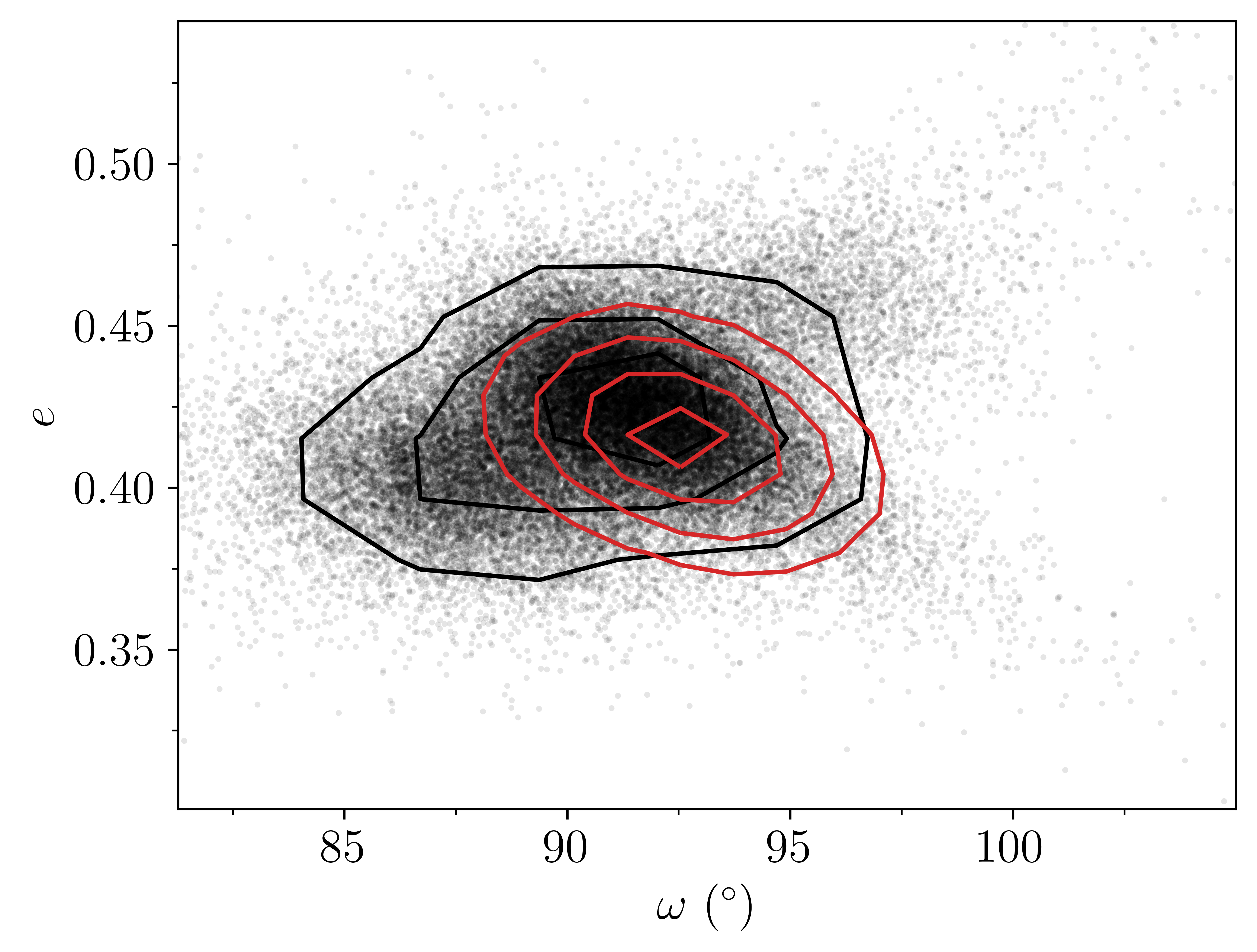
Figure 11: Bootstrapping the orbit of TOI-2025 b. A 2D histogram of our bootstrap with 50,000 iterations displaying the eccentricity plotted against the argument of periastron. Each point is one iteration and the black contours denote the confidence levels. The red contours are the posteriors from our MCMC tabulated in Table 3.

In Figure 13 we show the tidal diagram (left) and modified tidal diagram (right) from Bonomo et al. (2017a) with our measurements for TOI-1820 b, TOI-2025 b, and TOI-2158 b. We find that the orbital eccentricity of TOI-2158 b is consistent with $e=0$. This planet joins the small group of planets in Bonomo et al. (2017a) with circular orbits and relatively large values for $a/a_{\rm R}$, $a_{\rm R}$ being the Roche limit. This would allude to disc migration. However, given the age of $8\pm 1$ Gyr for TOI-2158, the orbit of the planet might have had sufficient time to circularise, should the migration have taken place through high-eccentricity migration. For TOI-1820 b we find a modest eccentricity of $0.043\pm 0.008$ (about three times that of Earth). In Figure 13 the planets with modest eccentricities are found at various relative masses and various relative distances. From the modified tidal diagram, it appears that TOI-1820 b should have a circularisation timescale of around 1-2 Gyr, and with the age of $11\pm 2$ Gyr for TOI-1820, this leaves plenty of time for the system to dampen the eccentricity in the case of high-eccentricity migration. However, this modest eccentricity is not irreconcilable with disc migration (Dawson & Johnson 2018). In contrast, TOI-2025 b belongs to the subgroup of systems with significant eccentricity. The planet TOI-2025 b is too massive for the star to effectively raise tides on the planet in order to circularise the orbit, meaning that the circularisation timescale is too long for the orbit to have been circularised (Dawson & Johnson 2018). The modified tidal diagram suggests that the circularisation timescale could be some $10$ Gyr, which is much longer than the age of $1.7\pm 0.2$ Gyr for this system.

On the same token, the planet seems to be massive enough for it to effectively raise tides on the star, while the star is sufficiently cool for tidal dissipation to be efficient (Winn et al. 2010; Albrecht et al. 2012). The projected obliquity we find for TOI-2025 is in line with other massive planets on eccentric, aligned orbits, such as HD 147506b (Winn et al. 2007), HD 17156 b (Narita et al. 2009), and HAT-P-34 b (Albrecht et al. 2012). Contrary to these findings, Rice et al. (2022) has found that cool stars ($T_{\mathrm{eff}}<$6100 K) harbouring eccentric planets tend to have higher obliquities. Although, due to the sample size it is still unclear whether misalignment is associated with orbital eccentricity. Given the orbital, stellar, and planetary parameters, the low projected obliquity in TOI-2025 might be the result of tidal alignment (Albrecht et al. 2022). If so it would be interesting to further reduce the uncertainty of the obliquity measurement to test if the system is aligned to within $1^{\circ}$ as recently observed in some systems (Albrecht et al. 2022). This would suggest tidal alignment, as primordial alignment would presumably lead to a certain spread, as it has apparently done in the Solar System. TOI-1820 and TOI-2158 would, for similar reasons, be excellent RM targets as well. In addition, their higher impact parameters might lead to an even higher accuracy.

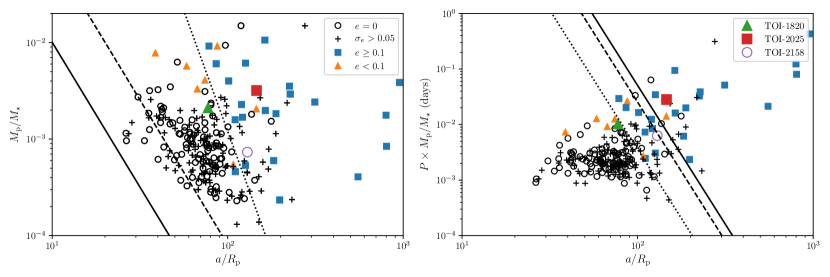
Figure 13: Tidal diagrams. Tidal diagrams for transiting giant planets from Bonomo et al. (2017a). Open circles denote planets on circular orbits with $\sigma_{e}<0.05$. Markers shown with pluses are planets with undertermined eccentrities, i.e. $\sigma_{e}>0.05$. Most of these are consistent with $e=0$. Triangles represent planets with significant, but small eccentricities $e<0.1$, and squares are eccentric systems $\geq 0.1$. Adhering to this notation we have shown the planets in our sample with the corresponding marker. However, we have colour coded them for clarity. Created from the catalogue Bonomo et al. (2017b). Left: Tidal diagram. The solid and dashed lines show the position of a planet with a separation of $a=a_{\mathrm{R}}$ and $a=2a_{\mathrm{R}}$, respectively ($a_{\mathrm{R}}$ being the Roche limit), and radius $R_{\mathrm{p}}=1.2$ R_J. The dotted line is a circularisation isochrone for a planet with $P=3$ d, $Q^{\prime}_{\mathrm{p}}=10^{6}$, and $e=0$. It should be noted that Eq. (1) in Bonomo et al. (2017a) used to create the dotted line should have $\pi$ in the numerator instead of the denominator (A. S. Bonomo private communication)

. Right: Modified tidal diagram. The dotted, dashed, and solid lines denote the 1, 7, and 14 Gyr circularisation timescales, respectively, assuming $e=0$ and $Q^{\prime}_{\mathrm{p}}=10^{6}$.

8 Acknowledgements

The authors would like to thank the referee, Louise D. Nielsen, for an insightful and helpful review of this work. The authors would also like to thank the staff at the Nordic Optical Telescope for their help and expertise. This paper includes data taken at the Nordic Optical Telescope under the programs IDs 59-210, 59-503, 61-510, 61-804, 62-506, and 63-505. This study is based on observations made with the Nordic Optical Telescope, owned in collaboration by the University of Turku and Aarhus University, and operated jointly by Aarhus University, the University of Turku and the University of Oslo, representing Denmark, Finland, and Norway, the University of Iceland and Stockholm University at the Observatorio del Roque de los Muchachos, La Palma, Spain, of the Instituto de Astrofisica de Canarias. This paper includes data taken at The McDonald Observatory of The University of Texas at Austin. This is University of Texas Center for Planetary Systems Habitability contribution #0053. We acknowledge the use of public TESS data from pipelines at the TESS Science Office and at the TESS Science Processing Operations Center. Resources supporting this work were provided by the NASA High-End Computing (HEC) programme through the NASA Advanced Supercomputing (NAS) Division at Ames Research Center for the production of the SPOC data products. Funding for the Stellar Astrophysics Centre is provided by The Danish National Research Foundation (Grant agreement no.: DNRF106). A.A.B., B.S.S., and I.A.S. acknowledge the support of Ministry of Science and Higher Education of the Russian Federation under the grant 075-15-2020-780(N13.1902.21.0039). The numerical results presented in this work were obtained at the Centre for Scientific Computing, Aarhus http://phys.au.dk/forskning/cscaa/. This work makes use of observations from the LCOGT network. Part of the LCOGT telescope time was granted by NOIRLab through the Mid-Scale Innovations Program (MSIP). MSIP is funded by NSF. P. R. and L. M. acknowledge support from National Science Foundation grant No. 1952545. This research made use of Astropy, a community-developed core Python package for Astronomy (Astropy Collaboration et al. 2013, 2018). This research made use of matplotlib (Hunter 2007). This research made use of TESScut (Brasseur et al. 2019). This research made use of astroplan (Morris et al. 2018). This research made use of SciPy (Virtanen et al. 2020). This research made use of corner (Foreman-Mackey 2016).

Appendix A Tables for RVs, priors, and limb-darkening coefficients

Table 4: Ground-based photometry.

Observatory	Aperture (m)	Location	UTC Date	Filter	Coverage	Planet
LCOGT1-Hal	0.4	Haleakala, HI, USA	2020-05-06	Sloan $i^{\prime}$	Ingress	TOI-1820 b
LCOGT-SSO	1.0	Siding Spring, Australia	2020-05-11	$z$-short2	Egress	TOI-1820 b
LCOGT-McD	1.0	McDonald Observatory, TX, USA	2021-02-12	$B$	Full	TOI-1820 b
LCOGT-McD	1.0	McDonald Observatory, TX, USA	2021-02-12	$z$-short	Full	TOI-1820 b
Kotizarovci	0.3	Viskovo, Croatia	2020-06-26	Baader $R$3	Full	TOI-2025 b
LCOGT-TFN	0.4	Tenerife, Canary Islands	2020-06-26	Sloan $g^{\prime}$	Egress	TOI-2025 b
LCOGT-TFN	0.4	Tenerife, Canary Islands	2020-06-26	Sloan $i^{\prime}$	Egress	TOI-2025 b
FLWO4-KeplerCam	1.2	Amado, Arizona, USA	2021-05-12	$B$	Egress	TOI-2025 b
FLWO-KeplerCam	1.2	Amado, Arizona, USA	2021-05-12	Sloan $i^{\prime}$	Egress	TOI-2025 b
CRCAO-KU	0.6	Kutztown, PA, USA	2021-05-21	$R$	Full	TOI-2025 b
Conti Private Obs.	0.3	Annapolis, MD, USA	2021-12-19	$V$	Full	TOI-2025 b
LCOGT-McD	0.4	McDonald Observatory, TX, USA	2020-08-06	Sloan $i^{\prime}$	Full	TOI-2158 b
LCOGT-SAAO	1.0	Cape Town, South Africa	2021-06-05	$B$	Full	TOI-2158 b
LCOGT-SAAO	1.0	Cape Town, South Africa	2021-06-05	$z$-short	Full	TOI-2158 b

• Information on our ground-based photometric observations.

• Las Cumbres Observatory Global Telescope (Brown et al. 2013).

• Pan-STARRS $z$-short.

• Baader $R$ longpass 610 nm.

• Fred L. Whipple Observatory.

Table 5: Radial velocities for TOI-1820.

Epoch (BJDTDB)	RV (m s-1)	$\sigma$ (m s-1)	Instrument
2459269.780732	13841.9	12.6	Tull
2459270.880079	14196.4	14.9	Tull
2459275.91069	14205.8	15.7	Tull
2459276.9072	14101.6	14.6	Tull
2459277.930989	13785.6	10.4	Tull
2459280.881956	14225.0	8.8	Tull
2459281.790658	14083.9	16.3	Tull
2459293.694114	13727.5	11.3	Tull
2459294.83763	14080.0	13.3	Tull
2459301.873852	13885.5	34.0	Tull
2459302.781944	13685.8	13.0	Tull
2459308.757963	13845.4	9.8	Tull
2458991.51119436	-0.0	18.9	FIES
2459204.77744922	128.2	16.8	FIES
2459206.67557103	130.2	27.7	FIES
2459215.77997042	-20.9	21.5	FIES
2459229.68962246	-63.7	35.2	FIES
2459233.68191458	231.9	17.5	FIES
2459235.67276872	86.3	19.8	FIES
2459239.60737547	-59.5	11.8	FIES
2459243.67146977	119.2	12.1	FIES
2459254.55706331	12.6	16.4	FIES
2459276.67782068	453.3	15.7	FIES
2459277.72833782	107.7	15.7	FIES
2459283.69993517	-28.2	15.6	FIES
2459284.68431354	198.0	31.6	FIES
2459285.67225885	495.6	15.3	FIES
2459290.64256983	507.0	15.5	FIES
2459291.542424	357.2	14.0	FIES
2459292.50793658	48.9	14.6	FIES

• The epoch, RVs, and errors from our RV monitoring of TOI-1820.

Table 6: Radial velocities for TOI-2025.

Epoch (BJDTDB)	RV (m s-1)	$\sigma$ (m s-1)	Instrument
2459124.41436227	2.5	33.9	FIES
2459130.45161579	-284.4	42.3	FIES
2459131.34610963	-183.9	38.9	FIES
2459135.35261256	-840.4	174.3	FIES
2459138.35644793	-379.9	39.6	FIES
2459146.37902542	-444.9	47.7	FIES
2459147.40383093	-333.3	32.7	FIES
2459148.33080998	-216.8	36.1	FIES
2459149.32822725	-11.5	24.1	FIES
2459153.43955164	-605.2	38.3	FIES
2459156.34166702	-245.9	136.3	FIES
2459157.36143997	-307.9	39.7	FIES
2459162.3066763	-682.9	29.3	FIES
2459170.33208575	-721.1	75.6	FIES
2459201.80136496	-85.7	36.0	FIES
2459243.76155035	-351.8	32.2	FIES
2459255.74010029	25.2	31.6	FIES
2459257.78775181	-33.9	34.1	FIES
2459367.59501228	-350.7	20.3	FIES
2459368.54449905	-121.1	25.9	FIES
2459420.48398551	2.2	17.3	FIES+
2459421.4708797	104.9	25.5	FIES+
2459424.55064799	488.6	17.1	FIES+
2459425.54286536	591.6	21.2	FIES+
2459442.62870736	541.1	27.8	FIES+
2459447.57636978	82.3	19.3	FIES+
2459465.4399404	43.1	14.5	FIES+
2459469.42183232	597.7	23.0	FIES+
2459473.38320428	-59.0	18.8	FIES+
2459477.44240997	488.6	17.6	FIES+
2459435.4210958	296.7	17.1	FIES+
2459435.43653977	288.1	22.1	FIES+
2459435.45173373	257.1	17.8	FIES+
2459435.46695905	215.0	18.6	FIES+
2459435.48219576	231.8	28.6	FIES+
2459435.49740642	258.4	20.6	FIES+
2459435.51261722	258.6	15.3	FIES+
2459435.52786928	205.3	28.5	FIES+
2459435.54310052	166.6	18.7	FIES+
2459435.5582903	182.1	23.7	FIES+
2459435.57347547	140.3	20.8	FIES+
2459435.58863805	87.2	23.0	FIES+
2459435.60382369	79.3	24.0	FIES+
2459435.61903594	182.0	21.4	FIES+
2459435.63457285	147.6	17.9	FIES+
2459435.65079739	85.8	26.2	FIES+
2459614.77148284	-118.2	50.0	FIES+
2459622.72491642	-155.3	17.7	FIES+
2459623.7179694	-171.9	24.4	FIES+
2459624.73548358	-5.4	17.8	FIES+
2459647.6942654	540.3	59.7	FIES+
2459663.68611219	419.4	27.8	FIES+
2459664.68704606	583.9	20.3	FIES+
2459728.62936384	-29.3	9.6	FIES+
2459732.6047247	197.9	14.3	FIES+

• The epoch, RVs, and errors from our RV monitoring of TOI-2025.

Table 7: FIES radial velocities for TOI-2158.

Epoch (BJDTDB)	RV (m s-1)	$\sigma$ (m s-1)	Instrument
2459332.67780456	0.1	10.5	FIES
2459333.70360452	-12.1	23.8	FIES
2459339.681805	-37.9	8.7	FIES
2459351.64286508	123.2	7.8	FIES
2459355.66056274	24.0	9.2	FIES
2459364.63370853	-15.1	10.9	FIES
2459365.60471439	4.7	7.2	FIES
2459367.51570125	93.2	8.1	FIES
2459367.64102824	71.2	11.0	FIES
2459368.63519994	140.6	8.4	FIES
2459369.68467584	111.0	18.1	FIES
2459371.62623245	72.3	5.9	FIES
2459372.49619057	19.1	14.2	FIES
2459376.59299817	96.0	11.3	FIES
2459380.64168281	31.2	15.6	FIES
2459382.55110354	-7.0	6.8	FIES
2459425.45350272	-0.0	5.1	FIES+
2459428.61860581	142.7	13.8	FIES+
2459434.45668389	-15.6	4.6	FIES+
2459436.5266032	77.5	4.6	FIES+
2459438.44453163	127.4	5.7	FIES+
2459442.44074223	-24.5	5.3	FIES+
2459447.49151578	141.4	4.7	FIES+
2459449.40026218	42.0	4.7	FIES+
2459451.55658931	-8.9	5.2	FIES+
2459453.507784	76.1	3.9	FIES+
2459464.43808474	151.5	4.2	FIES+
2459465.48015278	91.3	5.2	FIES+
2459467.45855826	7.2	4.3	FIES+
2459470.45543094	47.9	13.4	FIES+
2459477.40400508	-5.7	4.8	FIES+
2459622.7602177	-50.6	9.1	FIES+
2459623.75257858	-36.6	5.7	FIES+
2459627.76305009	115.6	10.1	FIES+
2459633.74209536	48.6	14.6	FIES+
2459663.7250026	49.6	6.4	FIES+
2459664.72649871	-27.3	8.8	FIES+
2459733.59894098	-31.8	4.9	FIES+

• The epoch, RVs, and errors from our FIES RV monitoring of TOI-2158.

Table 8: Tull radial velocities for TOI-2158.

Epoch (BJDTDB)	RV (m s-1)	$\sigma$ (m s-1)	Instrument
2459302.925697	-64804.4	23.8	Tull
2459308.916426	-64749.6	20.7	Tull
2459309.847096	-64745.0	23.6	Tull
2459339.927982	-64807.7	22.9	Tull
2459340.803182	-64804.8	21.5	Tull
2459355.902204	-64841.0	22.7	Tull
2459372.717338	-64779.2	22.0	Tull
2459384.739579	-64731.2	21.2	Tull
2459385.864151	-64672.0	23.6	Tull
2459411.718672	-64646.1	20.9	Tull
2459412.852352	-64662.1	23.1	Tull
2459413.7245	-64636.3	23.7	Tull
2459454.684757	-64668.7	22.9	Tull
2459455.705819	-64582.0	22.9	Tull
2459456.718945	-64660.5	24.8	Tull
2459471.635406	-64623.3	25.2	Tull
2459472.60132	-64609.5	23.6	Tull
2459514.575615	-64662.9	22.8	Tull
2459515.606634	-64660.8	23.8	Tull
2459516.580362	-64647.4	23.2	Tull
2459528.573076	-64735.0	22.6	Tull
2459529.557203	-64775.8	22.2	Tull
2459541.556578	-64646.5	25.7	Tull
2459610.026931	-64665.1	29.2	Tull
2459611.019771	-64694.2	26.6	Tull
2459622.022527	-64851.4	24.6	Tull
2459634.984303	-64685.8	27.5	Tull
2459692.973827	-64845.7	24.9	Tull
2459693.918368	-64826.4	22.2	Tull
2459705.915839	-64728.1	19.6	Tull
2459706.844475	-64782.3	20.9	Tull
2459707.907303	-64839.9	23.4	Tull
2459707.922283	-64835.6	23.7	Tull

• The epoch, RVs, and errors from our Tull RV monitoring of TOI-2158.

Table 9: Priors used in our MCMC.

Parameter	TOI-1820	TOI-2025	TOI-2158
$P$	$\mathcal{U}$	$\mathcal{U}$	$\mathcal{U}$
$T_{0}$	$\mathcal{U}$	$\mathcal{U}$	$\mathcal{U}$
$R_{\mathrm{p}}/R_{\star}$	$\mathcal{U}$	$\mathcal{U}$	$\mathcal{U}$
$a/R_{\star}$	$\mathcal{U}$	$\mathcal{U}$	$\mathcal{U}$
$K$	$\mathcal{U}$	$\mathcal{U}$	$\mathcal{U}$
$\cos i$	$\mathcal{U}$	$\mathcal{U}$	$\mathcal{U}$
$\sqrt{e}\cos\omega$	$\mathcal{U}$	$\mathcal{U}$	$\mathcal{U}$
$\sqrt{e}\sin\omega$	$\mathcal{U}$	$\mathcal{U}$	$\mathcal{U}$
$\lambda$	-	$\mathcal{U}$	-
$\gamma_{1}$	$\mathcal{U}$	$\mathcal{U}$	$\mathcal{U}$
$\gamma_{2}$	-	$\mathcal{U}$	$\mathcal{U}$
$\gamma_{3}$	$\mathcal{U}$	-	$\mathcal{U}$
$\sigma_{1}$	$\mathcal{U}$	$\mathcal{U}$	$\mathcal{U}$
$\sigma_{2}$	-	$\mathcal{U}$	$\mathcal{U}$
$\sigma_{3}$	$\mathcal{U}$	-	$\mathcal{U}$
$\log A_{1}$	-	$\mathcal{U}$	$\mathcal{U}$
$\log\tau_{1}$	-	$\mathcal{U}$	$\mathcal{U}$
$\log A_{2}$	$\mathcal{U}$	$\mathcal{U}$	$\mathcal{U}$
$\log\tau_{2}$	$\mathcal{U}$	$\mathcal{U}$	$\mathcal{U}$
$\ddot{\gamma}$	-	$\mathcal{U}$	$\mathcal{U}$
$\dot{\gamma}$	-	$\mathcal{U}$	$\mathcal{U}$
$\delta\mathrm{M}_{I}$	$\mathcal{N}(4.0,0.5)$	-	-
$\delta\mathrm{M}_{B}$	$\mathcal{N}(4.5,1.0)$	-	-
$v\sin i_{\star}$	-	$\mathcal{N}(6.0,0.3)$	-
$\zeta$	-	$\mathcal{N}(4,1)$	-
$\xi$	-	$\mathcal{N}(1,1)$	-

• $\mathcal{U}$ denotes a uniform prior and $\mathcal{N}(\mu,\sigma)$ is a Gaussian prior with mean $\mu$ and standard deviation $\sigma$. Description of the parameters can be found in Table 3.

Table 10: Limb-darkening coefficients for TOI-1820.

	TOI-1820
	Initial		Results
	$q_{1}$	$q_{2}$	$q_{1}$	$q_{2}$
TESS	0.2986	0.2806	$0.26\pm 0.03$	$0.25\pm 0.03$
LCO HAL $i^{\prime}$	0.3815	0.1936	$0.38_{-0.05}^{+0.04}$	$0.19_{-0.05}^{+0.04}$
LCO McD $B$	0.7104	0.1172	$0.81_{-0.03}^{+0.04}$	$0.21_{-0.03}^{+0.04}$
LCO McD $z$-short	0.3152	0.1968	$0.33\pm 0.04$	$0.21\pm 0.04$
LCO SSO $z$-short	0.3152	0.1968	$0.32\pm 0.05$	$0.21\pm 0.05$

• The initial and resulting values for the linear, $q_{1}$, and quadratic, $q_{2}$, limb-darkening coefficients from the different photometric systems. In our MCMC we step in the sum, $q_{1}+q_{2}$, while applying a Gaussian prior with a width of 0.1 and keeping the difference, $q_{1}-q_{2}$, fixed.

Table 11: Limb-darkening coefficients for TOI-2025.

	TOI-2025
	Initial		Results
	$q_{1}$	$q_{2}$	$q_{1}$	$q_{2}$
TESS	0.263	0.2978	$0.22\pm 0.02$	$0.26\pm 0.02$
Kepler $i^{\prime}$	0.3815	0.1936	$0.38\pm 0.05$	$0.19\pm 0.05$
Kepler $B$	0.7104	0.1172	$0.70\pm 0.04$	$0.10\pm 0.04$
LCO TFN $i^{\prime}$	0.3815	0.1936	$0.37\pm 0.05$	$0.18\pm 0.05$
LCO TFN $g^{\prime}$	0.6533	0.1337	$0.66\pm 0.05$	$0.14\pm 0.05$
Conti $V$	0.5501	0.177	$0.55\pm 0.05$	$0.18\pm 0.05$
CRCAO $R$	0.4566	0.1867	$0.45_{-0.05}^{+0.04}$	$0.18_{-0.05}^{+0.04}$
Kotizarovci	0.263	0.2978	$0.24\pm 0.05$	$0.28\pm 0.05$
FIES+	0.5501	0.1777	$0.55\pm 0.05$	$0.18\pm 0.05$

• Same as in Table 10.

Table 12: Limb-darkening coefficients for TOI-2158.

	TOI-2158
	Initial		Results
	$q_{1}$	$q_{2}$	$q_{1}$	$q_{2}$
TESS	0.3249	0.2771	$0.30\pm 0.03$	$0.25\pm 0.03$
LCO McD $i^{\prime}$	0.7871	0.0485	$0.86\pm 0.04$	$0.12\pm 0.04$
LCO SAAO $B$	0.3365	0.1865	$0.31_{-0.04}^{+0.05}$	$0.16_{-0.04}^{+0.05}$
LCO SAAO $z$-short	0.3249	0.2771	$0.33\pm 0.05$	$0.28\pm 0.05$

• Same as in Table 10.

Appendix B Additional figures

References

- Albrecht et al. (2012) Albrecht, S., Winn, J. N., Johnson, J. A., et al. 2012, ApJ, 757, 18
- Albrecht et al. (2022) Albrecht, S. H., Dawson, R. I., & Winn, J. N. 2022, arXiv e-prints, arXiv:2203.05460
- Albrecht et al. (2021) Albrecht, S. H., Marcussen, M. L., Winn, J. N., Dawson, R. I., & Knudstrup, E. 2021, ApJ, 916, L1
- Astropy Collaboration et al. (2018) Astropy Collaboration, Price-Whelan, A. M., Sipőcz, B. M., et al. 2018, AJ, 156, 123
- Astropy Collaboration et al. (2013) Astropy Collaboration, Robitaille, T. P., Tollerud, E. J., et al. 2013, A&A, 558, A33
- Baruteau et al. (2014) Baruteau, C., Crida, A., Paardekooper, S. J., et al. 2014, in Protostars and Planets VI, ed. H. Beuther, R. S. Klessen, C. P. Dullemond, & T. Henning, 667
- Batygin et al. (2016) Batygin, K., Bodenheimer, P. H., & Laughlin, G. P. 2016, ApJ, 829, 114
- Becker et al. (2017) Becker, J. C., Vanderburg, A., Adams, F. C., Khain, T., & Bryan, M. 2017, AJ, 154, 230
- Bieryla et al. (2021) Bieryla, A., Tronsgaard, R., Buchhave, L. A., et al. 2021, in Posters from the TESS Science Conference II (TSC2), 124
- Bonomo et al. (2017a) Bonomo, A. S., Desidera, S., Benatti, S., et al. 2017a, A&A, 602, A107
- Bonomo et al. (2017b) Bonomo, A. S., Desidera, S., Benatti, S., et al. 2017b, VizieR Online Data Catalog, J/A+A/602/A107
- Borucki et al. (2010) Borucki, W. J., Koch, D., Basri, G., et al. 2010, Science, 327, 977
- Brasseur et al. (2019) Brasseur, C. E., Phillip, C., Fleming, S. W., Mullally, S. E., & White, R. L. 2019, Astrocut: Tools for creating cutouts of TESS images
- Brown (2014) Brown, D. J. A. 2014, MNRAS, 442, 1844
- Brown et al. (2013) Brown, T. M., Baliber, N., Bianco, F. B., et al. 2013, Publications of the Astronomical Society of the Pacific, 125, 1031
- Bruntt et al. (2010) Bruntt, H., Bedding, T. R., Quirion, P.-O., et al. 2010, MNRAS, 405, 1907
- Buchhave et al. (2010) Buchhave, L. A., Bakos, G. Á., Hartman, J. D., et al. 2010, ApJ, 720, 1118
- Buchhave et al. (2014) Buchhave, L. A., Bizzarro, M., Latham, D. W., et al. 2014, Nature, 509, 593
- Buchhave et al. (2012) Buchhave, L. A., Latham, D. W., Johansen, A., et al. 2012, VizieR Online Data Catalog (other), 0380, J/other/Nat/486
- Carleo et al. (2020) Carleo, I., Gandolfi, D., Barragán, O., et al. 2020, AJ, 160, 114
- Chatterjee et al. (2008) Chatterjee, S., Ford, E. B., Matsumura, S., & Rasio, F. A. 2008, ApJ, 686, 580
- Claret (2017) Claret, A. 2017, A&A, 600, A30
- Claret et al. (2013) Claret, A., Hauschildt, P. H., & Witte, S. 2013, A&A, 552, A16
- Collins (2019) Collins, K. 2019, in American Astronomical Society Meeting Abstracts, Vol. 233, American Astronomical Society Meeting Abstracts #233, 140.05
- Collins et al. (2017) Collins, K. A., Kielkopf, J. F., Stassun, K. G., & Hessman, F. V. 2017, AJ, 153, 77
- Dawson & Johnson (2018) Dawson, R. I. & Johnson, J. A. 2018, ARA&A, 56, 175
- Djupvik & Andersen (2010) Djupvik, A. A. & Andersen, J. 2010, in Astrophysics and Space Science Proceedings, Vol. 14, Highlights of Spanish Astrophysics V, 211
- Doyle et al. (2014) Doyle, A. P., Davies, G. R., Smalley, B., Chaplin, W. J., & Elsworth, Y. 2014, MNRAS, 444, 3592
- Endl et al. (2000) Endl, M., Kürster, M., & Els, S. 2000, A&A, 362, 585
- Foreman-Mackey (2016) Foreman-Mackey, D. 2016, The Journal of Open Source Software, 1, 24
- Foreman-Mackey et al. (2017) Foreman-Mackey, D., Agol, E., Ambikasaran, S., & Angus, R. 2017, AJ, 154, 220
- Foreman-Mackey et al. (2013) Foreman-Mackey, D., Hogg, D. W., Lang, D., & Goodman, J. 2013, PASP, 125, 306
- Frandsen & Lindberg (1999) Frandsen, S. & Lindberg, B. 1999, in Astrophysics with the NOT, ed. H. Karttunen & V. Piirola, 71
- Fűrész (2008) Fűrész, G. 2008, PhD thesis, University of Szeged, Hungary
- Gaia Collaboration et al. (2021) Gaia Collaboration, Smart, R. L., Sarro, L. M., et al. 2021, A&A, 649, A6
- Gandolfi et al. (2019) Gandolfi, D., Fossati, L., Livingston, J. H., et al. 2019, ApJ, 876, L24
- Gandolfi et al. (2015) Gandolfi, D., Parviainen, H., Deeg, H. J., et al. 2015, A&A, 576, A11
- Guerrero et al. (2021) Guerrero, N. M., Seager, S., Huang, C. X., et al. 2021, ApJS, 254, 39
- Hartman & Bakos (2016) Hartman, J. D. & Bakos, G. Á. 2016, Astronomy and Computing, 17, 1
- Hippke & Heller (2019) Hippke, M. & Heller, R. 2019, A&A, 623, A39
- Hirano et al. (2011) Hirano, T., Suto, Y., Winn, J. N., et al. 2011, ApJ, 742, 69
- Høg et al. (2000) Høg, E., Fabricius, C., Makarov, V. V., et al. 2000, A&A, 355, L27
- Huang et al. (2020) Huang, C. X., Vanderburg, A., Pál, A., et al. 2020, Research Notes of the American Astronomical Society, 4, 206
- Huang et al. (2013) Huang, X., Bakos, G. Á., & Hartman, J. D. 2013, MNRAS, 429, 2001
- Hunter (2007) Hunter, J. D. 2007, Computing in Science & Engineering, 9, 90
- Jenkins et al. (2016) Jenkins, J. M., Twicken, J. D., McCauliff, S., et al. 2016, in Proc. SPIE, Vol. 9913, Software and Cyberinfrastructure for Astronomy IV, 99133E
- Jensen (2013) Jensen, E. 2013, Tapir: A web interface for transit/eclipse observability, Astrophysics Source Code Library
- Kempton et al. (2018) Kempton, E. M. R., Bean, J. L., Louie, D. R., et al. 2018, PASP, 130, 114401
- Kipping (2010) Kipping, D. M. 2010, MNRAS, 408, 1758
- Kipping et al. (2011) Kipping, D. M., Hartman, J., Bakos, G. Á., et al. 2011, AJ, 142, 95
- Knudstrup & Albrecht (2022) Knudstrup, E. & Albrecht, S. H. 2022, A&A, 660, A99
- Kolbl et al. (2015) Kolbl, R., Marcy, G. W., Isaacson, H., & Howard, A. W. 2015, AJ, 149, 18
- Kovács et al. (2002) Kovács, G., Zucker, S., & Mazeh, T. 2002, A&A, 391, 369
- Kozai (1962) Kozai, Y. 1962, AJ, 67, 579
- Kreidberg et al. (2015) Kreidberg, L., Line, M. R., Bean, J. L., et al. 2015, ApJ, 814, 66
- Kruse et al. (2019) Kruse, E., Agol, E., Luger, R., & Foreman-Mackey, D. 2019, ApJS, 244, 11
- Kumar et al. (2019) Kumar, R., Carroll, C., Hartikainen, A., & Martin, O. 2019, Journal of Open Source Software, 4, 1143
- Lai et al. (2018) Lai, D., Anderson, K. R., & Pu, B. 2018, MNRAS, 475, 5231
- Laughlin et al. (2005) Laughlin, G., Marcy, G. W., Vogt, S. S., Fischer, D. A., & Butler, R. P. 2005, ApJ, 629, L121
- Lidov (1962) Lidov, M. L. 1962, Planet. Space Sci., 9, 719
- Lightkurve Collaboration et al. (2018) Lightkurve Collaboration, Cardoso, J. V. d. M., Hedges, C., et al. 2018, Lightkurve: Kepler and TESS time series analysis in Python, Astrophysics Source Code Library
- Lin et al. (1996) Lin, D. N. C., Bodenheimer, P., & Richardson, D. C. 1996, Nature, 380, 606
- Livingston et al. (2018) Livingston, J. H., Endl, M., Dai, F., et al. 2018, AJ, 156, 78
- Lomb (1976) Lomb, N. R. 1976, Ap&SS, 39, 447
- Louden et al. (2021) Louden, E. M., Winn, J. N., Petigura, E. A., et al. 2021, AJ, 161, 68
- Mamajek & Hillenbrand (2008) Mamajek, E. E. & Hillenbrand, L. A. 2008, ApJ, 687, 1264
- Mandel & Agol (2002) Mandel, K. & Agol, E. 2002, ApJ, 580, L171
- Maxted et al. (2015) Maxted, P. F. L., Serenelli, A. M., & Southworth, J. 2015, A&A, 577, A90
- McCully et al. (2018) McCully, C., Volgenau, N. H., Harbeck, D.-R., et al. 2018, in Society of Photo-Optical Instrumentation Engineers (SPIE) Conference Series, Vol. 10707, Proc. SPIE, 107070K
- McLaughlin (1924) McLaughlin, D. B. 1924, ApJ, 60, 22
- Morris et al. (2018) Morris, B. M., Tollerud, E., Sipocz, B., et al. 2018, astroplan: Observation planning package for astronomers
- Morris et al. (2020) Morris, R. L., Twicken, J. D., Smith, J. C., et al. 2020, Kepler Data Processing Handbook: Photometric Analysis, Kepler Science Document KSCI-19081-003
- Nagasawa et al. (2008) Nagasawa, M., Ida, S., & Bessho, T. 2008, ApJ, 678, 498
- Narita et al. (2009) Narita, N., Hirano, T., Sato, B., et al. 2009, PASJ, 61, 991
- Ngo et al. (2016) Ngo, H., Knutson, H. A., Hinkley, S., et al. 2016, ApJ, 827, 8
- Petigura et al. (2017) Petigura, E. A., Howard, A. W., Marcy, G. W., et al. 2017, AJ, 154, 107
- Rice et al. (2022) Rice, M., Wang, S., & Laughlin, G. 2022, ApJ, 926, L17
- Ricker et al. (2015) Ricker, G. R., Winn, J. N., Vanderspek, R., et al. 2015, Journal of Astronomical Telescopes, Instruments, and Systems, 1, 014003
- Rodriguez et al. (2022) Rodriguez, J. E., Quinn, S. N., Vanderburg, A., et al. 2022, arXiv e-prints, arXiv:2205.05709
- Rossiter (1924) Rossiter, R. A. 1924, ApJ, 60, 15
- Safonov et al. (2017) Safonov, B. S., Lysenko, P. A., & Dodin, A. V. 2017, Astronomy Letters, 43, 344
- Scargle (1982) Scargle, J. D. 1982, ApJ, 263, 835
- Schlegel et al. (1998) Schlegel, D. J., Finkbeiner, D. P., & Davis, M. 1998, ApJ, 500, 525
- Shatsky et al. (2020) Shatsky, N., Belinski, A., Dodin, A., et al. 2020, in Ground-Based Astronomy in Russia. 21st Century, ed. I. I. Romanyuk, I. A. Yakunin, A. F. Valeev, & D. O. Kudryavtsev, 127–132
- Smith et al. (2022) Smith, A. M. S., Breton, S. N., Csizmadia, S., et al. 2022, MNRAS, 510, 5035
- Smith et al. (2012) Smith, J. C., Stumpe, M. C., Van Cleve, J. E., et al. 2012, PASP, 124, 1000
- Stassun et al. (2017) Stassun, K. G., Collins, K. A., & Gaudi, B. S. 2017, AJ, 153, 136
- Stassun et al. (2018) Stassun, K. G., Corsaro, E., Pepper, J. A., & Gaudi, B. S. 2018, AJ, 155, 22
- Stassun & Torres (2016) Stassun, K. G. & Torres, G. 2016, AJ, 152, 180
- Stassun & Torres (2021) Stassun, K. G. & Torres, G. 2021, ApJ, 907, L33
- Stumpe et al. (2014) Stumpe, M. C., Smith, J. C., Catanzarite, J. H., et al. 2014, PASP, 126, 100
- Stumpe et al. (2012) Stumpe, M. C., Smith, J. C., Van Cleve, J. E., et al. 2012, PASP, 124, 985
- Tejada Arevalo et al. (2021) Tejada Arevalo, R. A., Winn, J. N., & Anderson, K. R. 2021, ApJ, 919, 138
- Telting et al. (2014) Telting, J. H., Avila, G., Buchhave, L., et al. 2014, Astronomische Nachrichten, 335, 41
- Torres et al. (2010) Torres, G., Andersen, J., & Giménez, A. 2010, A&A Rev., 18, 67
- Tull et al. (1995) Tull, R. G., MacQueen, P. J., Sneden, C., & Lambert, D. L. 1995, PASP, 107, 251
- Twicken et al. (2010) Twicken, J. D., Clarke, B. D., Bryson, S. T., et al. 2010, in Society of Photo-Optical Instrumentation Engineers (SPIE) Conference Series, Vol. 7740, Software and Cyberinfrastructure for Astronomy, ed. N. M. Radziwill & A. Bridger, 774023
- Van Eylen et al. (2019) Van Eylen, V., Albrecht, S., Huang, X., et al. 2019, AJ, 157, 61
- Virtanen et al. (2020) Virtanen, P., Gommers, R., Oliphant, T. E., et al. 2020, Nature Methods, 17, 261
- Vogt et al. (1994) Vogt, S. S., Allen, S. L., Bigelow, B. C., et al. 1994, in Society of Photo-Optical Instrumentation Engineers (SPIE) Conference Series, Vol. 2198, Instrumentation in Astronomy VIII, ed. D. L. Crawford & E. R. Craine, 362
- Winn et al. (2010) Winn, J. N., Fabrycky, D., Albrecht, S., & Johnson, J. A. 2010, ApJ, 718, L145
- Winn et al. (2007) Winn, J. N., Johnson, J. A., Peek, K. M. G., et al. 2007, ApJ, 665, L167