Deep Geometry Post-Processing for Decompressed Point Clouds

Abstract

Point cloud compression plays a crucial role in reducing the huge cost of data storage and transmission. However, distortions can be introduced into the decompressed point clouds due to quantization. In this paper, we propose a novel learning-based post-processing method to enhance the decompressed point clouds. Specifically, a voxelized point cloud is first divided into small cubes. Then, a 3D convolutional network is proposed to predict the occupancy probability for each location of a cube. We leverage both local and global contexts by generating multi-scale probabilities. These probabilities are progressively summed to predict the results in a coarse-to-fine manner. Finally, we obtain the geometry-refined point clouds based on the predicted probabilities. Different from previous methods, we deal with decompressed point clouds with huge variety of distortions using a single model. Experimental results show that the proposed method can significantly improve the quality of the decompressed point clouds, achieving 9.30dB BDPSNR gain on three representative datasets on average.

Index Terms—  Point cloud compression, point cloud post-processing, geometry refinement

1 Introduction

Point clouds are 3D point sets containing both geometry coordinates and associated attributes, which can describe scenes correctly and stereoscopically. Recently, point clouds have been increasingly applied to multimedia industries with immersion, interaction, and realism requirements. A point cloud can contain millions of points, which brings great difficulty for efficient storage and transmission. Therefore, compression techniques are used to reduce the redundant information in point clouds. However, most of the current compression schemes [1, 2, 3] apply quantization operation to reduce the point cloud size. During the quantization process, spatially adjacent points are merged into one point, which results in lower Level-of-Detail (LoD) decompressed point clouds. As shown in Fig. 1, the decompressed point clouds provide poorer visual quality compared with the original ones.

Fig. 1: From left to right: the ground truth point clouds, the decompressed point clouds obtained by G-PCC [4], and the refined point clouds obtained by our model. Our model is able to significantly improve the geometry quality of the decompressed point clouds.

Post-processing techniques aim to refine the decompressed point clouds. Recently, some methods up-sample the decompressed point clouds to obtain higher LoD point clouds. Borges et al. [5] super-resolve voxelized point clouds based on lookup tables. This method effectively improves the quality of point clouds at different bit rates. However, it requires constructing a lookup table for each point cloud, which reduces the efficiency of the method. Akhtar et al. [6] apply a deep neural network to predict points lost during the quantization process. The upsampled results significantly improve the quality of input point clouds. However, this method sets a fixed up-sampling ratio for a model, which limits its application to tackle point clouds with arbitrary quantization steps.

To deal with these limitations, we propose a learning-based post-processing model to refine decompressed point clouds. We propose a 3D convolutional network to predict the distributions of original point clouds, which can handle decompressed point clouds with varying degrees of distortions. Specifically, the decompressed point clouds are first voxelized and split into small cubes. Then, the proposed convolutional network is used to refine the cubes by predicting the occupancy probability for each voxel. We generate the final probabilities in a coarse-to-fine manner, where multi-scale probability cubes are sequentially generated and summed to predict the final probabilities. Two types of determination strategies are used to screen out the refined point clouds from the predicted probabilities. In addition to setting a fixed threshold, an adaptive threshold strategy is also adopted for determination based on the point numbers of the ground-truth cubes.

Experimental results reveal that the proposed method significantly improves the quality of the decompressed point clouds, by gaining 9.30dB BDPSNR [7] using D1 (point-to-point) distance [8]. Comparison results show that our method achieves much higher quality point clouds than several state-of-the-art post-processing methods.

In conclusion, our contributions are as follows:

• We propose a deep neural network to enhance the quality of the decomposed point clouds. Our model is able to deal with point clouds with large varying degrees of distortions.

• We leverage both local and global contexts by generating probabilities in a coarse-to-fine manner. The ablation study proves the efficiency of this operation.

• Compared with several state-of-the-art methods, the proposed model demonstrates significant improvements on three benchmark datasets.

2 Related works

2.1 Point Cloud Compression

Point Cloud Compression (PCC) aims to reduce the redundant information in point clouds while preserving the quality of the original point clouds. Under the support of the international standard organization Moving Picture Experts Group (MPEG) [9], two popular solutions are proposed to achieve point cloud compression: Video-based PCC (V-PCC) and Geometry-based PCC (G-PCC). The former leverages successful 2D video compression technologies to compress the projection of the point cloud, the latter considers points in 3D space and compresses the geometry and attributes separately. For geometry coding, G-PCC uses octree or trisoup scheme to represent point clouds and encodes the structures. However, many points are lost after the quantization operation, which results in low-quality decompressed point clouds.

Recently, the success of deep learning has promoted the development of learning-based PCC methods. Huang et al. [10] use multilayer perceptrons (MLP) to achieve end-to-end lossy compression firstly. This method achieves good results on datasets with limited points, such as ModelNet [11] and ShapeNet [12]. Quach et al. [13] and Wang et al. [14] adopt 3D convolutional networks on voxelized point cloud blocks. By splitting point clouds into small cubes, these methods are able to compress point clouds with millions of points, such as 8i Voxelized Full Bodies (8iVFB) [15] and Microsoft Voxelized Upper Bodies (MVUB) [16].

2.2 Post-processing Methods

The post-processing task aims to improve the quality of the decompressed point clouds. Some methods based on V-PCC attempt to refine the occupancy map [17] or the near and far depth maps [18] to improve the quality of the decompressed point clouds. Besides, some other methods have been proposed to alleviate the problem of missing points caused by quantization in G-PCC. Borges et al. [5] first build lookup tables from self-similarities and then apply the obtained lookup tables to refine voxelized point clouds. Akhtar et al. [6] use sparse convolutions to predict the points which are lost during the quantization process. The up-sampling results can effectively improve the quality of the decompressed point clouds. However, the former method needs to construct a lookup table for each point cloud, while the latter requires training different models for different quantization steps. In contrast, our method successfully trains a single model for point clouds compressed with different bit rates, which greatly enlarges the application scenarios.

3 Approach

In this section, we provide details of the proposed learning-based post-processing method. As shown in Fig. 2, the proposed model contains three modules: the Point Cloud Partition Module, the 3D Convolutional Prediction Module, and the Point Cloud Combination Module. The following content elaborates on the details.

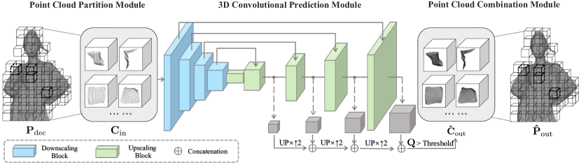
Fig. 2: The architecture of the proposed model. We first split the point cloud into cubes. Then the neural network is used to predict the occupancy probability for each voxel. Finally, we obtain the refined point clouds based on the predicted probabilities.

3.1 Point Cloud Partition Module

Point clouds collected from reality can have millions of points. It is extremely difficult to refine all these points at one time. Therefore, partition methods are required to split point clouds for subsequent operations. In this paper, we follow the partition method described in [13] and [14]. The decoded point clouds stored with disordered coordinates are first converted to a 3D volumetric representation $\mathbf{P}_{\mathrm{dec}}$ using voxelization. The voxelized point clouds are defined on regular 3D grids, whereas a voxel can be deemed as the 3D counterpart to the pixel in 2D. Given that our model tackles the geometry information of the point clouds, we binarize $\mathbf{P}_{\mathrm{dec}}$ to obtain the geometry inputs, where occupied voxels are set to $1$, and the remaining voxels are set to $0$.

After obtaining $\mathbf{P}_{\mathrm{dec}}$, we divide it into small non-overlapped cubes $\mathbf{C}_{\mathrm{in}}\in\{0,1\}^{l\times w\times h}$. Symbols $l$, $w$, and $h$ are the spatial sizes of cubes, respectively. By converting the decoded point clouds into cubes, 3D geometry information of point clouds can be easily extracted by neural networks.

3.2 3D Convolutional Prediction Module

Multi-Scale Probability Prediction. After obtaining the split cubes $\mathbf{C}_{\mathrm{in}}$, our model refines these cubes by predicting the lost points caused by quantization and correcting the positions of existing points. Point clouds compressed with different bit rates contain large varying degrees of distortion. Therefore, to tackle point clouds with arbitrary distortion, the up-sampling ratio of the refinement network should not be explicitly limited. To achieve this, we use a 3D convolutional neural network to generate the occupancy probability cubes $\mathbf{Q}\in\mathbb{R}^{l\times w\times h}$ from input cubes $\mathbf{C}_{\mathrm{in}}$. By learning to predict the geometry distributions of the ground-truth cubes, our network can handle decompressed point clouds with varying degrees of distortion.

The architecture of the proposed network is shown in Fig. 2. This network takes $\mathbf{C}_{\mathrm{in}}$ as inputs and generates the probability cubes $\mathbf{Q}$. Each value in $\mathbf{Q}$ indicates the occupancy probability of the corresponding voxel. The predicting process is described as follows:

$$\mathbf{Q}=\mathcal{G}(\mathbf{C}_{\mathrm{in}}),$$ (1)

where $\mathcal{G}$ denotes the 3D convolutional geometry network. We design $\mathcal{G}$ using a U-Net structure. The encoder consists of four downscaling blocks. Each block downsamples the inputs with a factor of $2$. In the decoder, we use transposed convolutional layers with a stride of two to upscale the feature maps. Skip connections are applied to concatenate the feature maps of the encoder and that of the decoder. The concatenated feature maps are sent to the next upscaling block. A sigmoid function is used as the activation function of the final layer, which enables obtaining values between $0$ and $1$.

We generate the final occupancy probability $\mathbf{Q}$ in a coarse-to-fine manner. Each decoder layer produces a probability cube with the corresponding scale. The obtained probability cube is then up-sampled using the nearest neighbor interpolation method. We generate the final prediction by summing the contribution of each scale. We show that the performance can be further improved by using such coarse-to-fine architecture in Sec. 4.3.

Loss Function. To train the model $\mathcal{G}$, we apply the same partition operation to the ground-truth point clouds and obtain binarized cubes $\mathbf{C}_{\mathrm{gt}}$. We calculate the cross-entropy loss $\mathcal{L}$ to minimize the difference between the refined occupancy probability $\mathbf{Q}$ and the ground-truth probability $\mathbf{C}_{\mathrm{gt}}$ as below:

$$\mathcal{L}=-\frac{1}{N}\sum_{n=0}^{N}\big{[}c_{n}\text{log}(q_{n})+(1-c_{n})\text{log}(1-q_{n})\big{]},$$ (2)

where $c_{n}$ and $q_{n}$ are the $n$-th voxel in $\mathbf{C}_{\mathrm{gt}}$ and $\mathbf{Q}$, respectively. Symbol $N=l\times w\times h$ denotes the number of voxels in a cube.

Determination Strategies. After obtaining $\mathbf{Q}$, the geometry-refined cubes $\mathbf{\hat{C}}_{\mathrm{out}}$ can be calculated using a suitable threshold $\sigma$. The choice of the threshold $\sigma$ is important since it directly determines the final prediction results. In this paper, we test two strategies including: 1) a fixed threshold $\sigma$ and 2) an adaptive $\sigma$ determined by the number of occupied voxels in $\mathbf{C}_{\mathrm{gt}}$. For the first strategy, we select the threshold with the highest performance on the training point clouds as our fixed threshold. Here we use a fixed threshold $\sigma=0.98$ for all experiments. Voxels with probabilities larger than $\sigma$ will be set as occupied. Experiments show that by using the fixed threshold, our model is able to achieve state-of-the-art results. For the second strategy, we use an adaptive $\sigma$, which selects top-k voxels to ensure the refined cubes $\mathbf{\hat{C}}_{\mathrm{out}}$ to have the same number of points as that of $\mathbf{C}_{\mathrm{gt}}$. This setting requires additional bit streams to transmit the number of points in each ground-truth cube. The experiments in Sec. 4.2 prove the transmission cost is negligible. Meanwhile, this strategy can obtain additional RD performance gain compared with the fixed threshold. It can still obtain even more RD performance gains with negligible increased bits. See Sec. 4.2 for more details.

3.3 Point Cloud Combination Module

After obtaining $\mathbf{\hat{C}}_{\mathrm{out}}$, we combine these cubes to generate the geometry-refined point clouds $\mathbf{\hat{P}}_{\mathrm{out}}$. The combination operation first converts the relative coordinate $\mathbf{x}^{r}_{n}=(x^{r}_{n},y^{r}_{n},z^{r}_{n})$ of each voxel in each cube to the absolute coordinate $\mathbf{x}_{n}=(x_{n},y_{n},z_{n})$. Let us assume a cube with global index $\mathbf{i}=(i,j,k)$, the absolute coordinate is calculated as follows:

$$\mathbf{x}_{n}=\mathbf{i}\odot\mathbf{l}+\mathbf{x}^{r}_{n},$$ (3)

where $\odot$ is the element-wise multiplication. Symbol $\mathbf{l}=(l,w,h)$ is the spatial size of cubes. After obtaining the absolute coordinate $\mathbf{x}_{n}$, we copy the binary values in cubes $\mathbf{\hat{C}}_{\mathrm{out}}$ to the corresponding voxels in $\mathbf{\hat{P}}_{\mathrm{out}}$ to obtain the final refined point clouds.

4 Experiments

4.1 Implementation Details

Datasets. We use three datasets for training and evaluation.

• 8iVFB [15]. The 8i Voxelized Full Bodies is a dynamic point cloud dataset. There are four sequences in the dataset. Each sequence contains around 300 frames recording the movements of a human subject. The resolution is provided at 10-bit with a cube of $1024\times 1024\times 1024$ voxels.

• MVUB [16]. The Microsoft Voxelized Upper Bodies is a dynamic voxelized point cloud dataset. Five subjects are contained in this dataset. The upper bodies of these subjects are captured. Each sequence contains around 250 frames. The resolutions are provided at 9-bit and 10-bit. We use 9-bit point clouds in the experiments.

• ODHM [19]. The Owlii Dynamic Human Mesh dataset contains four sequences. For each sequence, it contains around $400$ frames. The resolution is provided at 11-bit.

Training Details. The longdress and loot sequences in the 8iVFB dataset are used for training. We randomly select $60$ frames from the two sequences to construct the training set. The latest version of MPEG-TMC13 (V14.0) [4] is used to obtain the decompressed point clouds at different bit rates. We train our model with decoded point clouds of multiple bit rates to improve its generalization. The 3D block size $l\times w\times h$ is set to $64\times 64\times 64$. By default, we use a Adam optimizer with a learning rate $0.001$. The batch size is set to $64$.

Evaluation Details. We evaluate the performance of our proposed model following the MPEG common test conditions [8]. Except for the two training point cloud sequences, the other sequences of the above three datasets are used for testing. The evaluation frame of each sequence is provided in Table 1. We use point-to-point error (D1) [8] to evaluate the geometry distortion. It calculates the distance between points in a point cloud and the corresponding nearest points in another point cloud. Both Peak Signal-to-Noise Ratio (PSNR) and Bjontegaard-Delta Peak Signal-to-Noise Rate (BDPSNR) [7] are used to report the D1 distortion values. Higher scores indicate lower distortions.

Fig. 3: Rate-distortion curves of different methods in several point clouds. For each curve, the horizontal axis represents the bit rate, while the vertical axis represents the PSNR score.

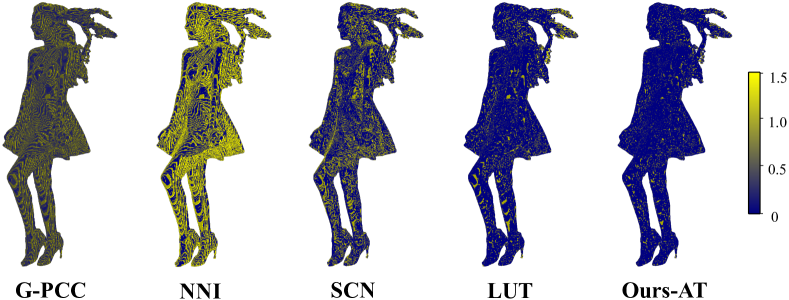
Fig. 4: Visualization of point-to-point errors. The heat maps indicate the degrees of distortion. Blue represents the lowest distortion, while yellow represents the highest distortion.

Table 1: Quantitative evaluation of different post-processing models. The BDPSNR gains against G-PCC (octree) are provided. We compare our model with several state-of-the-art methods including NNI, SCN [6], and LUT [5]. Two determination strategies are evaluated: the fixed threshold $\sigma=0.98$ (Ours-FT) and the adaptive threshold (Ours-AT).

Dataset	Point Cloud	#Frame	Depth	Size	NNI	SCN	LUT	Ours-FT	Ours-AT
MVUB	andrew	0032	9	281k	2.92	4.18	6.47	7.64	8.47
	david	0032	9	305k	2.77	3.92	6.75	7.95	7.19
	phil	0032	9	333k	2.79	4.34	6.39	7.88	8.55
	ricardo	0032	9	207k	2.93	4.56	6.83	7.98	9.10
	sarah	0032	9	301k	2.82	4.10	6.65	7.84	8.68
8iVFB	redandblack	1550	10	757k	1.27	2.86	5.38	9.14	9.56
	soldier	0690	10	1,089k	1.24	2.69	5.99	9.64	9.36
ODHM	basketball_player	0200	11	2,925k	0.41	2.38	5.66	10.41	10.85
	dancer	0001	11	2,592k	0.59	2.65	5.77	9.99	10.47
	exercise	0001	11	2,391k	0.59	2.76	5.65	10.01	10.47
	model	0001	11	2,458k	0.77	3.03	5.37	9.04	9.63
	Average				1.74	3.41	6.08	8.87	9.30

4.2 Performance Comparison

In this subsection, we compare our model with several state-of-the-art methods: the Nearest-Neighbor Interpolation (NNI), Sparse Convolutional Network (SCN) [6], and LookUp Table (LUT) [5]. NNI is a commonly used point cloud up-sampling method. It sets all children of each parent node as occupied. Different from NNI, LUT up-samples point clouds with lookup tables calculated from self-similarities. SCN is a learning-based method, which predicts the occupancy probabilities for the children of each voxel. We retrain SCN using the same training datasets as ours for fair comparisons. In SCN, we follow their original setting to train a new model for each bit rate. Different from it, the advantage of ours is that we use a single model to deal with all bit rates.

Table 2: Quantitative evaluation of post-processing models. The BDPSNR gains against G-PCC (octree) are provided.

Dataset	MVUB	8iVFB	ODHM	Average
Baseline-FT	6.51	9.45	9.42	8.10
Ours-FT	7.86	9.39	9.86	8.87

Quantitative Comparison. The quantitative comparison results are shown in Table 1. We provide the BDPSNR scores for each of post-processing models against G-PCC. We also display the performance of our model with two determination strategies. It can be seen that our method outperforms other methods at all test sets. Although our model is trained on 10-bit point clouds, it still achieves good results on diverse datasets with different sizes. The Rate-Distortion (R-D) curves are shown in Fig. 3. These curves provide the performance of the models at different bit rates. It can be seen that our model can significantly improve the quality of the decompressed point clouds, especially at low bit rates. Although LUT can obtain considerable performance gains at high bit rates, the performance decreases dramatically at low bit rates.

Qualitative Comparisons. To intuitively show the distortions of the generated point clouds, we provide the error maps in Fig. 4. In these error maps, yellow and blue are used to indicate the highest and the lowest distortions, respectively. It can be seen that our method can effectively reduce the errors between the decoded and the original point clouds.

Discussion on Determination Strategies. We use two different determination strategies in this paper: the fixed threshold (Ours-FT) and the adaptive threshold (Ours-AT). The fixed threshold does not bring any bitstream overhead, while the adaptive one needs to transmit the number of points in each ground-truth cubes. We compressed the point numbers with a lossless codec: Lempel-Ziv-Markov chain-Algorithm (LZMA) [20]. According to the statistics, the adaptive strategy only needs to transmit a code stream less than 0.01bpp. Both RD curves in Fig.3 and BDPSNR gains in Table 1 show that the adaptive strategy can always bring additional performance gain with negligible bits increase.

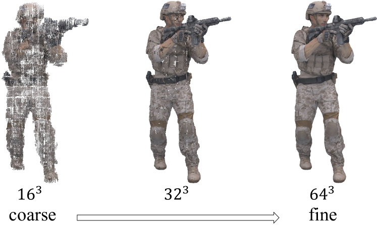
Fig. 5: Visualization of the multi-scale probabilities predicted by our model. Form left to right, we show the point clouds combined by cubes with resolutions $16^{3}$, $32^{3}$, and $64^{3}$.

4.3 Ablation Study

We verify the effectiveness of the multi-scale probability prediction operation. A baseline model is trained with a U-Net architecture by removing the coarse-to-fine structure from our model. We train the baseline model using the same setting as ours. The evaluation results are shown in Table 2. It can be observed that our multi-scale probability prediction operation always brings additional performance gains. We also show the intermediate results obtained from the multi-scale probability cubes in Fig. 5. A clear coarse-to-fine generation process can be observed, which verify our hypothesis.

5 Conclusion

We propose a deep post-processing network which can effectively enhance the quality of decompressed point clouds. A 3D convolutional network is applied for predicting the occupancy probabilities of each position, in order to recover lost points caused by quantization. Moreover, we use a coarse-to-fine architecture to progressively generate the final predictions. Different from previous methods, our model is successfully trained once to deal with point clouds with large varying degrees of distortion. Experimental results show that our model can generate geometry-refined point clouds, which significantly improves the visual quality. Code is available at https://github.com/fxqzb/Deep-Geometry-Post-Processing.

Acknowledgment. This work was supported in part by National Natural Science Foundation of China (No. 62172021), and in part by Shenzhen Fundamental Research Program (GXWD20201231165807007-20200806163656003).

References

- [1] Ruwen Schnabel and Reinhard Klein, “Octree-based point-cloud compression,” in Proceedings of the 3rd Eurographics/IEEE VGTC Conference on Point-Based Graphics, 2006, pp. 111–121.
- [2] Yan Huang, Jingliang Peng, C-C Jay Kuo, and M Gopi, “A generic scheme for progressive point cloud coding,” IEEE Transactions on Visualization and Computer Graphics, vol. 14, no. 2, pp. 440–453, 2008.
- [3] Julius Kammerl, Nico Blodow, Radu Bogdan Rusu, Suat Gedikli, Michael Beetz, and Eckehard Steinbach, “Real-time compression of point cloud streams,” in 2012 IEEE International Conference on Robotics and Automation, 2012, pp. 778–785.
- [4] MPEG 3D Graphics Coding, “G-PCC test model v14,” Standard, ISO/IEC JTC1/SC29/WG7 output document N00094, 2021.
- [5] T. M. Borges, D. C. Garcia, and R. L. de Queiroz, “Fractional super-resolution of voxelized point clouds,” TechRxiv. Preprint., 2021.
- [6] Anique Akhtar, Wen Gao, Xiang Zhang, Li Li, Zhu Li, and Shan Liu, “Point cloud geometry prediction across spatial scale using deep learning,” in 2020 IEEE International Conference on Visual Communications and Image Processing (VCIP), 2020, pp. 70–73.
- [7] Gisle Bjontegaard, “Calculation of average PSNR differences between RD-curves,” Standard, VCEG input document M33, 2001.
- [8] MPEG 3D Graphics Coding, “Common test conditions for G-PCC,” Standard, ISO/IEC JTC1/SC29/WG7 output document N00106, 2021.
- [9] Sebastian Schwarz, Marius Preda, Vittorio Baroncini, Madhukar Budagavi, Pablo Cesar, Philip A Chou, Robert A Cohen, Maja Krivokuća, Sébastien Lasserre, Zhu Li, et al., “Emerging mpeg standards for point cloud compression,” IEEE Journal on Emerging and Selected Topics in Circuits and Systems, vol. 9, no. 1, pp. 133–148, 2019.
- [10] Tianxin Huang and Yong Liu, “3D point cloud geometry compression on deep learning,” in Proceedings of the 27th ACM International Conference on Multimedia, 2019, pp. 890–898.
- [11] Zhirong Wu, Shuran Song, Aditya Khosla, Fisher Yu, Linguang Zhang, Xiaoou Tang, and Jianxiong Xiao, “3D ShapeNets: A deep representation for volumetric shapes,” in Proceedings of the IEEE Conference on Computer Vision and Pattern Recognition, 2015, pp. 1912–1920.
- [12] Angel X Chang, Thomas Funkhouser, Leonidas Guibas, Pat Hanrahan, Qixing Huang, Zimo Li, Silvio Savarese, Manolis Savva, Shuran Song, Hao Su, et al., “ShapeNet: An information-rich 3D model repository,” arXiv preprint arXiv:1512.03012, 2015.
- [13] Maurice Quach, Giuseppe Valenzise, and Frederic Dufaux, “Improved deep point cloud geometry compression,” in 2020 IEEE 22nd International Workshop on Multimedia Signal Processing (MMSP), 2020, pp. 1–6.
- [14] Jianqiang Wang, Hao Zhu, Haojie Liu, and Zhan Ma, “Lossy point cloud geometry compression via end-to-end learning,” IEEE Transactions on Circuits and Systems for Video Technology, vol. 31, no. 12, pp. 4909–4923, 2021.
- [15] Eugene d’Eon, Bob Harrison, Taos Myers, and Philip A Chou, “8i voxelized full bodies - A voxelized point cloud dataset,” Standard, ISO/IEC JTC1/SC29 Joint WG11/WG1 (MPEG/JPEG) input document WG11M40059/WG1M74006, 2017.
- [16] Charles Loop, Qin Cai, S Orts Escolano, and Philip A Chou, “Microsoft voxelized upper bodies - A voxelized point cloud dataset,” Standard, ISO/IEC JTC1/SC29 Joint WG11/WG1 (MPEG/JPEG) input document M38673/M72012, 2016.
- [17] Wei Jia, Li Li, Anique Akhtar, Zhu Li, and Shan Liu, “Convolutional neural network-based occupancy map accuracy improvement for video-based point cloud compression,” IEEE Transactions on Multimedia, 2021.
- [18] Wei Jia, Li Li, Zhu Li, and Shan Liu, “Deep learning geometry compression artifacts removal for video-based point cloud compression,” International Journal of Computer Vision, vol. 129, no. 11, pp. 2947–2964, 2021.
- [19] Xu Yi, Lu Yao, and Wen Ziyu, “Owlii dynamic human mesh sequence dataset,” Standard, ISO/IEC JTC1/SC29/WG11 input document M41658, 2017.
- [20] Jyrki Alakuijala, Evgenii Kliuchnikov, Zoltan Szabadka, and Lode Vandevenne, “Comparison of Brotli, Deflate, Zopfli, LZMA, LZHAM and Bzip2 compression algorithms,” Technical report, Google Inc, 2015.