Symmetry-protected exceptional and nodal points in non-Hermitian systems

Abstract

One of the unique features of non-Hermitian (NH) systems is the appearance of non-Hermitian degeneracies known as exceptional points (EPs). The extensively studied defective EPs occur when the Hamiltonian becomes non-diagonalizable. Aside from this degeneracy, we show that NH systems may host two further types of degeneracies, namely, non-defective EPs and ordinary (Hermitian) nodal points. The non-defective EPs manifest themselves by i) the diagonalizability of the NH Hamiltonian at these points, ii) the non-diagonalizability of the Hamiltonian along certain intersections of these points and iii) instabilities in the Jordan decomposition when approaching the points from certain directions. We demonstrate that certain discrete symmetries, namely parity-time, parity-particle-hole, and pseudo-Hermitian symmetry, guarantee the occurrence of both defective and non-defective EPs. We extend this list of symmetries by including the NH time-reversal symmetry in two-band systems. Two-band and four-band models exemplify our findings. Through an example, we further reveal that ordinary nodal points may coexist with defective EPs in NH models when the above symmetries are relaxed.

Introduction.

Despite violating the axioms of quantum mechanics, non-Hermitian (NH) Hamiltonians offer compelling descriptions for numerous interacting/open systems in various fields of physics Bender (2005); Ashida et al. (2020); Alexandre et al. (2020); Sayyad et al. (2021, 2022). The underlying physics of these effective Hamiltonians goes beyond the realm of Hermitian physics and has been immensely studied lately Bergholtz et al. (2021); Zhou et al. (2018); Berry (2004); Heiss (2012); Xu et al. (2017a); Kozii and Fu ; Carlström and Bergholtz (2018); Cerjan et al. (2019); Carlström et al. (2019); Stålhammar et al. (2019); Zhang et al. (2021); Yang et al. (2020); Ghorashi et al. (2021a, b). Aside from unraveling rich physics, the properties of NH systems are well-reflected in abstract mathematical frameworks, including homotopy theory Wojcik et al. (2020); Hu and Zhao (2021); Li and Mong (2021); Wojcik et al. ; Hu et al. and K-theory Gong et al. (2018); Zhou and Lee (2019); Kawabata et al. (2019a). These frameworks provide a reliable toolbox to understand the exotic properties of NH systems and distinguish their behavior from Hermitian physics.

Noticeable distinctions of NH Hamiltonians from their Hermitian counterparts include the appearance of exceptional points (EPs), as NH degeneracies. While one generally should satisfy $n-1$ complex constraints to realize EPs of order $n$ (EP$n$s), at which the Hamiltonian casts a Jordan block, recent studies have shown that the presence of certain discrete symmetries, such as parity-time ($\mathcal{PT}$), parity-particle-hole ($\cal CP$), or pseudo-Hermiticity ($\rm psH$) symmetry, reduces the total number of constraints Budich et al. (2019); Yoshida et al. (2019); Okugawa and Yokoyama (2019); Zhou et al. (2019); Szameit et al. (2011); Kimura et al. (2019); Delplace et al. (2021); Mandal and Bergholtz (2021); Stålhammar and Bergholtz (2021); Crippa et al. (2021); Sayyad and Kunst (2022). Although the main focus of these studies was on characterizing symmetry-induced restrictions on defective EPs, drawing a link between discrete symmetries and non-defective degeneracies associated with the NH Hamiltonian beyond case studies have received little attention. Furthermore, while there is a near consensus on calling defective degeneracies Xu et al. (2017b); Kawabata et al. (2019b) defective EPs , non-defective degeneracies in NH systems are referred to as diabolic points Keck et al. (2003); Xue et al. (2020); Wiersig (2022); Cui et al. , Fermi points Yang et al. (2021), Dirac points and vortex points Shen et al. (2018). These non-defective degeneracies are different in nature, as both Dirac points and vertex points might appear in the vicinity of defective EPs, while diabolic points and Fermi points are similar to (Hermitian) ordinary nodal points (ONPs).

Recalling their mathematical origin, EPs were introduced by Kato as isolated singularities of systems depending on one complex variable Kato (1995), and they were recently classified into type I EPs and type II EPs Ashida et al. (2020). EPs of type I are degeneracies with or without algebraic singularities reminiscent of defective EPs and ONPs, while type II EPs are defined as points in the complex plane where the Jordan normal form is unstable, i.e., the eigenprojectors have a pole. While the appearance and existence of degeneracies reminiscent of type I EPs have been studied extensively, type II EPs have hitherto been overlooked in the literature.

In this letter, we introduce a natural extension of type II EPs to higher dimensions, dubbed non-defective EPs. We present that the correct criterion for detecting non-defective EPs is the form of the Hamiltonian matrix in the vicinity of these degenerate points: Non-defective EPs are surrounded by defective EPs along certain intersections such that the Hamiltonian matrix casts a Jordan block in certain directions away from the non-defective EPs. Furthermore, we show that the Jordan decomposition is singular at these points when approaching the points from certain directions, emphasizing that non-defective EPs indeed are reminiscent of the type II EPs in Ref. Ashida et al., 2020. To characterize the role of symmetries in witnessing NH degeneracies, we study the coexistence of defective and non-defective EP$n$s in two-, three- and four-band models in the presence of psH, ${\cal PT}$ or ${\cal CP}$ symmetry. Additionally, we show that symmetry-protected non-defective EP2s may also appear in models with non-Hermitian time-reversal symmetry. Finally, we find that defective EPs may coexist with ONPs instead of non-defective EPs when lifting symmetry constraints. We illustrate this finding with a fine-tuned example.

Finding possibilities to detect ONPs and (non-)defective EPs may pave the way to advance applications of Hermitian and non-Hermitian topological properties in various fields of research. For instance, topological lasers are one of the platforms which owe their success to either Hermitian Wittek et al. (2017); Zeng et al. (2020) or non-Hermitian St-Jean et al. (2017); Parto et al. (2018); Harari et al. (2018); Bandres et al. (2018) topological properties. Moreover, our systems, especially $\cal PT$-symmetric models, are experimentally feasible as they can be implemented in experimental optical setups with balanced gain and loss effectively Özdemir et al. (2019). Exploring the role of EPs in $\cal PT$-symmetric optical systems has already unraveled many interesting phenomena, such as unidirectional invisibility Regensburger et al. (2012), induced mode-transition by encircling EPs Doppler et al. (2016), loss induced optical transparency Guo et al. (2009), and stable single-mode lasing in multi-mode optical setups Feng et al. (2014); Hodaei et al. (2015).

Symmetry-stabilized (non-)defective EPs.

A generic $n$-band Hamiltonian can be decomposed as $\operatorname{\mathcal{H}}=d_{\mu}\Upsilon^{\mu}$, where $\mu\in\{0,\cdots,n^{2}-1\}$, $d_{\mu}$ are continuously differentiable complex-valued functions of the lattice momentum $\mathbf{k}$, $\Upsilon^{0}$ denotes the identity matrix of order $n$ and $\boldsymbol{\Upsilon}$ is the basis of the $SU(n)$ group, which consists of three Pauli matrices when $n=2$, eight Gell-Mann matrices when $n=3$, and fifteen generalized Gell-Mann matrices when $n=4$ (see supplemental materials (SM) for the explicit presentation of these matrices SuppMat ). The Hamiltonian $\operatorname{\mathcal{H}}$ displays $\cal PT$ symmetry with generator ${\cal PT}$, $\cal CP$ symmetry with generator ${\cal CP}$, or $\rm psH$ with generator $\varsigma$, if it satisfies one of the following relations, namely,

$${\cal PT}: \quad\operatorname{\mathcal{H}}(\mathbf{k})=({\cal PT})\operatorname{\mathcal{H}}^{*}(\mathbf{k})({\cal PT})^{-1},$$ (1)

$${\cal CP}: \quad\operatorname{\mathcal{H}}(\mathbf{k})=-({\cal CP})\operatorname{\mathcal{H}}^{*}(\mathbf{k})({\cal CP})^{-1},$$ (2)

$${\rm psH}: \quad\operatorname{\mathcal{H}}(\mathbf{k})=\varsigma\operatorname{\mathcal{H}}^{\dagger}(\mathbf{k})\varsigma^{-1}.$$ (3)

These symmetry considerations reduce the number of nonzero $d_{\mu}$ values. More precisely, for each basis matrix $\Upsilon^{\mu}$ merely a real or imaginary part of $d_{\mu}$ remains nonzero, i.e., only one real-valued function $d_{\mu}$ per each dimension of $\Upsilon^{\mu}$ survives Sayyad and Kunst (2022). Trivial band touching points occur when the traceless part of $\operatorname{\mathcal{H}}$ becomes a Null matrix ($[0]_{n\times n}$), i.e., all of the nonzero $d_{\mu}$ values for $\mu>0$ must vanish, which means that one needs to satisfy $n^{2}-1$ real constraints. For $n=2,3,4$, we have collected these $d_{\mu}$’s for each symmetry operation along side a choice for its generator in Tables 1, 2, and 3, respectively.

The $n-1$ complex constraints to find defective EP$n$s can be expressed in terms of the traces and the determinant of $\operatorname{\mathcal{H}}$, which for two-, three-, and four-band models, respectively, read Sayyad and Kunst (2022)

$$n=2: \quad\eta^{2b}=\mathop{\mathrm{tr}}[\operatorname{\mathcal{H}}]^{2}-4\det[\operatorname{\mathcal{H}}],$$ (4)

$$n=3: \begin{cases}\eta^{3b}&=\frac{1}{2}\left(\mathop{\mathrm{tr}}[{\cal H}]^{2}-3\mathop{\mathrm{tr}}[{\cal H}^{2}]\right),\\ \nu^{3b}&=\frac{1}{2}\left(54\det[{\cal H}]-5\mathop{\mathrm{tr}}[{\cal H}]^{3}+9\mathop{\mathrm{tr}}[{\cal H}]\mathop{\mathrm{tr}}[{\cal H}^{2}]\right),\end{cases}$$ (5)

$$n=4: \begin{cases}\eta^{4b}&=-3ac+b^{2}+12d,\\ \nu^{4b}&=27a^{2}d-9abc+2b^{3}-72bd+27c^{2},\\ \kappa^{4b}&=a^{3}-4ab+8c,\end{cases}$$ (6)

where $a=\mathop{\mathrm{tr}}[{\cal H}]$, $b=\big{(}(\mathop{\mathrm{tr}}[{\cal H}])^{2}-\mathop{\mathrm{tr}}[{\cal H}^{2}]\big{)}/2$, $d=\det[{\cal H}]$ and $c=\left(\mathop{\mathrm{tr}}[{\cal H}]^{3}-3\mathop{\mathrm{tr}}[{\cal H}]\mathop{\mathrm{tr}}[{\cal H}^{2}]+2\mathop{\mathrm{tr}}[{\cal H}^{3}]\right)/6$. We refer to the SM for details on how to derive these expressions SuppMat .

In the presence of ${\cal PT}$, ${\cal CP}$ and psH symmetry, some of these constraints are automatically satisfied leaving us with exactly $n-1$ real constraints, cf. Tables 1, 2 and 3 Sayyad and Kunst (2022). It is notable that at trivial solutions (${\bf d}=0$), all traces and the determinant of $\operatorname{\mathcal{H}}$ acquire zero values and subsequently, the constraints in Eqs. (4)-(6) are also satisfied. As a result, the trivial solutions mark non-defective EP$n$s with the binding signature that $\operatorname{\mathcal{H}}$ is diagonalizable at these points. Perturbing the system away from these non-defective points along intersections at which the constraints vanish brings the Hamiltonian into a non-diagonalizable structure. We set this behavior as a criterion to detect non-defective EPs. We note that this is opposed to the situation in which trivial solutions are isolated, and thus band touching points behave similarly to Hermitian degeneracies, i.e., ONPs.

The diagonalizability of the Hamiltonian at non-defective EPs enables us to map our NH Hamiltonians into their Hermitian counterparts with nodal points. In addition, having $n^{2}-1$ nonzero $d_{\mu}$’s as in Hermitian systems enforces non-defective EPs to always appear in pairs. This statement originates from the Poincaré-Hopf theorem Mathai and Thiang (2017), as the number of nonzero $d_{\mu}$ functions equals the dimension of the vector space ($n^{2}-1$), cf. last columns in Tables 1, 2, and 3 Poincare .

Table 1: Summarized symmetries, their generators and their associated constraints to find defective and non-defective EP2s in two-band systems.

Symm.		Generator		Constr. def. EP2s		Constr. non-def. EP2s
${\cal PT}$		${\mathbbm{1}}$		$\eta^{2b}_{R}=0$		$d_{xR}=d_{yI}=d_{zR}=0$
${\cal CP}$		${\mathbbm{1}}$		$\eta^{2b}_{R}=0$		$d_{xI}=d_{yR}=d_{zI}=0$
psH		${\rm adiag}[1,1]$		$\eta^{2b}_{R}=0$		$d_{xR}=d_{yI}=d_{zI}=0$
TRS†		${\rm adiag}[1,-1]$		$\eta^{2b}_{R}=\eta^{2b}_{I}=0$		$d_{xa}=d_{ya}=d_{za}=0$

Here we use either $d_{j}=d_{jR}+\mathrm{i}d_{jI}$ or $d_{j}=d_{js}+d_{ja}$, where $d_{js}(d_{ja})$ is (anti-)symmetric with respect to $\mathbf{k}\to-\mathbf{k}$. $\eta^{2b}$ is given in Eq. (4) with $\eta^{2b}=\eta^{2b}_{R}+\mathrm{i}\eta^{2b}_{I}$.

Aside from $\cal PT$, $\cal CP$ and $\rm psH$ symmetries, a particular non-Hermitian time-reversal symmetry, known as TRS^†, in two-band systems may also give rise to realizing non-defective EPs. To evidently see this behavior, we recall that respecting TRS^† symmetry imposes $\operatorname{\mathcal{H}}(-\mathbf{k})={\cal C}_{+}\operatorname{\mathcal{H}}^{\dagger}(\mathbf{k}){\cal C}^{\dagger}_{+}$. This non-(momentum)-local transformation does not reduce the number of non-vanishing (real/imaginary) parts of $d_{\mu}$. However, when ${\cal C}_{+}=\mathrm{i}\sigma_{y}$, it enforces all symmetric parts of $d_{\mu}$ to become zero. We further know that right at time-reversal invariant momenta (TRIM), e.g., $\mathbf{k}_{\rm TRIM}=\{(0,0),(0,\pi),(\pi,0),(\pi,\pi)\}$ on the square Brillouin zone, anti-symmetric functions vanish. Therefore, at $\mathbf{k}_{\rm TRIM}$ both real and imaginary parts of anti-symmetric $d_{\mu}$ functions become zero, which gives rise to observing non-defective EPs in the spectra of two-band TRS^†-symmetric $\operatorname{\mathcal{H}}$, cf. Table 1.

Table 2: Summarized symmetries, their generators and their associated constraints to find defective and non-defective EP3s in three-band systems.

Symm.		Generator		Constr. def. EP3s		Constr. non-def. EP3s
${\cal PT}$		${\rm diag}[1,-1,1]$		$\eta^{3b}_{R}=0\,\&\,\nu^{3b}_{R}=0$		$d_{1R}=d_{4I}=d_{2I}=d_{5R}=d_{3R}=d_{6I}=d_{7R}=d_{8R}=0$
${\cal CP}$		${\rm diag}[1,-1,1]$		$\eta^{3b}_{R}=0\,\&\,\nu^{3b}_{I}=0$		$d_{1I}=d_{4R}=d_{2R}=d_{5I}=d_{3I}=d_{6R}=d_{7I}=d_{8I}=0$
psH		${\rm diag}[1,-1,1]$		$\eta^{3b}_{R}=0\,\&\,\nu^{3b}_{R}=0$		$d_{1I}=d_{4I}=d_{2R}=d_{5R}=d_{3I}=d_{6I}=d_{7R}=d_{8R}=0$

Here we use $d_{j}=d_{jR}+\mathrm{i}d_{jI}$. Complex valued $\eta^{3b}$ and $\nu^{3b}$ constraints are given in Eq. (5) with $\alpha^{3b}=\alpha^{3b}_{R}+\mathrm{i}\alpha^{3b}_{I}$ for $\alpha\in\{\eta,\nu\}$.

Table 3: Summarized symmetries, their generators and their associated constraints to get defective and non-defective EP4s in four-band systems.

Symm.		Generator		Constr. def. EP4s		Constr. non-def. EP4s
${\cal PT}$		${\rm diag}[1,-1,1,-1]$		$\eta^{4b}_{R}=0\,\&\,\nu^{4b}_{R}=0\,\&\,\kappa^{4b}_{R}=0$		$d_{1R}=d_{2I}=d_{3R}=d_{4R}=d_{5I}=d_{6R}=d_{7I}=d_{8R}=0$ $d_{9I}=d_{10I}=d_{11R}=d_{12I}=d_{13R}=d_{14R}=d_{15R}=0$
${\cal CP}$		${\rm diag}[1,-1,1,-1]$		$\eta^{4b}_{R}=0\,\&\,\nu^{4b}_{R}=0\,\&\,\kappa^{4b}_{I}=0$		$d_{1I}=d_{2R}=d_{3I}=d_{4I}=d_{5R}=d_{6I}=d_{7R}=d_{8I}=0$ $d_{9R}=d_{10R}=d_{11I}=d_{12R}=d_{13I}=d_{14I}=d_{15I}=0$
psH		${\rm diag}[1,-1,1,-1]$		$\eta^{4b}_{R}=0\,\&\,\nu^{4b}_{R}=0\,\&\,\kappa^{4b}_{R}=0$		$d_{1I}=d_{2R}=d_{3I}=d_{4I}=d_{5R}=d_{6I}=d_{7I}=d_{8R}=0$ $d_{9I}=d_{10I}=d_{11R}=d_{12I}=d_{13R}=d_{14R}=d_{15R}=0$

Here we use $d_{j}=d_{jR}+\mathrm{i}d_{jI}$. Complex valued $\eta^{4b}$, $\nu^{4b}$ and $\kappa^{4b}$ constraints are given in Eq. (6) with $\alpha^{4b}=\alpha^{4b}_{R}+\mathrm{i}\alpha^{4b}_{I}$ for $\alpha\in\{\eta,\nu,\kappa\}$.

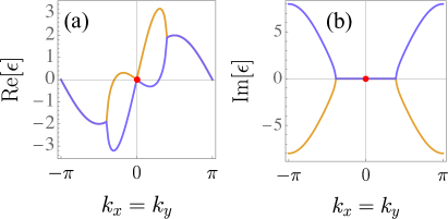
Figure 1: Real part (a) and imaginary part (b) of spectra for Eq. (7) along $k_{x}=k_{y}$ with $k_{z}=\pi/2$. Red points indicate non-defective EPs. Here we set $t=V=\lambda_{0}=1.0$.

Before moving on to examples, we note that the different number of constraints that need to be satisfied to find symmetry-protected defective and non-defective EP$n$s also result in a different codimension of these EPs. Here, the codimension is given by the difference between the total dimension of the system and the dimension of the exceptional feature. Equivalently, the codimension corresponds precisely to the number of nonvanishing constraints. In particular, while the presence of ${\cal PT}$, ${\cal CP}$ and psH symmetries reduces the number of real constraints for finding defective EP$n$s to $n-1$, the number of real constraints to detect non-defective EP$n$s is $n^{2}-1$. As a consequence, in the case of $n=2$, defective EP2s have codimension one, whereas non-defective EP2s have codimension three. Therefore, the latter appear as points in three-dimensional systems, whereas defective EP2s appear as two-dimensional surfaces. For the TRS^† invariant two-band model, the codimension is two, and hence the defective EP2s are curves connected at the TRIMs.

Examples for the coexistence of defective and non-defective EPs.

We start with introducing a two-band ${\cal PT}$-symmetric Weyl-like tight-binding model described by

$$\operatorname{\mathcal{H}}_{\cal PT}^{2b} =d_{0}\Upsilon^{0}+d_{xR}\Upsilon^{1}+\mathrm{i}d_{yI}\Upsilon^{2}+d_{zR}\Upsilon^{3}$$

$$=2\lambda_{0}\sin{\left(k_{x}\right)}\Upsilon^{0}+2t\sin{\left(k_{x}\right)}\Upsilon^{1}+2t\sin{\left(k_{y}\right)}\Upsilon^{3}$$

$$+\mathrm{i}\left\{2t\cos{\left(k_{z}\right)}+2V\left[2-\cos{\left(k_{x}\right)}-\cos{\left(k_{y}\right)}\right]\right\}\Upsilon^{2}.$$ (7)

Here $\lambda_{0}$, $t$ and $V$ are real-valued parameters. The real and imaginary parts of the band structure are shown in Figs. 1(a) and (b), respectively.

Non-defective EPs appear when all components of the Hamiltonian, except $d_{0}$, vanish. More specifically, these degeneracies emerge when the solutions of $d_{xR}=0$ (at $k_{x}=n\pi$ with $n\in\mathbb{Z}$), $d_{yI}=0$ (orange curves in Fig. 2), and $d_{zR}=0$ (grey line) intersect. Red points at $\mathbf{k}=\left(0,0,\pm\pi/2\right)$ in Fig. 2 exemplify such solutions. Note that the criterion for detecting non-defective EPs is satisfied for the red points in Fig. 2 as they are surrounded by defective EPs (dashed blue curves), residing on $\eta^{2b}_{R}=0$, where $\eta^{2b}_{R}$ is the real part of $\eta^{2b}$ in Eq. (4).

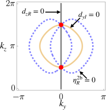
Figure 2: Solutions of $d_{yI}$ (orange), $d_{zR}$ (gray), and $\eta_{R}^{2b}$ (dashed blue) at $k_{x}=0$, which is a solution to $d_{xR}=0$. Red points at $\mathbf{k}=(0,0,\pm\pi/2)$ indicate the intersection between solutions to $\eta_{R}^{2b}=d_{yI}=d_{zR}=0$, and are non-defective EPs. Here we set $t=V=\lambda_{0}=1.0$.

Along the defective EPs, defined by $d_{xR}^{2}+d_{zR}^{2}=d_{yI}^{2}$, the Jordan decomposition reads $\operatorname{\mathcal{H}}_{\mathcal{PT}}^{2b}=SJS^{-1}$ with $S=(s_{1},s_{2})$, where

$$s_{1} =\begin{pmatrix}\frac{\sqrt{t^{4}\left[2-\cos{\left(2k_{x}\right)}-\cos{\left(2k_{y}\right)}\right]}-\sqrt{2}t^{2}\sin{\left(k_{x}\right)}}{\sqrt{2}t^{2}\sin{\left(k_{y}\right)}}\\ 1\end{pmatrix},$$ (8)

$$s_{2} =\begin{pmatrix}\frac{\sqrt{2}\sqrt{t^{4}\left[2-\cos{\left(2k_{x}\right)}-\cos{\left(2k_{y}\right)}\right]}-2t^{2}\sin{\left(k_{x}\right)}}{4t^{3}\sin{\left(k_{y}\right)}^{2}}\\ 0\end{pmatrix},$$ (9)

$$J =\begin{pmatrix}2\lambda_{0}\sin{\left(k_{x}\right)}&1\\ 0&2\lambda_{0}\sin{\left(k_{x}\right)}\end{pmatrix}.$$ (10)

The second column in the transformation matrix, $s_{2}$, has a singularity when $k_{x}$ and $k_{y}$ goes to $n\pi$ simultaneously, corresponding exactly to the non-defective EP. Hence, the Jordan decomposition is unstable at the non-defective EPs.

We further note that the defective EPs separate two regions in the real part of spectrum, where $\text{Re}[\Delta\epsilon]=0$ and $\text{Re}[\Delta\epsilon]\neq 0$ with $\Delta\epsilon$ the difference between the two energy bands as shown in Fig. 1(a). Regions where $\text{Re}[\Delta\epsilon]=0$ are sometimes referred to as NH bulk real-Fermi states, which merely appear in NH systems Bergholtz et al. (2021). In the SM, we show that besides these bulk Fermi states, this model also hosts states on the boundary SuppMat . Therefore, there is a coexistence between defective and non-defective EPs as well as between bulk Fermi states and boundary states.

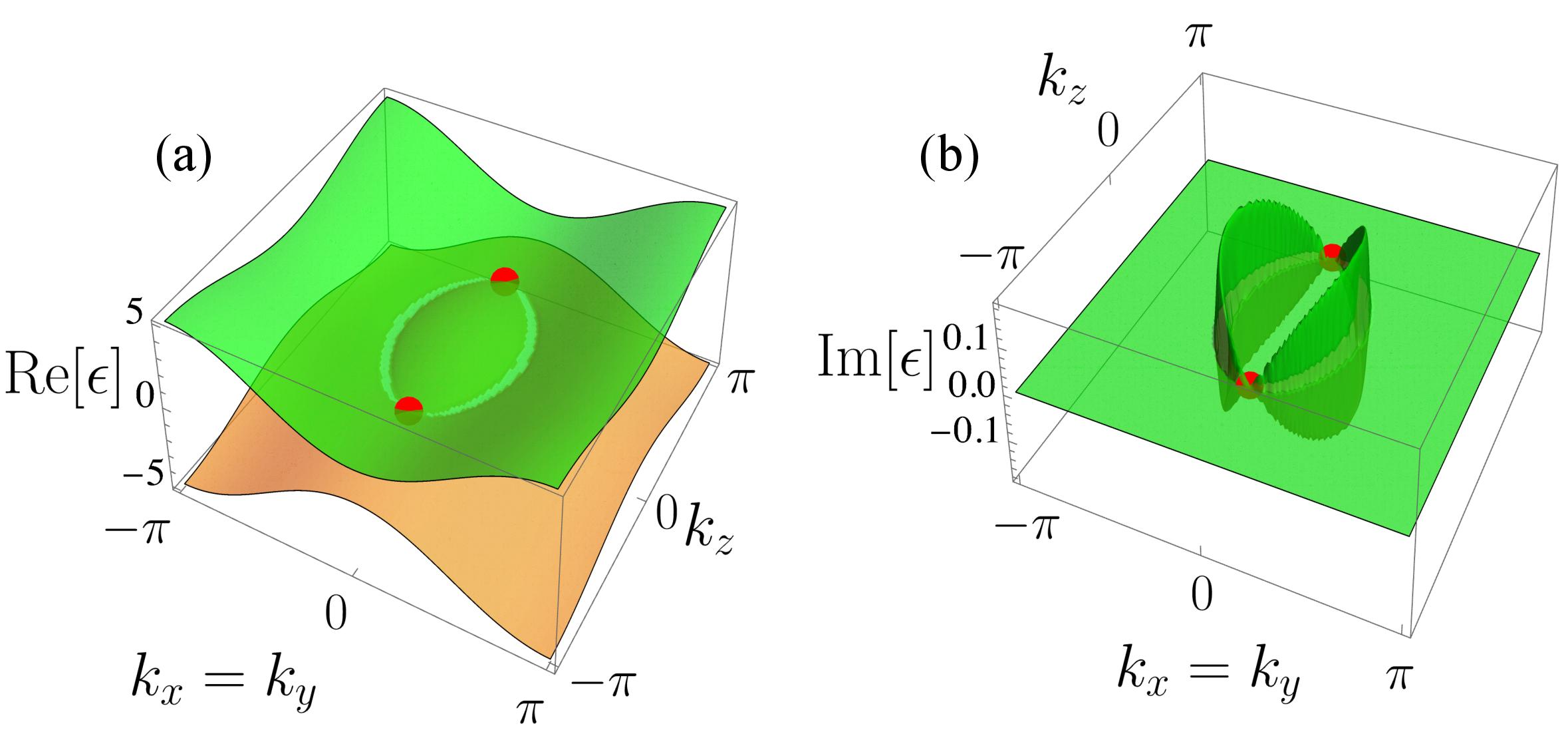
Figure 3: Real (a) and imaginary (b) parts of band structure for $\operatorname{\mathcal{H}}_{\rm psH}^{4b}$ in Eq. (11) along $k_{x}=k_{y}$ and $k_{z}$. Note that both bands are doubly degenerate. Red points indicate non-defective EPs at $\mathbf{k}=(0,0,\pm k_{0})$. Here we set $t=t_{z}=1.0$, $\lambda_{Ixx}=\lambda_{Ixy}=0.15$, $m^{\prime}_{I}=-0.27$ and $k_{0}=\pi/2$.

Let us now turn to a four-band model. We consider a Dirac-like $\rm psH$-symmetric model described by

$$\operatorname{\mathcal{H}}_{\rm psH}^{4b}= t\left[\cos{\left(k_{x}\right)}+\cos{\left(k_{y}\right)}-2\right]\left(\frac{2}{\sqrt{3}}\Upsilon^{14}+\sqrt{\frac{2}{3}}\Upsilon^{15}\right)$$

$$+t_{z}\left[\cos{\left(k_{z}\right)}-\cos{\left(k_{0}\right)}\right]\left[\frac{2}{\sqrt{3}}\Upsilon^{14}+\sqrt{\frac{2}{3}}\Upsilon^{15}\right]$$

$$+\mathrm{i}\lambda_{Ixy}\sin{\left(k_{y}\right)}(\Upsilon^{3}+\Upsilon^{4})$$

$$+\mathrm{i}\lambda_{Ixx}\sin{\left(k_{x}\right)}(\Upsilon^{9}+\Upsilon^{10})$$

$$+\mathrm{i}m^{\prime}_{I}\sin{\left(k_{z}\right)}\left[\cos{\left(k_{x}\right)}-\cos{\left(k_{y}\right)}\right]\left(\Upsilon^{7}-\Upsilon^{12}\right),$$ (11)

where $t$, $t_{z}$, $\lambda_{Ixy}$, $\lambda_{Ixx}$, and $m_{I}^{{}^{\prime}}$ are real-valued parameters. This model is a $\rm psH$ generalization of the tight-binding model studied in Ref. Kargarian et al., 2016. The trivial band touching points for obtaining the null form of the traceless part of $\operatorname{\mathcal{H}}_{\rm psH}^{4b}$ in Eq. (11) are located at $\mathbf{k}=\mathbf{k}_{\rm psH}=(0,0,\pm k_{0})$. Right at these points and on lines connecting these points, constraints for realizing EP4s, summarized in Table 3 and given in Eq. (6), are also satisfied. Hence, points at $\mathbf{k}=\mathbf{k}_{\rm psH}$ in our $\rm psH$-symmetric model are non-defective EP4s. We present these nodal points (red spheres) in the band structure of $\operatorname{\mathcal{H}}_{\rm psH}^{4b}$ in Fig. 3. The real part of the spectra (a) shows that two arc-shaped surfaces with (non)zero real (imaginary) parts are terminated by the non-defective EPs as well as the defective exceptional lines. These surfaces are the aforementioned NH bulk real-Fermi surfaces. While our model hosts bulk Fermi surfaces, boundary states are not stable, similar to its Hermitian counterpart Kargarian et al. (2016).

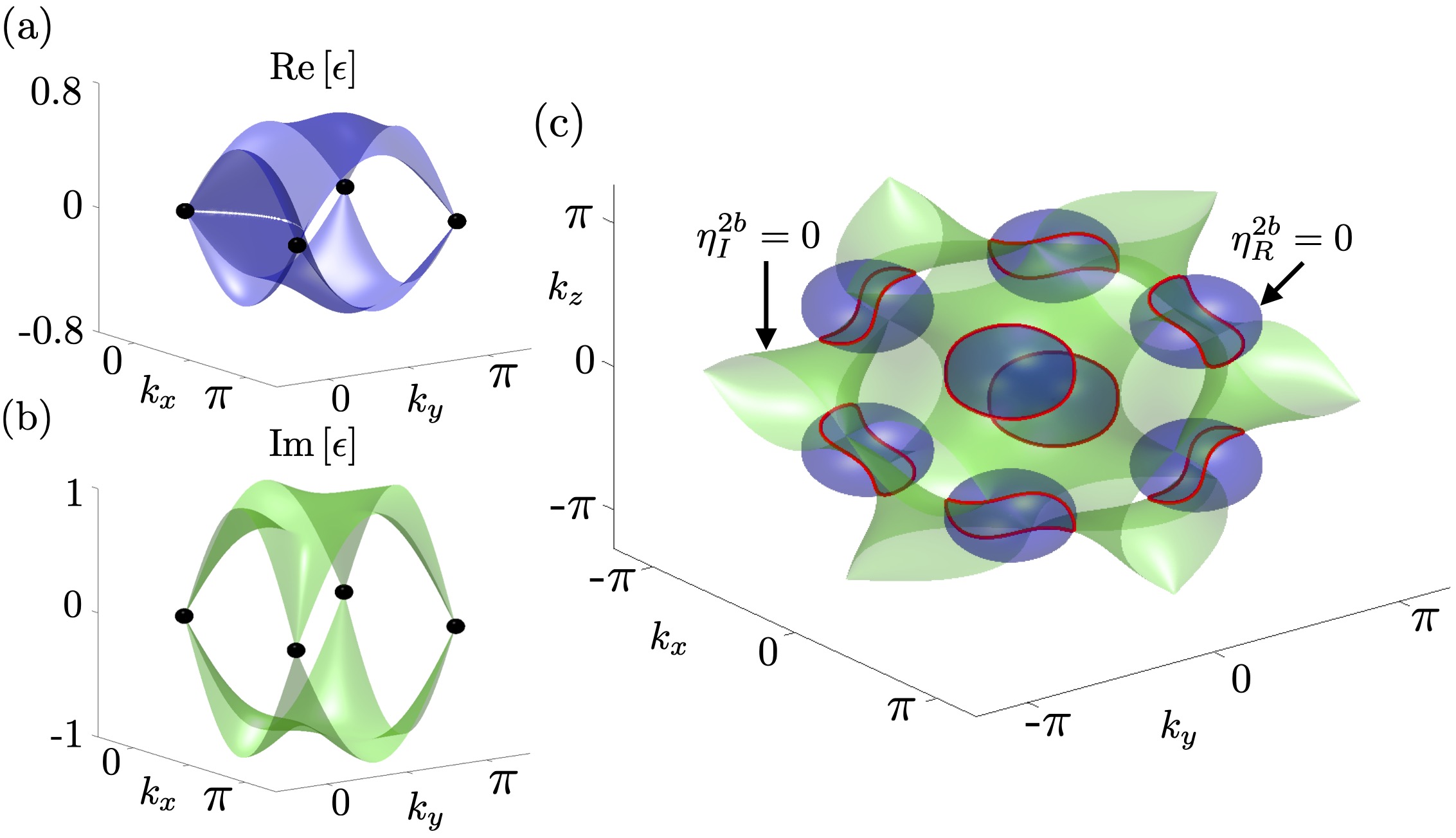
Figure 4: Real (a) and imaginary (b) parts of band structure for $\operatorname{\mathcal{H}}_{\rm ONP}^{\rm 2b}$ in Eq. (12) along $k_{z}=\pi$. (c) Solutions of the real (blue spheres) and imaginary (green manifold) parts of $\eta^{2b}$ in Eq. (4). Red closed lines in (c) present the intersection of these manifolds and correspond to defective EPs. Black points in panels (a), (b) indicate ONPs. For visibility purposes, merely a corner of Brillouin zone is shown in panels (a), (b).

Searching for the coexistence of ONPs and defective EPs.

So far, we have explored how the presence of one of the ${\cal PT}$, ${\cal CP}$ or $\rm psH$ symmetries leads to the general coexistence of defective and non-defective EPs. In the remaining, we address whether ONPs may also exist in NH spectra. For this purpose, we lift (discrete) symmetry restrictions such that some (or all) $d_{\mu}$’s have real and imaginary parts. We emphasize that in this situation, in contrast to the EPs in the previous sections, band degeneracies are generally unstable to small perturbations . This is because finding solutions to ${\bf d}=0$ generally requires satisfying $n^{2}-1$ complex constraints. Consequently, the appearance of ONPs in NH models is vulnerable to the fine-tuning of parameters. Nevertheless, we show in the following that this setting provides a platform to observe ONPs.

To illustrate our idea, we introduce a two-band model given by

$$\operatorname{\mathcal{H}}_{\rm ONP}^{2b} =\sin(k_{x})\left[1/2+\mathrm{i}\cos(k_{y})\right]\Upsilon^{1}$$

$$+\sin(k_{y})\left[1/2+\mathrm{i}\cos(k_{z})\right]\Upsilon^{2}$$

$$+\sin(k_{z})\left[1/2+\mathrm{i}\cos(k_{x})\right]\Upsilon^{3}.$$ (12)

Fig. 4 exhibits real (a) and imaginary (b) parts of the energy dispersion of this system along $k_{z}=\pi$. The black points in these panels mark real and imaginary band touching points, located at $k_{x,y,z}^{\rm ONP}=\pm n\pi$. Even though at these momenta the traceless part of $\operatorname{\mathcal{H}}_{\rm ONP}^{2b}$ becomes a null matrix, we emphasize that ${\bf k}={\bf k}^{\rm ONP}$ indicates the location of ONPs and not non-defective EPs. The reason for this statement lies in the fact that the criterion for the emergence of non-defective EPs is not satisfied, i.e., no defective EPs reside close to ${\bf k}^{\rm ONP}$. This can be seen from Fig. 4 (c) in which we present defective EPs, red curves, as the intersection between $\text{Re}[\eta^{2b}]=0$, blue spheres, and $\text{Im}[\eta^{2b}]=0$, green manifold. Fig. 4 (c) reveals that defective EPs do not cross ${\bf k}={\bf k}^{\rm ONP}$ and thus the black points at ${\bf k}^{\rm ONP}$ indeed correspond to ONPs. Consequently, $H^{2b}_{\text{ONP}}$ is diagonalizable at ${\bf k}={\bf k}^{\rm ONP}$ and in any small neighborhood surrounding the point.

Aside from these ONPs in the momentum-space, introducing models that host boundary states connecting ONPs in NH systems is theoretically feasible. We present an example of such a model in the SM SuppMat .

Conclusion.

Despite the intense focus on NH systems in recent studies, the possibility of realizing different types of EPs has hitherto been overlooked. The present work shows that two different types of EPs, dubbed defective and non-defective EPs, may coexist in various setups of physical importance. Concretely, we show that non-defective EPs are stabilized by certain symmetries, including $\cal PT$, $\cal CP$, $\rm psH$, and time-reversal symmetry. To resolve the confusion in the current literature, where non-defective EPs are mixed up with ONPs, we have in this work introduced a clear criterion to distinguish these concepts. We also highlight this difference in example models.

Even though the models we discuss in this work are experimentally tractable, we do not expect a difference in the experimental signatures of non-defective EPs and ONPs when single-particle, non-interacting Hamiltonians are explored. Investigating interacting/coupled systems may allow identifying distinct footprints of non-defective EPs and ONPs in experiments.

Acknowledgements.

M.S. is supported by the Swedish Research Council (VR) and the Wallenberg Academy Fellows program of the Knut and Alice Wallenberg Foundation. L.R. acknowledges the support from the Knut and Alice Wallenberg foundation under grant no. 2017.0157.

Appendix A Bases matrices for two-, three-, and four-band systems

A.1 Basis matrices for two-band systems

The basis matrices for two-band systems are Pauli matrices which read

$$\Upsilon^{1}=\begin{pmatrix}0&1\\ 1&0\end{pmatrix},\,\,\Upsilon^{2}=\begin{pmatrix}0&-\mathrm{i}\\ \mathrm{i}&0\end{pmatrix},\,\,\Upsilon^{3}=\begin{pmatrix}1&0\\ 0&-1\end{pmatrix}.$$ (13)

A.2 Basis matrices for three-band systems

The basis matrices for three-band systems are the Gell-Mann matrices, that span the Lie algebra of the SU(3) group,

$$\Upsilon^{1} =\begin{pmatrix}0&-\mathrm{i}&0\\ \mathrm{i}&0&0\\ 0&0&0\end{pmatrix},\quad\Upsilon^{2}=\begin{pmatrix}0&0&-\mathrm{i}\\ 0&0&0\\ \mathrm{i}&0&0\end{pmatrix},$$ (14)

$$\Upsilon^{3} =\begin{pmatrix}0&0&0\\ 0&0&-\mathrm{i}\\ 0&\mathrm{i}&0\end{pmatrix},\quad\Upsilon^{4}=\begin{pmatrix}0&1&0\\ 1&0&0\\ 0&0&0\end{pmatrix},$$ (15)

$$\Upsilon^{5} =\begin{pmatrix}0&0&1\\ 0&0&0\\ 1&0&0\end{pmatrix},\quad\Upsilon^{6}=\begin{pmatrix}0&0&0\\ 0&0&1\\ 0&1&0\end{pmatrix},$$ (16)

$$\Upsilon^{7} =\begin{pmatrix}1&0&0\\ 0&-1&0\\ 0&0&0\end{pmatrix},\quad\Upsilon^{8}=\begin{pmatrix}\frac{1}{\sqrt{3}}&0&0\\ 0&\frac{1}{\sqrt{3}}&0\\ 0&0&-\frac{2}{\sqrt{3}}\end{pmatrix}.$$ (17)

A.3 Basis matrices for four-band systems

The basis matrices for four-band systems are the generalized Gell-Mann matrices, that span the Lie algebra of the SU(4) group,

$$\Upsilon^{1} =\begin{pmatrix}0&-\mathrm{i}&0&0\\ \mathrm{i}&0&0&0\\ 0&0&0&0\\ 0&0&0&0\\ \end{pmatrix},\quad\Upsilon^{2}=\begin{pmatrix}0&0&-\mathrm{i}&0\\ 0&0&0&0\\ \mathrm{i}&0&0&0\\ 0&0&0&0\\ \end{pmatrix},$$ (18)

$$\Upsilon^{3} =\begin{pmatrix}0&0&0&-\mathrm{i}\\ 0&0&0&0\\ 0&0&0&0\\ \mathrm{i}&0&0&0\\ \end{pmatrix},\quad\Upsilon^{4}=\begin{pmatrix}0&0&0&0\\ 0&0&-\mathrm{i}&0\\ 0&\mathrm{i}&0&0\\ 0&0&0&0\\ \end{pmatrix},$$ (19)

$$\Upsilon^{5} =\begin{pmatrix}0&0&0&0\\ 0&0&0&-\mathrm{i}\\ 0&0&0&0\\ 0&\mathrm{i}&0&0\\ \end{pmatrix},\quad\Upsilon^{6}=\begin{pmatrix}0&0&0&0\\ 0&0&0&0\\ 0&0&0&-\mathrm{i}\\ 0&0&\mathrm{i}&0\\ \end{pmatrix},$$ (20)

$$\Upsilon^{7} =\begin{pmatrix}0&1&0&0\\ 1&0&0&0\\ 0&0&0&0\\ 0&0&0&0\\ \end{pmatrix},\quad\Upsilon^{8}=\begin{pmatrix}0&0&1&0\\ 0&0&0&0\\ 1&0&0&0\\ 0&0&0&0\\ \end{pmatrix},$$ (21)

$$\Upsilon^{9} =\begin{pmatrix}0&0&0&1\\ 0&0&0&0\\ 0&0&0&0\\ 1&0&0&0\\ \end{pmatrix},\quad\Upsilon^{10}=\begin{pmatrix}0&0&0&0\\ 0&0&1&0\\ 0&1&0&0\\ 0&0&0&0\\ \end{pmatrix},$$ (22)

$$\Upsilon^{11} =\begin{pmatrix}0&0&0&0\\ 0&0&0&1\\ 0&0&0&0\\ 0&1&0&0\\ \end{pmatrix},\quad\Upsilon^{12}=\begin{pmatrix}0&0&0&0\\ 0&0&0&0\\ 0&0&0&1\\ 0&0&1&0\\ \end{pmatrix},$$ (23)

$$\Upsilon^{13} =\begin{pmatrix}1&0&0&0\\ 0&-1&0&0\\ 0&0&0&0\\ 0&0&0&0\\ \end{pmatrix},\,\Upsilon^{14}=\begin{pmatrix}\frac{1}{\sqrt{3}}&0&0&0\\ 0&\frac{1}{\sqrt{3}}&0&0\\ 0&0&-\frac{2}{\sqrt{3}}&0\\ 0&0&0&0\\ \end{pmatrix},$$ (24)

$$\Upsilon^{15} =\begin{pmatrix}\frac{1}{\sqrt{6}}&0&0&0\\ 0&\frac{1}{\sqrt{6}}&0&0\\ 0&0&\frac{1}{\sqrt{6}}&0\\ 0&0&0&-\sqrt{\frac{3}{2}}\\ \end{pmatrix}.$$ (25)

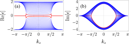
Figure S1: Real parts (a) and imaginary parts (b) of spectra for Eq. (7) with open boundary condition in the $y$ direction and $k_{x}=0$. Red lines present boundary states. Here we set $t=V=\lambda_{0}=1.0$.

Appendix B Derivation of constraints to find EP$n$s

Here we briefly summarize how to derive Eqs. (4)-(6) in the main text, where these constraints were originally derived in Ref. Sayyad and Kunst, 2022. There it was shown that the characteristic polynomial of an $n$-band NH matrix can be expressed in terms of its determinant and traces. Indeed, for two-, three- and four-band matrices, these polynomials read

$$F^{2b}(\lambda) =\lambda^{2}-\mathop{\mathrm{tr}}[\mathcal{H}]\lambda+\det[\mathcal{H}]=0,$$ (26)

$$F^{3b}(\lambda) =\lambda^{3}-\mathop{\mathrm{tr}}[\mathcal{H}]\lambda^{2}+\frac{\mathop{\mathrm{tr}}[\mathcal{H}]^{2}-\mathop{\mathrm{tr}}[\mathcal{H}^{2}]}{2}\lambda-\det[\mathcal{H}]=0,$$ (27)

$$F^{4b}(\lambda) =\lambda^{4}-a\lambda^{3}+b\lambda^{2}-c\lambda+d=0,$$ (28)

where

$$a =\mathop{\mathrm{tr}}[\mathcal{H}],\quad b=\frac{\mathop{\mathrm{tr}}[\mathcal{H}]^{2}-\mathop{\mathrm{tr}}[\mathcal{H}^{2}]}{2},\quad d=\det[\mathcal{H}],$$ (29)

$$c =\frac{\mathop{\mathrm{tr}}[\mathcal{H}]^{3}-3\mathop{\mathrm{tr}}[\mathcal{H}]\mathop{\mathrm{tr}}[\mathcal{H}^{2}]+2\mathop{\mathrm{tr}}[\mathcal{H}^{3}]}{6},$$ (30)

and $\lambda$ are the eigenvalues.

To find degeneracies, the discriminant $D[\mathcal{H}]$ of these characteristic polynomials need to be set to zero. The discriminants read

$$D[\mathcal{H}^{2b}] =\mathop{\mathrm{tr}}[\mathcal{H}]^{2}-4\det[\mathcal{H}],$$ (31)

$$D[\mathcal{H}^{3b}] =-\frac{1}{27}[4(\eta^{3b})^{3}+(\nu^{3b})^{2}],$$ (32)

$$D[\mathcal{H}^{4b}] =\frac{1}{27}[4(\eta^{4b})^{3}-(\nu^{4b})^{2}],$$ (33)

where $\eta^{3b}$ and $\nu^{3b}$, and $\eta^{4b}$ and $\nu^{4b}$ are given in Eqs. (5) and (6) in the main text, respectively. From here, we immediately see that setting the discriminants in Eqs. (31) and (32) to zero gives us the constraints in Eqs. (4) and (5) in the main text, respectively. In the case of the four-band model, we note that for all roots of the discriminant to coincide, not only $\eta^{4b}=0$ and $\nu^{4b}=0$ need to be satisfied, but also $\kappa^{4b}=0$, where $\kappa^{4b}$ is defined in Eq. (6) in the main text. We refer to Ref. Sayyad and Kunst, 2022 for a more detailed discussion on this point.

Appendix C Spectra of the two-band model with open boundary condition

In addition to the properties of momentum-dependent spectra for ${\cal H}_{\cal PT}^{\rm 2b}$ in Fig. 1, we present real (a) and imaginary (b) parts of the energy dispersion with open boundary condition in the $y$ direction plotted in Fig. S1. The figure exhibits boundary states, red lines, well-separated from the bulk states (blue lines) when $|k_{z}|>\pi/2$.

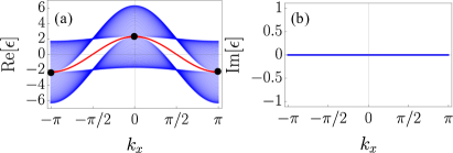
Figure S2: Real parts (a) and imaginary parts (b) of spectra for Eq. (34) with open boundary condition in the $y$ direction and at $k_{z}=0$. Red lines present boundary states. Black points mark ONPs. Here we set $t=V=1.0,\lambda_{0}=2.3$.

Appendix D Realizing Hermitian boundary states in non-Hermitian systems

Here we present a non-Hermitian tight-binding model hosting Hermitian boundary states, which connects ONPs with zero imaginary parts.

Our model Hamiltonian reads

$$\operatorname{\mathcal{H}}_{\rm edg}^{\rm 2b}= \lambda_{0}\cos(k_{x})\Upsilon^{0}-\mathrm{i}V\left[1-\cos(k_{z})\right]\Upsilon^{1}$$

$$+\left[2V\cos(k_{y})-2t\cos(k_{x})\right]\Upsilon^{1}$$

$$-2t\sin(k_{y})\Upsilon^{2}-2t\sin(k_{z})\Upsilon^{3},$$ (34)

where $\lambda_{0}$, $t$ and $V$ are real-valued coupling constants. Along $k_{z}=0$, the above Hamiltonian is fully Hermitian. As a result, nodal points, which live on the $(k_{x},k_{y})$ plane, are band touching points with zero imaginary parts. For instance, these ordinary nodal points appear at $\mathbf{k}_{\rm ONPs}=(\pm n\pi,\pm n\pi,0)$ with $n\in\operatorname{\mathbb{Z}}$ when $t=V$. Considering the open boundary condition along the $y$ axis and at $k_{z}=0$ results in mid-gap boundary states, red lines in Fig. S2(a), which connects $\mathbf{k}_{\rm ONPs}$.

References

- Bender (2005) Carl. M. Bender, “Non-hermitian quantum field theory,” International Journal of Modern Physics A 20, 4646 (2005).
- Ashida et al. (2020) Yuto Ashida, Zongping Gong, and Masahito Ueda, “Non-hermitian physics,” Advances in Physics 69, 249 (2020).
- Alexandre et al. (2020) Jean Alexandre, John Ellis, and Peter Millington, “-symmetric non-hermitian quantum field theories with supersymmetry,” Phys. Rev. D 101, 085015 (2020).
- Sayyad et al. (2021) Sharareh Sayyad, Jinlong Yu, Adolfo G. Grushin, and Lukas M. Sieberer, “Entanglement spectrum crossings reveal non-hermitian dynamical topology,” Phys. Rev. Research 3, 033022 (2021).
- Sayyad et al. (2022) Sharareh Sayyad, Julia D. Hannukainen, and Adolfo G. Grushin, “Non-hermitian chiral anomalies,” Phys. Rev. Research 4, L042004 (2022).
- Bergholtz et al. (2021) Emil J. Bergholtz, Jan Carl Budich, and Flore K. Kunst, “Exceptional topology of non-hermitian systems,” Rev. Mod. Phys. 93, 015005 (2021).
- Zhou et al. (2018) Hengyun Zhou, Chao Peng, Yoseob Yoon, Chia Wei Hsu, Keith A. Nelson, Liang Fu, John D. Joannopoulos, Marin Soljačić, and Bo Zhen, “Observation of bulk fermi arc and polarization half charge from paired exceptional points,” Science 359, 1009 (2018).
- Berry (2004) M. V. Berry, “Physics of nonhermitian degeneracies,” Czechoslovak Journal of Physics 54, 1039 (2004).
- Heiss (2012) W D Heiss, “The physics of exceptional points,” J. Phys. A: Math. Theor. 45, 444016 (2012).
- Xu et al. (2017a) Yong Xu, Sheng-Tao Wang, and L.-M. Duan, “Weyl exceptional rings in a three-dimensional dissipative cold atomic gas,” Phys. Rev. Lett. 118, 045701 (2017a).
- (11) Vladyslav Kozii and Liang Fu, “Non-hermitian topological theory of finite-lifetime quasiparticles: Prediction of bulk fermi arc due to exceptional point,” arXiv:1708.05841 .
- Carlström and Bergholtz (2018) Johan Carlström and Emil J. Bergholtz, “Exceptional links and twisted fermi ribbons in non-hermitian systems,” Phys. Rev. A 98, 042114 (2018).
- Cerjan et al. (2019) Alexander Cerjan, Sheng Huang, Mohan Wang, Kevin P. Chen, Yidong Chong, and Mikael C. Rechtsman, “Experimental realization of a Weyl exceptional ring,” Nature Photonics 13, 623 (2019), 1808.09541 .
- Carlström et al. (2019) Johan Carlström, Marcus Stålhammar, Jan Carl Budich, and Emil J. Bergholtz, “Knotted non-hermitian metals,” Phys. Rev. B 99, 161115 (2019).
- Stålhammar et al. (2019) Marcus Stålhammar, Lukas Rødland, Gregory Arone, Jan Carl Budich, and Emil J. Bergholtz, “Hyperbolic Nodal Band Structures and Knot Invariants,” SciPost Phys. 7, 19 (2019).
- Zhang et al. (2021) Xiao Zhang, Guangjie Li, Yuhan Liu, Tommy Tai, Ronny Thomale, and Ching Hua Lee, “Tidal surface states as fingerprints of non-Hermitian nodal knot metals,” Communications Physics 4, 1 (2021).
- Yang et al. (2020) Zhesen Yang, Ching-Kai Chiu, Chen Fang, and Jiangping Hu, “Jones polynomial and knot transitions in hermitian and non-hermitian topological semimetals,” Phys. Rev. Lett. 124, 186402 (2020).
- Ghorashi et al. (2021a) Sayed Ali Akbar Ghorashi, Tianhe Li, Masatoshi Sato, and Taylor L. Hughes, “Non-hermitian higher-order dirac semimetals,” Phys. Rev. B 104, L161116 (2021a).
- Ghorashi et al. (2021b) Sayed Ali Akbar Ghorashi, Tianhe Li, and Masatoshi Sato, “Non-hermitian higher-order weyl semimetals,” Phys. Rev. B 104, L161117 (2021b).
- Wojcik et al. (2020) Charles C. Wojcik, Xiao-Qi Sun, Tomá š Bzdušek, and Shanhui Fan, “Homotopy characterization of non-hermitian hamiltonians,” Phys. Rev. B 101, 205417 (2020).
- Hu and Zhao (2021) Haiping Hu and Erhai Zhao, “Knots and non-hermitian bloch bands,” Phys. Rev. Lett. 126, 010401 (2021).
- Li and Mong (2021) Zhi Li and Roger S. K. Mong, “Homotopical characterization of non-hermitian band structures,” Phys. Rev. B 103, 155129 (2021).
- (23) Charles C. Wojcik, Kai Wang, Avik Dutt, Janet Zhong, and Shanhui Fan, “Eigenvalue topology of non-hermitian band structures in two and three dimensions,” arXiv:2111.09977 .
- (24) Haiping Hu, Shikang Sun, and Shu Chen, “Knot topology of exceptional point and non-hermitian no-go theorem,” arXiv:2111.11346 .
- Gong et al. (2018) Zongping Gong, Yuto Ashida, Kohei Kawabata, Kazuaki Takasan, Sho Higashikawa, and Masahito Ueda, “Topological phases of non-hermitian systems,” Phys. Rev. X 8, 031079 (2018).
- Zhou and Lee (2019) Hengyun Zhou and Jong Yeon Lee, “Periodic table for topological bands with non-hermitian symmetries,” Phys. Rev. B 99, 235112 (2019).
- Kawabata et al. (2019a) Kohei Kawabata, Ken Shiozaki, Masahito Ueda, and Masatoshi Sato, “Symmetry and topology in non-hermitian physics,” Phys. Rev. X 9, 041015 (2019a).
- Budich et al. (2019) Jan Carl Budich, Johan Carlström, Flore K. Kunst, and Emil J. Bergholtz, “Symmetry-protected nodal phases in non-hermitian systems,” Phys. Rev. B 99, 041406 (2019).
- Yoshida et al. (2019) Tsuneya Yoshida, Robert Peters, Norio Kawakami, and Yasuhiro Hatsugai, “Symmetry-protected exceptional rings in two-dimensional correlated systems with chiral symmetry,” Phys. Rev. B 99, 121101 (2019).
- Okugawa and Yokoyama (2019) Ryo Okugawa and Takehito Yokoyama, “Topological exceptional surfaces in non-hermitian systems with parity-time and parity-particle-hole symmetries,” Phys. Rev. B 99, 041202 (2019).
- Zhou et al. (2019) Hengyun Zhou, Jong Yeon Lee, Shang Liu, and Bo Zhen, “Exceptional surfaces in pt-symmetric non-hermitian photonic systems,” Optica 6, 190 (2019).
- Szameit et al. (2011) Alexander Szameit, Mikael C. Rechtsman, Omri Bahat-Treidel, and Mordechai Segev, “-symmetry in honeycomb photonic lattices,” Phys. Rev. A 84, 021806 (2011).
- Kimura et al. (2019) Kazuhiro Kimura, Tsuneya Yoshida, and Norio Kawakami, “Chiral-symmetry protected exceptional torus in correlated nodal-line semimetals,” Phys. Rev. B 100, 115124 (2019).
- Delplace et al. (2021) Pierre Delplace, Tsuneya Yoshida, and Yasuhiro Hatsugai, “Symmetry-protected multifold exceptional points and their topological characterization,” Phys. Rev. Lett. 127, 186602 (2021).
- Mandal and Bergholtz (2021) Ipsita Mandal and Emil J. Bergholtz, “Symmetry and higher-order exceptional points,” Phys. Rev. Lett. 127, 186601 (2021).
- Stålhammar and Bergholtz (2021) Marcus Stålhammar and Emil J. Bergholtz, “Classification of exceptional nodal topologies protected by symmetry,” Phys. Rev. B 104, L201104 (2021).
- Crippa et al. (2021) L. Crippa, J. C. Budich, and G. Sangiovanni, “Fourth-order exceptional points in correlated quantum many-body systems,” Phys. Rev. B 104, L121109 (2021).
- Sayyad and Kunst (2022) Sharareh Sayyad and Flore K. Kunst, “Realizing exceptional points of any order in the presence of symmetry,” Phys. Rev. Research 4, 023130 (2022).
- Xu et al. (2017b) Yong Xu, Sheng-Tao Wang, and L.-M. Duan, “Weyl exceptional rings in a three-dimensional dissipative cold atomic gas,” Phys. Rev. Lett. 118, 045701 (2017b).
- Kawabata et al. (2019b) Kohei Kawabata, Takumi Bessho, and Masatoshi Sato, “Classification of exceptional points and non-hermitian topological semimetals,” Phys. Rev. Lett. 123, 066405 (2019b).
- Note (1) Except in Ref. Shen et al. (2018) where ‘hybrid points’ have also been introduced based on the asymptotic dispersion relations close to defective degeneracies. Note that branch cuts do not terminate at these points Yang et al. (2021).
- Keck et al. (2003) F Keck, HJ Korsch, and S Mossmann, “Unfolding a diabolic point: a generalized crossing scenario,” Journal of Physics A: Mathematical and General 36, 2125 (2003).
- Xue et al. (2020) Haoran Xue, Qiang Wang, Baile Zhang, and Y. D. Chong, “Non-hermitian dirac cones,” Phys. Rev. Lett. 124, 236403 (2020).
- Wiersig (2022) Jan Wiersig, “Distance between exceptional points and diabolic points and its implication for the response strength of non-hermitian systems,” Phys. Rev. Research 4, 033179 (2022).
- (45) Xiaohan Cui, Ruo-Yang Zhang, Wen-Jie Chen, Zhao-Qing Zhang, and C. T. Chan, “Symmetry-protected topological exceptional chains in non-hermitian crystals,” arXiv:2204.08052 .
- Yang et al. (2021) Zhesen Yang, A. P. Schnyder, Jiangping Hu, and Ching Kai Chiu, “Fermion Doubling Theorems in Two-Dimensional Non-Hermitian Systems for Fermi Points and Exceptional Points,” Phys. Rev. Lett. 126, 086401 (2021).
- Shen et al. (2018) Huitao Shen, Bo Zhen, and Liang Fu, “Topological band theory for non-hermitian hamiltonians,” Phys. Rev. Lett. 120, 146402 (2018).
- Kato (1995) Tosio Kato, “Perturbation theory in a finite-dimensional space,” in Perturbation Theory for Linear Operators (Springer Berlin Heidelberg, Berlin, Heidelberg, 1995) pp. 62–126.
- Wittek et al. (2017) S. Wittek, G. Harari, M. A. Bandres, H. Hodaei, M. Parto, P. Aleahmad, M.C. Rechtsman, Y. D. Chong, Demetri N. Christodoulides, Mercedeh Khajavikhan, and Mordechai Segev, “Towards the experimental realization of the topological insulator laser,” in Conference on Lasers and Electro-Optics (Optica Publishing Group, 2017) p. FTh1D.3.
- Zeng et al. (2020) Yongquan Zeng, Udvas Chattopadhyay, Bofeng Zhu, Bo Qiang, Jinghao Li, Yuhao Jin, Lianhe Li, Alexander Giles Davies, Edmund Harold Linfield, Baile Zhang, Yidong Chong, and Qi Jie Wang, “Electrically pumped topological laser with valley edge modes,” Nature 578, 246 (2020).
- St-Jean et al. (2017) P. St-Jean, V. Goblot, E. Galopin, A. Lemaître, T. Ozawa, L. Le Gratiet, I. Sagnes, J. Bloch, and A. Amo, “Lasing in topological edge states of a one-dimensional lattice,” Nature Photonics 11, 651 (2017).
- Parto et al. (2018) Midya Parto, Steffen Wittek, Hossein Hodaei, Gal Harari, Miguel A. Bandres, Jinhan Ren, Mikael C. Rechtsman, Mordechai Segev, Demetrios N. Christodoulides, and Mercedeh Khajavikhan, “Edge-mode lasing in 1d topological active arrays,” Phys. Rev. Lett. 120, 113901 (2018).
- Harari et al. (2018) Gal Harari, Miguel A Bandres, Yaakov Lumer, Mikael C Rechtsman, Yi Dong Chong, Mercedeh Khajavikhan, Demetrios N Christodoulides, and Mordechai Segev, “Topological insulator laser: theory,” Science 359, eaar4003 (2018).
- Bandres et al. (2018) Miguel A. Bandres, Steffen Wittek, Gal Harari, Midya Parto, Jinhan Ren, Mordechai Segev, Demetrios N. Christodoulides, and Mercedeh Khajavikhan, “Topological insulator laser: Experiments,” Science 359, 6381 (2018).
- Özdemir et al. (2019) K. Özdemir, S. Rotter, F. Nori, and L. Yang, “Parity–time symmetry and exceptional points in photonics,” Nature Materials 18, 783 (2019).
- Regensburger et al. (2012) Alois Regensburger, Christoph Bersch, Mohammad-Ali Miri, Georgy Onishchukov, Demetrios N. Christodoulides, and Ulf Peschel, “Parity–time synthetic photonic lattices,” Nature 488, 167 (2012).
- Doppler et al. (2016) Jörg Doppler, Alexei A. Mailybaev, Julian Böhm, Ulrich Kuhl, Adrian Girschik, Florian Libisch, Thomas J. Milburn, Peter Rabl, Nimrod Moiseyev, and Stefan Rotter, “Dynamically encircling an exceptional point for asymmetric mode switching,” Nature 537, 76 (2016).
- Guo et al. (2009) A. Guo, G. J. Salamo, D. Duchesne, R. Morandotti, M. Volatier-Ravat, V. Aimez, G. A. Siviloglou, and D. N. Christodoulides, “Observation of -symmetry breaking in complex optical potentials,” Phys. Rev. Lett. 103, 093902 (2009).
- Feng et al. (2014) Liang Feng, Zi Jing Wong, Ren-Min Ma, Yuan Wang, and Xiang Zhang, “Single-mode laser by parity-time symmetry breaking,” Science 346, 972 (2014).
- Hodaei et al. (2015) H. Hodaei, M. A. Miri, A. U. Hassan, W. E. Hayenga, M. Heinrich, D. N. Christodoulides, and M. Khajavikhan, “Parity-time-symmetric coupled microring lasers operating around an exceptional point,” Opt. Lett. 40, 4955 (2015).
- (61) The Supplementary Material includes details on the representation of the matrices of two-, three- and four-band systems, further details on the two-band -symmetric model, and details on a two-band model with Hermitian boundary states.
- Mathai and Thiang (2017) Varghese Mathai and Guo Chuan Thiang, “Differential topology of semimetals,” Commun. Math. Phys. 355, 561 (2017).
- (63) This can be also deduced from the Nielsen-Ninomiya Theorem. See also Ref. Yang et al. (2021).
- Kargarian et al. (2016) Mehdi Kargarian, Mohit Randeria, and Yuan Ming Lu, “Are the surface Fermi arcs in Dirac semimetals topologically protected?” PNAS USA 113, 8648 (2016).
- Note (2) More precisely, twofold degeneracies are protected by composite symmetries consisting of multiple symmetry operations Sayyad2022d. Respecting all these symmetry operations might be easily violated upon introducing perturbations.