Thickness of the air-water interface from first-principles simulation-based hydrogen bond dynamics
Abstract
The thickness of the air-water interface is determined by interface hydrogen bond (HB) dynamics. By density functional theory-based molecular dynamics (DFTMD) simulations, two extreme cases of the interface HB dynamics are obtained: one underestimates the HB breaking rate constant and the other overestimates it. The interface HB dynamics in these two cases tends to be the same as the thickness of the air-water interface increases to 4 Å. The interface thickness is determined when the interface HB dynamics under the two cases is converged.
I Introduction
The air-water interface has been a subject of extensive studies due to its ubiquity in nature and its unusual macroscopic properties as a model system for aqueous hydrophobic interfaces.Finlayson-Pitts and Jr. (2000); Jungwirth and Tobias (2001); Wilson et al. (2002); Stiopkin et al. (2011); Jeon et al. (2017) It is widely accepted that water molecules behave differently at the interface than in bulk phase.Dang and Chang (1997a); Hsieh et al. (2013) The air-water interface thickness has experimentally been measured via both ellipsometryRaman and Ramdas (1927); McBain, Bacon, and Bruce (1939); Kinosita and Yokota (1965) and X-ray reflectivity.Braslau et al. (1985, 1988) Sum frequency generation (SFG) spectroscopy, in which the interface vibrational spectrum can be obtained, can provide detailed insights into the thickness of the air-water interface.Superfine, Huang, and Shen (1991); Ostroverkhov, Waychunas, and Shen (2005) There are some general consensus on the fact that the thickness is about 3–10 Å.Peng et al. (2021) Nonetheless, accurately determining the thickness of the air-water interface remains experimentally challenging.
Molecular dynamics (MD) and Monte Carlo (MC) simulations of the air-water interface yield molecular-level information not readily available in experiments. Such simulations, employing a variety of intermolecular potential functions, have been reported for the air-water interface, and have been used to estimate the air-water interface thickness.Townsend, Gryko, and Rice (1985); Wilson, Pohorille, and Pratt (1987); Matsumoto and Kataoka (1988); Townsend and Rice (1991); Lie et al. (1993); Alejandre, Tildesley, and Chapela (1995); Taylor, Dang, and Garrett (1996); Dang and Chang (1997b) In previous computer simulations, the defined thickness of the interface depends on the chosen parameters, for example, the 10–90 thickness Townsend and Rice (1991); Beaglehole and Wilson (1993); Lie et al. (1993); Alejandre, Tildesley, and Chapela (1995); Taylor, Dang, and Garrett (1996); Sokhan and Tildesley (1997); Morita and Hynes (2000); Paul and Chandra (2004); Morita (2006); Zhao et al. (2018). However, the density-based definition of interface thickness faces a debate over the reality of the oscillations of the density profile.Evans et al. (1993) In addition, interface thickness is a sensitive quantity to the intermolecular potential and treatment of long-range correction,Sokhan and Tildesley (1997); Morita and Hynes (2000) and the accuracy of MD simulations are limited by the accuracy of the potential functions being used.Taylor, Dang, and Garrett (1996) Density functional theory-based molecular dynamics (DFTMD) simulationsCar and Parrinello (1985); Marx and Hutter (2000); Car (2002); Kuo and Mundy (2004); Kühne et al. (2011); Sulpizi et al. (2013); Khaliullin and Kühne (2013); Pezzotti, Galimberti, and Gaigeot (2017) offer a predictive platform for density profiles and the thickness of the air-liquid interfaces.Blas et al. (2001) Using DFTMD simulations, Sulpizi et al.Sulpizi et al. (2013) (Pezzotti et al.Pezzotti, Galimberti, and Gaigeot (2017)) have calculated the second-order nonlinear susceptibility for the pre-defined instantanously interfacial layersWillard and Chandler (2010) and deduced a thickness of 3 Å (3.5 Å) of air-water interface at 330 K (315 K).
The existing simulation methods for determining the air-water interface thickness mainly fall into two categories: (a) Using classical MD or MC simulations and artificially selected parameters to determine the interface thickness;Townsend and Rice (1991); Beaglehole and Wilson (1993); Alejandre, Tildesley, and Chapela (1995); Taylor, Dang, and Garrett (1996); Sokhan and Tildesley (1997); Morita and Hynes (2000); Paul and Chandra (2004); Morita (2006) (b) Using first-principles molecular dynamics simulations and interfacial layer difference in properties to infer the interface thickness.Sulpizi et al. (2013); Pezzotti, Galimberti, and Gaigeot (2017) A more natural method for estimating the air-water interface thickness, which has the following features is needed: (\romannum1) It does not depend on the interaction potential functions; (\romannum2) It avoids the direct definition of interface thickness in terms of any parameters, e.g., density. In this paper, DFTMD simulations are used to satisfy (\romannum1), and a combination of interfacial molecule sampling (IMS) and a newly defined interface HB (IHB) population methods was used to satisfy (\romannum2).
The paper is organized as follows. In Sec. II we review the HB population operator and related correlation functions, and the method to obtain the HB breaking and reforming rate constants. Section III then introduces the ideas of IHB and IMS to identify interface H-bonds. The main results and discussions are presented in Sec. IV. Finally, the conclusions are presented in Sec. V.
II Hydrogen bond dynamics
Using a geometric criterion of HB, Luzar and ChandlerLuzar and Chandler (1996) have pioneered the analysis of HB dynamics of pure water, and subsequently such analysis has been extended to more complex systems, e.g., electrolytes,Chandra (2000) proteinTarek and Tobias (2002) and micellar surfaces.Pal, Bagchi, and Balasubramanian (2005) In the criterion, two water molecules are H-bonded if their interoxygen distance is less than cutoff radiusSciortino and Fornili (1989) Å and the H-OO angle is less than cutoff angle .Soper and Phillips (1986); Teixeira, Bellisent-Funel, and Chen (1990); Luzar and Chandler (1993); Balasubramanian, Pal, and Bagchi (2002) We denote it as acceptor-donor-hydrogen (ADH) criterion. For comparison, we also use another HB criterion: is less than , and the O-HO included angle is greater than cutoff angle .Jeon et al. (2017) We denote this HB criterion as the acceptor-hydrogen-donor (AHD) criterion.
We use a configuration denotes the positions of all the atoms in the system at time . Either of the criteria above allows one to define a HB population , which equals 1 when a tagged pair of molecules are H-bonded, and 0 otherwise. The fluctuation in from its time-independent equilibrium average is defined byChandler (1987) . The probability that a specific pair of molecules is H-bonded in a large system is extremely small, then . Therefore, the correlation of can be written as
where the averaging is to be performed over the ensemble of initial conditions.
II.1 Hydrogen bond correlation functions
The correlation functionChandra (2000); Benjamin (2005)
| (1) |
describes the structural relaxation of H-bonds. Here the average of the HB population is the probability that a pair of randomly chosen water molecules in the system is H-bonded at any time . The function measures correlation in independent of any possible bond breaking events, and it relaxes to zero, when is large.Rapaport (1983)
Because the thermal motion can cause distortions of H-bonds from the perfectly tetrahedral configuration, water molecules show a librational motion on a time scale of 0.1 ps superimposed to rotational and diffusional motions ( ps), which causes a time variation of interaction parameters. A new HB population was also defined to obviate the distortion of real HB dynamics due to the above geometric definition.Sciortino and Fornili (1989); Chandra (2000) It is 1 when the interoxygen distance of a particular tagged pair of water molecules is less than at time , and 0 otherwise. The H-bonds between a tagged molecular pair that satisfy the condition may have been broken, but they may more easily form H-bonds again. The correlation function
| (2) |
represents the probability at time that a tagged pair of initially H-bonded water molecules are unbonded but remain separated by less than .Chandra (2000)
The rate of HB relaxation to equilibrium is characterized by the reactive fluxLuzar (2000)
| (3) |
which quantifies the rate that an initially present HB breaks at time , independent of possible breaking and reforming events in the interval from 0 to . Therefore, measures the effective decay rate of an initial set of H-bonds.Chandler (1987) For bulk water, there exists a -ps transient period, during which changes quickly from its initial value.Starr, Nielsen, and Sta (2000) However, at longer times, is independent of the HB definitions.
II.2 Hydrogen bond breaking and reforming rate constants
Assume that each HB acts independently of other H-bonds,Luzar and Chandler (1996); Luzar (2000) and due to detailed balance condition, one obtain , where is the rate constant of breaking a HB, i.e., the forward rate constant. Chandler (1986, 1978) Correspondingly, the backward rate constant is represented by the rate constant from the HB on state to the HB off state for a tagged pair of molecules. Based on the functions , , , and , Khaliullin and Kühne (2013) have obtained the ratio of HB breaking and reforming rate constants in bulk water, and then the lifetime and relaxation time of H-bonds from simulations. Here, for the air-water interface, we obtain the optimal solution range of and from the relationship between the reactive flux and the correlation functions and :
| (4) |
We obtain the optimal value of the rate constants, and , by a least squares fit of , and beyond the transition phase. The function is regarded as a column vector composed by , and is denoted as , with representing the value of correlation at . Similarly, and can also be denoted as and , respectively. Then, the rate constants and are determined from the matrix :
| (5) |
For bulk water and the air-water interface, the optimal and are reported in Table 1 and 2.
| Criterion | (b)111The unit for () is ps-1. b: bulk; i: interface. | (b) | (b)222The unit for () is ps. | (i) | (i) | (i) |
|---|---|---|---|---|---|---|
| ADH | 0.296 | 0.988 | 3.380 | 0.323 | 0.765 | 3.101 |
| AHD | 0.288 | 1.149 | 3.470 | 0.314 | 0.887 | 3.184 |
| Criterion | (b) | (b) | (b) | (i) | (i) | (i) |
|---|---|---|---|---|---|---|
| ADH | 0.115 | 0.039 | 8.718 | 0.157 | 0.068 | 6.372 |
| AHD | 0.105 | 0.047 | 9.496 | 0.155 | 0.088 | 6.472 |
To obtain and , we perform the fitting in short and long time regions, respectively. We note that in the long time region ( ps), the value of HB lifetime is larger than that in short one ( ps), no matter for the bulk water or for the air-water interface. A larger value means that the distance between a pair of water molecules stays within for a longer time.
III Hydrogen bond dynamics for instantaneous air-water interface
Due to molecular motions, the identity of molecules that lie at the interface changes with time, and generally useful procedures for identifying interface must accommodate these motions. The air-water boundary is modeled with the Willard-Chandler instantaneous surface.Willard and Chandler (2010); Sulpizi et al. (2013); Pezzotti, Galimberti, and Gaigeot (2017); Serva et al. (2018) Figure 1 illustrates the obtained interfaces for one configuration of a slab of pure water.
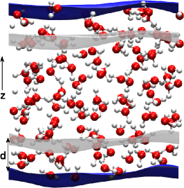
For the slab in the cuboid simulation box, we can get another surface by translating the surface along the system’s normal (into bulk) to a distance . The region between the two surfaces and is defined as the air-water interface. We have obtained HB dynamics at the instantaneous air-water interface, and there are two extreme cases to be considered.
III.1 Hydrogen bond dynamics based on interfacial molecule sampling
As the first method to obtain interface HB dynamics, we use molecule sampling at the instantaneous interface. Let be the time it takes for all water molecules in the simulation box to traverse the interface and bulk phase. If the trajectory length satisfies the condition , one finds time points , that are evenly spaced on the trajectory, then one obtains interface HB dynamics using the following procedure:
-
1.
For each observation time , define an interface with a thickness (see Fig. 1). Then, select a set of water molecules which are at the interface, and calculate the correlation functions , and through for the molecules that belong to the set .
-
2.
Determine average functions , and , of the correlation functions , and over sampling time points respectively.
-
3.
Determine reaction rate constant of breaking and reforming at the interface with thickness , by Eq. 4.
In the IMS method, since the configuration of molecules changes over time, the contribution of H-bonds in bulk phase is included. Therefore, the IMS method understimates the HB breaking rate constant of the interface.
III.2 Hydrogen bond dynamics based on interface HB population
After determining the instantaneous interface, we introduce an interface HB population operator as follows: It has a value 1 when a tagged molecular pair are H-bonded and both molecules are at the interface with a thickness , and 0 otherwise:
| (9) |
Then the correlation function that describes the fluctuation of H-bonds at the interface:
| (10) |
can be obtained.
Similar to Eq. 2 and Eq. 3, the corresponding correlation function
| (11) |
and interface reactive flux function
| (12) |
are obtained. The is 1 when the a tagged pair of water molecules , are at the interface and the interoxygen distance between the two molecules is less than at time , and 0 otherwise, i.e.,
| (16) |
Therefore, represents the prabability at time that a tagged pair of initially H-bonded water molecules at the interface are unbonded but remain at the interface and separated by less than ; measures the effective decay rate of H-bonds at the interface. The functions defined in Eq.s 10–12 are used to determine the reaction rate constant of breaking and reforming and the lifetimes of H-bonds at the interface by Eq. 4, in which , and are replaced by , and .
In the IHB method, it is accurate to choose the water molecules and H-bonds at the interface. However, for some special H-bonds, if it connects such two water molecules, one is at the interface and the other is in bulk water, the HB breaking reaction rate of such H-bonds will be artificially increased. Therefore, in contrast to the IMS method, the IHB method overestimates the HB breaking rate constant.
IV Discussions: effects of air-water interface on hydrogen bond dynamics
IV.1 Hydrogen bond relaxation
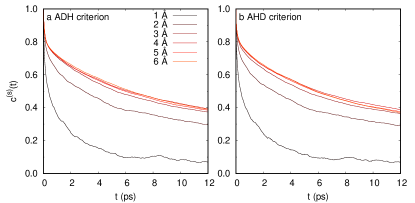
Two geometric criteria of H-bonds are used to calculate the , and the corresponding from Eq.10 are shown in Fig. 2. We find that as increases, at the interface relaxes more slowly. When is greater than 4 Å, recovers the bulk value. This feature is independent of the HB definition as shown by the comparison of results in panel a and b of Fig. 2.
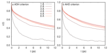
Figure 3 shows the -dependence of . Comparing Fig.s 2 and 3, we find that has the same feature: as increases, also relaxes more slowly; when is greater than 4 Å, also approaches a stable function. Comparing and , the second feature is that for the same , the value of is always slightly larger than . Moreover, regardless of the AHD or ADH criterion of H-bonds, these two features are valid. The first feature is the general one of interface H-bonds, while the second feature is derived from the difference in the definitions of HB population operators and . Using this difference between and , we can obtain the HB dynamics of the real interface, especially the thickness of the interface.
IV.2 Hydrogen bond breaking and reforming rate constants
We further examine how reaction rate constants and of H-bonds at the air-water interface vary with the interface thickness. Figure 4 compares the rate constants and the lifetime obtained by the IHB and IMS methods. We find that, for all the three quantities , and , the behavior as function of the thickness of the interface is hardly affected by the calculation methods. To illustrate this point more clearly, we compare the , and obtained under the two methods.

As shown in Fig. 4, when is larger than 4 Å, the constants and obtained by the two methods agree quantitatively.
The forward rate constant obtained by using the IHB method is relatively larger than that from the IMS method, and backward rate constant is relatively smaller. Since , this directly leads to a relatively shorter HB lifetime using the IHB method. This result is related to the definitions of and . The definition of makes the HB break rate at the interface artificially increased. The IMS method, which is based on , retains the original rate constant of H-bonds, but it may include the contribution of bulk water molecules to the rate constant.
In Fig. 4, the , and for the bulk water are also drawn with dashed lines as a reference. Comparing the above-mentioned physical quantities at the air-water interface and bulk water, we find that when the interface thickness is larger than 4 Å, no matter which statistical method is used, the obtained reaction rate constants of the interface water is greater than that in bulk water. Therefore, the HB lifetime in interface water is smaller than that in bulk water. Furthermore, as increases, and gradually close to the rates in bulk water at the same condition. These results are obtained by the least squares method in the same interval (0.2–12 ps). They show that the IHB method can get results as good as the IMS method when is larger than 4 Å.
The above two methods respectively give an extreme case of interface HB dynamics. In other words, the calculated HB dynamics obtained by IHB method is accelerated, compared to the real one. Real HB dynamics of the interface is between the results of the above two methods. Naturally, we approximate the true HB dynamics of the interface, by combining both the IHB and IMS methods. In these two extreme cases the interface HB characteriestics tends to be the same as the thickness of the interface increases. Properties such as the HB lifetime, HB reaction rate constants, and the thickness of the air-water interface can be estimated. For example, as the parameter increases, when all the , , of the interface calculated by both methods become consistent, the value of is the thickness of the air-water interface. The interface thickness value are comparable to those obtained experimentally (see Table B1). This result shows that our method of determining the interface thickness is reliable and expected to be used in more interface systems.
V Conclusions
Based on the DFTMD simulations, the IMS method partially gives information on the HB breaking and reforming reaction rate constants through the air-water interface and therefore partially shows how much the interface affects dynamics of H-bonds in water. The IHB method also provides partial information on the HB breaking and reforming reaction rates at the interface. As the thickness of interface increases, comparing results in the two extreme cases, we find that the HB breaking and reforming rate constants at the air-water interface tends to be uniform. Therefore, the real HB dynamical characteristics at the air-water interface can be derived. We conclude that from the perspective of HB dynamics, the thickness of the air-water interface at room temperature is 4 Å. In other words, at this thickness the HB dynamical properties of air-water interface become the same as bulk water.
The idea of combinating IHB and IMS can naturally be extended to the solution interfaces and other interfacial systems. For systems where statistical properties of the interface and bulk phase differ significantly, these differences will be represented more appropriately. In addition, the IHB method itself can also be generalize. For example, one can combine the HB population with the hydration shell of an ion, and then study the effects of ions through HB dynamics.
Appendix A Computational Methods
To describe the subtleties of H-bonding in water,Laasonen et al. (1993) we have performed DFTMD simulations Marx and Hutter (2000) for bulk water and the air-water interface. The simulations make use of some technologies that have been successfully tested on water and solutions,Khatib et al. (2016a, b); Khatib and Sulpizi (2017); Sulpizi et al. (2013) namely the Goedecker-Teter-Hutter (GTH) pseudopotentials,Goedecker, Teter, and Hutter (1996); Hartwigsen, Goedecker, and Hutter (1998); Krack (2005) Generalised Gradient Approximation (GGA) of the exchange-correlation functional,Becke (1988); Lee, Yang, and Parr (1988) and dispersion force correction, DFT-D3.Grimme et al. (2010); Klimeš and Michaelides (2012) By eliminating the strongly bound core electrons, the GTH pseudopotentials reduce the number of occupied electronic orbitals that have to be treated in an electronic structure calculation. There are dual-space Gaussian-type pseudopotentials that are separable and satisfy a quadratic scaling with respect to system size.Lu et al. (2019) The GGA functionals generally describe the dipole and quadruple moments of the molecules quite well; and DFT-D3 correction can treat the van der Waals dispersion forces in DFT and improve the structural properties without more computational cost, and thus can be used at the air-water interface.
The DFTMD calculation is implemented by a NVT code that implemented in the CP2K/QUICKSTEP package.VandeVondele et al. (2005); Kühne et al. (2020) The BLYP XC functional, which consists of Becke non-local exchangeBecke (1988) and Lee-Yang-Parr correlationLee, Yang, and Parr (1988) have been employed. The electron-ion interactions are described by GTH pseudopotentials.Hartwigsen, Goedecker, and Hutter (1998); Lippert, Hutter, and Parrinello (1999) A Gaussian basis for the wave functions and an auxiliary plane wave bisis set for the density are used in this scheme. DZVP-GTH basis set is used for all atoms and a cutoff of 280 Ry is chosen for the charge density.VandeVondele et al. (2005) The Nos-Hoover chain thermostatMartyna, Klein, and Tuckerman (1992) is used to conserve the temperature at 300 K. The simulation for the air-water interface use a time step of 0.5 fs.
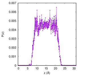
The bulk water system consisted of 128 water molecules in a periodic box of size Å3, and with a density of 1.00 g cm-3. The slab consisted of 128 water molecules in a periodic box of size Å3. The length of each trajectory in each simulation is ps. The RDFs and for the bulk water systems are shown in Fig. A1. The probability distribution of O and H atoms in the simulated model of air-water interface is showed in Fig. A2.

Appendix B The published values of the air-water interface thickness
| Method | (Å) | |
|---|---|---|
| Ellipsometry (Rayleigh) | 20∘C | 3.0 |
| Ellipsometry (Raman and Ramdas (1927)) | 20∘C | 5.0 |
| Ellipsometry (McBain, Bacon, and Bruce (1939)) | 20∘C | 2.26 |
| Ellipsometry (Kinosita and Yokota (1965)) | 20∘C | 7.1 |
| X-Ray Reflectivity(Braslau et al. (1988)) | 25 ∘C | 3.24 0.05 |
Acknowledgements.
G. H. acknowledges the financial support of the China Scholarship Council. The simulations were performed on the Mogon ZDV cluster in Mainz and on the Cray XE6 (Hermit) at the HRLS supercomputing center in Stuttgart.References
- Finlayson-Pitts and Jr. (2000) B. J. Finlayson-Pitts and J. N. P. Jr., Chemistry of the Upper and Lower Atmosphere: Theory, Experiments and Applications (Academic Press, San Diego, CA, 2000).
- Jungwirth and Tobias (2001) P. Jungwirth and D. J. Tobias, “Molecular Structure of Salt Solutions: A New View of the Interface with Implications for Heterogeneous Atmospheric Chemistry,” J. Phys. Chem. B 105, 10468–10472 (2001).
- Wilson et al. (2002) K. R. Wilson, R. D. Schaller, D. T. Co, R. J. Saykally, B. S. Rude, T. Catalano, and J. D. Bozek, “Surface relaxation in liquid water and methanol studied by x-ray absorption spectroscopy,” The Journal of Chemical Physics 117, 7738–7744 (2002), https://doi.org/10.1063/1.1508364 .
- Stiopkin et al. (2011) I. V. Stiopkin, C. Weeraman, P. A. Pieniazek, F. Y. Shalhout, J. L. Skinner, and A. V. Benderskii, “Hydrogen Bonding at the Water Surface Revealed by Isotopic Dilution Spectroscopy,” Nature 474, 192 (2011).
- Jeon et al. (2017) J. Jeon, C.-S. Hsieh, Y. Nagata, M. Bonn, and M. Cho, “Hydrogen bonding and vibrational energy relaxation of interfacial water: A full dft molecular dynamics simulation,” J. Chem. Phys. 147, 044707 (2017).
- Dang and Chang (1997a) L. X. Dang and T.-M. Chang, “Molecular dynamics study of water clusters, liquid, and liquid-vapour interface of water with many-body potentials,” J. Chem. Phys. 106, 8149 (1997a).
- Hsieh et al. (2013) C.-S. Hsieh, R. K. Campen, M. Okuno, E. H. G. Backus, Y. Nagata, and M. Bonn, “Mechanism of vibrational energy dissipation of free oh groups at the air-water interface,” Proceedings of the National Academy of Sciences 110, 18780–18785 (2013), https://www.pnas.org/doi/pdf/10.1073/pnas.1314770110 .
- Raman and Ramdas (1927) C. Raman and L. Ramdas, “On the thickness of the optical transition layer in liquid surfaces,” Phil. Mag. 3, 220 (1927).
- McBain, Bacon, and Bruce (1939) J. W. McBain, R. C. Bacon, and H. D. Bruce, “Optical surface thickness of pure water,” The Journal of Chemical Physics 7, 818–823 (1939), https://doi.org/10.1063/1.1750531 .
- Kinosita and Yokota (1965) K. Kinosita and H. Yokota, “Temperature dependence of the optical surface thickness of water,” J. Phys. Soc. Japan 20, 1086 (1965).
- Braslau et al. (1985) A. Braslau, M. Deutsch, P. S. Pershan, A. H. Weiss, J. Als-Nielsen, and J. Bohr, “Surface roughness of water measured by x-ray reflectivity,” Phys. Rev. Lett. 54, 114–117 (1985).
- Braslau et al. (1988) A. Braslau, P. S. Pershan, G. Swislow, B. M. Ocko, and J. Als-Nielsen, “Capillary waves on the surface of simple liquids measured by x-ray reflectivity,” Phys. Rev. A 38, 2457–2470 (1988).
- Superfine, Huang, and Shen (1991) R. Superfine, J. H. Huang, and Y. R. Shen, “Nonlinear Optical Studies of the Pure Liquid/Vapor Interface: Vibrational Spectra and Polar Ordering,” Phys. Rev. Lett. 66, 1066–1069 (1991).
- Ostroverkhov, Waychunas, and Shen (2005) V. Ostroverkhov, G. A. Waychunas, and Y. R. Shen, “New information on water interfacial structure revealed by phase-sensitive surface spectroscopy,” Phys. Rev. Lett. 94, 046102 (2005).
- Peng et al. (2021) Y. Peng, Z. Tong, Y. Yang, and C. Q. Sun, “The Common and Intrinsic Skin Electric-Double-Layer (EDL) and Its Bonding Characteristics of Nanostructures,” Applied Surface Science 539, 148208 (2021).
- Townsend, Gryko, and Rice (1985) R. M. Townsend, J. Gryko, and S. A. Rice, “Structure of the liquid–vapor interface of water,” J. Chem. Phys. 82, 4391–4392 (1985).
- Wilson, Pohorille, and Pratt (1987) M. A. Wilson, A. Pohorille, and L. R. Pratt, “Molecular dynamics of the water liquid-vapor interface,” J. Phys. Chem. 91, 4873–4878 (1987).
- Matsumoto and Kataoka (1988) M. Matsumoto and Y. Kataoka, “Study on liquid-vapor interface of water. i. simulational results of thermodynamic properties and orientational structure,” The Journal of Chemical Physics 88, 3233–3245 (1988), https://doi.org/10.1063/1.453919 .
- Townsend and Rice (1991) R. M. Townsend and S. A. Rice, “Molecular dynamics studies of the liquid-vapor interface of water,” The Journal of Chemical Physics 94, 2207–2218 (1991), https://doi.org/10.1063/1.459891 .
- Lie et al. (1993) G. C. Lie, S. Grigoras, L. X. Dang, D. Yang, and A. D. McLean, “Monte carlo simulation of the liquid–vapor interface of water using an ab initio potential,” The Journal of Chemical Physics 99, 3933–3937 (1993).
- Alejandre, Tildesley, and Chapela (1995) J. Alejandre, D. J. Tildesley, and G. A. Chapela, “Molecular dynamics simulation of the orthobaric densities and surface tension of water,” The Journal of Chemical Physics 102, 4574–4583 (1995).
- Taylor, Dang, and Garrett (1996) R. S. Taylor, L. X. Dang, and B. C. Garrett, “Molecular Dynamics Simulations of the Liquid/Vapor Interface of SPC/E Water,” J. Phys. Chem. 100, 11720–11725 (1996).
- Dang and Chang (1997b) L. X. Dang and T.-M. Chang, “Molecular dynamics study of water clusters, liquid, and liquid-vapor interface of water with many-body potentials,” The Journal of Chemical Physics 106, 8149–8159 (1997b), https://doi.org/10.1063/1.473820 .
- Beaglehole and Wilson (1993) D. Beaglehole and P. Wilson, “Thickness and Anisotropy of the Ice-Water Interface,” J. Phys. Chem. 97, 11053–11055 (1993).
- Sokhan and Tildesley (1997) V. P. Sokhan and D. J. Tildesley, “The free surface of water: molecular orientation, surface potential and nonlinear susceptibility,” Molecular Physics 92, 625–640 (1997).
- Morita and Hynes (2000) A. Morita and J. T. Hynes, “A theoretical analysis of the sum frequency generation spectrum of the water surface,” Chem. Phys. 258, 371–390 (2000).
- Paul and Chandra (2004) S. Paul and A. Chandra, “Hydrogen bond dynamics at vapour-water and metal-water interfaces,” Chemical Physics Letters 386, 218–224 (2004).
- Morita (2006) A. Morita, “Improved computation of sum frequency generation spectrum of the surface of water,” J. Phys. Chem. B 110, 3158–3163 (2006).
- Zhao et al. (2018) J. Zhao, G. Yao, S. B. Ramisetti, R. B. Hammond, and D. Wen, “Molecular dynamics simulation of the salinity effect on the n-decane/water/vapor interfacial equilibrium,” Energy Fuels 32, 11080–11092 (2018).
- Evans et al. (1993) R. Evans, J. Henderson, D. Hoyle, A. Parry, and Z. Sabeur, “Asymptotic decay of liquid structure: oscillatory liquid-vapour density profiles and the Fisher-Widom line,” Molecular Phys. 80, 755–775 (1993).
- Car and Parrinello (1985) R. Car and M. Parrinello, “Unified Approach for Molecular Dynamics and Density Functional Theory,” Phys. Rev. Lett. 55, 2471–2474 (1985).
- Marx and Hutter (2000) D. Marx and J. Hutter, “Ab Initio Molecular Dynamics: Theory and Implemention,” Modern Methods and Algorithms of Quantum Chemistry, J.Grotendorst (Ed.) John von Neumann Institute for Computing, Jülich, NIC Series 1, 301–499 (2000).
- Car (2002) R. Car, “Introduction to Density-Functional Theory and Ab-Initio Molecular Dynamics,” Quant. Struct. Act. Rel. 21, 97–104 (2002).
- Kuo and Mundy (2004) I.-F. W. Kuo and C. J. Mundy, “An Ab Initio Molecular Dynamics Study of the Aqueous Liquid-Vapor Interface,” Science 303, 658 (2004).
- Kühne et al. (2011) T. D. Kühne, T. A. Pascal, E. Kaxiras, and Y. Jung, “New Insights into the Structure of the Vapor/Water Interface from Large-Scale First-Principles Simulations,” J. Phys. Chem. Lett. 2, 105–113 (2011).
- Sulpizi et al. (2013) M. Sulpizi, M. Salanne, M. Sprik, and M.-P. Gaigeot, “Vibrational sum frequency generation spectroscopy of the water liquid-vapor interface from density functional theory-based molecular dynamics simulations,” J. Phys. Chem. Lett. 4, 83–87 (2013), http://dx.doi.org/10.1021/jz301858g .
- Khaliullin and Kühne (2013) R. Z. Khaliullin and T. D. Kühne, “Microscopic properties of liquid water from combined ab initio molecular dynamics and energy decomposition studies,” Phys. Chem. Chem. Phys. 15, 15746–15766 (2013).
- Pezzotti, Galimberti, and Gaigeot (2017) S. Pezzotti, D. R. Galimberti, and M.-P. Gaigeot, “2D H-Bond Network as the Topmost Skin to the Air-Water Interface,” J. Phys. Chem. Lett. 8, 3133–3141 (2017).
- Blas et al. (2001) F. J. Blas, E. M. D. Río, E. D. Miguel, and G. Jackson, “An examination of the vapour-liquid interface of associating fluids using a saft-dft approach,” Molecular Physics 99, 1851–1865 (2001).
- Willard and Chandler (2010) A. P. Willard and D. Chandler, “Instantaneous Liquid Interfaces,” J. Phys. Chem. B 114, 1954 (2010).
- Luzar and Chandler (1996) A. Luzar and D. Chandler, “Effect of environment on hydrogen bond dynamics in liquid water,” Phys. Rev. Lett. 76, 928–931 (1996).
- Chandra (2000) A. Chandra, “Effects of Ion Atmosphere on Hydrogen-Bond Dynamics in Aqueous Electrolyte Solutions,” Phys. Rev. Lett. 85, 768–771 (2000).
- Tarek and Tobias (2002) M. Tarek and D. J. Tobias, “Role of Protein-Water Hydrogen Bond Dynamics in the Protein Dynamical Transition,” Phys. Rev. Lett. 88, 138101 (2002).
- Pal, Bagchi, and Balasubramanian (2005) S. Pal, B. Bagchi, and S. Balasubramanian, “Hydration Layer of a Cationic Micelle, C10TAB: Structure, Rigidity, Slow Reorientation, Hydrogen Bond Lifetime, and Solvation Dynamics,” J. Phys. Chem. B 109, 12879–12890 (2005).
- Sciortino and Fornili (1989) F. Sciortino and S. L. Fornili, “Hydrogen Bond Cooperativity in Simulated Water: Time Dependence Analysis of Pair Interactions,” J. Chem. Phys. 90, 2786–2792 (1989).
- Soper and Phillips (1986) A. K. Soper and M. G. Phillips, “A New Determination of the Structure of Water at 25 ∘C,” Chem. Phys 107, 47–60 (1986).
- Teixeira, Bellisent-Funel, and Chen (1990) J. Teixeira, M. C. Bellisent-Funel, and S. H. Chen, “Dynamics of Water Studied by Neutron Scattering,” J. Phys. Condens. Matter 2, SA105 (1990).
- Luzar and Chandler (1993) A. Luzar and D. Chandler, “Structure and hydrogen bond dynamics of water-dimethyl sulfoxide mixtures by computer simulations,” J. Chem. Phys. 98, 8160–8173 (1993).
- Balasubramanian, Pal, and Bagchi (2002) S. Balasubramanian, S. Pal, and B. Bagchi, “Hydrogen-Bond Dynamics Near a Micellar Surface: Origin of the Universal Slow Relaxation at Complex Aqueous Interfaces,” Phys. Rev. Lett. 89, 115505 (2002).
- Chandler (1987) D. Chandler, Introduction to Morden Statistical Mechanics (Oxford University press, Oxford, 1987).
- Benjamin (2005) I. Benjamin, “Hydrogen Bond Dynamics at Water/Organic Liquid Interfaces,” J. Phys. Chem. B 109, 13711–13715 (2005).
- Rapaport (1983) D. C. Rapaport, “Hydrogen Bonds in Water: Network Organization and Lifetimes,” Mol. Phys. 50, 1151–1162 (1983).
- Luzar (2000) A. Luzar, “Resolving the Hydrogen Bond Dynamics Conundrum,” J. Chem. Phys. 113, 10663 (2000).
- Starr, Nielsen, and Sta (2000) F. W. Starr, J. K. Nielsen, and H. E. Sta, “Hydrogen-Bond Dynamics for the Extended Simple Point-Charge Model of Water,” Phys. Rev. E 62, 579–587 (2000).
- Chandler (1986) D. Chandler, “Roles of Classical Dynamics and Quantum Dynamics on Activated Processes Occurring in Liquids,” J. Stat. Phys. 42, 49–67 (1986).
- Chandler (1978) D. Chandler, “Statistical Mechanics of Isomerization Dynamics in Liquids and the Transition State Approximation,” J. Chem. Phys. 68, 2959–2970 (1978).
- Serva et al. (2018) A. Serva, S. Pezzotti, S. Bougueroua, D. R. Galimberti, and M.-P. Gaigeot, “Combining ab-initio and classical molecular dynamics simulations to unravel the structure of the 2d-hb-network at the air-water interface,” J. Molecular Structure 1165, 71–78 (2018).
- Laasonen et al. (1993) K. Laasonen, M. Sprik, M. Parrinello, and R. Car, “"ab initio" liquid water,” J. Chem. Phys. 99, 9080–9089 (1993), https://doi.org/10.1063/1.465574 .
- Khatib et al. (2016a) R. Khatib, E. H. G. Backus, M. Bonn, M. Perez-Haro, M.-P. Gaigeot, and M. Sulpizi, “Water Orientation and Hydrogen-Bond Structure at the Fluorite/Water Interface,” Scientific Reports 6, 24287 (2016a).
- Khatib et al. (2016b) R. Khatib, T. Hasegawa, M. Sulpizi, E. H. G. Backus, M. Bonn, and Y. Nagata, “Molecular Dynamics Simulations of SFG Librational Modes Spectra of Water at the Water-Air Interface,” J. Phys. Chem. C 120, 18665–18673 (2016b).
- Khatib and Sulpizi (2017) R. Khatib and M. Sulpizi, “Sum Frequency Generation Spectra from Velocity-Velocity Correlation Functions,” J. Phys. Chem. Lett. 8, 1310–1314 (2017).
- Goedecker, Teter, and Hutter (1996) S. Goedecker, M. Teter, and J. Hutter, “Separable dual-space gaussian pseudopotentials,” Phys. Rev. B 54, 1703–1710 (1996).
- Hartwigsen, Goedecker, and Hutter (1998) C. Hartwigsen, S. Goedecker, and J. Hutter, “Relativistic separable dual-space gaussian pseudopotentials from H to Rn,” Phys. Rev. B 58, 3641–3662 (1998).
- Krack (2005) M. Krack, “Pseudopotentials for H to Kr optimized for gradient-corrected exchange-correlation functionals,” Theor. Chem. Acc. 114, 145–152 (2005).
- Becke (1988) A. D. Becke, “Density-functional exchange-energy approximation with correct asymptotic behavior,” Phys. Rev. A 38, 3098 (1988).
- Lee, Yang, and Parr (1988) C. Lee, W. Yang, and R. G. Parr, “Development of the colic-salvetti correlation-energy formula into a functional of the electron density,” Phys. Rev. B 37, 785 (1988).
- Grimme et al. (2010) S. Grimme, J. Antony, S. Ehrlich, and H. Krieg, “A Consistent and Accurate Ab Initio Parametrization of Density Functional Dispersion Correction (DFT-D) for the 94 Elements H-Pu,” J. Chem. Phys. 132, 154104 (2010).
- Klimeš and Michaelides (2012) J. Klimeš and A. Michaelides, “Perspective: Advances and Challenges in Treating van der Waals Dispersion Forces in Density Functional Theory,” J. Chem. Phys. 137, 120901–120912 (2012).
- Lu et al. (2019) J.-B. Lu, D. C. Cantu, M.-T. Nguyen, J. Li, V.-A. Glezakou, and R. Rousseau, “Norm-Conserving Pseudopotentials and Basis Sets To Explore Lanthanide Chemistry in Complex Environments,” J. Chem. Theory Comput. 15, 5987–5997 (2019).
- VandeVondele et al. (2005) J. VandeVondele, M. Krack, F. Mohamed, M. Parrinello, T. Chassaing, and J. Hutter, “Quickstep: Fast and accurate density functional calculations using a mixed gaussian and plane waves approach,” Comput. Phys. Commun. 167, 103–128 (2005).
- Kühne et al. (2020) T. D. Kühne, M. Iannuzzi, M. Del Ben, V. V. Rybkin, P. Seewald, F. Stein, T. Laino, R. Z. Khaliullin, O. Schütt, F. Schiffmann, D. Golze, J. Wilhelm, S. Chulkov, M. H. Bani-Hashemian, V. Weber, U. Borštnik, M. Taillefumier, A. S. Jakobovits, A. Lazzaro, H. Pabst, T. Müller, R. Schade, M. Guidon, S. Andermatt, N. Holmberg, G. K. Schenter, A. Hehn, A. Bussy, F. Belleflamme, G. Tabacchi, A. Glöß, M. Lass, I. Bethune, C. J. Mundy, C. Plessl, M. Watkins, J. VandeVondele, M. Krack, and J. Hutter, “Cp2k: An electronic structure and molecular dynamics software package - quickstep: Efficient and accurate electronic structure calculations,” J. Chem. Phys. 152, 194103 (2020), https://doi.org/10.1063/5.0007045 .
- Lippert, Hutter, and Parrinello (1999) G. Lippert, J. Hutter, and M. Parrinello, “The gaussian and augmented-plane-wave density functional method for ab initio molecular dynamics simulations,” Theor. Chem. Acc. 103, 124 (1999).
- Martyna, Klein, and Tuckerman (1992) G. J. Martyna, M. L. Klein, and M. Tuckerman, “Nosé-hoover chains: The canonical ensemble via continuous dynamics,” J. Chem. Phys. 97, 2635 (1992).