Morphodynamics of Active Nematic Fluid Surfaces

Abstract

Morphodynamic equations governing the behaviour of active nematic fluids on deformable curved surfaces are constructed in the large deformation limit. Emphasis is placed on the formulation of objective rates that account for normal deformations whilst ensuring that tangential flows are Eulerian, and the use of the surface derivative (rather than the covariant derivative) in the nematic free energy, which elastically couples local order to out-of-plane bending of the surface. Focusing on surface geometry and its dynamical interplay with the hydrodynamics, several illustrative instabilities are then characterised. These include cases where the role of the Scriven-Love number and its nematic analogue are non-negligible, and where the active nematic forcing can be characterised by an analogue of the Föppl-von-Kármán number. For the former, flows and changes to the nematic texture are coupled to surface geometry by viscous dissipation. This is shown to result in non-trivial relaxation dynamics for a nematic tube. For the latter, the nematic active forcing couples to the surface bending terms of the nematic free energy, resulting in extensile (active ruffling) and contractile (active pearling) instabilities in the tube shape, as well as active bend instabilities in the nematic texture. In comparison to the flat case, such bend instabilities now have a threshold set by the extrinsic curvature of the tube. Finally, we examine a topological defect located on an almost flat surface and show that there exists a steady state where a combination of defect elasticity, activity and non-negligible spin-connection drive a shape change in the surface.

1 Introduction

Two dimensional fluid surfaces with nematic ordering are relevant for the characterisation of a variety of biological and soft matter systems, ranging from liquid crystal shells (Fernández-Nieves et al., 2007) to active composites of microtubules and kinesin motors at an oil-water interface (Sanchez et al., 2012). Of particular current interest is the increasing experimental evidence that nematic-like ordering plays a vital role in tissue mechanics (Saw et al., 2017) and morphogenesis (Maroudas-Sacks et al., 2021; Vafa & Mahadevan, 2022), where the interplay between topological defects and active forces control the morphology of protrusions and extrusions (Metselaar et al., 2019; Hoffmann et al., 2022).

Mathematically, the development of theory that couples hydrodynamics to surface geometry has lead to many interesting predictions on the role of viscous forces in the ordering and shaping of membranes in both isotropic (Sahu et al., 2020a; Arroyo & DeSimone, 2009; Hu et al., 2007; Tchoufag et al., 2022; Rangamani et al., 2013; Steigmann, 1999) and ordered fluids (Napoli & Vergori, 2016; Nestler & Voigt, 2022). Of particular note has been the inclusion of activity, leading to a variety of interesting morphodynamical phenomena and instabilities (Salbreux & Jülicher, 2017; Salbreux et al., 2022; Bächer et al., 2021; Khoromskaia & Salbreux, 2021; Hoffmann et al., 2022; Vafa & Mahadevan, 2022; Alert, 2022; Bell et al., 2022; Nestler & Voigt, 2022; Rank & Voigt, 2021) and even some attempts to construct rigorous shell theories of active materials (da Rocha et al., 2022). Much of this work has been driven by the desire to develop theories capable of describing the dynamics and morphogenesis of biological tissues and organisms (Al-Izzi & Morris, 2021; Jülicher et al., 2018).

Despite such interest, there is still a lack of formal characterisation regarding how geometry couples to dissipatve and active forces in nematic fluid surfaces. To this end, we develop a closed system of dynamical equations for nematic fluid surfaces in a similar manner to the approach taken in Arroyo & DeSimone (2009) for isotropic fluid membranes. We construct normal and tangential dissipative and reactive forces for the system subject to a free energy that depends only on surface geometry, the order parameter and its derivatives. We focus specifically on nematic liquid crystals in the one-constant limit of the Frank free energy and derive the general form of the so-called molecular field and the resulting normal forces for surfaces of arbitrary geometry (and vector ordering). Particular emphasis is placed on the formulation of objective rates that account for normal deformations whilst ensuring that tangential flows are Eulerian, and the use of the surface derivative (rather than the covariant derivative) in the nematic free energy, which elastically couples local order to out of plane bending of the surface. Given the increased interest in active interfaces, we also include an active Q-tensor term in the tangential stress tensor. From these equations we identify and discuss three dimensionless numbers which characterise regimes where there is a non-trivial interplay between geometry, dissipation and active forces.

To highlight how these numbers govern morphodynamics, we focus on some simple concrete examples. In the first case, we consider a tube with no activity (and uniformly ordered nematic parameter as a ground-state) and derive the relaxation dynamics for perturbations in the shape and order parameter. We then consider the case of active tubes, where we show that under active forces there are three characteristic types of instability depending on the value and sign of the activity (extensile vs contractile). Two of these instabilities are in the tube shape: contractile forces give an active pearling-like instability whose lengthscale is set by the bulk viscous time-scale, whilst extensile forces (above a threshold) lead to a ruffling instability whose lengthscale is set by the active stress. In addition, we find an instability in the texture that acts to drive spontaneous bend. This occurs for extensile activity in rod-like nematics, and for contractile activity in disk-like nematics. Interestingly, although similar to known spontaneous bend instabilities in flat geometries, the effects of curvature mean that the active forcing must exceed a finite threshold even in the infinite system size. Finally, we examine steady states in shape driven by active forcing of an almost flat surface in the presence of a topological defect and show that this leads to protrusions at the defect whose morphology is controlled by the activity. Specifically, increases in contractility lead to increased protrusion, whilst increases in extensility act to suppress protrusions.

2 A Theory of Deformable Nematic Fluid Surfaces

In this section, we construct a closed system of equations for the morphodynamics of nematic fluid surfaces (Fig. 1). In general, certain conventions from differential geometry will be adopted, such as the use of comma “,” and semicolon “;” subscripts to denote partial and covariant differentiation, respectively. For the uninitiated, a brief non-rigorous introduction to such notation is given in Appendix A. For a more complete treatment, we refer the reader to Needham (2021) and/or Frankel (2011).

Our starting point is a two-dimensional Riemannian manifold, $\mathcal{M}_{t}$, embedded in $\mathbb{R}^{3}$, and equipped with induced metric, $g_{\alpha\beta}$, and second fundamental form, $b_{\alpha\beta}$, where $\alpha,\beta\in\{1,2\}$ (and similarly for all Greek indices). The time-dependent position, $\bm{R}(u^{\alpha}(t),t)\in\mathbb{R}^{3}$, of each point $u\in\mathcal{M}_{t}$ implies a local velocity

$$\frac{\mathrm{d}\bm{R}}{\mathrm{d}t}=\bm{V}=v^{\alpha}\bm{e}_{\alpha}+v^{(n)}\bm{\hat{n}},$$ (1)

where the $\bm{e}_{\alpha}=\bm{R}_{,\alpha}$ are tangent to the surface at $\bm{R}$, and $\bm{\hat{n}}$ is the unit normal. To account for local order, each point is also associated with a vector $\bm{T}=T^{\alpha}\bm{e}_{\alpha}\in\mathcal{T}(\mathcal{M}_{t})$, referred-to as the director, which lives in the tangent bundle of the manifold.

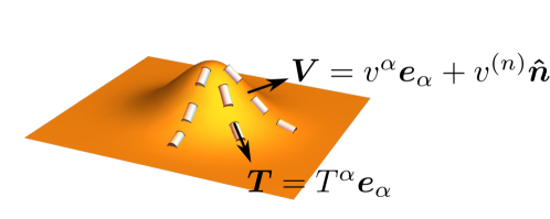
Figure 1: Schematic of a curved fluid surface with orientational order given by the director field $\bm{T}=T^{\alpha}\bm{e}_{\alpha}$ which moves with a velocity in $\mathbb{R}^{3}$ given by the vector field $\bm{V}=v^{\alpha}\bm{e}_{\alpha}+v^{(n)}\bm{\hat{n}}$.

Throughout, the fluid is assumed to be in the low Reynolds number regime and therefore inertial forces are neglected. As a result, the condition of force balance can be decomposed in the following way

$$\bm{f}^{e}+\bm{f}^{d}+\bm{f}^{bs}+\bm{f}^{c}+\bm{f}^{a}=0,$$ (2)

where $\bm{f}^{e}$ are elastic forces, $\bm{f}^{d}$ are dissipative forces, $\bm{f}^{bs}$ are broken symmetry forces, $\bm{f}^{c}$ are forces from constraints, and $\bm{f}^{a}$ are active forces.

We will also assume that the fluid is incompressible. As a result, the only dynamical equation in our theory, in addition to the trivial (1), is for the director field $T^{\alpha}$ on the surface. We write this as

$$\mathrm{D}_{t}T^{\alpha}=J^{\alpha}_{T}+J^{\alpha}_{c},$$ (3)

where $\mathrm{D}_{t}$ is the objective rate (calculated in the next section), $J^{\alpha}_{T}$ are dissipative currents resulting from an Onsager expansion/thermodynamic flux-force relation, and $J^{\alpha}_{c}$ is the current associated with the constraint of unit director magnitude.

2.1 Rate-of-deformation and vorticity tensors

A tensor of vital importance to fluid mechanics is the rate-of-deformation, or strain-rate tensor, $d_{\alpha\beta}$. The rate-of-deformation tensor is given by half of the time derivative of the metric on $\mathcal{M}_{t}$ [more formally, half of the Lie-derivative with respect to the flow, $\bm{V}$ (Arroyo & DeSimone, 2009; Marsden & Hughes, 1994)]. If we take the time derivative of the induced metric, $g_{\alpha\beta}=\bm{e}_{\alpha}\cdot\bm{e}_{\beta}$ as defined in (88), we find the following

$$\frac{\mathrm{d}g_{\alpha\beta}}{\mathrm{d}t}=\frac{\mathrm{d}\bm{e}_{\alpha}}{\mathrm{d}t}\cdot\bm{e}_{\beta}+\frac{\mathrm{d}\bm{e}_{\beta}}{\mathrm{d}t}\cdot\bm{e}_{\alpha}=\bm{V}_{,\alpha}\cdot\bm{e}_{\beta}+\bm{e}_{\alpha}\cdot\bm{V}_{,\beta}\text{.}$$ (4)

Substituting for $\bm{V}_{,\alpha}=\left(v^{\beta}{}_{;\alpha}-v^{(n)}b^{\beta}{}_{\alpha}\right)\bm{e}_{\beta}+\left(v^{\beta}b_{\alpha\beta}+v^{(n)}{}_{;\alpha}\right)\bm{\hat{n}}$ [see (A)] gives

$$d_{\alpha\beta}=\frac{1}{2}\frac{\mathrm{d}g_{\alpha\beta}}{\mathrm{d}t}=\frac{1}{2}\left(v_{\beta;\alpha}+v_{\alpha;\beta}\right)-v^{(n)}b_{\alpha\beta}\text{.}$$ (5)

Alternately, one can start from the expression for the rate-of-deformation tensor in $\mathbb{R}^{3}$ and project back onto the manifold $\mathcal{M}_{t}$

$$d_{\alpha\beta}\bm{e}^{\alpha}\otimes\bm{e}^{\beta}=\left[\frac{1}{2}\bm{V}_{,\alpha}\otimes\bm{e}^{\alpha}+\frac{1}{2}\left(\bm{V}_{,\alpha}\otimes\bm{e}^{\alpha}\right)^{\text{T}}\right]^{\bullet}\text{,}$$ (6)

where $(\cdot)^{\bullet}$ denotes projection onto $\mathcal{M}_{t}$ (i.e. contracting with tangent basis $\bm{e}_{\beta}$) which a quick calculation verifies gives the same result. Note that $\bm{V}\in\mathbb{R}^{3}$ but has support only on $\mathcal{M}_{t}$ and that the formal derivation of this requires some subtle constructions such as extensions of vector fields (Lee, 1997).

The vorticity tensor can be derived in an equivalent way giving an identical result to the flat geometry version

$$\Omega_{\alpha\beta}=\frac{1}{2}\left(v_{\beta;\alpha}-v_{\alpha;\beta}\right)\text{,}$$ (7)

which can be seen by noting that the terms of the asymmeterised deformation tensor proportional to $b_{\alpha\beta}$ vanish by symmetry under exchange of indices of the second fundamental form.

Here, we will consider incompressible fluids, the condition for which is that the rate-of-deformation tensor is traceless

$$d^{\alpha}{}_{\alpha}=\nabla_{\alpha}v^{\alpha}-2Hv^{(n)}=0\text{.}$$ (8)

In the absence of normal flows, this reproduces the classic incompressibility condition, $\nabla_{\alpha}v^{\alpha}=0$.

2.2 Objective rate of a vector field

The subject of objective rates is contentious in continuum mechanics, especially where changing geometry is concerned (Marsden & Hughes, 1994; Nitschke & Voigt, 2022). The challenge, in this case, is to ensure that tangential flows are Eulerian— i.e., coordinates are not advected with the flow— yet also properly account for out-of-plane surface dynamics, which are necessarily Lagrangian— i.e., coordinates are advected with surface movement (Waxman, 1984). We adopt a pragmatic approach, and choose a projected co-rotational rate. That is, we take the co-rotational derivative in $\mathbb{R}^{3}$ and project down onto the surface so as to recover the co-rotational objective rates for fixed-curved and flat surfaces, while still accounting for Lagrangian deformations of the surface in the normal direction.

For a vector field $\bm{T}$, which is confined to the tangent bundle of $\mathcal{M}_{t}$— i.e. $\bm{T}=T^{\alpha}\bm{e}_{\alpha}\in\mathcal{T}\left(\mathcal{M}_{t}\right)$— this takes the form

$$\text{D}_{t}\bm{T}^{\bullet}=\left[\frac{\mathrm{d}\bm{T}}{\mathrm{d}t}+\Omega\cdot\bm{T}\right]^{\bullet}=\left[\partial_{t}\bm{T}+v^{\alpha}\left(\bm{T}\right)_{,\alpha}+\Omega\cdot\bm{T}\right]^{\bullet}\text{.}$$ (9)

The first term is given by

$$\partial_{t}\bm{T} =\partial_{t}\left(T^{\alpha}\bm{e}_{\alpha}\right)=\partial_{t}T^{\alpha}\bm{e}_{\alpha}+T^{\alpha}\partial_{t}\bm{e}_{\alpha}$$

$$=\left(\partial_{t}T^{\alpha}-v^{(n)}T^{\beta}b_{\beta}{}^{\alpha}\right)\bm{e}_{\alpha}+T^{\alpha}v^{(n)}{}_{;\alpha}\bm{\hat{n}}\text{,}$$ (10)

where we have only included contributions from changing the basis vectors due to normal velocities, since we are in an Eulerian frame tangentially and therefore tangential velocities do not advect coordinates. The second term is given by

$$v^{\alpha}\nabla_{\alpha}\left(\bm{T}\right) =v^{\alpha}\left(T^{\beta}\bm{e}_{\beta}\right)_{,\alpha}=v^{\alpha}T^{\beta}{}_{;\alpha}\bm{e}_{\beta}+T^{\beta}v^{\alpha}b_{\alpha\beta}\bm{\hat{n}}\text{,}$$ (11)

and finally the third is simply given by

$$\Omega\cdot\bm{T}=\Omega^{\alpha}{}_{\beta}T^{\beta}\bm{e}_{\alpha}\text{.}$$ (12)

Putting this all together and projecting back onto the manifold gives

$$\text{D}_{t}T^{\alpha}= \partial_{t}T^{\alpha}+v^{\beta}T^{\alpha}{}_{;\beta}+\Omega^{\alpha}{}_{\beta}T^{\beta}-v^{(n)}T^{\beta}b_{\beta}{}^{\alpha}\text{,}$$ (13)

which is identical to the equivalent expression in flat geometry, with the exception of the final term.

To understand the origin of this term, consider a tube in cylindrical polar coordinates that is expanding outwards with velocity $v^{(n)}=\dot{R}$, where $R$ is the radius. There is no tangential flow, and the director field is assumed to be of constant magnitude in the $\bm{e}_{\theta}$ direction (i.e., $\bm{T}=T\bm{e}_{\theta}$). In this case, the second fundamental form has one non-zero component in the $\bm{e}_{\theta}$ direction. As a result, as $R$ increases, so does the size of the basis vector $\bm{e}_{\theta}$, and we require that $\mathrm{D}_{t}T^{\theta}=\partial_{t}T+\dot{R}T/R=0$ for the objective rate to be zero (fixed size for $\bm{T}$), which gives $T=T_{0}\exp(-\dot{R}/R)$.

2.3 Elastic forces

In general, we will consider surfaces with free energies of the following form

$$\mathcal{F}=\int_{\mathcal{M}_{t}}F\left(g_{\alpha\beta},b_{\alpha\beta},T_{\alpha}\right)\mathrm{d}A\text{,}$$ (14)

where $\mathrm{d}A=\sqrt{|g|}\mathrm{d}x^{1}\mathrm{d}x^{2}$ is the area element on the manifold. Whilst other free energies fit into this class, for example the tilt field of a lipid monolayer (Terzi & Deserno, 2017; Selinger et al., 1996), we will focus on the concrete example of the free energy of a nematic liquid crystal. Here, we will make use of standard descriptions of liquid crystals to define the molecular field as

$$h_{\alpha}=-\frac{\delta\mathcal{F}}{\delta T^{\alpha}}\text{,}$$ (15)

which we will make use of in order to derive the hydrodynamics of the ordered surface. The normal force given by varying the surface shape is then given by

$$\bm{f}_{\text{e}}=f^{\alpha}_{\text{e}}\bm{e}_{\alpha}+f^{(n)}_{\text{e}}\bm{\hat{n}}=-\frac{\delta\mathcal{F}}{\delta\bm{R}}\mathrm{.}$$ (16)

In the case of nematic liquid crystals, the one-constant approximation to the Frank free energy (Frank, 1958; DeGennes & Prost, 1993; Napoli & Vergori, 2012, 2016) is given by the following

$$\mathcal{F}^{\text{LC}}=\int_{\mathcal{M}_{t}}\frac{\mathcal{K}}{2}|\tilde{\nabla}_{s}\bm{T}|^{2}\mathrm{d}A\text{,}$$ (17)

where $\bm{T}=T^{\beta}\bm{e}_{\beta}$ is the nematic order parameter (we choose to use $T^{\beta}$ here rather than the usual $n^{\beta}$ in the nematic liquid crystal literature in order to avoid confusion with the surface normal vector $\bm{\hat{n}}$) on the tangent bundle $\mathcal{T}(\mathcal{M}_{t})$ and $\tilde{\nabla}_{s}$ is the surface derivative (not the covariant derivative) (Napoli & Vergori, 2012). The reason for our choice of the surface derivative, as opposed to the covariant derivative, is so as to correctly account for the bend due to extrinsic curvature. This is likely an important coupling for true active nematic surfaces, but is perhaps less relevant for nematic-like material surfaces such as epithelial tissues. The surface derivative can be written in terms of the covariant derivative and second fundamental form as follows

$$\tilde{\nabla}_{s}\bm{T}=\nabla_{\alpha}T^{\beta}\bm{e}^{\alpha}\otimes\bm{e}_{\beta}+T^{\beta}b_{\alpha\beta}\bm{e}^{\alpha}\otimes\hat{\bm{n}}\text{,}$$ (18)

and thus the full free energy is given by

$$\mathcal{F}^{\text{LC}}=\int_{\mathcal{M}_{t}}\frac{\mathcal{K}}{2}\left[\nabla_{\alpha}T^{\beta}\nabla^{\alpha}T_{\beta}+T^{\beta}T_{\gamma}b_{\alpha\beta}b^{\alpha\gamma}\right]\mathrm{d}A\text{.}$$ (19)

We will now compute the associated functional derivatives in the free energy rate ($\dot{\mathcal{F}}$). The functional derivative with respect to $T^{\alpha}$ gives the negative of the molecular field $h_{\alpha}$ as follows

$$\frac{\delta\mathcal{F}^{\text{LC}}}{\delta T^{\alpha}}=-h_{\alpha}=-\mathcal{K}\left[\Delta T_{\alpha}+\left(K\delta_{\alpha}^{\gamma}-2Hb_{\alpha}{}^{\gamma}\right)T_{\gamma}\right]\text{.}$$ (20)

We will make use of the rate formulas calculated in Appendix A to perform functional variations of the form

$$\delta g_{\alpha\beta}=\delta t\frac{\mathrm{d}}{\mathrm{d}t}\left(g_{\alpha\beta}\right)+O(\delta t^{2})\text{,}$$

$$\delta b_{\alpha\beta}=\delta t\frac{\mathrm{d}}{\mathrm{d}t}\left(b_{\alpha\beta}\right)+O(\delta t^{2})\text{,}$$

$$\delta\Gamma^{\gamma}_{\alpha\beta}=\delta t\frac{\mathrm{d}}{\mathrm{d}t}\left(\Gamma^{\gamma}_{\alpha\beta}\right)+O(\delta t^{2})\text{.}$$

Using this we find

$$\delta\mathcal{F}=\int_{\mathcal{M}_{t}}\frac{\mathcal{K}}{2}\Bigg{[}2\delta(\Gamma^{\beta}_{\alpha\mu})T^{\mu}g^{\alpha\gamma}g_{\beta\delta}T^{\delta}{}_{;\gamma}+T^{\beta}{}_{;\alpha}\delta(g^{\alpha\gamma})g_{\beta\delta}T^{\delta}{}_{;\gamma}+T^{\beta}{}_{;\alpha}g^{\alpha\gamma}\delta(g_{\beta\delta})T^{\delta}{}_{;\gamma}$$

$$+2\delta(b_{\alpha\beta})g^{\alpha\delta}b_{\delta\gamma}T^{\gamma}T^{\beta}+T^{\beta}T^{\gamma}b_{\alpha\beta}b_{\delta\gamma}\delta(g^{\alpha\delta})-2Hv^{(n)}\delta t\bigg{(}T^{\beta}{}_{;\alpha}T_{\beta}{}^{;\alpha}+T^{\beta}T_{\gamma}b_{\alpha\beta}b^{\alpha\gamma}\bigg{)}\Bigg{]}\mathrm{d}A\text{.}$$ (21)

Focusing purely on the normal variation we find

$$=\int_{\mathcal{M}_{t}}\mathcal{K}\delta t\Big{\{}\big{[}(v^{(n)}b_{\alpha}{}^{\gamma})_{;\beta}-(v^{(n)}b_{\alpha\beta})^{;\gamma}-(v^{(n)}b^{\gamma}{}_{\beta})_{;\alpha}\big{]}T^{\alpha}T^{\beta}{}_{;\gamma}+T^{\beta}{}_{;\alpha}T_{\beta;\gamma}b^{\alpha\gamma}v^{(n)}$$

$$-T^{\beta}{}_{;\alpha}T^{\gamma;\alpha}b_{\gamma\beta}v^{(n)}+(b^{\alpha}{}_{\gamma}T^{\gamma}T^{\beta})_{;\beta\alpha}v^{(n)}-T^{\gamma}T^{\beta}\big{(}2Hb_{\alpha\beta}b^{\alpha}{}_{\gamma}-Kb_{\beta\gamma}\big{)}v^{(n)}$$

$$+T^{\beta}T^{\gamma}b_{\alpha\beta}b_{\delta\gamma}b^{\alpha\delta}v^{(n)}-H\big{[}T^{\beta}{}_{;\alpha}T_{\beta}{}^{;\alpha}+T^{\beta}T_{\gamma}b_{\alpha\beta}b^{\alpha\gamma}\big{]}v^{(n)}\Big{\}}\mathrm{d}A\text{.}$$ (22)

Notice that the first terms from the variation of the covariant derivative include derivatives in the normal velocity. Integrating these by parts and pushing terms to the boundary we can find the following functional variation in the bulk of the surface

$$\delta\mathcal{F}= \int_{\mathcal{M}_{t}}\mathcal{K}v^{(n)}\delta t\Big{\{}b_{\alpha\beta}(T^{\alpha}T^{\beta}{}_{;\gamma})^{;\gamma}+b^{\gamma}{}_{\beta}(T^{\alpha}T^{\beta}{}_{;\gamma})_{;\alpha}-b_{\alpha}{}^{\gamma}(T^{\alpha}T^{\beta}{}_{;\gamma})_{;\beta}+T^{\beta}{}_{;\alpha}T_{\beta;\gamma}b^{\alpha\gamma}$$

$$-T^{\beta}{}_{;\alpha}T^{\gamma;\alpha}b_{\gamma\beta}+(b^{\alpha}{}_{\gamma}T^{\gamma}T^{\beta})_{;\beta\alpha}-T^{\gamma}T^{\beta}\big{(}2Hb_{\alpha\beta}b^{\alpha}{}_{\gamma}-Kb_{\beta\gamma}\big{)}+T^{\beta}T^{\gamma}b_{\alpha\beta}b_{\delta\gamma}b^{\alpha\delta}$$

$$-H\big{[}T^{\beta}{}_{;\alpha}T_{\beta}{}^{;\alpha}+T^{\beta}T_{\gamma}b_{\alpha\beta}b^{\alpha\gamma}\big{]}\Big{\}}\mathrm{d}A+\text{Boundary Terms}\text{.}$$ (23)

From this, and noting that the second and third terms cancel due to symmetry of $T^{\alpha}T^{\beta}$ and $b_{\alpha\beta}$, we find the forces in the normal direction from the free energy as the following

$$f^{(n)}_{\text{e}}=-\mathcal{K}\Big{\{}b_{\alpha\beta}(T^{\alpha}T^{\beta}{}_{;\gamma})^{;\gamma}+T^{\beta}{}_{;\alpha}\left(T_{\beta;\gamma}b^{\alpha\gamma}-T^{\gamma;\alpha}b_{\gamma\beta}\right)+(b^{\alpha}{}_{\gamma}T^{\gamma}T^{\beta})_{;\beta\alpha}$$

$$-T^{\gamma}T^{\beta}\big{(}2Hb_{\alpha\beta}b^{\alpha}{}_{\gamma}-Kb_{\beta\gamma}\big{)}+T^{\beta}T^{\gamma}b_{\alpha\beta}b_{\delta\gamma}b^{\alpha\delta}-H\big{[}T^{\beta}{}_{;\alpha}T_{\beta}{}^{;\alpha}+T^{\beta}T_{\gamma}b_{\alpha\beta}b^{\alpha\gamma}\big{]}\Big{\}}\text{.}$$ (24)

Note that the third term gives forces which go like the second derivative of the curvature tensor, but traced out along the directions of the nematic order parameter. Such a term is essentially an anisotropic bending rigidity that would not be found in the case where the covariant derivative, rather than surface derivative, was used in the free energy (Napoli & Vergori, 2012; Santiago et al., 2019; Santiago & Monroy, 2020). This gives significantly different equations to many of those currently analysed in the literature; both equilibrium and dynamical (Frank & Kardar, 2008; Salbreux et al., 2022; Hoffmann et al., 2022; Santiago, 2018).

Similarly for the tangential variations we find the following elastic force

$$f^{\alpha}_{\text{e}}=-\frac{\mathcal{K}}{2}\bigg{\{} \left(T^{\beta}T^{\alpha;\gamma}\right)_{;\beta\gamma}+\left(T_{\beta;\gamma}T^{\beta;\alpha}\right)^{;\gamma}-\left(T_{\beta;\gamma}T^{\alpha;\gamma}\right)^{;\beta}-2\left(b^{\alpha}{}_{\beta}b^{\gamma}{}_{\mu}T^{\mu\beta}\right)_{;\gamma}$$

$$-2\left(b^{\gamma}{}_{\mu}T^{\mu\beta}\right)_{;\beta}b^{\alpha}{}_{\gamma}+\left(T^{\beta}T^{\gamma}b_{\mu\beta}b^{\alpha}{}_{\gamma}\right)^{;\mu}\bigg{\}}\text{.}$$ (25)

This is essentially a generalised version of the Ericksen force (DeGennes & Prost, 1993). For simplicity we will neglect this tangential component in our later examples as it leaves the phenomenology of the equations unchanged. This approximation is taken in many exact calculations in active hydrodynamics (Hoffmann et al., 2022; Giomi et al., 2014; Kruse et al., 2004; Edwards & Yeomans, 2009), however in principle this term should be included in full non-linear solutions.

2.4 Surface Tension and Director Constraints

We consider two constraints upon our system whose contributions to the dynamical equations can generically be derived from a Rayleigh dissipation functional (DeGennes & Prost, 1993; Doi, 2011). However, we avoid a full variational treatment here for the sake of brevity and instead simply state the contributions whose derivation can be found elsewhere (DeGennes & Prost, 1993; Arroyo & DeSimone, 2009; Marchetti et al., 2013).

The first constraint is that of constant area, or incompressibility, which is expressed by (8). The corresponding Lagrange multiplier is the surface tension, $\zeta$, which acts isotropically via stresses $\sigma^{(st)}_{\alpha\beta}=\zeta g_{\alpha\beta}$. Taking the surface divergence of $\sigma^{(st)}$ gives the following contribution to the force balance condition

$$\bm{f}^{\text{c}}=\nabla^{\alpha}\zeta\bm{e}_{\alpha}+2H\zeta\bm{\hat{n}}\text{.}$$ (26)

The second constraint is to fix the magnitude of the nematic director (DeGennes & Prost, 1993). This is achieved by imposing

$$T_{\alpha}\mathrm{D}_{t}T^{\alpha}=0\text{,}$$ (27)

which implies $T^{\alpha}T_{\alpha}=\text{constant}$, with the constant specified by the initial conditions on $T^{\alpha}$ (Kruse et al., 2005). The associated Lagrange multiplier we label by $\lambda$, and the corresponding contribution to the director current (Prost et al., 2015) is just

$$J^{\alpha}_{c}=-\lambda T^{\alpha}\text{.}$$ (28)

This term can be viewed from a variational perspective as either a constraint on the Rayleigh dissipation functional of the form, $\int\lambda T_{\alpha}\mathrm{D}_{t}T^{\alpha}\mathrm{d}A$, or a contribution to the molecular field from a constraint on the free energy of the form, $\int\frac{1}{2}\lambda\gamma T_{\alpha}T^{\alpha}\mathrm{d}A$ (DeGennes & Prost, 1993).

2.5 Constitutive Relation and Dissipative Forces

The viscous stress tensor in the tangent bundle is given as an Onsager expansion (Doi, 2011; DeGennes & Prost, 1993) in the thermodynamic fluxes. At lowest non-trivial order, it is given by

$$\sigma_{\alpha\beta}=2\eta d_{\alpha\beta}+\frac{\nu}{2}\left(T_{\alpha}h_{\beta}+T_{\beta}h_{\alpha}\right)\text{,}$$ (29)

where $h_{\alpha}$ is the molecular field (20), $d_{\alpha\beta}$ the rate-of-deformation tensor, $\eta$ is the shear viscosity and $\nu$ the spin connection coefficients of the vector field (essentially the ratio of anisotropic viscosity to isotropic viscosity (DeGennes & Prost, 1993)). Here stable solutions require $|\nu|>1$, with $\nu<-1$ corresponding to rod-like nematics and $\nu>1$ to disk-like nematics (Edwards & Yeomans, 2009; Marchetti et al., 2013). Note that, as we only consider incompressible fluids, we discard the bulk viscosity terms and associated spin connections (DeGennes & Prost, 1993). The dissipative forces on our surface are then given as

$$\bm{f}^{\text{d}}=\nabla_{\beta}\sigma^{\alpha\beta}\bm{e}_{\alpha}+\sigma^{\alpha\beta}b_{\alpha\beta}\bm{\hat{n}}\text{.}$$ (30)

For the terms in the tangent bundle we find the following

$$\nabla_{\beta}\sigma^{\alpha\beta}=2\eta d^{\alpha\beta}{}_{;\beta}+\frac{\nu}{2}\left(T^{\alpha}h^{\beta}+T^{\beta}h^{\alpha}\right)_{;\beta}\text{,}$$ (31)

where we can unpack the first term to

$$2\eta d^{\alpha\beta}{}_{;\beta}=\eta\left(v^{\alpha;\beta}+v^{\beta;\alpha}-2v^{(n)}b^{\alpha\beta}\right)_{;\beta}=\eta\Delta v^{\alpha}+\eta v^{\beta}{}_{;\alpha\beta}-2\eta\left(v^{(n)}b^{\alpha\beta}\right)_{;\beta}\text{,}$$ (32)

where $\Delta=\nabla_{\alpha}\nabla^{\alpha}$ is the Bochner Laplacian. By making use of the Codazzi equation, (96), and contracted Gauss Equation, (99) we find

$$2\eta d^{\alpha\beta}{}_{;\beta}=\eta\bigg{[}\Delta v^{\alpha}-2\left(v^{(n)}H\right)^{;\alpha}+Kv^{\alpha}+2\left(2Hg^{\alpha\beta}-b^{\alpha\beta}\right)v^{(n)}{}_{;\beta}\bigg{]}\text{.}$$ (33)

Thus the tangential forces are given by

$$\sigma^{\alpha\beta}{}_{;\beta}= \frac{\nu}{2}\left(T^{\alpha}h^{\beta}+T^{\beta}h^{\alpha}\right)_{;\beta}$$

$$+\eta\bigg{[}\Delta v^{\alpha}-2\left(v^{(n)}H\right)^{;\alpha}+Kv^{\alpha}+2\left(2Hg^{\alpha\beta}-b^{\alpha\beta}\right)v^{(n)}{}_{;\beta}\bigg{]}\text{.}$$ (34)

The normal forces are given by contracting the stress tensor with the second fundamental form

$$\sigma^{\alpha\beta}b_{\alpha\beta}=2\eta b^{\alpha\beta}v_{\beta;\alpha}-4\eta\left(2H^{2}-K\right)v^{(n)}+\nu T^{\alpha}h^{\beta}b_{\alpha\beta}\text{.}$$ (35)

2.6 Broken Symmetry Terms

We can also include broken symmetry terms in the stress tensor which contribute nothing to the overall dissipation as their dynamics are associated with Goldstone modes in the system, hence the name “Broken Symmetry” (DeGennes & Prost, 1993; Kruse et al., 2005). For vector fields these contribute an anti-symmetric part to the stress tensor of the following form

$$\sigma^{(bs)}_{\alpha\beta}=\frac{1}{2}\left(T_{\alpha}h_{\beta}-T_{\beta}h_{\alpha}\right)\text{.}$$ (36)

Note that these terms only contribute to the tangential forces as they vanish in the normal due to the symmetry of the second fundamental form upon index relabelling. The broken symmetry forces are thus given by

$$\bm{f}^{bs}=\nabla_{\beta}\sigma^{(bs)\alpha\beta}\bm{e}_{\alpha}+\sigma^{(bs)\alpha\beta}b_{\alpha\beta}\bm{\hat{n}}=\frac{1}{2}\left(T^{\alpha}h^{\beta}-T^{\beta}h^{\alpha}\right)_{;\beta}\bm{e}_{\alpha}\text{.}$$ (37)

2.7 Director Terms

Expanding out in an Onsager fashion for the director rate in terms of nematic relaxation, we find the following couplings

$$J^{\alpha}_{T}=\gamma^{-1}h^{\alpha}-\nu d^{\alpha}{}_{\beta}T^{\beta}\text{,}$$ (38)

which gives terms in a similar manner to the flat case (Kruse et al., 2005). Note that the constant $\nu$ is the same as for the director terms in the stress tensor by the Onsager reciprocal relations. Adding this together with the constraint current, (28), gives the full Onsager expansion for the director rate as

$$\mathrm{D}_{t}T^{\alpha}=\gamma^{-1}h^{\alpha}-\nu d^{\alpha}{}_{\beta}T^{\beta}-\lambda T^{\alpha}\text{.}$$ (39)

2.8 Active Terms

We consider a simple extension to the tangential stress tensor that represent the dipolar-like active forces that are characteristic of many active nematic systems (Sanchez et al., 2012; Marchetti et al., 2013). For a detailed introduction to active matter we refer the reader to the following reviews (Marchetti et al., 2013; Ramaswamy, 2017) and for active liquid crystals in particular to (Doostmohammadi et al., 2018).

Active liquid crystals have generated significant interest in recent years due to several experimental realisations (Sanchez et al., 2012; Keber et al., 2014) which have revealed the fascinating interplay between active stresses and geometry of the director, particularly in the coupling of geometry of the surfaces to the dynamics of topological defects (Giomi et al., 2014; Pearce et al., 2019; Pearce, 2020; Khoromskaia & Alexander, 2017). In addition such systems have been suggested as minimal models for tissues (Blanch-Mercader et al., 2021b, a) and the actomyosin cell cortex (Kruse et al., 2005).

Here, we consider the standard form for the active nematic stress tensor:

$$\sigma^{\text{(a)}}_{\alpha\beta}=\Sigma Q_{\alpha\beta}=\Sigma\left(T_{\alpha}T_{\beta}-\frac{1}{2}g_{\alpha\beta}\right)\text{.}$$ (40)

For $\Sigma>0$ such stresses are contractile in nature and for $\Sigma<0$ they are extensile. This form represents the simplest form of anisotropic active stress, however more complicated couplings are possible (Salbreux et al., 2022; Salbreux & Jülicher, 2017; Naganathan et al., 2014). The active forces from (40) are given by

$$\bm{f}^{a}=\sigma^{\text{(a)}\alpha\beta}{}_{;\beta}\bm{e}_{\alpha}+\sigma^{\text{(a)}\alpha\beta}b_{\alpha\beta}\bm{\hat{n}}\text{.}$$ (41)

2.9 Full Dynamical Equations

Putting together all our force balance terms, constraints and polarisation currents gives the following system, which are essentially ordered fluid versions of the equations derived for isotropic fluid membranes in Arroyo & DeSimone (2009).

Polarisation dynamics:

$$\mathrm{D}_{t}T^{\alpha}=\gamma^{-1}h^{\alpha}-\nu d^{\alpha}{}_{\beta}T^{\beta}-\lambda T^{\alpha}\text{,}$$ (42)

Tangential force balance:

$$\frac{1}{2}\left(T^{\alpha}h^{\beta}-T^{\beta}h^{\alpha}\right)_{;\beta}+\eta\bigg{[}\Delta v^{\alpha}-2\left(v^{(n)}H\right)^{;\alpha}+Kv^{\alpha}+2\left(2Hg^{\alpha\beta}-b^{\alpha\beta}\right)v^{(n)}{}_{;\beta}\bigg{]}$$

$$\quad\quad+\frac{\nu}{2}\left(T^{\alpha}h^{\beta}+T^{\beta}h^{\alpha}\right)_{;\beta}+f^{\alpha}_{\text{e}}+\zeta^{;\alpha}+\sigma^{\text{(a)}\alpha\beta}{}_{;\beta}=0\text{,}$$ (43)

Normal force balance:

$$2\eta b^{\alpha\beta}v_{\beta;\alpha}-4\eta\left(2H^{2}-K\right)v^{(n)}+\nu T^{\alpha}h^{\beta}b_{\alpha\beta}+2H\zeta+f^{(n)}_{\text{e}}+\sigma^{\text{(a)}\alpha\beta}b_{\alpha\beta}=0\text{,}$$ (44)

Constraint equations (constant director and incompressibility):

$$T_{\alpha}\mathrm{D}_{t}T^{\alpha}=0;\quad v^{\alpha}{}_{;\alpha}-2Hv^{(n)}=0\text{,}$$ (45)

Closure between surface velocity and geometry:

$$\bm{V}=\frac{\mathrm{d}\bm{R}}{\mathrm{d}t}\text{.}$$ (46)

2.10 Dimensionless Numbers

There is an interesting point to make regarding the normal force balance equation. It contains the term $\eta b^{\alpha\beta}v_{\beta;\alpha}$, which describes the curvature induced coupling between viscous forces and shape. Such couplings have been discussed extensively for isotropic fluid membranes (Sahu et al., 2020a; Al-Izzi et al., 2020a). These phenomena can be understood in terms of the dimensionless Scriven-Love number (Scriven, 1960)

$$\text{SL}=\frac{O(\eta b^{\alpha\beta}v_{\beta;\alpha})}{O(\text{Bending Forces})}=\frac{\eta VL}{\mathcal{K}}\text{,}$$ (47)

where $V$ and $L$ are characteristic velocities and length-scales and we have assumed that $\text{Bending Forces}\sim\mathcal{K}L^{-3}$ (i.e., like the bending energy and Laplacian of the mean curvature).

In addition, however, there is a new anisotropic coupling due to terms $\sim\nu T^{\alpha}h^{\beta}b_{\alpha\beta}$ which, when compared to bending forces, could be thought of as a “Liquid Crystalline Scriven-Love Number”:

$$\text{SL}^{(LC)}=\frac{O(\nu T_{\alpha}h_{\beta}b^{\alpha\beta})}{O(\text{Bending Forces})}=\nu\text{.}$$ (48)

As such, the dimensionless number associated with out of plane liquid crystalline dissipative forces is just the spin connection coefficient, $\nu$.

In addition to this, there is also the dimensionless active stress. As this is a number comparing tangential stress to bending stress, we can consider it as an analogue of the Föppl-von-Kármán number, Y, that would typically compare stretching to bending forces in passive shell theory (Audoly & Pomeau, 2010). In our case, this is given by

$$\text{Y}^{(\text{Active})}=\frac{\Sigma L^{2}}{\mathcal{K}}\text{.}$$ (49)

Note that this implies that in highly curved geometries bending forces will suppress active deformations.

3 Applications

To illustrate the potential interplay between geometry, ordering and flow, we provide some concrete examples. We focus first on the case where activity is not present, but where the highly curved geometry of a tube leads to couplings between the director and shape that are not present in the flat or close-to-flat cases studied in (Salbreux et al., 2022). We then consider the ways in which active anisotropic stresses can drive tubes unstable, before finally considering the effects of activity on a topological defect located at the centre of a close to flat sheet.

3.1 Relaxation dynamics about a perturbed tube

We start with a simple example of a tube of radius $r(\theta,z,t)=r+\epsilon u(\theta,z,t)$, where $\epsilon$ is some dimensionless parameter that will be considered small. Such tubes have been shown in the case of isotropic membranes to have non-negligible Scriven-Love effects (Sahu et al., 2020a). The surface is prescribed by the vector $\bm{R}=(r\cos\theta,r\sin\theta,z)$. We can thus calculate the induced basis and metric

$$[g_{\alpha\beta}]=\left(\begin{matrix}r(r+2\epsilon u)&0\\ 0&1\end{matrix}\right)+O(\epsilon^{2})\text{,}$$ (50)

and the second fundamental form

$$[b_{\alpha\beta}]=\left(\begin{matrix}\epsilon u_{,\theta\theta}-\epsilon u-r&\epsilon u_{,\theta z}\\ \epsilon u_{,\theta z}&\epsilon u_{,zz}\end{matrix}\right)+O(\epsilon^{2})\text{.}$$ (51)

This gives mean and Gaussian curvature to first order as

$$H=\frac{\epsilon}{2}\left(u_{,zz}+\frac{1}{r^{2}}u_{,\theta\theta}+\frac{1}{r^{2}}u\right)-\frac{1}{2r}\text{,}$$ (52)

$$K=-\frac{\epsilon u_{,zz}}{r}\text{.}$$ (53)

We write the director field as $\bm{T}=\frac{\epsilon T^{\theta}}{r}\bm{e}_{\theta}+(1+\epsilon T^{z})\bm{e}_{z}+O(\epsilon^{2})$, where we have chosen the $O(1)$ term to be the unit vector in the $z$ direction such that the molecular field vanishes for the unperturbed state (Napoli & Vergori, 2012). Thus, at lowest order, the constraint equation on director unity becomes

$$\partial_{t}T^{z}=0\text{,}$$ (54)

and all the dynamics are in the $\theta$ direction, i.e. perpendicular to the initial zeroth order nematic ordering, as one would expect for the perturbative dynamics of a unit vector field. The velocity we write as $\vec{V}=\epsilon(v^{\theta}/r\bm{e}_{\theta}+v^{z}\bm{e}_{z}+\partial_{t}u\bm{\hat{n}})$ and so the continuity equation becomes

$$\frac{\partial_{t}u}{r}+\frac{v^{\theta}_{,\theta}}{r}+v^{z}_{,z}=0\text{.}$$ (55)

The molecular field is given by

$$h^{\alpha}\bm{e}_{\alpha}= \mathcal{K}\epsilon\left(T^{\theta}_{,zz}+\frac{1}{r^{2}}T^{\theta}_{,\theta\theta}-\frac{1}{r^{2}}T^{\theta}+\frac{2}{r^{2}}u_{,\theta z}\right)\frac{1}{r}\bm{e}_{\theta}+\mathcal{K}\epsilon\left(\frac{T^{z}_{,\theta\theta}}{r^{2}}+T^{z}_{,zz}\right)\bm{e}_{z}\text{,}$$ (56)

and can be substituted to then find the polarization rate equation whose components are given by

$$\bm{e}_{\theta}:\quad\epsilon\Bigg{[}-\frac{\mathcal{K}}{\gamma r}\left(T^{\theta}_{,zz}+\frac{T^{\theta}_{,\theta\theta}}{r^{2}}-\frac{T^{\theta}}{r^{2}}+2\frac{u_{,\theta z}}{r^{2}}\right)+\frac{1}{r}\left(\partial_{t}T^{\theta}+\frac{1}{2}v^{\theta}_{,z}+\frac{1}{2r}v^{z}_{,\theta}\right)$$

$$\quad\quad\quad+\frac{1}{r}\left(\lambda T^{\theta}+\frac{\nu}{2}v^{\theta}_{,z}+\frac{\nu}{2r}v^{z}_{,\theta}\right)\Bigg{]}=0\text{,}$$ (57)

$$\bm{e}_{z}:\quad\lambda-\epsilon\left[\frac{\mathcal{K}}{\gamma}\left(\frac{1}{r^{2}}T^{z}_{,\theta\theta}+T^{z}_{,zz}\right)+\partial_{t}T^{z}+\lambda T^{z}+\nu v^{z}_{,z}\right]=0\text{.}$$ (58)

The modified covariant Stokes equation (tangential force balance) is given component-wise by

$$\bm{e}_{\theta}:\quad\frac{\zeta_{,\theta}(r-2\epsilon u)}{r^{3}}+\frac{\mathcal{K}(\nu-1)\epsilon}{2r^{3}}\left(r^{2}T^{\theta}_{,zzz}-T^{\theta}_{,z}+T^{\theta}_{,\theta\theta z}+2u_{,\theta zz}\right)$$

$$\quad\quad\quad+\frac{\eta\epsilon}{r^{3}}\left(r^{2}v^{\theta}_{,zz}+\partial_{t}u_{,\theta}+v^{\theta}_{,\theta\theta}\right)=0\text{,}$$ (59)

$$\bm{e}_{z}:\quad\frac{\eta\epsilon}{r^{2}}\left(r^{2}v^{z}_{,zz}-r\partial_{t}u_{,z}+v^{z}_{,\theta\theta}\right)+\zeta_{,z}=0\text{.}$$ (60)

The normal components of force due to the liquid crystal free energy are more complicated to calculate, however. Nevertheless, at $O(\epsilon)$ only the third term of (2.3) contributes, giving

$$\left(b^{\alpha}{}_{\gamma}T^{\gamma}T^{\beta}\right)_{;\beta\alpha}=\epsilon\left[u_{,zzzz}-\frac{1}{r^{2}}T^{\theta}_{,z\theta}+\frac{1}{r^{2}}u_{,zz\theta\theta}\right]+O(\epsilon^{2})\text{,}$$ (61)

which gives the following shape equation

$$\frac{\mathcal{K}\epsilon}{r^{2}}\left(r^{2}u_{,zzzz}-T^{\theta}_{z\theta}+u_{,zz\theta\theta}\right)-\frac{\zeta}{r^{2}}\left[\epsilon\left(r^{2}u_{,zz}+u_{,\theta\theta}+u\right)-r\right]$$

$$\quad\quad+\frac{2\eta\epsilon}{r^{2}}\left(\partial_{t}u+v^{\theta}_{,\theta}\right)=0\text{.}$$ (62)

Taking the case where $\epsilon=0$ we find a ground state with

$$\lambda=0\text{,}$$ (63)

$$\zeta=0\text{,}$$ (64)

$$\bm{T}=\bm{e}_{z}\text{,}$$ (65)

as required. Note that as the bending energy term is anisotropic it gives no characteristic lengthscale of the tube as compared to the case of a lipid bilayer, for example, where the groundstate radius of the tube is set by the ratio of isotropic bending energy to surface tension ($r_{0}=\sqrt{\kappa/2\zeta}$) (Zhong-Can & Helfrich, 1989; Nelson et al., 1995; Gurin et al., 1996; Powers, 2010; Boedec et al., 2014; Fournier & Galatola, 2007).

We now take $\zeta=\epsilon\zeta$, $\lambda=\epsilon\lambda$ and, take the Fourier transform in space $\bar{f}_{q,m}=(1/4\pi^{2})\int\mathrm{d}z\mathrm{d}\theta f(z,\theta)e^{-\dot{\imath}m\theta-\dot{\imath}qz}$. Using each of (54), (55), (3.1), (3.1) & (3.1), leaves simply two dynamical equations for $\bar{u}_{qm}$ and $\bar{T}^{\theta}_{qm}$ which are given in dimensionless form as follows

$$\partial_{\tilde{t}}\left(\begin{matrix}\bar{T}^{\theta}_{qm}\\ \bar{u}_{qm}\end{matrix}\right)=A\cdot\left(\begin{matrix}\bar{T}^{\theta}_{qm}\\ \bar{u}_{qm}\end{matrix}\right)=\left(\begin{matrix}A_{11}&A_{12}\\ A_{21}&A_{22}\end{matrix}\right)\cdot\left(\begin{matrix}\bar{T}^{\theta}_{qm}\\ \bar{u}_{qm}\end{matrix}\right)\text{,}$$ (66)

where component-wise

$$A_{11}=\frac{m^{2}\left(-\left(Q^{2}\left(4\bar{\eta}+\nu^{2}+1\right)+1\right)\right)-Q^{2}\left(Q^{2}+1\right)\left(4\bar{\eta}+(\nu-1)^{2}\right)}{4Q^{2}}\text{,}$$

$$A_{12}=\frac{m\left(m^{4}-2m^{2}\left((\nu-1)Q^{2}+1\right)+(1-2\nu)Q^{4}-2Q^{2}\left(4\eta+(\nu-1)^{2}\right)\right)}{4Q}\text{,}$$

$$A_{21}=\frac{m\left(-2\nu Q^{2}\left(m^{2}+Q^{2}+1\right)+m^{2}+Q^{2}\right)}{4Q^{3}}\text{,}$$

$$A_{22}=-\frac{m^{6}+m^{4}\left(3Q^{2}-2\right)+m^{2}Q^{2}\left(4\nu+3Q^{2}-2\right)+Q^{6}}{4Q^{2}}\text{,}$$ (67)

where time has been normalized by $t=\tau\tilde{t}$ with $\tau=\eta r^{2}/\mathcal{K}$, $\bar{\eta}=\eta/\gamma$, $Q=rq$ and $\bar{u}$ has been non-dimensionalised by $r$. Note that the off-diagonal elements couple linearly in $mQ$. That is, the sign of $\bar{T}^{\theta}_{qm}$ selects a handedness of coupling to the shape deformations.

In contrast to the case of a flat membrane, this shows that in highly curved environments, the relaxation of shape and orientational ordering cannot be decoupled even in the case when the ground-state has no intrinsic curvature. This is true for all the modes on the tube with the exception of the $m=0$ case where the ordering and shape decouple. We plot the negative of the Eigenvalues of the matrix $A$, $\{\Lambda_{1},\Lambda_{2}\}$ as a function of wavenumber $Q$ for the first $m=0,1,2,3$ modes in Fig. 2. These can be interpreted as the passive relaxation modes that return perturbations back to the ground-state.

Figure 2: Relaxation rates for a perturbed liquid-crystal tube. $\Lambda_{i}$ are the two Eigenvalues of the growth matrix given in (66), that is, the growth rate of the spatial Fourier modes with time nondimensionalised by $\tau=\eta r^{2}/\mathcal{K}$ where $\eta$ is the $2$D viscosity, $r$ the tube radius and $\mathcal{K}$ the liquid crystalline splay modulus. These are plotted against dimensionless wavenumber $Q=qr$ ($z$ direction Fourier variable) for the first $4$ integer modes in $m$ (the $\theta$ Fourier variable). The dimensionless viscosity $\bar{\eta}=1$ and spin connection $\nu=-1.5$.

3.2 Active Nematic Liquid Crystals

In this section, we will consider the effects of a non-zero active stress on the stability of nematic tubes, and on the morphology of a surface with a $+1$ defect located at the origin. In particular, we will examine the effects that changing the sign of the active stress (i.e. contractile vs. extensile) on the morphology and surface instabilities.

3.2.1 Active ruffling and pearling instabilities in tubes

Using our equation for the active stress we can find normal part of the active force for a tube is given by

$$\bm{f}^{a}\cdot\bm{\hat{n}}=\sigma^{\text{(a)}\alpha\beta}b_{\alpha\beta}=\frac{\Sigma\left[\epsilon\left(r^{2}u_{,zz}-u_{,\theta\theta}-u\right)+r\right]}{2r^{2}}\text{,}$$ (68)

and tangential parts by

$$\bm{f}^{a}\cdot\bm{e_{\alpha}}=\sigma^{\text{(a)}\alpha\beta}{}_{;\beta}\bm{e}_{\alpha}=\frac{\Sigma\epsilon T^{\theta}_{,z}}{r}\bm{e}_{\theta}+\frac{\Sigma\epsilon\left(2rT^{z}_{,z}+T^{\theta}_{,\theta}+u_{,z}\right)}{r}\bm{e}_{z}\text{.}$$ (69)

Following a similar procedure as before we now find a different ground-state surface tension at $\epsilon=0$ for the unperturbed tube of $\zeta=\Sigma/2+O(\epsilon)$. Now following the same procedure as before of Fourier transforming the equations around this ground-state we can find the dynamical equations for shape and alignment. Here we will consider only the axisymmetric deformations ($m=0$) for simplicity. This leads to the following equations for $\bar{u}_{q}$ and $\bar{T}^{\theta}_{q}$

$$\partial_{\tilde{t}}\bar{T}^{\theta}_{q}=-\frac{\left(\left(Q^{2}+1\right)\left((\nu-1)^{2}+4\bar{\eta}\right)-2(\nu-1)\bar{\Sigma}\right)}{4}\bar{T}^{\theta}_{q}\text{,}$$ (70)

$$\partial_{\tilde{t}}\bar{u}_{q}=-\frac{\left(Q^{4}+\left(Q^{2}-1\right)\bar{\Sigma}\right)}{4}\bar{u}_{q}\text{,}$$ (71)

where $t=\tau\tilde{t}$ with $\tau=\eta r^{2}/\mathcal{K}$, $\bar{\eta}=\eta/\gamma$, $\bar{\Sigma}=\Sigma r^{2}/\mathcal{K}$, $Q=rq$ and $\bar{u}$ has been non-dimensionalised by $r$. Note that $\bar{\Sigma}$ is essentially a ratio of surface forces to bending energy and can thus be viewed as an “Active Föppl-von-Kármán number” that we discussed earlier.

Firstly we will consider the second equation describing the shape dynamics. The growth rate for the shape perturbation, $\bar{u}_{q}$, is given by

$$\Lambda_{u}(Q,\bar{\Sigma})=-\frac{\left(Q^{4}+\left(Q^{2}-1\right)\bar{\Sigma}\right)}{4}\text{.}$$ (72)

This can be driven unstable for

$$\bar{\Sigma}\leq\frac{-Q^{4}}{Q^{2}-1}\text{.}$$ (73)

For the case of an extensile active stress ($\Sigma<0$) this leads to an instability of a finite range of $Q>1$ peaked around a specific wavelength, see Fig. 3. The fastest growing mode of this instability is found at $Q^{\star}=\sqrt{-\bar{\Sigma}/2}$ and as this at $Q>1$ leads to a ruffling-like undulations in the membrane. This makes sense heuristically as the extensile stresses are pointing along the tube thus generating forces which act to increase the surface area of the tube, hence the ruffling.

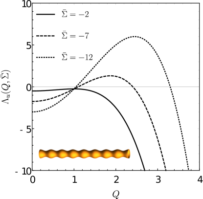
Figure 3: Extensile instability causes a ruffling-like deformation in the shape of the tube. $\Lambda_{u}(Q,\bar{\Sigma})$ is the growth rate of the spatial Fourier modes with time non-dimensionalised by $\tau=\eta r^{2}/\mathcal{K}$ where $\eta$ is the $2$D viscosity, $r$ the tube radius and $\mathcal{K}$ the liquid crystalline splay modulus. The active stress is non-dimensionalised as $\bar{\Sigma}=\Sigma r^{2}/\mathcal{K}$. Inset shows a representative example of such an instability.

In the case of contractile stresses ($\Sigma>0$) we find an instability with fastest growing mode in the $Q\to 0$ limit, Fig. 4 left. This instability is analogous to a classical Rayleigh-Plateau instability (Rayleigh, 1892; Tomotika, 1935) and similar to the pearling instabilities seen in fluid membrane tubes (Gurin et al., 1996; Boedec et al., 2014; Narsimhan et al., 2015). In reality such an instability does not occur at infinite length scales as the dissipative timescale in the ambient media damps the longer wavelength modes. We can approximate the bulk dissipation by modifying our shape dynamics equation in the following manner (Gurin et al., 1996; Boedec et al., 2014; Powers, 2010; Nelson et al., 1995; Al-Izzi et al., 2020b)

$$\Lambda_{u}(Q,\bar{\Sigma})=-\frac{\left(Q^{4}+\left(Q^{2}-1\right)\bar{\Sigma}\right)}{4+8Q^{-2}\tilde{L}_{\text{SD}}^{-1}}\text{,}$$ (74)

where $\tilde{L}_{\text{SD}}=\eta/(\eta_{b}r)$ is the dimensionless Saffman-Delbrück length, and $\eta_{b}$ is the ambient viscosity (Saffman & Delbrück, 1975; Saffman, 1975). Here, this leads to a long wavelength instability as the contractile stress tries to minimise the surface to volume ratio of the tube. This gives a finite wavelength to the fastest growing mode set by the Saffman-Delbrück length, Fig. 4 right. This instability is similar to the isotropic contractile instabilities previously found in fluid membranes (Mietke et al., 2019).

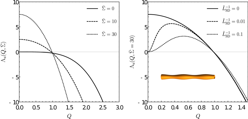
Figure 4: Contractile instability causes a pearling-like deformation in the shape of the tube. $\Lambda_{u}(Q,\bar{\Sigma})$ is the growth rate of the spatial Fourier modes with time non-dimensionalised by $\tau=\eta r^{2}/\mathcal{K}$ where $\eta$ is the $2$D viscosity, $r$ the tube radius and $\mathcal{K}$ the liquid crystalline splay modulus. The active stress is non-dimensionalised as $\bar{\Sigma}=\Sigma r^{2}/\mathcal{K}$. Left: instability in the absence of an ambient fluid. Right: instability when an approximation to ambient hydrodynamics in the long wavelength limit is used. $\tilde{L}_{\text{SD}}=\frac{\eta}{\eta_{b}r}$ is the dimensionless Saffaman-Delbrück length given by ratio of $2$D to $3$D viscosity ($\eta_{b}$) non-dimensionalised by tube radius. Inset shows an example growth of a surface undulation for the case with bulk fluid.

We now turn our attention to the growth rate of the director deviations, which is given by

$$\Lambda_{T}(Q,\bar{\Sigma},\bar{\eta},\nu)=-\frac{\left(\left(Q^{2}+1\right)\left(4\bar{\eta}+(\nu-1)^{2}\right)-2(\nu-1)\bar{\Sigma}\right)}{4}\text{.}$$ (75)

This can also have a change in sign when in both the extensile or contractile regime, depending on the sign of $\nu$ ($\nu<-1$ corresponds to rod-like nematics and $\nu>1$ to disk-like). The stability condition is given by

$$\bar{\Sigma}\geq\frac{(Q^{2}+1)\left(4\bar{\eta}+(\nu-1)^{2}\right)}{2(\nu-1)}\text{,}$$ (76)

which leads to a spontaneous bend instability in the longest wavelengths of the tube, Fig. 5. This instability is well known in flat geometry in the case of extensile stress and rod-like nematics ($\nu<-1$) where it is known to lead to active turbulence (Marchetti et al., 2013).

In the limit $Q\to 0$, this criterion becomes $\bar{\Sigma}\geq\left(4\bar{\eta}+(\nu-1)^{2}\right)/2(\nu-1)$ in comparison to the flat case where the instability is threshold-less Marchetti et al. (2013). This is directly due to the correct use of the surface derivative as the texture needs sufficient active stress to overcome the elastic stress the bend induces by forcing the texture to bend around the tube. Because of this threshold it is interesting to note that the shape instability precedes the bend instability, suggesting it should be possible to generate shape changes before one sees active turbulence. The interplay between this instability and the shape equations beyond linear order is likely a very rich topic as this director instability would likely couple to helical deformation modes leading to a spontaneous chiral symmetry breaking. However such a topic is beyond the scope of the analysis in this paper.

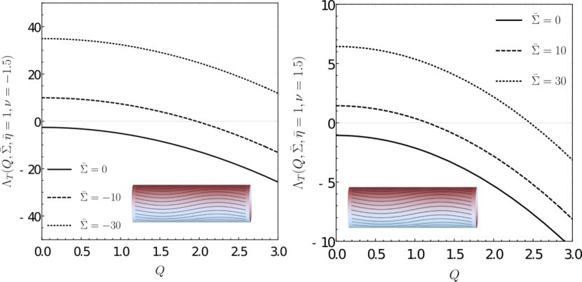
Figure 5: Left: Extensile bend instability in texture on the surface of the tube with rod-like nematics. Right: Contractile bend instability in texture on the surface of the tube with disk-like nematics. $\Lambda_{T}(Q,\bar{\Sigma})$ is the growth rate of the spacial Fourier modes with time non-dimensionalised by $\tau=\eta r^{2}/\mathcal{K}$ where $\eta$ is the $2$D viscosity, $r$ the tube radius and $\mathcal{K}$ the liquid crystalline splay modulus. The active stress is non-dimensionalised as $\bar{\Sigma}=\Sigma r^{2}/\mathcal{K}$. The dimensionless viscosity $\bar{\eta}=1$ and spin connection $\nu=-1.5$ (Left, rod-like nematics) and $\nu=1.5$ (Right, disk-like nematics). Insets shows an example of the bend instability at the longest wavelength of the tube.

3.2.2 Active topological defect deformations

Here we consider a planar membrane in polar Monge coordinates, where the surface is parameterised by the Cartesian vector $\bm{R}=\left(r\cos\theta,r\sin\theta,\epsilon z\right)$. For simplicity we will only consider axisymmetric steady-states, thus $z(r,\theta)=z(r)$. The metric and second fundamental form are given as

$$[g_{\alpha\beta}]=\left(\begin{array}[]{cc}1&0\\ 0&r^{2}\\ \end{array}\right)+O(\epsilon^{2})\text{,}$$ (77)

$$[b_{\alpha\beta}]=\left(\begin{array}[]{cc}\epsilon z_{,rr}&0\\ 0&r\epsilon z_{,\theta}\\ \end{array}\right)+O(\epsilon^{2})\text{,}$$ (78)

up to first order in $\epsilon$. Thus we find $H=\frac{\epsilon}{2}\left(\frac{1}{r}z_{,r}+z_{,rr}\right)+O(\epsilon^{2})$ and $K=0+O(\epsilon^{2})$. We take the polarisation texture to be $\bm{T}=\cos\phi\bm{e}_{r}+\frac{1}{r}\sin\phi\bm{e}_{\theta}$ where $\phi$ is a constant such that there is a $+1$ topological defect located at $r=0$. The continuity equation then yields $v^{r}=0$, so we are left to solve for $z(r,t)$, $\zeta(r,t)$, $\lambda(r,t)$, $v^{\theta}(r,t)$.

At lowest order in $\epsilon$ the the equations are independent of $\dot{z}$ so we look for steady states in the nematic order parameter. Our choice of $\bm{T}$ trivially satisfies the unit magnitude constraint. We now make use of the fact that, at lowest order the tangential force balance and polarization equations are just given by their flat counterparts (that is, they have no $O(\epsilon)$ term) and the shape equation is given entirely by $O(\epsilon)$ terms (Kruse et al., 2005; Hoffmann et al., 2022).

The polarization equations become

$$(\nu\cos(2\phi)-1)\left(v^{\theta}_{,r}-\frac{v^{\theta}}{r}\right)=0\text{,}$$ (79)

$$\nu\sin(\phi)\cos(\phi)\left(v^{\theta}_{,r}-\frac{v^{\theta}}{r}\right)+\lambda+\frac{\mathcal{K}}{\gamma r^{2}}=0\text{,}$$ (80)

which, assuming $\nu>1$ (disk-like nematics), gives

$$\phi=\pm\frac{1}{2}\arccos\left[\frac{1}{\nu}\right]\text{,}$$ (81)

$$\lambda=-\frac{\mathcal{K}}{r^{2}\gamma}-\nu\sin(\phi)\cos(\phi)\left[v^{\theta}_{,r}-\frac{v^{\theta}}{r}\right]\text{.}$$ (82)

Substituting the solution for the $\phi$ into the tangential force balance gives

$$\zeta_{,r}+\frac{\mathcal{K}\nu}{r^{3}}+\frac{\Sigma}{\nu r}=0\text{,}$$ (83)

$$r\left(\eta v^{\theta}_{,r}+\eta rv^{\theta}_{,rr}\pm\sqrt{1-\frac{1}{\nu^{2}}}\Sigma\right)-\eta v^{\theta}=0\text{,}$$ (84)

for which solutions are

$$\zeta=\frac{\mathcal{K}\nu}{2r^{2}}-\frac{\Sigma}{\nu}\log\left[\frac{r}{r_{\text{max}}}\right]+\zeta_{0}\text{,}$$ (85)

$$v^{\theta}=\mp\frac{\Sigma}{2\eta}\sqrt{1-\frac{1}{\nu^{2}}}r\log\left[\frac{r}{r_{\text{max}}}\right]\text{,}$$ (86)

where $\zeta_{0}+\mathcal{K}\nu/2r^{2}_{\text{max}}$ is the surface tension at $r=r_{\text{max}}$. This solution is identical to that found in Kruse et al. (2004) and is one of the classical results of polar active gel theory in a flat geometry. Notice that the surface tension diverges as $r\to 0$ due to the presence of the defect. This divergence in shape can be avoided by introducing a short wavelength cut-off, $r_{c}$, or by considering a more general Landau-de-Gennes free energy that allows for a nematic isotropic phase transition (DeGennes & Prost, 1993).

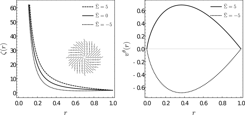
Figure 6: Left: Defect surface tension, $\zeta(r)$, as a function of radius, $r$, about a $+1$ defect centered on $r=0$. Inset is defect texture. Right: Velocity field around the defect. Here we have introduced a small cut-off radius at $r=0.03$ where lengths are non-dimensionalised by the radius of the boundary $r_{\text{max}}=1$. Surface tension is given by $\bar{\zeta}_{0}=\zeta_{0}r_{\text{max}}^{2}/\mathcal{K}=1.0$, spin connection $\nu=1.5$, $r_{c}=0.03$ and $c=-0.05$ where $c$ essentially defines the contact angle at the boundary. The active stress is non-dimensionalised by $\bar{\Sigma}=\sigma r_{\text{max}}/\mathcal{K}$. We plot for both positive (contractile) and negative (extensile) values of active stress to show promotion/suppression of the deformation in each case.

Substituting our solution for the surface tension into the normal force balance equation yields the following dimensionless shape equation

$$\frac{z_{,r}}{r^{3}}\left(7-\nu\left(2\bar{\zeta}_{0}r^{2}+5\right)+2r^{2}\bar{\Sigma}\log(r)+r\left(\sqrt{\nu^{2}-1}+r\bar{\Sigma}\right)\right)$$

$$-\frac{z_{,rr}}{r^{2}}\left(r^{2}(2\bar{\zeta}_{0}\nu+\bar{\Sigma})-2r^{2}\bar{\Sigma}\log(r)+4\right)$$

$$+(\nu+1)\left(z_{,rrrr}+\frac{2}{r}z_{,rrr}\right)=0\text{,}$$ (87)

where lengths have been non-dimensionalised by $r_{\text{max}}$ and energies by $\mathcal{K}$. We can solve this equation numerically with from the boundary ($r=1$ in our dimensionless units) up to a small cut-off, $r_{c}$. We solve with zero mean curvature and derivative in curvature at $r=r_{\text{max}}=1$, at lowest order this is $z^{\prime}(r_{\text{max}})=-z^{\prime\prime}(r_{\text{max}})=z^{\prime\prime\prime}(r_{\text{max}})=c=\text{Const.}$ and fix $z(r_{\text{max}})=0$ at the boundary. The constant, $c$, essentially prescribes the contact angle at the boundary. To solve this numerically we make use of Mathematica (WolframResearch, Champaign, IL).

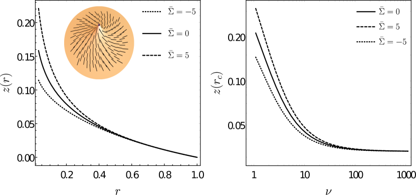
Figure 7: Left: Surface heights, $z(r)$, as a function of radius, $r$, about a $+1$ defect centered on $r=0$. Here we have introduced a small cut-off radius at $r=0.03$ where lengths are non-dimensionalised by the radius of the boundary $r_{\text{max}}=1$. Surface tension is given by $\bar{\zeta}_{0}=\zeta_{0}r_{\text{max}}^{2}/\mathcal{K}=1.0$, spin connection $\nu=1.5$, $r_{c}=0.03$ and $c=-0.05$ where $c$ essentially defines the contact angle at the boundary. The active stress is non-dimensionalised by $\bar{\Sigma}=\sigma r_{\text{max}}/\mathcal{K}$. We plot for both positive (contractile) and negative (extensile) values of active stress to show promotion/suppression of the deformation in each case. Inset is an example surface with the texture shown on top. Right: Maximum defect height, $z(r_{c}=0.03)$, plotted against spin connection $\nu$ (or liquid crystalline Scriven-Love number) in the passive, contractile and extensile cases.

Solutions to this for varying values of active stress are plotted in Fig. 7 with $\bar{\zeta}_{0}=1.0$, $\nu=1.5$, $r_{c}=0.03$ and $c=-0.05$. For $\bar{\Sigma}=0$ we find a convex cusp solution where the stress from the defect causes the surface to buckle. Note that this is qualitatively similar to the full non-linear pseudosphere cusp found in (Frank & Kardar, 2008) although the quantitative details of our shape differ significantly due to our inclusion of the extrinsic curvature term in the Frank free energy, and thus the anisotropic bending energies in our shape equation ($4{{}^{\text{th}}}$ and $3^{\text{rd}}$ order terms) making a full analytical non-linear solution of our equations impossible. For the extensile case, the protrusion decreases in height. The reason for this is directly due to our inclusion of the extrinsic terms in the Frank free energy and the convex shape of the passive solution. Extensile stresses lead to active forces which act to increase bend, in this case bend due to the deformation along the surface, thus pushing the surface down and suppressing the deformation. The opposite is true in the contractile case where the active forces act to flatten bend, thus pushing the surface upward. A simple example of these types effects was discussed in the context of an active fingering instability in Alert (2022). In addition, we show that as the spin connection, $\nu$, (or liquid crystalline Scrinev-Love number) is increased and the spiral defect texture goes from aster-like to vortex-like as $\nu$ goes to $\infty$. As this happens the bend along the surface goes to zero and the height of the defect, $z(r_{c})$, converges in the extensile, contractile and passive cases, as expected.

Note that our results here are different from those seen in Hoffmann et al. (2022) where the effects of contractile and extensile forces are switched. This is straightforward to understand since Hoffmann et al. (2022) did not consider the extrinsic coupling of the director and in addition included an isotropic bending energy. This causes the passive shape to be regularised around the defect and be concave near the defect where the active forces are strongest, leading to a switch in sign of the normal force due to activity when compared to our convex passive shape. Such subtle interplay between passive and active stresses suggests a rich phenomonology of possible non-linear solutions to such systems, and that it may be possible for both extensile and contractile systems to achieve a similar morphology by the varying of passive parameters.

It is interesting to note that the contractile protrusions we find are similar to those seen during Hydra morphogenesis in the underlying contractile actomyosin network (Maroudas-Sacks et al., 2021; Vafa & Mahadevan, 2022). There, the $+1$ defects form the basis of protrusions which develop into “limbs”.

4 Discussion

In this paper we have developed a fully covariant hydrodynamic theory of active nematic fluids on deformable surfaces, deriving equations for normal and tangential force balance along with an equation for order parameter dynamics. Focusing on the case of the one-constant Frank free energy, we identify three dimensionless numbers: two Scriven-Love numbers associated with the ratio of normal viscous forces to bending forces, and an active analogue of the Föppl-von-Kármán number, comparing tangential active stress to bending forces.

We then consider the relaxation dynamics, in shape and order parameter, of a nematic tube with no active forcing, showing that there is a non-trivial coupling between shape and director relaxation in the case of the non-axisymmetric modes. Motivated by the recent interest in active nematic fluids as models of morphogenetic processes, we further consider the effect an active $Q$-tensor term on tube morphology. Here we show that there are several new instabilities in both the contractile and extensile cases, which we compare to similar cases in flat geometry liquid crystals and isotropic fluid membranes. Finally we consider the effect of activity on the surface morphology around a $+1$ topological defect, where anisotropic stresses drive or suppress protrusion of the defect, dependent on whether stresses are contractile or extensile, respectively.

An interesting extension of the problems considered here would be the effect of $1/2$-integer defects on the shape. In addition to breaking axisymmetry, this presents an additional complication in that $+1/2$ integer defects are known to self-propel in active liquid crystals (Giomi et al., 2014). We speculate that such effects would persist (at least in the small deformation limit) and would lead to self-propelled travelling waves in the shape. We aim to explore this phenomenology in detail in future work.

More generally, we believe the framework developed here has applications in a wide range of systems, bridging length and time scales. Our chief interest throughout was to develop the equations in a clear, systematic way that laid bare the basic phenomonology without recourse to biological specifics. With the addition of relevant concentration fields describing morphogens, growth factors and other signalling molecules, these equations could form the basis for a nematic theory of deformable epithelial tissues (Al-Izzi & Morris, 2021; Jülicher et al., 2018). There are also additional areas of potential application in the field of lipid bilayer dynamics; when augmented with isotropic bending energy terms these equations could form the basis for a dynamic theory of tilt-chiral lipid bilayers, extending earlier work considering only energetics (Selinger et al., 1996). It is also plausible that this is the natural framework to model a fluid bilayer coupled to a thin layer of active filaments e.g. actin (Simon et al., 2019), microtubules (Keber et al., 2014) or engineered filaments such as DNA filaments (Jahnke et al., 2022).

A major open challenge in the field of covariant hydrodynamics is developing general stable numerical methods to provide solutions beyond the linear perturbation regime or simple axisymmetric cases (Mietke et al., 2019). A large body of work exists for such problems in the case of passive and active isotropic fluids based on unfitted finite elements, arbitrary Lagrangian-Eulerian finite elements or isogeometric analysis (Barrett et al., 2016; Torres-Sánchez et al., 2019; Vasan et al., 2020; Sahu et al., 2020b), but, to our knowledge, this has yet to be extended to nematic fluids on moving curved surfaces. It is important to note that the equations derived here would likely need to be modified to describe the $Q$-tensor dynamics rather than the nematic order parameter $\bm{T}$ so as to correctly deal with $1/2$ integer defects numerically. Solving such tensor PDEs on curved surfaces is challenging, with issues relating to the discontinuity of basis functions across elements. Although some progress has been made recently in approximating tensor fields numerically using local Monge approximations (Torres-Sánchez et al., 2020).

Current methods for solving nemato-hydrodynamics are often hybrid lattice Boltzmann codes (Denniston et al., 2001; Binysh et al., 2020) and such methods have been used along with phase fields to approximate interface dynamics (Metselaar et al., 2019; Hoffmann et al., 2022). We believe it would also be useful to develop tools to solve the full covariant equations of a deformable mesh using finite element methods so as to provide numerical methods which more clearly map to geometric analytical framework, and thus provide a clearer conceptual link between hydrodynamics and geometry. We therefore welcome further work in this area.

Declaration of interests

The authors report no conflict of interest.

Appendix A Preliminary differential geometry

In this section we define some preliminary objects from differential geometry which we will make use of in the main derivation. We consider a surface, $\mathcal{M}_{t}\subset\mathbb{R}^{3}$ which is locally isomorphic to $\mathbb{R}^{2}$ and changes continuously in time (i.e. the geometry of our interface throughout time is given by a one-parameter family of diffeomorphisms). This assumption neglects any topological changes in the surface and for simplicity we will also consider surfaces without boundary.

We define the embedding of $\mathcal{M}_{t}$ in $\mathbb{R}^{3}$ by the vector $\bm{R}(x_{1},x_{2})$ where we assume that locally one can write this as a function of two parameters $(x_{1},x_{2})$. Within this framework it is possible to define an induced tangent basis on the manifold by taking derivatives with respect to these coordinates $\bm{e}_{\alpha}=\bm{R}_{,\alpha}$ where the subscript, $(,)$, denotes partial differentiation. Note that in general these basis vectors are neither unit, nor orthogonal. From here we can define an induced metric as follows,

$$g_{\alpha\beta}=\bm{R}_{,\alpha}\cdot\bm{R}_{,\beta}=\bm{e}_{\alpha}\cdot\bm{e}_{\beta}$$ (88)

where $g_{\alpha\beta}$ is the metric tensor. It has an inverse, $g^{\alpha\beta}$, defined by $g^{\alpha\beta}g_{\alpha\gamma}=\delta^{\beta}{}_{\gamma}$, it defines an inner product with respect to two vectors in the tangent bundle of $\mathcal{M}_{t}$, and, as such defines a mapping between the tangent bundle and cotangent bundle on $\mathcal{M}_{t}$. This latter point means we can use the metric to map between vectors $\bm{x}=x^{\alpha}\bm{e}_{\alpha}$ and covectors $x=x_{\alpha}\bm{e}^{\alpha}=x^{\beta}g_{\alpha\beta}\bm{e}^{\alpha}$, .i.e. we can use the metric to raise and lower indices.

The metric is sufficient to describe all intrinsic properties of a manifold, however if we also want to know about extrinsic properties, as infact we must if we want to describe how our surface is embedded within $\mathbb{R}^{3}$ then we also require knowledge about how the normal to the surfaces changes. We define a unit normal vector as follows $\bm{\hat{n}}=\bm{e}_{1}\times\bm{e}_{2}/|\bm{e}_{1}\times\bm{e}_{2}|$ where $\times$ is the cross produce in $\mathbb{R}^{3}$. The extrinsic curvature is then defined as the negative of the rate-of-change of the normal in the direction of the tangent basis, and using orthogonality of $\bm{\hat{n}}$ with $\bm{e}_{\alpha}$ we can write

$$b_{\alpha\beta}=\bm{e}_{\alpha,\beta}\cdot\bm{\hat{n}}$$ (89)

where mean and Gaussian curvatures are given by $H=b^{\alpha}{}_{\alpha}/2$ and $K=\mathrm{det}(b^{\alpha}{}_{\beta})$ respectively.

Using orthogonalisty of the normal with the basis vectors and dotting in $\mathbb{R}^{3}$ with $\bm{e}_{\alpha}$ we find the Weingarten relation

$$\bm{\hat{n}}_{,\alpha}=-b^{\beta}{}_{\alpha}\bm{e}_{\beta}$$ (90)

And defining the connection $\Gamma^{\gamma}_{\beta\alpha}=\bm{e}_{\alpha,\beta}\cdot\bm{e}^{\gamma}$ we can find Gauss’s formula

$$\bm{e}_{\alpha,\beta}=\Gamma^{\gamma}_{\alpha\beta}\bm{e}_{\gamma}+b_{\alpha\beta}\bm{\hat{n}}$$ (91)

and we thus define covariant differentiation in the tangent bundle in terms of this connection. The covariant derivative of a rank $(p,q)$ tensor is given by

$$\nabla_{\gamma}T^{\alpha_{1}\dots\alpha_{p}}{}_{\beta_{1}\dots\beta_{q}}= T^{\alpha_{1}\dots\alpha_{p}}{}_{\beta_{1}\dots\beta_{q},\gamma}+\Gamma^{\alpha_{1}}_{\gamma\delta}T^{\delta\dots\alpha_{p}}{}_{\beta_{1}\dots\beta_{q}}+\dots+\Gamma^{\alpha_{p}}_{\gamma\delta}T^{\alpha_{1}\dots\delta}{}_{\beta_{1}\dots\beta_{q}}$$

$$-\Gamma^{\delta}_{\gamma\beta_{1}}T^{\alpha_{1}\dots\alpha_{p}}{}_{\delta\dots\beta_{q}}-\dots-\Gamma^{\delta}_{\gamma\beta_{q}}T^{\alpha_{1}\dots\alpha_{p}}{}_{\beta_{1}\dots\delta}\text{.}$$ (92)

On a torsion free Reimannian manifold the connection is simply given by the Christoffel symbols, which can be written in terms of the metric as

$$\Gamma^{\gamma}_{\alpha\beta}=\frac{1}{2}g^{\gamma\delta}\left(g_{\delta\beta,\alpha}+g_{\delta\alpha,\beta}-g_{\alpha\beta,\delta}\right)\text{.}$$ (93)

A standard measure of intrinsic curvature of a manifold is given by the Reimann tensor, which essentially measures the commutation of two covariant derivatives on a vector (and is thus intimatly related with parallel transport of vectors on surfaces). The Reimann tensor is defined as

$$R^{\tau}{}_{\alpha\gamma\beta}=\Gamma^{\tau}_{\alpha\beta,\gamma}-\Gamma^{\tau}_{\alpha\gamma,\beta}+\Gamma^{\delta}_{\alpha\beta}\Gamma^{\tau}_{\delta\gamma}-\Gamma^{\delta}_{\alpha\gamma}\Gamma^{\tau}_{\delta\beta}\text{.}$$ (94)

For a $d$-dimensional surface equipped with a metric and extrinsic curvature tensor to be embeddable in a $d+1$ dimensional manifold the metric and second fundamental form must satisfy some constraints. These constrains are called the Gauss-Mainardi-Codazzi-Peterson equations, and in the case of a $2$D surface embedded in $\mathbb{R}^{3}$ are given by

$$R^{\tau}{}_{\alpha\beta\gamma}=b^{\tau}{}_{\gamma}b_{\alpha\beta}-b^{\tau}{}_{\beta}b_{\alpha\gamma}$$ (95)

$$b_{\alpha\beta;\gamma}-b_{\alpha\gamma;\beta}=0\text{.}$$ (96)

With some index manipulation one can show that in $2$D the Ricci tensor (a contraction of the Reimann tensor), and Ricci scalar are related to the Gaussian curvature by

$$R_{\alpha\beta}=R^{\gamma}{}_{\alpha\gamma\beta}=Kg_{\alpha\beta}$$ (97)

$$R=R_{\alpha\beta}g^{\alpha\beta}=2K\text{.}$$ (98)

Using this and contracting the Gauss equation (95) gives

$$Kg_{\alpha\beta}=2Hb_{\alpha\beta}-b_{\alpha}{}^{\gamma}b_{\gamma\beta}\text{.}$$ (99)

The manifold $\mathcal{M}_{t}$ is under a flow given by the velocity field $\bm{V}=v^{\alpha}\bm{e}_{\alpha}+v^{(n)}\bm{\hat{n}}\in\mathbb{R}^{3}$. We can calculate the rate-of-change of the basis vectors under this flow as follows

$$\frac{\mathrm{d}}{\mathrm{d}t}\left(\bm{e}_{\alpha}\right) =\bm{V}_{,\alpha}=v^{\beta}{}_{,\alpha}\bm{e}_{\beta}+v^{\beta}\bm{e}_{\beta,\alpha}+v^{(n)}{}_{,\alpha}\bm{\hat{n}}+v^{(n)}\bm{\hat{n}}_{,\alpha}$$

$$=\left(v^{\beta}{}_{;\alpha}-v^{(n)}b^{\beta}{}_{\alpha}\right)\bm{e}_{\beta}+\left(v^{\beta}b_{\alpha\beta}+v^{(n)}{}_{;\alpha}\right)\bm{\hat{n}}$$ (100)

where we have used the Weingarten equation, $\bm{\hat{n}}_{,\alpha}=-b^{\beta}{}_{\alpha}\bm{e}_{\beta}$, and the Gauss formula, $\bm{e}_{\alpha,\beta}=\Gamma^{\gamma}_{\alpha\beta}\bm{e}_{\gamma}+b_{\alpha\beta}\bm{\hat{n}}$. Note that here we have included terms that are advected with the tangential flow, these are important when considering quantities defined in a Lagrangian frame (e.g. the rate-of-deformation tensor), however, when considering objects defined in an objective/Eulerian frame we will only account for changes due to the normal velocity (as in changes that explicitly change the surface geometry). There are more concise ways to write these derivatives in a mixed Lagrangian-Eulerian manner, but this makes use of Lie derivatives so we avoid this here for the sake of simplicity.

We now proceed to calculate the time derivative of the normal vector, $\bm{\hat{n}}$, the first point to note is that $\frac{\mathrm{d}}{\mathrm{d}t}(|\bm{\hat{n}}|^{2})=0\Rightarrow\bm{\hat{n}}\cdot\frac{\mathrm{d}}{\mathrm{d}t}(\bm{\hat{n}})=0$ i.e. there are no normal components. Next using the fact that $\bm{e}_{\alpha}\cdot\bm{\hat{n}}=0$ (by construction), we find the following

$$\frac{\mathrm{d}}{\mathrm{d}t}\left(\bm{\hat{n}}\right)=-\bm{V}_{,\alpha}\cdot\bm{\hat{n}}g^{\alpha\beta}\bm{e}_{\beta}=-\left(v^{\beta}b_{\beta}{}^{\alpha}+v^{(n)}{}_{;\alpha}g^{\alpha\beta}\right)\bm{e}_{\alpha}\text{.}$$ (101)

In deriving the exact form of each of the functional derivatives the following geometric identities will prove useful. Throughout this paper we will make use of rate equations for geometric quantities in order to compute functional derivatives as we believe this simplifies computations somewhat as we will only be computing first variations in the energy.

Starting from the definition of the second fundamental form, (89), we have

$$\frac{\mathrm{d}}{\mathrm{d}t}\left(b_{\alpha\beta}\right)=\left(\frac{\mathrm{d}}{\mathrm{d}t}\bm{e}_{\alpha,\beta}\right)\cdot\bm{\hat{n}}+\bm{e}_{\alpha,\beta}\cdot\frac{\mathrm{d}}{\mathrm{d}t}\bm{\hat{n}}\text{.}$$ (102)

Examining the first term we find

$$\frac{\mathrm{d}}{\mathrm{d}t}\bm{e}_{\alpha,\beta}\cdot\bm{\hat{n}}=\bm{V}_{,\alpha\beta}\cdot\bm{\hat{n}}$$ (103)

where

$$\bm{V}_{,\alpha\beta} =\Big{[}\left(v^{\gamma}{}_{;\alpha}-v^{(n)}b^{\gamma}{}_{\alpha}\right)\bm{e}_{\gamma}+\left(v^{\gamma}b_{\alpha\gamma}+v^{(n)}{}_{,\alpha}\right)\bm{\hat{n}}\Big{]}_{,\beta}$$

$$=\left(v^{\gamma}{}_{;\alpha}-v^{(n)}b^{\gamma}{}_{\alpha}\right)_{,\beta}\bm{e}_{\gamma}+\left(v^{\gamma}{}_{;\alpha}-v^{(n)}b^{\gamma}{}_{\alpha}\right)\bm{e}_{\gamma,\beta}$$

$$+\left(b_{\alpha\gamma}v^{\gamma}\right)_{,\beta}\bm{\hat{n}}+v^{(n)}{}_{,\alpha\beta}\bm{\hat{n}}+\left(v^{\gamma}b_{\alpha\gamma}+v^{(n)}{}_{,\alpha}\right)\bm{\hat{n}}_{,\beta}$$ (104)

Dotting with $\bm{\hat{n}}$ and making use of the Gauss’s formula and Weingarten equation (91) & (90) we find

$$\bm{V}_{,\alpha\beta}\cdot\bm{\hat{n}}=\left(v^{\gamma}{}_{;\alpha}-v^{(n)}b^{\gamma}{}_{\alpha}\right)b_{\gamma\beta}+\left(b_{\alpha\gamma}v^{\gamma}\right)_{,\beta}+v^{(n)}{}_{,\alpha\beta}\text{.}$$ (105)

Making use of the equation for the normal vector dynamics, (101), dotting with $\bm{e}_{\alpha,\beta}$, and making use of the Gauss’s formula we find

$$\bm{e}_{\alpha,\beta}\cdot\frac{\mathrm{d}}{\mathrm{d}t}\bm{\hat{n}}=-\Gamma^{\gamma}_{\alpha\beta}v^{\delta}b_{\gamma\delta}-\Gamma^{\gamma}_{\alpha\beta}v^{(n)}_{,\gamma}\text{.}$$ (106)

The equation for the time derivative of $b_{\alpha\beta}$ then becomes

$$\frac{\mathrm{d}}{\mathrm{d}t}b_{\alpha\beta}=\left(v^{\gamma}{}_{;\alpha}-v^{(n)}b^{\gamma}{}_{\alpha}\right)b_{\gamma\beta}+\left(b_{\alpha\gamma}v^{\gamma}\right)_{;\beta}+v^{(n)}_{;\alpha\beta}\text{.}$$ (107)

Finally we make use of (99) to give $b_{\alpha}{}^{\gamma}b_{\gamma\beta}=2Hb_{\alpha\beta}-Kg_{\alpha\beta}$ and the symmetry under exchange of indices of $b_{\alpha\beta}$ and the Codazzi equation (96) to rewrite $b_{\alpha\gamma;\beta}v^{\gamma}=v^{\gamma}b_{\alpha\beta;\gamma}$ and we find

$$\frac{\mathrm{d}}{\mathrm{d}t}b_{\alpha\beta}=v^{\gamma}b_{\alpha\beta;\gamma}+b_{\alpha\gamma}v^{\gamma}{}_{;\beta}+b_{\gamma\beta}v^{\gamma}{}_{;\alpha}+v^{(n)}_{,\alpha;\beta}-v^{(n)}\left(2Hb_{\alpha\beta}-Kg_{\alpha\beta}\right)\text{.}$$ (108)

The rate of the area element is given by (Frankel, 2011; Arroyo & DeSimone, 2009)

$$\dot{\mathrm{d}A}=-2Hv^{(n)}\mathrm{d}A\text{.}$$ (109)

Finally the rate-of-change of the Christoffel symbols is given by (Frankel, 2011)

$$\frac{\mathrm{d}}{\mathrm{d}t}\Gamma^{\gamma}_{\alpha\beta}=\frac{1}{2}g^{\gamma\delta}\left(\left(\frac{\mathrm{d}}{\mathrm{d}t}g_{\alpha\delta}\right)_{;\beta}+\left(\frac{\mathrm{d}}{\mathrm{d}t}g_{\beta\delta}\right)_{;\alpha}-\left(\frac{\mathrm{d}}{\mathrm{d}t}g_{\alpha\beta}\right)_{;\delta}\right)\text{.}$$ (110)

References

- Al-Izzi & Morris (2021) Al-Izzi, S. C. & Morris, R. G. 2021 Active flows and deformable surfaces in development. Seminars in Cell and Developmental Biology 120, 44–52.
- Al-Izzi et al. (2020a) Al-Izzi, S. C., Sens, P. & Turner, M. S. 2020a Shear-driven instabilities of membrane tubes and dynamin-induced scission. Phys. Rev. Lett. 125, 018101.
- Al-Izzi et al. (2020b) Al-Izzi, S. C., Sens, P., Turner, M. S. & Komura, S. 2020b Dynamics of passive and active membrane tubes. Soft Matter 16, 9319.
- Alert (2022) Alert, R. 2022 Fingering instability in active nematic droplets. J. Phys. A: Math. Theor. 55, 234009.
- Arroyo & DeSimone (2009) Arroyo, M. & DeSimone, A. 2009 Relaxation dynamics of fluid membranes. Phys. Rev. E 79, 031915.
- Audoly & Pomeau (2010) Audoly, B. & Pomeau, Y. 2010 Elasticity and Geometry: From Hair Curls to the Non-linear Response of Shells. OUP Oxford.
- Bächer et al. (2021) Bächer, C., Khoromskaia, D., Salbreux, G. & Gekle, S. 2021 A three-dimensional numerical model of an active cell cortex in the viscous limit. Front. Phys. 9, 753230.
- Barrett et al. (2016) Barrett, J. W., Garcke, H. & Nürnberg, R. 2016 A stable numerical method for the dynamics of fluidic membranes. Numerische Mathematik 134, 783–822.
- Bell et al. (2022) Bell, S., Lin, S.-Z., Rupprecht, J.-F. & Prost, J. 2022 Active nematic flows over curved surfaces. Phys. Rev. Lett. 129, 118001.
- Binysh et al. (2020) Binysh, J., Z̆. Kos, C̆opar, S., Ravnik, M. & Alexander, G. P. 2020 Three-dimensional active defect loops. Phys. Rev. Lett. 124, 088001.
- Blanch-Mercader et al. (2021a) Blanch-Mercader, C., Guillamat, P., Roux, A. & Kruse, K. 2021a Integer topological defects of cell monolayers: Mechanics and flows. Phys. Rev. E 103, 012405.
- Blanch-Mercader et al. (2021b) Blanch-Mercader, C., Guillamat, P., Roux, A. & Kruse, K. 2021b Quantifying material properties of cell monolayers by analyzing integer topological defects. Phys. Rev. Lett. 126, 028101.
- Boedec et al. (2014) Boedec, G., Jaeger, M. & Leonetti, M. 2014 Pearling instability of a cylindrical vesicle. J. Fluid Mech. 743, 262–279.
- DeGennes & Prost (1993) DeGennes, P. G. & Prost, J. 1993 The Physics of Liquid Crystals. Clarendon Press.
- Denniston et al. (2001) Denniston, C., Orlandini, E. & Yeomans, J. M. 2001 Lattice boltzmann simulations of liquid crystal hydrodynamics. Phys. Rev. E 63, 056702.
- Doi (2011) Doi, M. 2011 Onsager’s variational principle in soft matter. J. Phys.: Condens. Matter 23, 284118.
- Doostmohammadi et al. (2018) Doostmohammadi, A., Ignés-Mullol, J., Yeomans, J. M. & Sagués, F. 2018 Active nematics. Nature Communications 9, 3246.
- Edwards & Yeomans (2009) Edwards, S. A. & Yeomans, J. M. 2009 Spontaneous flow states in active nematics: A unified picture. EPL 85, 18008.
- Fernández-Nieves et al. (2007) Fernández-Nieves, A., Link, D. R., Márquez, M. & Weitz, D. A. 2007 Topological changes in bipolar nematic droplets under flow. Phys. Rev. Lett. 98, 087801.
- Fournier & Galatola (2007) Fournier, J.-B. & Galatola, P. 2007 Critical fluctuations of tense fluid membrane tubules. Phys. Rev. Lett. 98, 018103.
- Frank (1958) Frank, F. C. 1958 I. liquid crystals. on the theory of liquid crystals. Discussions of the Faraday Society 25, 19–28.
- Frank & Kardar (2008) Frank, J. R. & Kardar, M. 2008 Defects in nematic membranes can buckle into pseudospheres. Phys. Rev. E 77, 041705.
- Frankel (2011) Frankel, T. 2011 The Geometry of Physics: An Introduction. Cambridge University Press.
- Giomi et al. (2014) Giomi, L., Bowick, M. J., Mishra, P., Sknepnek, R. & Marchetti, M. C. 2014 Defect dynamics in active nematics. Philosophical Transactions of the Royal Society A: Mathematical, Physical and Engineering Sciences 372, 20130365.
- Gurin et al. (1996) Gurin, K. L., Lebedev, V. V. & Muratov, A. R. 1996 Dynamic instability of a membrane tube. JETP 83, 321–326.
- Hoffmann et al. (2022) Hoffmann, L. A., Carenza, L. N., Eckert, J. & Giomi, L. 2022 Defect-mediated morphogenesis. Science Advances 8, eabk2712.
- Hu et al. (2007) Hu, D., Zhang, P. & E, Weinan 2007 Continuum theory of a moving membrane. Phys. Rev. E 75, 041605.
- Jahnke et al. (2022) Jahnke, K., Huth, V., Mersdorf, U., Liu, N. & Göpfrich, K. 2022 Bottom-up assembly of synthetic cells with a dna cytoskeleton. ACS Nano 16, 7233–7241.
- Jülicher et al. (2018) Jülicher, F., Grill, S. W. & Salbreux, G. 2018 Hydrodynamic theory of active matter. Rep. Prog. Phys. 81, 076601.
- Keber et al. (2014) Keber, F. C., Loiseau, E., Sanchez, T., DeCamp, S. J., Giomi, L., Bowick, M. J., Marchetti, M. C., Dogic, Z. & Bausch, A. R. 2014 Topology and dynamics of active nematic vesicles. Science 645, 1135–1139.
- Khoromskaia & Alexander (2017) Khoromskaia, D. & Alexander, G. P. 2017 Vortex formation and dynamics of defects in active nematic shells. New Journal of Physics 19, 103043.
- Khoromskaia & Salbreux (2021) Khoromskaia, D. & Salbreux, G. 2021 Active morphogenesis of patterned epithelial shells. arXiv:2111.12820 .
- Kruse et al. (2004) Kruse, K., Joanny, J.-F., Jülicher, F., Prost, J. & Sekimoto, K. 2004 Asters, vortices, and rotating spirals in active gels of polar filaments. Phys. Rev. Lett. 92, 078101.
- Kruse et al. (2005) Kruse, K., Joanny, J.-F., Jülicher, F., Prost, J. & Sekimoto, K. 2005 Generic theory of active polar gels: a paradigm for cytoskeletal dynamics. Eur. Phys. J. E 16, 5–16.
- Lee (1997) Lee, John M. 1997 Riemannian manifolds: an introduction to curvature. Graduate texts in mathematics 176. Springer.
- Marchetti et al. (2013) Marchetti, M. C., Joanny, J.-F., Ramaswamy, S., Liverpool, T. B., Prost, J., Rao, M. & Simha, R. A. 2013 Hydrodynamics of soft active matter. Rev. Mod. Phys. 85, 1143–1189.
- Maroudas-Sacks et al. (2021) Maroudas-Sacks, Y., Garion, L., Shani-Zerbib, L., Livshits, A., Braun, E. & Kinneret, K. 2021 Topological defects in the nematic order of actin fibres as organization centres of hydra morphogenesis. Nature Physics 17, 251–259.
- Marsden & Hughes (1994) Marsden, J. E. & Hughes, T. J. R. 1994 Mathematical Foundations of Elasticity. Dover Publications.
- Metselaar et al. (2019) Metselaar, L., Yeomans, J. M. & Doostmohammadi, A. 2019 Topology and morphology of self-deforming active shells. Phys. Rev. Lett. 123, 208001.
- Mietke et al. (2019) Mietke, A., Jülicher, F. & Sbalzarini, I. F. 2019 Self-organized shape dynamics of active surfaces. Proc. Nat. Acc. Sci. 116, 29–34.
- Naganathan et al. (2014) Naganathan, S. R., Fürthauer, S., Nishikawa, M., Jülicher, F. & Grill, S. W. 2014 Active torque generation by the actomyosin cell cortex drives left–right symmetry breaking. eLife 3, e04165.
- Napoli & Vergori (2012) Napoli, G. & Vergori, L. 2012 Extrinsic curvature effects on nematic shells. Phys. Rev. Lett. 108, 207803.
- Napoli & Vergori (2016) Napoli, G. & Vergori, L. 2016 Hydrodynamic theory for nematic shells: The interplay among curvature, flow, and alignment. Phys. Rev. E 94, 020701(R).
- Narsimhan et al. (2015) Narsimhan, V., Spann, A. P. & Shaqfeh, E. S. G. 2015 Pearling, wrinkling, and buckling of vesicles in elongational flows. J. Fluid Mech. 777, 1–26.
- Needham (2021) Needham, T. 2021 Visual Differential Geometry and Forms: A Mathematical Drama in Five Acts. Princeton University Press.
- Nelson et al. (1995) Nelson, P., Powers, T. & Seifert, U. 1995 Dynamical theory of the pearling instability in cylindrical vesicles. Phys. Rev. Lett. 74, (17)3384.
- Nestler & Voigt (2022) Nestler, M. & Voigt, A. 2022 Active nematodynamics on curved surfaces – the influence of geometric forces on motion patterns of topological defects. Commun. Comput. Phys. 31, 947–965.
- Nitschke & Voigt (2022) Nitschke, I. & Voigt, A. 2022 Observer-invariant time derivatives on moving surfaces. Journal of Geometry and Physics 173, 104428.
- Pearce (2020) Pearce, D. J. G. 2020 Defect order in active nematics on a curved surface. New Journal of Physics 22, 063051.
- Pearce et al. (2019) Pearce, D. J. G., Ellis, P. W., Fernandez-Nieves, A. & Giomi, L. 2019 Geometrical control of active turbulence in curved topographies. Phys. Rev. Lett. 122, 168002.
- Powers (2010) Powers, T. 2010 Dynamics of filaments and membranes in a viscous fluid. Rev. Mod. Phys. 82, 1607–1631.
- Prost et al. (2015) Prost, J., Jülicher, F. & Joanny, J.-F. 2015 Active gel physics. Nature Physics 11, 111–117.
- Ramaswamy (2017) Ramaswamy, S. 2017 Active matter. Journal of Statistical Mechanics: Theory and Experiment p. 054002.
- Rangamani et al. (2013) Rangamani, P., Agrawal, A., Mandadapu, K. K., Oster, G. & Steigmann, D. J. 2013 Interaction between surface shape and intra-surface viscous flow on lipid membranes. Biomech Model Mechanobiol 12, 833.
- Rank & Voigt (2021) Rank, M. & Voigt, A. 2021 Active flows on curved surfaces. Physics of Fluids 33, 072110.
- Rayleigh (1892) Rayleigh, Lord 1892 On the instability of a cylinder of viscous liquid under capillary force. The London, Edinburgh, and Dublin Philosophical Magazine and Journal of Science 34, 145–154.
- da Rocha et al. (2022) da Rocha, H. B., Bleyer, J. & Turlier, H. 2022 A viscous active shell theory of the cell cortex. J. Mech. Phys. Solids 164, 104876.
- Saffman (1975) Saffman, P. G. 1975 Brownian motion in thin sheets of viscous fluid. J. Fluid Mech. 73, 593–602.
- Saffman & Delbrück (1975) Saffman, P. G. & Delbrück, M. 1975 Brownian motion in biological membranes. Proc. Nat. Acc. Sci. 72, 3111–3113.
- Sahu et al. (2020a) Sahu, A., Glisman, A., Tchoufag, J. & Mandadapu, K. K. 2020a Geometry and dynamics of lipid membranes: The scriven-love number. Phys. Rev. E 101, 052401.
- Sahu et al. (2020b) Sahu, A., Omar, Y. A. D., Sauer, R. A. & Mandadapu, K. K. 2020b Arbitrary lagrangian–eulerian finite element method for curved and deforming surfaces i. general theory and application to fluid interfaces. J. Comp. Phys. 407, 109253.
- Salbreux & Jülicher (2017) Salbreux, G. & Jülicher, F. 2017 Mechanics of active surfaces. Phys. Rev. E 96, 032404.
- Salbreux et al. (2022) Salbreux, G., Jülicher, F., Prost, J. & Callen-Jones, A. 2022 Theory of nematic and polar active fluid surfaces. Phys. Rev. Res. 4, 033158.
- Sanchez et al. (2012) Sanchez, T., Chen, D. T. N., DeCamp, S. J., Heymann, M. & Dogic, Z. 2012 Spontaneous motion in hierarchically assembled active matter. Nature 491, 431–435.
- Santiago (2018) Santiago, J. A. 2018 Stresses in curved nematic membranes. Phys. Rev. E 97, 052706.
- Santiago et al. (2019) Santiago, J. A., Chacón-Acosta, G. & Monroy, F. 2019 Membrane stress and torque induced by frank’s nematic textures: A geometric perspective using surface-based constraints. Phys. Rev. E 100, 012704.
- Santiago & Monroy (2020) Santiago, J. A. & Monroy, F. 2020 Mechanics of nematic membranes: Euler–lagrange equations, noether charges, stress, torque and boundary conditions of the surface frank’s nematic field. J. Phys. A: Math. Theor. 53, 165201.
- Saw et al. (2017) Saw, T. B., Doostmohammadi, A., Nier, V., Kocgozlu, L., Thampi, S., Toyama, Y., Marcq, P., Lim, C. T., Yeomans, J. M. & Ladoux, B. 2017 Topological defects in epithelia govern cell death and extrusion. Nature 544, 212–216.
- Scriven (1960) Scriven, L. E. 1960 Dynamics of a fluid interface equation of motion for newtonian surface fluids. Chemical Engineering Science 12, 98–108.
- Selinger et al. (1996) Selinger, J. V., MacKintosh, F. C. & Schnur, J. M. 1996 Theory of cylindrical tnbilles and helical ribbons of chiral lipid membranes. Phys. Rev. E 53, 043804.
- Simon et al. (2019) Simon, C., Kusters, R., Caorsi, V., Allard, A., Abou-Ghali, M., Manzi, J., Cicco, A. Di, Lévy, D., Lenz, M., Joanny, J.-F., Campillo, C., Plastino, J., Sens, P. & Sykes, C. 2019 Actin dynamics drive cell-like membrane deformation. Nature Physics 15, 602–609.
- Steigmann (1999) Steigmann, D. J. 1999 Fluid films with curvature elasticity. Arch. Rational Mech. Anal. 150, 127.
- Tchoufag et al. (2022) Tchoufag, J., Sahu, A. & Mandadapu, K. K. 2022 Absolute vs convective instabilities and front propagation in lipid membrane tubes. Phys. Rev. Lett. 128, 068101.
- Terzi & Deserno (2017) Terzi, M. M. & Deserno, M. 2017 Novel tilt-curvature coupling in lipid membranes. J. Chem. Phys. 147, 084702.
- Tomotika (1935) Tomotika, S. 1935 On the instability of a cylindrical thread of a viscous liquid surrounded by another viscous fluid. Proceedings of the Royal Society of London. Series A - Mathematical and Physical Sciences 150, 322–337.
- Torres-Sánchez et al. (2019) Torres-Sánchez, A., Millán, D. & Arroyo, M. 2019 Modelling fluid deformable surfaces with an emphasis on biological interfaces. J. Fluid Mech. 872, 218–271.
- Torres-Sánchez et al. (2020) Torres-Sánchez, A., Santos-Oliván, D. & Arroyo, M. 2020 Approximation of tensor fields on surfaces of arbitrary topology based on local monge parametrizations. J. Comp. Phys. 405, 109168.
- Vafa & Mahadevan (2022) Vafa, F. & Mahadevan, L. 2022 Active nematic defects and epithelial morphogenesis. Phys. Rev. Lett. 129, 098102.
- Vasan et al. (2020) Vasan, R., Rudraraju, S., Akamatsu, M., Garikipati, K. & Rangamani, P. 2020 A mechanical model reveals that non-axisymmetric buckling lowers the energy barrier associated with membrane neck constriction. Soft Matter 16, 784.
- Waxman (1984) Waxman, A. M. 1984 Dynamics of a couple-stress fluid membrane. Studies in Applied Mathematics 70, 63–86.
- Zhong-Can & Helfrich (1989) Zhong-Can, O.-Y. & Helfrich, W. 1989 Bending energy of vesicle membranes: General expressions for the first, second, and third variation of the shape energy and applications to spheres and cylinders. Phys. Rev. A 39, 5280.