Struct-MDC: Mesh-Refined Unsupervised Depth Completion Leveraging Structural Regularities from Visual SLAM

Abstract

Feature-based visual simultaneous localization and mapping (SLAM) methods only estimate the depth of extracted features, generating a sparse depth map. To solve this sparsity problem, depth completion tasks that estimate a dense depth from a sparse depth have gained significant importance in robotic applications like exploration. Existing methodologies that use sparse depth from visual SLAM mainly employ point features. However, point features have limitations in preserving structural regularities owing to texture-less environments and sparsity problems. To deal with these issues, we perform depth completion with visual SLAM using line features, which can better contain structural regularities than point features. The proposed methodology creates a convex hull region by performing constrained Delaunay triangulation with depth interpolation using line features. However, the generated depth includes low-frequency information and is discontinuous at the convex hull boundary. Therefore, we propose a mesh depth refinement (MDR) module to address this problem. The MDR module effectively transfers the high-frequency details of an input image to the interpolated depth and plays a vital role in bridging the conventional and deep learning-based approaches. The Struct-MDC outperforms other state-of-the-art algorithms on public and our custom datasets, and even outperforms supervised methodologies for some metrics. In addition, the effectiveness of the proposed MDR module is verified by a rigorous ablation study.

I Introduction

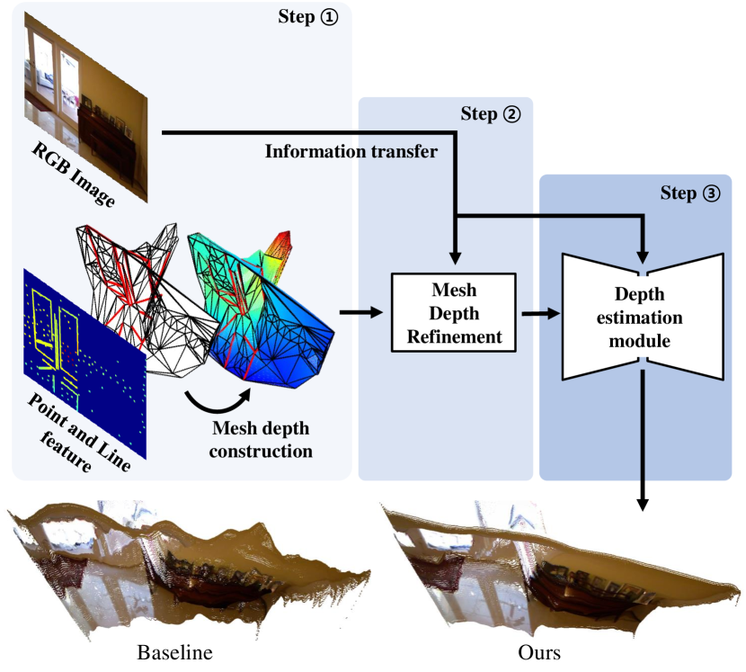
Figure 1: The proposed three-step method for depth completion. KBNet [1] is employed as a baseline in the third step. Our method effectively captures object boundary using line features, which are colored in red, from visual SLAM.

Feature-based visual simultaneous localization and mapping (SLAM) methods use only partial information of an image, and are efficient for computationally complex cases. Therefore, compared with direct methods, which use complete pixel information of an image, indirect methods can be commonly used on devices with limited computing power [2], and many studies have been conducted on them [3, 4]. However, there is no method for determining the depth information of the remaining pixels that are not extracted as features by the indirect methods. In addition, the maximum number of used features is limited to tens to hundreds per input image frame to reduce the computation, thereby causing sparsity of the depth data. Therefore, the sparse depth maps generated by indirect methods provide insufficient topology or structural information of the surroundings of a robot. These shortcomings make it difficult for indirect methods to be used directly for exploration and path planning, which are essential applications of SLAM.

To deal with the map sparsity problem of indirect methods, depth completion tasks are being actively studied. Depth completion usually estimates a dense depth using a sparse depth information from visual SLAM with deep learning. Different from mono-depth prediction [5], which suffers from scale ambiguity, the absolute scale from the sparse feature depth facilitates depth completion close to the ground truth. However, most existing depth completion methods rely only on implicit learning of their models to estimate a dense depth. As pointed out in [6], if all the inference results solely rely on deep learning, a model may fall into a local minimum to fill empty spaces with only copy and paste to minimize the loss. Therefore, countermeasures are needed to resolve these problems.

Recent studies on depth completion from visual SLAM have mainly focused on the generation of dense depth from point feature depth. However, in a methodology that utilizes the point features, it is difficult to capture the complete structural regularities of the environment. In addition, point features have the disadvantage of being susceptible to dynamic illumination and texture-less environments. In terms of SLAM, studies on using line features as new measurements are being actively conducted [7, 8, 9] to overcome the shortcomings of point features. As in the case of state estimation, line features provide powerful spatial information in depth completion tasks and complement the shortcomings of deep learning-based approaches, in which depth estimation at the boundary of an object becomes ambiguous. However, attempts to apply this new measurement to depth completion have not yet been actively conducted. Therefore, to resolve the problems of existing methods caused by point features, in this study, line features are utilized for depth completion. To this end, we propose the methodology shown in Fig. 1, which utilizes most of the advantages of line features, instead of simply passing point and line features as model inputs.

The main contributions of this study are as follows:

• To the best of our knowledge, the Struct-MDC (mesh-refined unsupervised depth completion leveraging structural regularities from visual SLAM) is the first to introduce line features from line-based SLAM into a depth completion task.

• To utilize line features efficiently, unlike other existing deep learning-based methodologies that rely on implicit learning, we propose a mesh depth refinement (MDR) module with an explicit three-step approach: structural sketch, refinement, and estimation with constrained Delaunay triangulation (CDT) [10] using line features.

• To prove the validity of Struct-MDC, the state-of-the-art performance for depth completion tasks is verified by experiments on public datasets and our custom dataset. The code and dataset of the proposed algorithm are publicly available at: https://github.com/zinuok/line_depth_completion.

The remainder of this paper is organized as follows: Section II reviews related studies. Section III describes the proposed method in detail and Section IV presents a detailed analysis of the experimental results. Finally, Section V summarizes our contributions as well as future works.

II Related Works

II-A Supervised Depth Completion

In a supervised method, the model learns to directly minimize the error between a ground truth depth and its estimation. The RGB and sparse depth images have different modalities. To fuse the heterogeneous modality inputs, early fusion [11], late fusion [12], and multi-stage fusion [13] methods have been proposed. Using uncertainty estimation, Teixeira et al. [14] effectively dealt with depth completion on an aerial platform involving diverse depth and viewpoints. Sartipi et al. [15] utilized surface normal prediction and plane detection for depth enrichment of sparse inputs, focusing on a planar structure that is frequently observed in indoor environments. Matsuki et al. [16] combined prediction from a variational autoencoder network with conventional multiple view optimization. Supervised methods facilitate easy learning, with excellent performance. However, there is a limitation in that accurately acquiring numerous ground truth depth in the real world is difficult, promoting the need for unsupervised learning.

II-B Unsupervised Depth Completion

In unsupervised depth estimation frameworks, the photometric discrepancy between actual and reconstructed images using a multiple view geometry has been used as a supervisory signal [17, 18]. This scheme is also applicable to unsupervised depth completion frameworks [19, 20]. Owing to the lack of ground truth depth, several techniques are used to assist model learning in unsupervised methodologies. Among them, classical techniques may help a model understand the scene topology. In [21], a lightweight network using Delaunay triangulation was presented. However, its accuracy is limited because the triangulation generated by point features does not fit well in the case of complex structures. Wong et al. [1] utilized the camera’s intrinsic parameter as an input to improve the generalization performance of a model by feature encoding back-projection into 3D space. However, this method still depends on a front-end pooling layer to densify sparse point depth. In [22], a topology prior learned from a synthetic dataset was refined on the real-world dataset. However, max pooling used to fill the empty depth misses the detailed depth information of an object. The aforementioned methods still have problems resulting from point features. To overcome this issue, there is a need to introduce a new type of measurement.

II-C Edge Awareness and Depth Refinement

Edges play vital roles in depth estimation because they can identify the depth discontinuity at an object boundary. Motivated by [23], Jiang et al. [24] adopted a random point selection scheme to utilize pervasive line and plane structures in an indoor environment as supervisory signals. In [25], the Manhattan world assumption and vanishing point clustering were employed to estimate surface normals with increased accuracy. Ferstl et al. [26] investigated the use of the super-resolution methodology of depth images by the edge-aware energy optimization. Edge awareness can also support a depth refinement task [27], which refines coarse depth estimated by a model guided by an image. Khamsis et al. [28] added detailed information to a disparity map estimated from stereo images by dilating or eroding around the edges with iterative hierarchical refinement. Qi et al. [29] refined initial surface normal and depth estimations by generating a weight map with edges extracted from an image. Because depth completion inherits the essential properties of depth estimation, it can benefit from edge awareness. However, attempts to introduce the edge awareness advantage from line feature depth into a depth completion framework have not been actively conducted.

III Struct-MDC

III-A Overall Framework

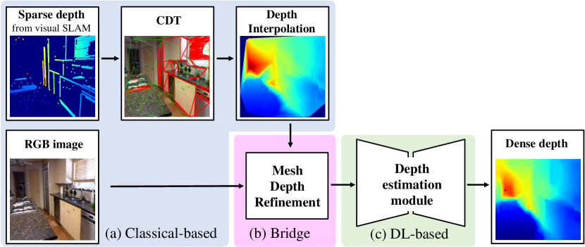
Figure 2: Overall network architecture of struct-MDC: dense depth is estimated through (a) structural sketch and interpolation, (b) refinement, and (c) estimation.

Our objective is to estimate a pixel-wise depth, given an RGB image and a sparse feature depth from visual SLAM. The overall framework of struct-MDC is shown in Fig. 2. The proposed method is explicitly split into three steps: structural sketch, refinement, and estimation. In the structural sketch step, struct-MDC uses point and line features extracted from visual SLAM. Using these features, a mesh with structural regularities is generated by CDT. Using the constructed mesh, a rough mesh depth is generated by depth interpolation. Owing to discontinuities and low-frequency detail problems, the generated mesh depth is unsuitable for direct use as an input to the main module. Therefore, an MDR module is proposed. The MDR module acts as a bridge to generate a refined mesh depth and transfer detailed information from the given RGB image to the rough mesh depth. At last, the final dense depth is estimated by the main module. As a baseline, the main encoder-decoder architecture of [1] is adopted. Its front-end sparse-to-dense module is excluded because our structural sketch and interpolation followed by refinement can effectively replace the module. We assume that the surrounding environment structure is piecewise planar and rectilinear for the framework proposed in this study. The struct-MDC is expressed as follows:

$$\begin{gathered}\mathbf{z}_{d}=f\circ g\circ h(I,\mathcal{P},\mathcal{L},\mathbf{K}),\\ \mathcal{P}:=\bigcup^{m}_{i=1}(\mathbf{x}_{p_{i}},z_{p_{i}}),\\ \mathcal{L}:=\bigcup^{n}_{j=1}(l_{j}(\mathbf{x}_{s_{j}};\mathbf{x}_{e_{j}}),z_{s_{j}},z_{e_{j}}),\end{gathered}$$ (1)

where $\mathbf{z}_{d}$ denotes the densified depth; $f$, $g$, and $h$ denote functions of the depth estimation, refinement, and structural sketch steps; $I$ and $\mathbf{K}$ denote the RGB image and the camera’s intrinsic parameter; $\mathcal{P}$ and $\mathcal{L}$ denote sets of point and line features with depth; $\mathbf{x}_{p_{i}}$, $\mathbf{x}_{s_{j}}$, and $\mathbf{x}_{e_{j}}$ represent the $i$-th 2D point feature, the start and end points of the $j$-th 2D line feature $l_{j}$; and $m$ and $n$ are the numbers of point and line features; $z_{p_{i}}$, $z_{s_{j}}$, and $z_{e_{j}}$ denote the depth of the $i$-th point feature, those of the start and end points of the $j$-th line feature, respectively.

III-B Structural Sketch by Constrained Delaunay Triangulation

In this stage, a rough mesh depth is generated from a sparse feature depth based on the classical methodology. Construction of the rough mesh depth requires mesh generation using features. As shown in Figs. 3 and 4, line features are formed at the object boundary, supporting our rectilinear assumption. Line features better represent the structural regularities of an environment than point features. Therefore, we use CDT to create a mesh using point and line features. Different from [21], in which triangulation was performed with only point features, CDT can strongly leverage the structural regularities of a human-made environment, because the detected line features are included as constrained edges, as shown in Figs. 33 and 3. Owing to this advantage, CDT is performed using point and line features as follows:

$$\begin{gathered}(\mathcal{F},\mathcal{V},\mathcal{E})=\mathcal{C}\left(\bigcup^{m}_{i=1}\mathbf{x}_{p_{i}},\bigcup^{n}_{j=1}l_{j}(\mathbf{x}_{s_{j}};\mathbf{x}_{e_{j}})\right),\end{gathered}$$ (2)

where $\mathcal{C}$ denotes a CDT generation function that uses point and line features as input; $\mathcal{F}$, $\mathcal{V}$, and $\mathcal{E}$ denote triangle facets, vertices, and edges of CDT, respectively. Using CDT, a line feature is explicitly included in the $\mathcal{E}$ as constrained edges.

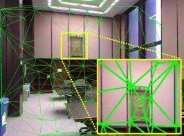
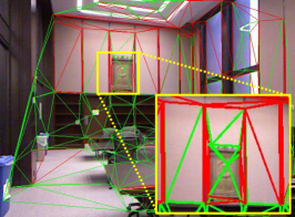
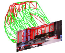
Figure 3: Constructed meshes with 3 only point features and 3 point and line features (ours). 3 Back-projected mesh into 3D space. The line features are colored in red.

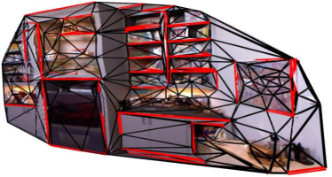
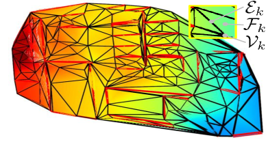
Figure 4: Before 4 and after 4 mesh depth interpolation. The line features are colored in red.

Using the depth information of the point and line features included in the $\mathcal{V}$ and $\mathcal{E}$, the 2D mesh on the image is back-projected into a 3D space, as shown in Fig. 33. The 3D mesh contains the depth information only at the vertices and edges corresponding to the point and line features. Therefore, to fill the depth of triangle facet using the boundary depth information, linear interpolation is performed, as shown in Fig. 4, and it is expressed as follows:

$$\begin{gathered}\mathbf{z}_{m}=h(\mathcal{F},\mathcal{V},\mathcal{E},\mathcal{P},\mathcal{L}),\end{gathered}$$ (3)

where $h$ denotes back-projection into a 3D space followed by linear depth interpolation; $\mathbf{z}_{m}$ represents the rough mesh depth.

III-C Mesh Depth Refinement Module

There are two major problems with the generated mesh depth: depth discontinuity and low-frequency depth. The point and line feature sets are bounded inside the image plane. At this time, because the mesh constructed by CDT forms a convex hull, its area cannot exceed the entire image area. Therefore, a depth outside the convex hull cannot be interpolated, producing a depth discontinuity at its boundary. The area padded with zeros adversely affects the neuron activation of the network. Another major problem is that a simple linear interpolation will eliminate high-frequency information in the interpolated depth. Therefore, details of the actual object are lost. To solve these problems, the MDR module shown in Fig. 5 is proposed.

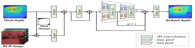
Figure 5: Proposed mesh depth refinement (MDR) module. Introducing mask channel and parallel pooling facilitates the module to learn the discontinuity and complementary spatial information, respectively.

Motivated by [27], the MDR module performs refinement by transferring high-frequency detail from an RGB image to low-frequency discontinuous mesh depth as follows:

$$\mathbf{z}_{r}=g(I,\mathbf{z}_{m}),$$ (4)

where $\mathbf{z}_{r}$ denotes the refined mesh depth. Specifically, to deal with the depth discontinuity problem, the binary mask channel extracted from the mesh depth is concatenated in the form of hypercolumns. The mask channel transmits information about the discontinuity in advance, enabling the first convolution of the RGB image branch to adaptively transfer information depending on the presence of depth. The concatenated channel also helps deliver information outside the convex hull. Subsequently, similar to the original module which uses max pooling, multiscale feature fusion is performed to learn the spatial information. In particular, parallel pooling is proposed for downsampling. Existing methodologies with only max pooling defect detailed information because only the strong activation signals from color and depth images are extracted. To compensate this deficiency, min and max pooling are fused complementarily as parallel branches.

III-D Depth Estimation

For estimating the dense depth, the calibrated back-projection network proposed in [1] is adopted as a main module. Their sparse-to-dense module is excluded because the proposed structural sketch and refinement steps effectively replace the front-end module. Taking the refined mesh depth as the input, the main module estimates a dense depth as follows:

$$\mathbf{z}_{d}=f(I,\mathbf{z}_{r},\mathbf{K}),$$ (5)

where $\mathbf{z}_{d}$ denotes the estimated dense depth. In the calibrated back-projection layer, the model uses a camera’s intrinsic parameter as input. After the encoded feature map from the RGB image is back-projected with the encoded depth and the camera’s intrinsic parameter, 3D positional encoding is performed.

III-E Loss Function

The loss commonly employed for unsupervised depth completion is used for the regression of the proposed network. Please note that the proposed MDR module can be integrated into the entire system without any additional loss function. Therefore, some notations used in the baseline [1] are adopted in this study. The overall loss is calculated as follows:

$$L=w_{p}l_{p}+w_{s}l_{s}+w_{l}l_{l},$$ (6)

where $l_{p}$, $l_{s}$, and $l_{l}$ denote the photometric consistency, sparse depth consistency, and local smoothness loss; $w_{p}$, $w_{s}$, and $w_{l}$ denote their corresponding weights, respectively.

III-E1 Photometric consistency loss

Using the estimated depth and the relative pose between consecutive frames, the photometric error between the reconstructed and actual images can be defined as follows:

$$l_{p}=\frac{1}{|\Omega|}\sum_{t^{\prime}\in{\rm T}}\sum_{p\in\Omega}w_{1}\|I(\mathbf{x})-I_{t^{\prime}\rightarrow t}(\mathbf{x})\|$$ (7)

$$+w_{2}(1-{SSIM}(I(\mathbf{x})-I_{t^{\prime}\rightarrow t}(\mathbf{x}))),$$

where ${\rm T}$ denotes a time sequence; $I_{t^{\prime}\rightarrow t}$ and $I_{t}$ denote the warped image from $t^{\prime}$ to $t$ and the actual image at $t$; $\mathbf{x}$ and $\Omega$ represent a single pixel and the collection of all pixels of the image; and $w_{1}$ and $w_{2}$ denote the corresponding photometric discrepancy weights, respectively. $SSIM$ is the structural similarity index defined in [30] as follows:

$$SSIM(\alpha,\beta)=\frac{(2\mu_{\alpha}\mu_{\beta}+C_{1})(2\sigma_{\alpha\beta}+C_{2})}{(\mu^{2}_{\alpha}+\mu^{2}_{\beta}+C_{1})(\sigma^{2}_{\alpha}+\sigma^{2}_{\beta}+C_{2})},$$ (8)

where $\alpha$ and $\beta$ denote images to compare; $\mu$ and $\sigma$ denote the mean intensity and the standard deviation; $C_{1}$ and $C_{2}$ represent small constants for mathematical stability, respectively.

III-E2 Sparse depth consistency loss

For a provided feature depth, the regression can be conducted using the information obtained by measuring the residual between the prediction from the network and the feature depth as follows:

$$l_{s}=\frac{1}{|\Omega_{v}|}\sum_{\mathbf{x}\in\Omega_{v}}{(\|\mathbf{z}_{d}(\mathbf{x})-\mathbf{z}_{f}(\mathbf{x})\|)},$$ (9)

where $\mathbf{z}_{f}$ and $\Omega_{v}$ denote the point and line feature depth and a set of valid pixels with a sparse depth, respectively.

III-E3 Local smoothness loss

To ensure the smoothness of the depth of a particular object, the gradient of the estimated depth is used as follows:

$$l_{l}=\frac{1}{|\Omega|}\sum_{\mathbf{x}\in\Omega}{e^{-|\partial_{x}I(\mathbf{x})|}|\partial_{x}\mathbf{z}_{d}(\mathbf{x})|+e^{-|\partial_{y}I(\mathbf{x})|}|\partial_{y}\mathbf{z}_{d}(\mathbf{x})|}.$$ (10)

A pixel area with a large image gradient is penalized to accommodate the depth discontinuity at the object boundary.

IV Experimental Results

This section is organized as follows: The effectiveness of our proposed framework is verified in Section IV.C. An ablation study is conducted for the proposed MDR module in Section IV.D.

IV-A Implementation Details

Our network is trained on a single NVIDIA TITAN V GPU with 12 GB memory. The batch size is set as 4 for the VOID [21], and NYUv2 [31] datasets, and 2 for our custom point-line feature and depth (PLAD) dataset considering the memory capacity. For training, the Adam optimizer with exponential decay rates of $\beta_{1}=0.9$ and $\beta_{2}=0.999$ is used. The learning rate initialized as $1\times 10^{-4}$ decays by half at 20 epochs, and is set as $5\times 10^{-5}$ up to 30 epochs. In addition, the loss weights are set as $w_{p}=1.0$, $w_{s}=0.6$, $w_{l}=0.04$, $w_{1}=0.15$, and $w_{2}=0.95$. After image undistortion for line extraction and cropping, $608\times 448$ size images are used for the VOID and NYUv2 datasets, and $1280\times 720$ size images are used for the PLAD dataset.

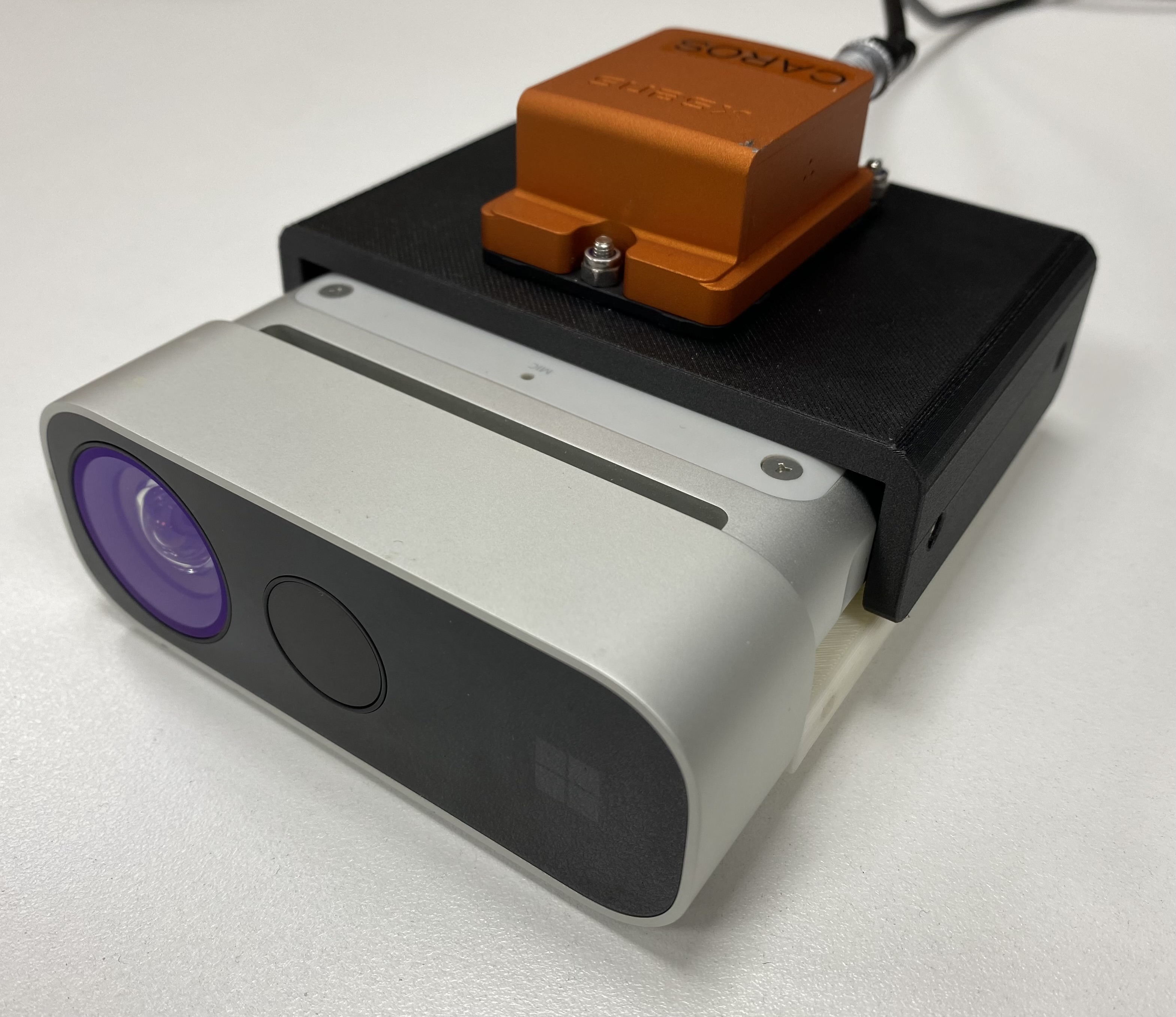
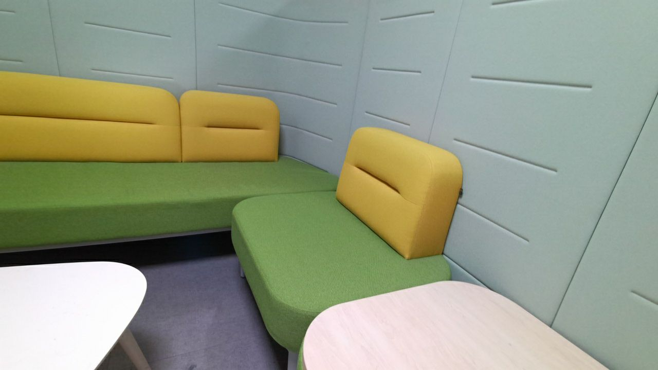
Figure 6: Our PLAD dataset: 6 Sensor setup consists of RGB-D camera and IMU. Sequences acquired 6 indoor and 6 outdoor

IV-B Datasets

IV-B1 VOID

This dataset provides synchronized RGB images ($640\times 480$), ground truth depth images ($640\times 480$), inertial measurement unit (IMU) data from Intel D435i, and sparse point features from visual-inertial odometry [32]. Because Struct-MDC additionally utilizes line features, UV-SLAM [33] is executed to detect point and line features and generate sparse depth. However, owing to the challenges with substantial motion blur of the provided sequences, the ground truth depth is sampled using the feature matching results of the SLAM front-end. Of the total 56 sequences, 47 sequences are used for training, 8 for testing, and 1 with poor feature detection and mesh results is excluded.

IV-B2 NYUv2

This dataset provides synchronized RGB images ($640\times 480$) and ground truth depth images ($640\times 480$) from Microsoft Kinect. Because this dataset does not provide the IMU data required to execute UV-SLAM, the ground truth depth is sampled as in the VOID dataset. Post-processed data with filled depth values are used as in [11]. According to the official split, 48K frames are used for training and 654 frames for testing.

IV-B3 PLAD

A sparse depth is inevitably sampled from the ground truth depth in the aforementioned datasets, which are far from the genuine depth completion from visual SLAM. Therefore, we generate a PLAD dataset where sparse depth is provided by line-based visual SLAM to verify Struct-MDC. As shown in Fig. 66, the data are acquired with a sensor setup consisting of an Azure Kinect for ground truth depth with RGB images ($1280\times 720$, 15 Hz) and an Xsens Mti-100 for IMU data (6-axis, 200 Hz). The depth and RGB images are synchronized with the feature depth estimated using UV-SLAM. Each sequence is acquired in various environments, as shown in Figs. 66 and 6. The PLAD dataset consists of 38 sequences, with 34 sequences used for training and 4 sequences for testing. More detailed information such as the sensor calibration data is available at: https://github.com/zinuok/line_depth_completion.

IV-C Results of Analysis

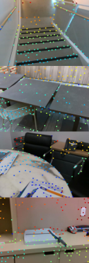
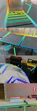
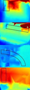
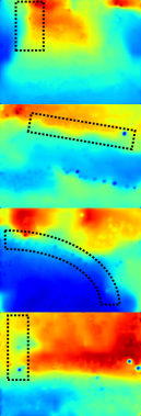
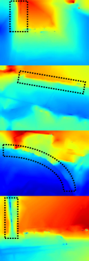
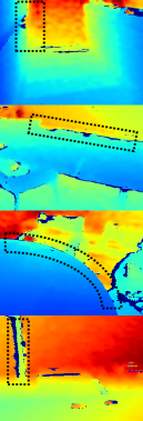
Figure 7: Qualitative comparison results for the VOID: 7 The extracted point features, 7 the extracted point and line features from UV-SLAM [33]. Completed depth from 7 [21], 7 [1], and 7 Struct-MDC. 7 Ground truth depth. The dashed rectangles denote the area where the improvement in the Struct-MDC stands out.

Table I: Quantitative comparison with state-of-the-arts methods for the VOID dataset. (pre: results using their pretrained weights. re: results using retrained weights.)

Method		Error [mm] $\downarrow$		Accuracy [%] $\uparrow$
		MAE	RMSE	$\delta_{1}$	$\delta_{2}$	$\delta_{3}$
VOICED [21]	(pre)	167.608	316.017	57.499	74.014	96.974
	(re)	163.530	283.763	32.327	74.762	98.559
FusionNet [22]	(pre)	167.600	346.533	55.455	72.721	97.866
	(re)	166.143	337.522	58.841	73.894	96.346
KBNet (baseline) [1]	(re)	143.801	262.643	52.286	69.494	98.724
Struct-MDC (ours)		111.332	216.497	62.074	74.544	99.003

Error metrics commonly adopted for the performance evaluation of depth estimation tasks [1, 34] are as follows: mean absolute error (MAE), root mean squared error (RMSE), and accuracy ratio under a threshold $\delta$ which is an absolute ratio between the estimation and the ground truth depth. In our experiments, overall statistical analysis is based on the MAE and RMSE, and strict thresholds $\delta_{1}=1.05$, $\delta_{2}=1.10$, and $\delta_{3}=1.25^{3}$ are used to measure the extent of closeness to the ground truth.

Struct-MDC used a new type of measurement: a line feature. Therefore, depending on the dataset, the effect of line measurements is verified in various scenarios. In the VOID and the NYUv2 datasets, the total number of point and line features is limited to 150. In the PLAD dataset, the point and line features estimated from the UV-SLAM are used without constraints on the total number.

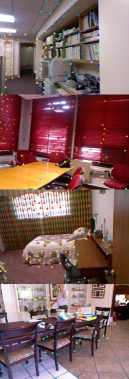
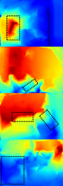
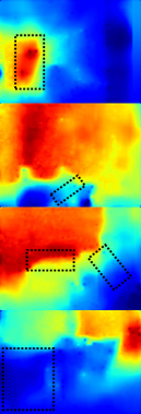
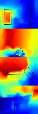
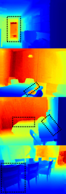
Figure 8: Qualitative comparison results for the NYUv2: 8 The extracted point features, 8 the extracted point and line features from UV-SLAM [33]. Completed depth from 8 [21], 8 [1], and 8 Struct-MDC. 8 Ground truth depth. The dashed rectangles denote the area where the improvement in the Struct-MDC stands out.

Table II: Quantitative comparison with state-of-the-arts methods for the NYUv2 dataset. (pre: results using their pretrained weights. re: results using retrained weights. U: unsupervised, S: supervised )

Method			Error [mm] $\downarrow$			Accuracy [%] $\uparrow$
			MAE	RMSE		$\delta_{1}$	$\delta_{2}$	$\delta_{3}$
VOICED [21]	U	(pre)	244.416	407.979		54.488	71.107	97.255
		(re)	205.898	328.202		56.965	74.747	99.401
FusionNet [22]	U	(pre)	223.111	353.720		51.878	69.801	99.282
		(re)	208.399	360.653		57.162	74.335	98.879
KBNet (baseline) [1]	U	(re)	179.817	297.872		59.605	78.027	99.346
Struct-MDC (ours)	U		141.871	245.548		67.991	81.999	99.698
CSPN [35]	S	(re)	163.152	245.864		59.092	84.656	99.861

IV-C1 Comparison for the VOID dataset

In a human-made environment, many line features are observed at the object boundary, as shown in Fig. 77. The method proposed in [21] depends only on the depth from triangulation of point feature. Therefore, as shown in Fig. 77, the method frequently generated incorrect triangles, estimating an ambiguous depth with mesh facet imprints. Our baseline, KBNet [1], has stains in several scenarios, as shown in Fig. 77. It can be seen that traces of copy and paste remain in the final estimation because they rely on the pooling layer to fill the low density of point features. In contrast, Struct-MDC does not contain any stains or incorrect imprints. Ours employs the interpolation and MDR sequentially to fill the empty space. Therefore, the roles of the two modules are adequately separated, eliminating the stains and improving the overall performance. An object boundary, which was disregarded in other methods, exists as a line feature and an edge of a triangle in the proposed algorithm. Consequently, such boundaries are more apparent in the final result, making the distinction between objects noticeable. Remarkably, a curved boundary such as a circular table can also be estimated based on our piecewise linear assumption. The performance improvement can be quantitatively seen from TABLE I. In Struct-MDC, the MAE and the RMSE are improved by $22.58\%$ and $17.57\%$, compared with the state-of-the-art [1], respectively.

IV-C2 Comparison for the NYUv2 dataset

The qualitative comparison results are shown in Fig. 8. As in the experiments for the VOID dataset, traces of triangulation remain in [21] and stains are observed in [1]. However, our methodology estimates a depth close to the ground truth with the support of line features. In particular, Struct-MDC excels in regions where point features are not extracted, as shown in the first row or for structural objects as shown in the fourth row of Fig. 8. The performance improvement can be seen from the results in TABLE II. The MAE and RMSE of Struct-MDC are improved by $21.10\%$ and $17.57\%$, respectively, compared to those of the state-of-the-art method [1]. The average processing time of Struct-MDC was increased to 32.19 ms (31.07 Hz), compared to that of the baseline, 15.46 ms (64.68 Hz). However, it is still fast enough to be exploited to real robot applications. It is noteworthy that Struct-MDC outperforms the supervised method, CSPN [35], in terms of all error metrics and the accuracy metric of $\delta_{1}$, even though ours is an unsupervised method.

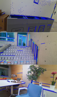
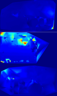
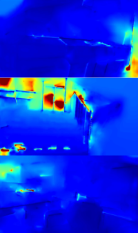
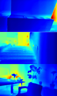
Figure 9: Qualitative comparison results for the PLAD: 9 point and line features from UV-SLAM [33], 9 interpolated mesh, 9 completed depth from Struct-MDC, and 9 ground truth depth.

Table III: Quantitative comparison with state-of-the-arts methods for the PLAD dataset.

Method	Error [mm] $\downarrow$		Accuracy [%] $\uparrow$
	MAE	RMSE	$\delta_{1}$	$\delta_{2}$	$\delta_{3}$
KBNet (baseline) [1]	5512.334	5595.194	$\simeq$ 0.000	$\simeq$ 0.000	9.183
Struct-MDC (ours)	1170.303	1481.583	4.567	8.899	67.071

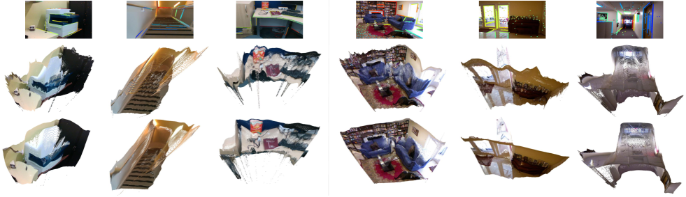
Figure 10: 3D visualization of estimated depth for the VOID (left three columns) and NYUv2 (right three columns) datasets: Detected features (top row), estimated depth from our baseline (middle row), and proposed method (bottom row). The proposed method noticeably aligns object boundary with reduced jittering.

IV-C3 Comparison for the PLAD dataset

In this dataset, the spatial distribution of the features is non-uniform, and there is considerable uncertainty in the estimated depth from visual SLAM. As can be inferred from TABLE III, the baseline presents deficient performance and fails to converge. However, Struct-MDC can successfully estimate the entire depth because the empty area is significantly reduced by the generation of a convex hull using point and line features, as shown in Fig. 99.

The main reason for the failure of the baseline is that there is no method to effectively deal with the no-feature area outside the convex hull. The baseline requires the assumption that at least one sparse feature is included in the kernel size of the pooling layer for densification. This assumption is reasonably applied inside the convex hull where sparse features exist, whereas it is ineffective if the proportion of the no-feature areas becomes larger than the overall size of the image. Actually, the estimated point features in the PLAD dataset are extremely sparse, $0.02\%$, compared to those in the previous two datasets, $0.05\%$. Struct-MDC also partially loses its accuracy. Nevertheless, Struct-MDC is robust to the distribution and density condition. This is because Struct-MDC additionally utilizes the line features which compensate the sparsity of point features from visual SLAM. In addition, the depth can be estimated even outside the convex hull without depth information by using the MDR module.

IV-C4 3D visualization results

For a straightforward comparison, Fig. 10 shows the 3D depth images estimated by the baseline and Struct-MDC on the VOID and NYUv2 datasets. The results of the baseline show an inaccurate jittering at the object boundary, which is significantly reduced by Struct-MDC. Struct-MDC can also more accurately estimate the depth inside the object than the baseline, by accurately capturing the object boundary.

IV-D Ablation Study: Mesh Depth Refinement module

An ablation study was performed on two datasets to rigorously demonstrate the effectiveness of the proposed MDR module. If line features are employed, the model performance is expected to be improved as the given prior increases. Nonetheless, simply using a line feature as a model input cannot fully exploit the potential of the line. Fig. 11 and TABLE IV show error plots and quantitative results according to input, respectively. P, L, M, and R denote point input, line input, mesh input, and refined mesh input, respectively. The overall error is decreased when the mesh is employed compared to that when simply using point and line features. The error was significantly reduced when the mesh refinement was performed. When line features are simply used as an additional input to the network, blur holes still exist at the object boundary. The holes imply that the local smoothness loss, $l_{l}$, intensely reflects the penalty for accommodating the depth discontinuity in the object boundary, and that the network fell into a local minimum with a simple copy and paste. Because the baseline employs a pooling layer for densification, and the model is prone to fall into this local minimum. In contrast, blur holes are removed with the interpolated mesh depth as the input, whereas the object boundary is captured sufficiently. This is because the empty depth is filled by interpolation with awareness of the object boundary by CDT. The advantage of using a mesh emerges if the proposed MDR module is utilized jointly. Compared to the case where point and line features are simply used in the baseline model (P + L), the proposed methodology (P + L + M + R) dramatically improves the overall performance.

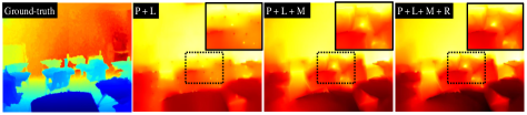
Figure 11: Error plots of different input methods with ground truth depth. In three error figures on right, bright color implies large error.

Table IV: Ablation study: Effectiveness of proposed mesh depth refinement module. (P: point feature, L: line feature, M: interpolated mesh, R: proposed refinement module. )

Dataset	Method	Error [mm] $\downarrow$		Accuracy [%] $\uparrow$
		MAE	RMSE	$\delta_{1}$	$\delta_{2}$	$\delta_{3}$
VOID	P (baseline)	143.801	262.643	52.286	69.494	98.724
	P + L	124.243	235.622	58.642	72.745	98.949
	P + L + M	120.917	228.467	58.741	73.418	99.002
	P + L + M + R	111.332	216.497	62.074	74.544	99.003
NYUv2	P (baseline)	179.817	297.872	59.605	78.027	99.346
	P + L	163.618	270.276	62.230	79.185	99.500
	P + L + M	144.853	248.293	67.381	81.728	99.687
	P + L + M + R	141.871	245.548	67.991	81.999	99.698

V Conclusions

In summary, this study introduced line features from visual SLAM as new measurements to a depth completion task for the first time. For this, a three-step approach to efficiently use line features: structural sketch, refinement, and estimation, was proposed with a bridge module between the conventional and deep learning approaches. Struct-MDC was proven to achieve state-of-the-art performance based on experiments with various datasets. Furthermore, an ablation study proved that the CDT mesh with the MDR module significantly increases the overall performance. Line features have strong potential in that it captures the depth discontinuity at the object boundary, which is a continuing deep learning problem. Nevertheless, depth completion utilizing line features from visual SLAM is an area that has not been actively explored. Therefore, to contribute to this society, we disclose our code and the custom dataset, PLAD. The limitation of Struct-MDC is that the average processing time was slightly increased compared to the baseline. We will optimize the model for future works to reduce the processing time and apply it to real robot exploration.

References

- [1] A. Wong and S. Soatto, “Unsupervised depth completion with calibrated backprojection layers,” in Proc. IEEE/CVF International Conference on Computer Vision (ICCV), 2021, pp. 12 747–12 756.
- [2] J. Jeon, S. Jung, E. Lee, D. Choi, and H. Myung, “Run your visual-inertial odometry on NVIDIA Jetson: Benchmark tests on a micro aerial vehicle,” IEEE Robotics and Automation Letters, vol. 6, no. 3, pp. 5332–5339, 2021.
- [3] T. Qin, P. Li, and S. Shen, “VINS-Mono: A robust and versatile monocular visual-inertial state estimator,” IEEE Transactions on Robotics, vol. 34, no. 4, pp. 1004–1020, 2018.
- [4] A. Rosinol, M. Abate, Y. Chang, and L. Carlone, “Kimera: an open-source library for real-time metric-semantic localization and mapping,” in Proc. IEEE International Conference on Robotics and Automation (ICRA), 2020, pp. 1689–1696. [Online]. Available: https://github.com/MIT-SPARK/Kimera
- [5] T. Zhou, M. Brown, N. Snavely, and D. G. Lowe, “Unsupervised learning of depth and ego-motion from video,” in Proc. IEEE Conference on Computer Vision and Pattern Recognition (CVPR), 2017, pp. 1851–1858.
- [6] Y.-K. Huang, T.-H. Wu, Y.-C. Liu, and W. H. Hsu, “Indoor depth completion with boundary consistency and self-attention,” in Proc. IEEE/CVF International Conference on Computer Vision (ICCV) Workshops, 2019, pp. 1070–1078.
- [7] R. Gomez-Ojeda, J. Briales, and J. Gonzalez-Jimenez, “PL-SVO: Semi-direct monocular visual odometry by combining points and line segments,” in Proc. IEEE/RSJ International Conference on Intelligent Robots and Systems (IROS), 2016, pp. 4211–4216.
- [8] J. Lee and S.-Y. Park, “PLF-VINS: Real-time monocular visual-inertial SLAM with point-line fusion and parallel-line fusion,” IEEE Robotics and Automation Letters, vol. 6, no. 4, pp. 7033–7040, 2021.
- [9] H. Lim, Y. Kim, K. Jung, S. Hu, and H. Myung, “Avoiding degeneracy for monocular visual SLAM with point and line features,” in Proc. IEEE International Conference on Robotics and Automation (ICRA), 2021, pp. 11 675–11 681.
- [10] L. P. Chew, “Constrained Delaunay triangulations,” Algorithmica, vol. 4, no. 1, pp. 97–108, 1989.
- [11] F. Ma and S. Karaman, “Sparse-to-dense: Depth prediction from sparse depth samples and a single image,” in Proc. IEEE International Conference on robotics and automation (ICRA), 2018, pp. 4796–4803.
- [12] C. Fu, C. Dong, C. Mertz, and J. M. Dolan, “Depth completion via inductive fusion of planar LiDAR and monocular camera,” in Proc. IEEE/RSJ International Conference on Intelligent Robots and Systems (IROS), 2020, pp. 10 843–10 848.
- [13] Z. Huang, J. Fan, S. Cheng, S. Yi, X. Wang, and H. Li, “HMS-Net: Hierarchical multi-scale sparsity-invariant network for sparse depth completion,” IEEE Transactions on Image Processing, vol. 29, pp. 3429–3441, 2019.
- [14] L. Teixeira, M. R. Oswald, M. Pollefeys, and M. Chli, “Aerial single-view depth completion with image-guided uncertainty estimation,” IEEE Robotics and Automation Letters, vol. 5, no. 2, pp. 1055–1062, 2020.
- [15] K. Sartipi, T. Do, T. Ke, K. Vuong, and S. I. Roumeliotis, “Deep depth estimation from Visual-Inertial SLAM,” in Proc. IEEE/RSJ International Conference on Intelligent Robots and Systems (IROS), 2020, pp. 10 038–10 045.
- [16] H. Matsuki, R. Scona, J. Czarnowski, and A. J. Davison, “CodeMapping: Real-time dense mapping for sparse SLAM using compact scene representations,” IEEE Robotics and Automation Letters, vol. 6, no. 4, pp. 7105–7112, 2021.
- [17] H. Zhan, R. Garg, C. S. Weerasekera, K. Li, H. Agarwal, and I. Reid, “Unsupervised learning of monocular depth estimation and visual odometry with deep feature reconstruction,” in Proc. IEEE Conference on Computer Vision and Pattern Recognition (CVPR), 2018, pp. 340–349.
- [18] Y. Almalioglu, M. R. U. Saputra, P. P. de Gusmao, A. Markham, and N. Trigoni, “GANVO: Unsupervised deep monocular visual odometry and depth estimation with generative adversarial networks,” in Proc. IEEE International Conference on robotics and automation (ICRA), 2019, pp. 5474–5480.
- [19] F. Ma, G. V. Cavalheiro, and S. Karaman, “Self-supervised sparse-to-dense: Self-supervised depth completion from LiDAR and monocular camera,” in Proc. IEEE International Conference on Robotics and Automation (ICRA), 2019, pp. 3288–3295.
- [20] J. Choi, D. Jung, Y. Lee, D. Kim, D. Manocha, and D. Lee, “SelfDeco: Self-supervised monocular depth completion in challenging indoor environments,” in Proc. IEEE International Conference on Robotics and Automation (ICRA), 2021, pp. 467–474.
- [21] A. Wong, X. Fei, S. Tsuei, and S. Soatto, “Unsupervised depth completion from visual inertial odometry,” IEEE Robotics and Automation Letters, vol. 5, no. 2, pp. 1899–1906, 2020.
- [22] A. Wong, S. Cicek, and S. Soatto, “Learning topology from synthetic data for unsupervised depth completion,” IEEE Robotics and Automation Letters, vol. 6, no. 2, pp. 1495–1502, 2021.
- [23] M. A. Fischler and R. C. Bolles, “Random sample consensus: a paradigm for model fitting with applications to image analysis and automated cartography,” Communications of the ACM, vol. 24, no. 6, pp. 381–395, 1981.
- [24] H. Jiang, L. Ding, J. Hu, and R. Huang, “PLNet: Plane and line priors for unsupervised indoor depth estimation,” in Proc. International Conference on 3D Vision (3DV), 2021, pp. 741–750.
- [25] R. Wang, D. Geraghty, K. Matzen, R. Szeliski, and J.-M. Frahm, “VPLNet: Deep single view normal estimation with vanishing points and lines,” in Proc. IEEE/CVF International Conference on Computer Vision and Pattern Recognition (CVPR), 2020, pp. 689–698.
- [26] D. Ferstl, C. Reinbacher, R. Ranftl, M. Rüther, and H. Bischof, “Image guided depth upsampling using anisotropic total generalized variation,” in Proc. IEEE International Conference on Computer Vision (ICCV), 2013, pp. 993–1000.
- [27] S. Yan, C. Wu, L. Wang, F. Xu, L. An, K. Guo, and Y. Liu, “DDRNet: Depth map denoising and refinement for consumer depth cameras using cascaded cnns,” in Proc. European Conference on Computer Vision (ECCV), 2018, pp. 151–167.
- [28] S. Khamis, S. Fanello, C. Rhemann, A. Kowdle, J. Valentin, and S. Izadi, “StereoNet: Guided hierarchical refinement for real-time edge-aware depth prediction,” in Proc. European Conference on Computer Vision (ECCV), 2018, pp. 573–590.
- [29] X. Qi, Z. Liu, R. Liao, P. H. S. Torr, R. Urtasun, and J. Jia, “GeoNet++: Iterative geometric neural network with edge-aware refinement for joint depth and surface normal estimation,” IEEE Transactions on Pattern Analysis and Machine Intelligence, vol. 44, no. 2, pp. 969–984, 2022.
- [30] Z. Wang, A. C. Bovik, H. R. Sheikh, and E. P. Simoncelli, “Image quality assessment: from error visibility to structural similarity,” IEEE Transactions on Image Processing, vol. 13, no. 4, pp. 600–612, 2004.
- [31] N. Silberman, D. Hoiem, P. Kohli, and R. Fergus, “Indoor segmentation and support inference from RGBD images,” in Proc. European Conference on Computer Vision (ECCV), 2012, pp. 746–760.
- [32] X. Fei, A. Wong, and S. Soatto, “Geo-supervised visual depth prediction,” IEEE Robotics and Automation Letters, vol. 4, no. 2, pp. 1661–1668, 2019.
- [33] H. Lim, J. Jeon, and H. Myung, “UV-SLAM: Unconstrained line-based SLAM using vanishing points for structural mapping,” IEEE Robotics and Automation Letters, vol. 7, no. 2, pp. 1518–1525, 2022.
- [34] C. Cadena, Y. Latif, and I. D. Reid, “Measuring the performance of single image depth estimation methods,” in Proc. IEEE/RSJ International Conference on Intelligent Robots and Systems (IROS), 2016, pp. 4150–4157.
- [35] X. Cheng, P. Wang, and R. Yang, “Depth estimation via affinity learned with convolutional spatial propagation network,” in Proc. European Conference on Computer Vision (ECCV), 2018, pp. 103–119.