22email: {spraman3,carlosdc,rchella4}@jhu.edu,
ewa.m.nowara@gmail.com,gleason@umd.edu
Where in the World is this Image?
Transformer-based Geo-localization in the Wild
Abstract
Predicting the geographic location (geo-localization) from a single ground-level RGB image taken anywhere in the world is a very challenging problem. The challenges include huge diversity of images due to different environmental scenarios, drastic variation in the appearance of the same location depending on the time of the day, weather, season, and more importantly, the prediction is made from a single image possibly having only a few geo-locating cues. For these reasons, most existing works are restricted to specific cities, imagery, or worldwide landmarks. In this work, we focus on developing an efficient solution to planet-scale single-image geo-localization. To this end, we propose TransLocator, a unified dual-branch transformer network that attends to tiny details over the entire image and produces robust feature representation under extreme appearance variations. TransLocator takes an RGB image and its semantic segmentation map as inputs, interacts between its two parallel branches after each transformer layer and simultaneously performs geo-localization and scene recognition in a multi-task fashion. We evaluate TransLocator on four benchmark datasets - ImGPS, ImGPSk, YFCCk, YFCCk and obtain , , , continent-level accuracy improvement over the state-of-the-art. TransLocator is also validated on real-world test images and found to be more effective than previous methods.
Keywords:
Geo-location estimation Vision transformer Multi-task learningSemantic segmentation
1 Introduction
Can we determine the location of a scene given a single ground-level RGB image? For famous and characteristic scenes, such as the Eiffel Tower, it is trivial because the landmark is so distinctive of Paris. Moreover, there is a lot of images captured in such prominent locations under different viewing angles, at different times of the day, and even in different weather or lighting conditions. However, some scenes, especially places outside cities and tourist attractions, may not have characteristic landmarks and it is not so obvious to locate where they were snapped. This is the case for the vast majority of the places in the world. Moreover, such places are less popular and are less photographed. As a result, there are very few images from such locations and the existing ones do not capture a diversity of viewing angles, time of the day, or weather conditions, making it much harder to geo-locate. Because of the complexity of this problem, most existing geo-localization approaches have been constrained to small parts of the world [16, 8, 57, 48]. Recently, convolutional neural networks (CNNs) trained with large datasets have significantly improved the performance of geo-localization methods and enabled extending the task to the scale of the entire world [17, 18, 65, 35]. However, planet-scale unconstrained geo-localization is still a very challenging problem and existing state-of-the-art methods struggle to geo-locate images taken anywhere in the world.
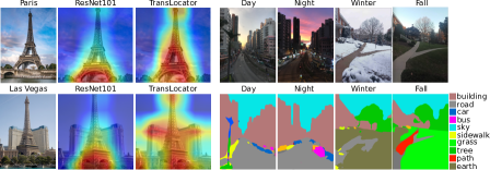
In contrast to many other vision applications, single-image geo-localization often depends on fine-grained visual cues present in small regions of an image. In Figure 1, consider the photo of the Eiffel Tower in Paris and its replica in Las Vegas. Even though these two images seem to come from the same location, the buildings and vegetation in the background play a decisive role in distinguishing them. Similarly, in the case of most other images, the global context spanned over the entire image is more important than individual foreground objects in geo-localization. Recently, a few studies [12, 40] comparing vision transformer (ViT) with CNNs have revealed that the early aggregation of global information using self-attention enables transformers to build long-range dependencies within an image. Moreover, higher layers of ViT maintain spatial location information better than CNNs. Hence, we argue that transformer-based networks are more effective than CNNs for geo-localization because they focus on detailed visual cues present in the entire image.
Another challenge of single-image geo-localization is the drastic appearance variation of the exact location under different daytime or weather conditions. Semantic segmentation offers a solution to this problem by generating robust representations in such extreme variations [48]. For example, consider the drastic disparity of the RGB images of same locations in day and night or winter and fall in Figure 1. In contrast to the RGB images, the semantic segmentation maps remain almost unchanged. Furthermore, semantic segmentation provides auxiliary information about the objects present in the image. This additional information can be a valuable pre-processing step since it enables the model to learn which objects occur more frequently in which geographic locations. For example, as soon as the semantic map detects mountains, the model immediately eliminates all flat regions, thus, reducing the complexity of the problem.
Planet-scale geo-localization deals with a diverse set of input images caused by different environmental settings (e.g., outdoors vs indoors), which entails different features to distinguish between them. For example, to geo-locate outdoor images, features such as the architecture of buildings or the type of vegetation are important. In contrast, for indoor images, the shape and style of furniture may be helpful. To address such variations, Muller et al. [35] proposed to train different networks for different environmental settings. Though such an approach produces good results, they are cost-prohibitive and are not generalizable to a higher number of environmental scenarios. In contrast, we propose a unified multi-task framework for simultaneous geo-localization and scene recognition applied to images from all environmental settings.
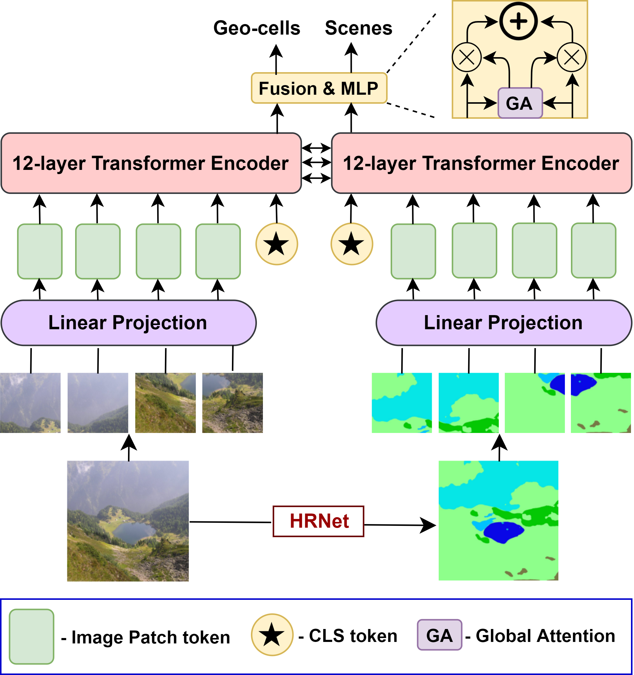
This work addresses the challenges of planet-scale single-image geo-localization by designing a novel dual-branch transformer architecture, TransLocator. We treat the problem as a classification task [35, 65] by subdividing the earth’s surface into a high number of geo-cells and assigning each image to one geo-cell. TransLocator takes an RGB image and its corresponding semantic segmentation map as input, divides them into non-overlapping patches, flattens the patches, and feeds them into two parallel transformer encoder modules to simultaneously predict the geo-cell and recognize the environmental scene in a multi-task framework. The two parallel transformer branches interact after every layer, ensuring an efficient fusion strategy. The resulting features learned by TransLocator are robust under appearance variation and focus on tiny details over the entire image.
In summary, our contributions are three-fold. We propose TransLocator - a unified solution to planet-scale single-image geo-localization with a dual-branch transformer network. TransLocator is able to distinguish between similar images from different locations by precisely attending to tiny visual cues. We propose a simple yet efficient fusion of two transformer branches, which helps TransLocator to learn robust features under extreme appearance variation. We achieve state-of-the-art performance on four datasets with a significant improvement of , , , continent-level geolocational accuracy on ImGPS [17], ImGPSk [18], YFCCk [61], and YFCCk [53], respectively. We also qualitatively evaluate the effectiveness of the proposed method on real-world images. Our source code is available at https://github.com/ShramanPramanick/Transformer_Based_Geo-localization.
2 Related Works
2.1 Single-image geo-localization
Small-scale approaches: Planet-scale single-image geo-localization is difficult due to several challenges, including the large variety of images due to different environmental scenarios and drastic differences in the appearance of same location based on the weather, time of day, or season. For this reason, many existing approaches are limited to geo-locating images captured in very specific and constrained locations. For example, many approaches have been restricted to geo-locating an image within a single city [48, 16, 3], such as Pittsburgh [58], San Francisco [8], or Tokyo [57]. Far fewer approaches have attempted geo-localization in natural, non-urban environments. Some have limited the problem to only very specific natural environments, such as beaches [5, 63], deserts [59], or mountains [2, 45].
Cross-view approaches: The challenge of large-scale image geo-localization with few landmarks and limited training data has led some researchers to propose cross-view approaches, which match a query ground-level RGB image with a large reference dataset of aerial or satellite images [29, 55, 21, 42, 56, 81, 69, 80]. However, these approaches require access to a relevant reference dataset which is not available for many locations.
Planet-scale approaches: Only a few approaches have attempted to geo-locate images on a scale of an entire world without any restrictions. ImGPS [17] was the first work to geo-locate images taken anywhere on the earth using hand-crafted features and nearest neighbor search. The same authors have later improved their approach [18] by refining the search with multi-class support vector machines. PlaNet [65] was the first deep learning approach for unconstrained geo-localization which significantly outperformed the two ImGPS approaches [17, 18]. Vo et al. [61] combined the ImGPS and PlaNet approaches by using the deep-learning-based features to match a query image with a nearest neighbors search. The approach by Muller et al. [35] achieved the current state-of-the-art performance for unconstrained geo-localization. They fine-tuned three separate ResNet networks, each trained only on images of outdoor natural, outdoor urban, or indoor scenes. Detailed surveys of existing work on geo-localization can be found at [4, 33].
2.2 Vision Transformer
Following the success of transformers [60] in machine translation, convolution-free networks that rely only on self-attentive transformer layers have gone viral in computer vision. In particular, Vision Transformer (ViT) [13] was the first to apply a pure transformer architecture on non-overlapping image patches and surpassed CNNs for image classification. Inspired by ViT, transformers have been widely adopted for various computer vision tasks, such as object detection [6, 82, 14, 27], image segmentation [66, 76, 49, 10], video understanding [71, 50, 64, 67], low-shot learning [12, 73], image super resolution [68, 9], D classification [75, 34], and multimodal learning [32, 28, 24, 26, 1, 20, 70].
We are the first to address the ill-posed planet-scale single-image geo-localization problem by designing a novel dual-branch transformer architecture. Unlike [35], we use only a single network for all kinds of input images, allowing our model to take advantage of the similar features from different scenes while maintaining its ability to learn scene-specific features. Moreover, our approach is robust under extreme appearance variations and generalizes to challenging real-world images.
3 Proposed System - TransLocator
This section presents our proposed multimodal multi-task system, TransLocator for geo-location estimation and scene recognition. Following the literature [65, 47, 35], we treat geo-localization as a classification problem by subdividing the earth into several geographical cells111Following [35], we use the S geometry library to generate the geo-cells. containing a similar number of images. As the size and the number of geo-cells poses a trade-off between system performance and classification difficulty, we use multiple partitioning schemes which allow the system to learn geographical features at different scales, leading to a more discriminative classifier. Furthermore, we incorporate semantic representations of RGB images to learn robust feature representation across different daytime and weather conditions. Finally, we predict the geo-cell and environmental scenario of the input image by exploiting contextual information in a multi-task fashion.
3.1 Global Context with Vision Transformer
We use a vision transformer (ViT) [13] model as the backbone of our architecture. Transformers have traditionally been used for sequential data, such as text or audio [60, 37, 11, 72, 30]. In order to extend transformers to vision problems, an image is split into a sequence of -D patches which are then flattened and fed into the stacked transformer encoders through a trainable linear projection layer. An additional classification token (CLS) is added to the sequence, as in the original BERT approach [11]. Moreover, positional embeddings are added to each token to preserve the order of the patches in the original image. A transformer encoder is made up with a sequence of blocks containing multi-headed self-attention (MSA) with a feed-forward network (FFN). FFN contains two multi-layer perceptron (MLP) layers with GELU non-linearity applied after the first layer. Layer normalization (LN) is applied before every block, and residual connections after every block. The output of -th block in the transformer encoder can be expressed as
| (1) |
| (2) |
| (3) |
where is the CLS token, is the patch tokens at -th layer, and is the positional embeddings. and is the patch-sequence length and embedding dimension, respectively. denotes concatenation.
The self-attention in ViT is a mechanism to aggregate information from all spatial locations and is structurally very different from the fixed-sized receptive field of CNNs. Every layer of ViT can access the whole image and, thus, learn the global structure more effectively. This particular attribute of ViT plays a vital role in our classification system. In agreement with Raghu et al. [40], we empirically establish how the global receptive field of ViT can help to attend to small but essential visual cues, which CNNs often neglect. We provide a detailed comparative evaluation of this phenomenon in Section LABEL:sec:interpretability.
3.2 Semantic Segmentation for Robustness to Appearance Variation
In order to improve the network’s ability to generalize to scenes captured in different daytime and weather conditions, we train a dual-branch vision transformer on the RGB images and their corresponding semantic segmentation maps. As shown in Figure 1, compared to RGB features, the semantic layout of a scene is generally more robust to drastic appearance variations. We use HRNet [62] pre-trained on ADE20K and scene parsing datasets [78, 79] to obtain high resolution semantic maps. HRNet assigns each pixel in the RGB image to one of the pre-defined object classes, such as sky, tree, sea, building, grass, pier, etc.
Multimodal Feature Fusion (MFF): Our proposed framework contains two parallel transformer branches, one for the RGB image and the other for the corresponding semantic map. Since the two branches carry complementary information of the same input, effective fusion is the key for learning multimodal feature representations. We propose a simple and computationally light fusion scheme, where we sum the CLS tokens of each branch after every transformer encoder layer. At each layer, the CLS token is considered as an abstract global feature representation. This strategy is as effective as concatenating all feature tokens, but avoids quadratic complexity. Once the CLS tokens are fused, the information will be passed back to patch tokens at the later transformer encoder layers. More formally, , the token sequence at -th layer of a branch can be expressed as
| (4) |
where and are the projection and back-projection functions used to align the dimensions.
Since the relative importance of the two branches depends upon the structure of the input image, we attentively fuse the CLS tokens from the last layer of each branch. Motivated by [15, 39, 38], we design our attention module with two major parts – modality attention generation and weighted concatenation. In the first part, a sequence of dense layers followed by a softmax layer is used to generate the attention scores for the two branches. In the second part, the CLS tokens from the last transformer layer are weighted using their respective attention scores and concatenated together as follows
| (5) |
| (6) |
| (7) |
We use residual connections to improve the gradient flow. The final multimodal representation, , is fed into fully-connected classifier heads.
3.3 Single Model with Multi-Task Learning
Different features are essential for various environmental settings, such as indoor and outdoor urban or natural scenes. Hence, geo-localization can benefit from contextual knowledge about the surroundings, and this information can reduce the complexity of the data space, thus simplifying the classification problem. Muller et al. [35] addressed this issue and approached the problem by fine-tuning three individual networks separately on natural, urban, and indoor images. However, one immediate drawback of their approach is that using multiple separate networks is cost-prohibitive and limits the number of scene kinds. In addition, the separately trained networks can not share the learned features, which likely have semantic similarities across different scene kinds, which effectively reduces the size and potency of the training set.
We address these two drawbacks by training a single network with a multi-task learning objective for simultaneous geo-localization and scene recognition. Following [35], we use a ResNet- pre-trained on Places dataset222Places ResNet model: https://github.com/CSAILVision/places365 [77] to label the training images with corresponding different scene categories. Additionally, based on the provided scene hierarchy333http://places2.csail.mit.edu/download.html, we label each image with a coarser and different scene labels. In multi-task learning, adding complementary tasks has been proven to improve the results of the main task [7, 41, 74]. We follow a multi-task learning approach known as hard parameter sharing [44] which shares the parameters of hidden layers for all tasks and uses task-specific classifier heads. This strategy reduces overfitting because learning the same weights for multiple tasks forces the model to learn a generalized representation useful for the different tasks. More specifically, we only add a classifier head on top of the fused multimodal features and train the system end-to-end for both tasks.
3.4 Training Objective
Since there is a trade-off between the classification difficulty and the prediction accuracy caused by the number and size of the geo-cells, we use partitioning of the earth’s surface at three different resolutions, which we call coarse, middle and fine geo-cells444Details on geo-cell partitioning can be found in the supplementary material.. We feed the final multimodal feature representation into four parallel classifier heads for the final classification: three for geo-cell prediction and one for scene recognition. We use a cross-entropy loss for each head. Our overall loss function can be summarized as follows:
| (8) |
4 Experiments
We conduct extensive experiments to show the effectiveness of our proposed method. In this section, we describe the datasets, the evaluation metrics, the baseline methods, and the detailed experimental settings.
4.1 Datasets
We use publicly available RGB image datasets with corresponding ground truth GPS (latitude, longitude) tags for training, validation, and testing. We trained our model on the MediaEval Placing Task dataset (MP-) [25] containing M geo-tagged images sourced from Flickr. Like Vo et al. [61], during training we excluded images taken by the same authors in our validation or test sets. We validated and tested our model on two randomly sampled subsets of images from the Yahoo Flickr Creative Commons Million dataset (YFCCM) [54], referred to as YFCCk [53] and YFCCk [61] containing and images, respectively. Since the images of MP-, YFCCk and YFCCk were sourced without any scene and user restrictions, these datasets contain images of landmarks and landscapes, but also ambiguous images with little to no geographical cues, such as photographs of food and portraits of people.
We have additionally tested our model on two smaller datasets commonly used for geo-localization – ImGPS [17] and ImGPSk [18]. ImGPS contains manually selected geo-localizable images. In contrast to the previous three datasets, ImGPS is specially designed to evaluate geo-localization systems and contains images from popular landmarks and famous tourist locations. ImGPSk is an extended version of ImGPS. ImGPSk contains images with geo-tags. Unlike ImGPS, this dataset was not manually filtered and hence, it is a slightly more challenging test compared to ImGPS.
4.2 Baselines
We compare our method to several existing geo-estimation methods, including ImGPS [17], [L]kNN [61], MvMF [23], Planet [65], CPlanet [47], and ISNs [35]. ISNs reports the state-of-the-art results on ImGPS and ImGPSk. More details about the baselines are provided in the supplementary materials. Since neither of the baselines reported their performance on all considered test sets, we re-implement the missing ones. We also provide a detailed ablation study of our method by removing one component at a time from TransLocator in Table 5.
4.3 Evaluation Metrics
We evaluate the performance of our approach using geolocational accuracy at multiple error levels, i.e. the percentage of images correctly localized within a predefined distance from the ground truth GPS coordinates [65, 47, 35]. Formally, if the predicted and ground truth coordinates are and , the geo-locational accuracy at scale (in km) is defined as follows for a set of samples:
| (9) |
where GCD is the great circle distance and = is an indicator function whether the distance is smaller than the tolerated radius . We report the results at km, km, km, km, and km ranges from the ground truth, which correspond to the scale of the same street, city, region, country, and continent, respectively [65].
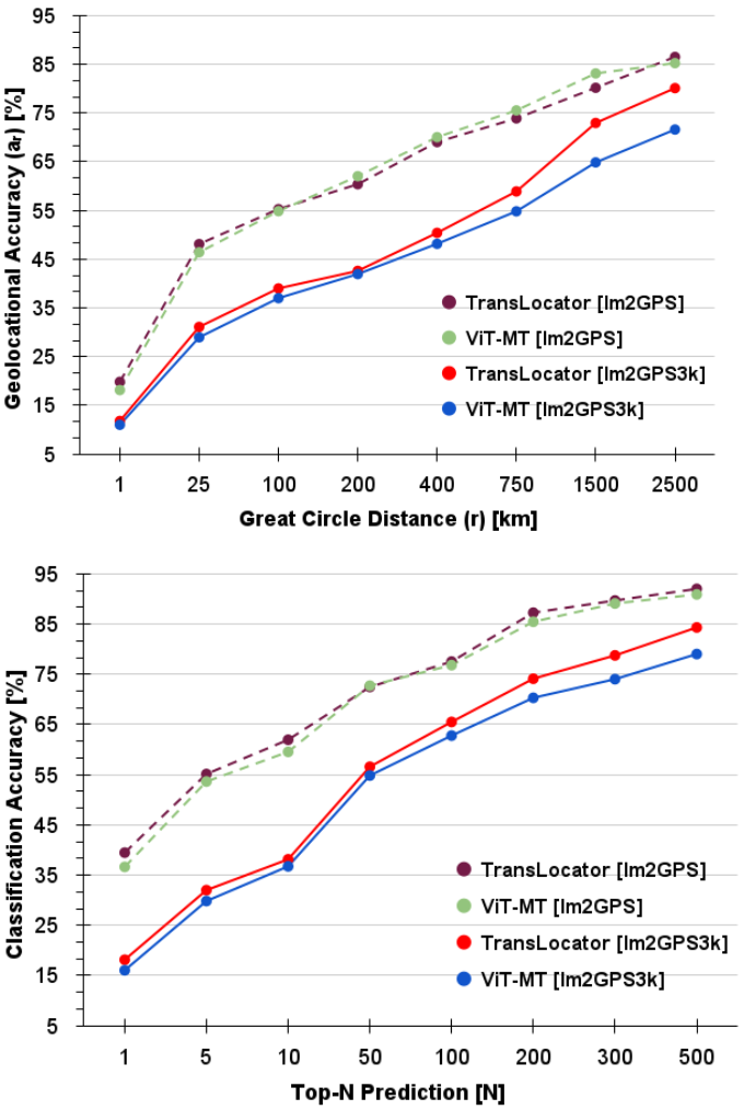
Following Muller et al. [35], we assign the predicted geo-cell a GPS tag by using the mean locations of all training images in that cell. Since the models are trained in a classification framework and evaluated using a distance metric, we empirically verified a strong linear relationship between classification and geo-locational accuracy. The average Pearson correlation coefficient between these two metrics on ImGPS and ImGPSk test sets for TransLocator is , which implies the validity of the classification framework for geo-localization (see Figure 3). More details regarding the strong correlation between these two metrics can be found in the supplementary material.
4.4 Implementation Details
We use ViT-B/ [13] as the backbone of both RGB and segmentation channels. While training a single-channel (RGB only) multi-task transformer network, which we denote as ViT-MT, we use the pre-trained weights on the large ImageNetK [43] dataset containing million images and thousand classes. We fine-tuned it for the geo-localization task. Both channels of the dual-branch TransLocator system are initialized with the weights of the ViT-MT backbone trained for epochs. The weights of the classifier heads are randomly initialized with a zero-mean Gaussian distribution with a standard deviation of . Following the standard ViT literature, we linearly project the non-overlapping patches of pixels for both channels, and we add the CLS token and the positional embeddings.
Since the training set contains images in various resolutions and scales, we use extensive data augmentation, as detailed in the supplementary materials. We implement the methods in Pytorch [36] framework. Our ViT-MT and TransLocator took / days to train on NVIDIA RTX 3090 GPUs, respectively, with GB dedicated memory in each GPU. We train both systems using a AdamW [31] optimizer with an base learning rate of , a momentum of , and a weight decay of . We train the network for a total of epochs with a batch size of . During testing, we convert the fine geo-cells to corresponding GPS coordinates. Other necessary hyper-parameters and data augmentation details are given in the supplementary materials.
| Dataset | Method | Distance ( [%] @ km) | ||||
|---|---|---|---|---|---|---|
| Street | City | Region | Country | Continent | ||
| km | km | km | km | km | ||
| ImGPS [18] | Human [61] | 3.8 | 13.9 | 39.3 | ||
| [L]kNN, = [61] | 14.4 | 33.3 | 47.7 | 61.6 | 73.4 | |
| MvMF [23] | 8.4 | 32.6 | 39.4 | 57.2 | 80.2 | |
| PlaNet [65] | 8.4 | 24.5 | 37.6 | 53.6 | 71.3 | |
| CPlaNet [47] | 16.5 | 37.1 | 46.4 | 62.0 | 78.5 | |
| ISNs (M, f, S3) [35] | 16.5 | 42.2 | 51.9 | 66.2 | 81.0 | |
| ISNs (M,f∗,S3) [35] | 16.9 | 43.0 | 51.9 | 66.7 | 80.2 | |
| \cdashline2-7 | ViT-MT | 18.2 | 46.4 | 62.1 | 74.5 | 85.2 |
| TransLocator | 19.9 | 48.1 | 64.6 | 75.6 | 86.7 | |
| 3.0 | 5.1 | 12.7 | 8.9 | 5.5 | ||
| ImGPS k [17] | [L]kNN, = [61] | 7.2 | 19.4 | 26.9 | 38.9 | 55.9 |
| PlaNet† [65] | 8.5 | 24.8 | 34.3 | 48.4 | 64.6 | |
| CPlaNet [47] | 10.2 | 26.5 | 34.6 | 48.6 | 64.6 | |
| ISNs (M, f, S3) [35] | 10.1 | 27.2 | 36.2 | 49.3 | 65.6 | |
| ISNs (M,f∗,S3) [35] | 10.5 | 28.0 | 36.6 | 49.7 | 66.0 | |
| \cdashline2-7 | ViT-MT | 11.0 | 29.0 | 42.6 | 54.8 | 71.6 |
| TransLocator | 11.8 | 31.1 | 46.7 | 58.9 | 80.1 | |
| 1.3 | 3.1 | 6.1 | 9.2 | 14.1 | ||
| YFCC [53] | [L]kNN, = [61] | 2.3 | 5.7 | 11.0 | 23.5 | 42.0 |
| PlaNet† [65] | 5.6 | 14.3 | 22.2 | 36.4 | 55.8 | |
| CPlaNet [47] | 7.9 | 14.8 | 21.9 | 36.4 | 55.5 | |
| ISNs (M, f, S3)‡ [35] | 6.5 | 16.2 | 23.8 | 37.4 | 55.0 | |
| ISNs (M,f∗,S3)‡ [35] | 6.7 | 16.5 | 24.2 | 37.5 | 54.9 | |
| \cdashline2-7 | ViT-MT | 8.1 | 18.0 | 26.2 | 40.0 | 59.9 |
| TransLocator | 8.4 | 18.6 | 27.0 | 41.1 | 60.4 | |
| 0.5 | 3.8 | 5.1 | 4.7 | 4.9 | ||
| 1.7 | 2.1 | 2.8 | 3.6 | 5.5 | ||
| YFCC k [61] | PlaNet‡ [65] | 4.4 | 11.0 | 16.9 | 28.5 | 47.7 |
| ISNs (M, f, S3)‡ [35] | 5.3 | 12.1 | 18.8 | 31.8 | 50.6 | |
| ISNs (M, f∗, S3)‡ [35] | 5.3 | 12.3 | 19.0 | 31.9 | 50.7 | |
| \cdashline2-7 | ViT-MT | 6.9 | 17.3 | 27.5 | 40.5 | 59.5 |
| TransLocator | 7.2 | 17.8 | 28.0 | 41.3 | 60.6 | |
| 1.9 | 5.5 | 9.0 | 9.4 | 9.9 | ||
5 Results, Discussions and Analysis
In this section, we compare the performance of TransLocator system with different baselines, and conduct a detailed ablation study to demonstrate the importance of different components in our system. Furthermore, we visualize the interpretability of TransLocator using Grad-CAM [46] and perform an error analysis.
| Dataset | Method | Distance ( [%] @ km) | ||||
|---|---|---|---|---|---|---|
| Street | City | Region | Country | Continent | ||
| km | km | km | km | km | ||
| ImGPS [18] | ResNet101 | 14.3 | 41.4 | 51.9 | 64.1 | 78.9 |
| EfficientNet-B4 | 15.4 | 42.7 | 52.8 | 64.8 | 79.5 | |
| ViT base | 16.9 | 43.4 | 54.5 | 67.8 | 80.7 | |
| + Seg | 17.6 | 44.8 | 58.9 | 70.0 | 83.3 | |
| + Seg + MFF | 19.0 | 47.2 | 62.7 | 73.5 | 85.7 | |
| + Seg + MFF + Scene | 19.9 | 48.1 | 64.6 | 75.6 | 86.7 | |
| ImGPS k [18] | ResNet101 | 9.0 | 25.1 | 32.8 | 46.1 | 63.5 |
| EfficientNet-B4 | 9.2 | 26.8 | 32.7 | 47.0 | 63.9 | |
| ViT base | 9.9 | 28.0 | 37.8 | 54.2 | 70.7 | |
| + Seg | 10.5 | 29.1 | 42.5 | 55.8 | 73.6 | |
| + Seg + MFF | 11.1 | 30.2 | 45.0 | 56.8 | 78.1 | |
| + Seg + MFF + Scene | 11.8 | 31.1 | 46.7 | 58.9 | 80.1 | |
5.1 Comparison with Baselines
Table 4.4 presents the performance of our proposed TransLocator system and baseline methods on all four evaluation datasets. The reported baselines have a similar number of training images and geographic classes, and hence, we can directly compare the results of our system with them. Since the ImGPS and ImGPSk dataset mainly contains images of landmarks and popular tourist locations, the systems yield high accuracy on these two datasets. On ImGPS, even the earlier methods like PlaNet and MvMF surpass human performance considerably. CPlaNet, a combinational geo-partitioning approach, brings a substantial improvement of in street-level accuracy over PlaNet. A similar trend of results is seen in the case of ImGPSk. On this dataset, CPlaNet beats PlaNet by street-level accuracy. For other distance scales, the results improve proportionally. The Individual Scene Networks (ISNs) report the state-of-the-art result on both of these datasets, achieving and street-level accuracy on ImGPS and ImGPSk, respectively. The ensemble of hierarchical classifications (denoted by f∗) improves their results. However, note that none of these methods use semantic maps in their framework. Thus, we first implement the single-branch multi-task ViT-MT model. Interestingly, even this model produces a significant improvement over ISNs for all scales on both datasets, which can be explained by the global context used by ViT architecture. Our final dual-branch TransLocator system improves on top of ViT-MT. Overall, we push the current state-of-the-art by and street-level and and continent-level accuracy on ImGPS and ImGPSk, respectively.
The YFCCk and YFCCk datasets contain more challenging samples which have little to no geo-locating cues. However, these large datasets of unconstrained real-world images examine the generalizability of the systems. On YFCCk, CPlaNet produces the best street-level accuracy among baselines, while ISNs beats CPlaNet at the continent level. Our proposed TransLocator outperforms both CPlaNet and ISNs in every distance scale, improving the state-of-the-art by and street-level and continent-level accuracy. The YFCCk dataset is even more challenging than YFCCk; the best baseline produces only street-level accuracy. However, our proposed TransLocator system yields an impressive street-level accuracy on YFCCk, which proves the appreciable generalizability of TransLocator.
Acknowledgement: This research is partially supported by an ARO MURI Grant No. WNF---.
References
- [1] Akbari, H., Yuan, L., Qian, R., Chuang, W.H., Chang, S.F., Cui, Y., Gong, B.: Vatt: Transformers for multimodal self-supervised learning from raw video, audio and text. Advances in Neural Information Processing Systems 34, 24206–24221 (2021)
- [2] Baatz, G., Saurer, O., Köser, K., Pollefeys, M.: Large scale visual geo-localization of images in mountainous terrain. In: European Conference on Computer Vision. pp. 517–530. Springer (2012)
- [3] Berton, G., Masone, C., Caputo, B.: Rethinking visual geo-localization for large-scale applications. In: Proceedings of the IEEE/CVF Conference on Computer Vision and Pattern Recognition. pp. 4878–4888 (2022)
- [4] Brejcha, J., Čadík, M.: State-of-the-art in visual geo-localization. Pattern Analysis and Applications 20(3), 613–637 (2017)
- [5] Cao, L., Smith, J.R., Wen, Z., Yin, Z., Jin, X., Han, J.: Bluefinder: Estimate where a beach photo was taken. In: Proceedings of the 21st International Conference on World Wide Web. pp. 469–470 (2012)
- [6] Carion, N., Massa, F., Synnaeve, G., Usunier, N., Kirillov, A., Zagoruyko, S.: End-to-end object detection with transformers. In: European Conference on Computer Vision. pp. 213–229. Springer (2020)
- [7] Caruana, R.: Multitask learning. Machine learning 28(1), 41–75 (1997)
- [8] Chen, D.M., Baatz, G., Köser, K., Tsai, S.S., Vedantham, R., Pylvänäinen, T., Roimela, K., Chen, X., Bach, J., Pollefeys, M., et al.: City-scale landmark identification on mobile devices. In: Proceedings of the IEEE/CVF Conference on Computer Vision and Pattern Recognition. pp. 737–744 (2011)
- [9] Chen, H., Wang, Y., Guo, T., Xu, C., Deng, Y., Liu, Z., Ma, S., Xu, C., Xu, C., Gao, W.: Pre-trained image processing transformer. In: Proceedings of the IEEE/CVF Conference on Computer Vision and Pattern Recognition. pp. 12299–12310 (2021)
- [10] Cheng, B., Misra, I., Schwing, A.G., Kirillov, A., Girdhar, R.: Masked-attention mask transformer for universal image segmentation. In: Proceedings of the IEEE/CVF Conference on Computer Vision and Pattern Recognition. pp. 1290–1299 (2022)
- [11] Devlin, J., Chang, M.W., Lee, K., Toutanova, K.: BERT: Pre-training of deep bidirectional transformers for language understanding. In: Proceedings of the 2019 Conference of the North American Chapter of the Association for Computational Linguistics: Human Language Technologies, Volume 1 (Long and Short Papers). pp. 4171–4186. Association for Computational Linguistics, Minneapolis, Minnesota (Jun 2019). https://doi.org/10.18653/v1/N19-1423, https://aclanthology.org/N19-1423
- [12] Doersch, C., Gupta, A., Zisserman, A.: Crosstransformers: spatially-aware few-shot transfer. Advances in Neural Information Processing Systems 33, 21981–21993 (2020)
- [13] Dosovitskiy, A., Beyer, L., Kolesnikov, A., Weissenborn, D., Zhai, X., Unterthiner, T., Dehghani, M., Minderer, M., Heigold, G., Gelly, S., et al.: An image is worth 16x16 words: Transformers for image recognition at scale. In: International Conference on Learning Representations (2020)
- [14] Fang, Y., Liao, B., Wang, X., Fang, J., Qi, J., Wu, R., Niu, J., Liu, W.: You only look at one sequence: Rethinking transformer in vision through object detection. Advances in Neural Information Processing Systems 34 (2021)
- [15] Gu, Y., Yang, K., Fu, S., Chen, S., Li, X., Marsic, I.: Hybrid attention based multimodal network for spoken language classification. In: ACL. vol. 2018, p. 2379 (2018)
- [16] Hausler, S., Garg, S., Xu, M., Milford, M., Fischer, T.: Patch-netvlad: Multi-scale fusion of locally-global descriptors for place recognition. In: Proceedings of the IEEE/CVF Conference on Computer Vision and Pattern Recognition. pp. 14141–14152 (2021)
- [17] Hays, J., Efros, A.A.: Im2gps: estimating geographic information from a single image. In: Proceedings of the IEEE/CVF Conference on Computer Vision and Pattern Recognition. pp. 1–8. IEEE (2008)
- [18] Hays, J., Efros, A.A.: Large-scale image geolocalization. In: Multimodal Location Estimation of Videos and Images, pp. 41–62. Springer (2015)
- [19] He, K., Zhang, X., Ren, S., Sun, J.: Deep residual learning for image recognition. In: Proceedings of the IEEE/CVF Conference on Computer Vision and Pattern Recognition. pp. 770–778 (2016)
- [20] Hu, R., Singh, A.: Unit: Multimodal multitask learning with a unified transformer. In: Proceedings of the IEEE/CVF International Conference on Computer Vision. pp. 1439–1449 (2021)
- [21] Hu, S., Feng, M., Nguyen, R.M., Lee, G.H.: Cvm-net: Cross-view matching network for image-based ground-to-aerial geo-localization. In: Proceedings of the IEEE/CVF Conference on Computer Vision and Pattern Recognition. pp. 7258–7267 (2018)
- [22] Ioffe, S., Szegedy, C.: Batch normalization: Accelerating deep network training by reducing internal covariate shift. In: International Conference on Machine Learning. pp. 448–456. PMLR (2015)
- [23] Izbicki, M., Papalexakis, E.E., Tsotras, V.J.: Exploiting the earth’s spherical geometry to geolocate images. In: Joint European Conference on Machine Learning and Knowledge Discovery in Databases. pp. 3–19. Springer (2019)
- [24] Kant, Y., Batra, D., Anderson, P., Schwing, A., Parikh, D., Lu, J., Agrawal, H.: Spatially aware multimodal transformers for textvqa. In: European Conference on Computer Vision. pp. 715–732. Springer (2020)
- [25] Larson, M., Soleymani, M., Gravier, G., Ionescu, B., Jones, G.J.: The benchmarking initiative for multimedia evaluation: Mediaeval 2016. IEEE MultiMedia 24(1), 93–96 (2017)
- [26] Lei, J., Li, L., Zhou, L., Gan, Z., Berg, T.L., Bansal, M., Liu, J.: Less is more: Clipbert for video-and-language learning via sparse sampling. In: Proceedings of the IEEE/CVF Conference on Computer Vision and Pattern Recognition. pp. 7331–7341 (2021)
- [27] Li, L.H., Zhang, P., Zhang, H., Yang, J., Li, C., Zhong, Y., Wang, L., Yuan, L., Zhang, L., Hwang, J.N., et al.: Grounded language-image pre-training. In: Proceedings of the IEEE/CVF Conference on Computer Vision and Pattern Recognition. pp. 10965–10975 (2022)
- [28] Li, X., Yin, X., Li, C., Zhang, P., Hu, X., Zhang, L., Wang, L., Hu, H., Dong, L., Wei, F., et al.: Oscar: Object-semantics aligned pre-training for vision-language tasks. In: European Conference on Computer Vision. pp. 121–137. Springer (2020)
- [29] Lin, T.Y., Belongie, S., Hays, J.: Cross-view image geolocalization. In: Proceedings of the IEEE/CVF Conference on Computer Vision and Pattern Recognition. pp. 891–898 (2013)
- [30] Liu, Y., Ott, M., Goyal, N., Du, J., Joshi, M., Chen, D., Levy, O., Lewis, M., Zettlemoyer, L., Stoyanov, V.: Roberta: A robustly optimized bert pretraining approach. arXiv preprint arXiv:1907.11692 (2019)
- [31] Loshchilov, I., Hutter, F.: Decoupled weight decay regularization. In: International Conference on Learning Representations (2018)
- [32] Lu, J., Batra, D., Parikh, D., Lee, S.: Vilbert: Pretraining task-agnostic visiolinguistic representations for vision-and-language tasks. Advances in Neural Information Processing Systems 32 (2019)
- [33] Masone, C., Caputo, B.: A survey on deep visual place recognition. IEEE Access 9, 19516–19547 (2021)
- [34] Misra, I., Girdhar, R., Joulin, A.: An end-to-end transformer model for 3d object detection. In: Proceedings of the IEEE/CVF International Conference on Computer Vision. pp. 2906–2917 (2021)
- [35] Muller-Budack, E., Pustu-Iren, K., Ewerth, R.: Geolocation estimation of photos using a hierarchical model and scene classification. In: Proceedings of the European Conference on Computer Vision (ECCV). pp. 563–579 (2018)
- [36] Paszke, A., Gross, S., Massa, F., Lerer, A., Bradbury, J., Chanan, G., Killeen, T., Lin, Z., Gimelshein, N., Antiga, L., et al.: Pytorch: An imperative style, high-performance deep learning library. Advances in Neural Information Processing Systems 32 (2019)
- [37] Peters, M., Neumann, M., Iyyer, M., Gardner, M., Clark, C., Lee, K., Zettlemoyer, L.: Deep contextualized word representations. In: Proceedings of the 2018 Conference of the North American Chapter of the Association for Computational Linguistics: Human Language Technologies, Volume 1 (Long Papers). pp. 2227–2237 (2018)
- [38] Pramanick, S., Roy, A., Patel, V.M.: Multimodal learning using optimal transport for sarcasm and humor detection. In: Proceedings of the IEEE/CVF Winter Conference on Applications of Computer Vision. pp. 3930–3940 (2022)
- [39] Pramanick, S., Sharma, S., Dimitrov, D., Akhtar, M.S., Nakov, P., Chakraborty, T.: Momenta: A multimodal framework for detecting harmful memes and their targets. In: Findings of the Association for Computational Linguistics: EMNLP 2021. pp. 4439–4455 (2021)
- [40] Raghu, M., Unterthiner, T., Kornblith, S., Zhang, C., Dosovitskiy, A.: Do vision transformers see like convolutional neural networks? Advances in Neural Information Processing Systems 34 (2021)
- [41] Ranjan, R., Patel, V.M., Chellappa, R.: Hyperface: A deep multi-task learning framework for face detection, landmark localization, pose estimation, and gender recognition. IEEE Transactions on Pattern Analysis and Machine Intelligence 41(1), 121–135 (2017)
- [42] Regmi, K., Shah, M.: Bridging the domain gap for ground-to-aerial image matching. In: Proceedings of the IEEE/CVF International Conference on Computer Vision. pp. 470–479 (2019)
- [43] Ridnik, T., Ben-Baruch, E., Noy, A., Zelnik-Manor, L.: Imagenet-21k pretraining for the masses. arXiv preprint arXiv:2104.10972 (2021)
- [44] Ruder, S.: An overview of multi-task learning in deep neural networks. arXiv preprint arXiv:1706.05098 (2017)
- [45] Saurer, O., Baatz, G., Köser, K., Pollefeys, M., et al.: Image based geo-localization in the alps. International Journal of Computer Vision 116(3), 213–225 (2016)
- [46] Selvaraju, R.R., Cogswell, M., Das, A., Vedantam, R., Parikh, D., Batra, D.: Grad-cam: Visual explanations from deep networks via gradient-based localization. In: Proceedings of the IEEE/CVF International Conference on Computer Vision. pp. 618–626 (2017)
- [47] Seo, P.H., Weyand, T., Sim, J., Han, B.: Cplanet: Enhancing image geolocalization by combinatorial partitioning of maps. In: Proceedings of the European Conference on Computer Vision (ECCV). pp. 536–551 (2018)
- [48] Seymour, Z., Sikka, K., Chiu, H.P., Samarasekera, S., Kumar, R.: Semantically-aware attentive neural embeddings for image-based visual localization. arXiv preprint arXiv:1812.03402 (2018)
- [49] Strudel, R., Garcia, R., Laptev, I., Schmid, C.: Segmenter: Transformer for semantic segmentation. In: Proceedings of the IEEE/CVF International Conference on Computer Vision. pp. 7262–7272 (2021)
- [50] Sun, C., Myers, A., Vondrick, C., Murphy, K., Schmid, C.: Videobert: A joint model for video and language representation learning. In: Proceedings of the IEEE/CVF International Conference on Computer Vision. pp. 7464–7473 (2019)
- [51] Szegedy, C., Liu, W., Jia, Y., Sermanet, P., Reed, S., Anguelov, D., Erhan, D., Vanhoucke, V., Rabinovich, A.: Going deeper with convolutions. In: Proceedings of the IEEE/CVF Conference on Computer Vision and Pattern Recognition. pp. 1–9 (2015)
- [52] Tan, M., Le, Q.: Efficientnet: Rethinking model scaling for convolutional neural networks. In: International Conference on Machine Learning. pp. 6105–6114. PMLR (2019)
- [53] Theiner, J., Müller-Budack, E., Ewerth, R.: Interpretable semantic photo geolocation. In: Proceedings of the IEEE/CVF Winter Conference on Applications of Computer Vision. pp. 750–760 (2022)
- [54] Thomee, B., Shamma, D.A., Friedland, G., Elizalde, B., Ni, K., Poland, D., Borth, D., Li, L.J.: Yfcc100m: The new data in multimedia research. Communications of the ACM 59(2), 64–73 (2016)
- [55] Tian, Y., Chen, C., Shah, M.: Cross-view image matching for geo-localization in urban environments. In: Proceedings of the IEEE/CVF Conference on Computer Vision and Pattern Recognition. pp. 3608–3616 (2017)
- [56] Toker, A., Zhou, Q., Maximov, M., Leal-Taixé, L.: Coming down to earth: Satellite-to-street view synthesis for geo-localization. In: Proceedings of the IEEE/CVF Conference on Computer Vision and Pattern Recognition. pp. 6488–6497 (2021)
- [57] Torii, A., Arandjelovic, R., Sivic, J., Okutomi, M., Pajdla, T.: 24/7 place recognition by view synthesis. In: Proceedings of the IEEE/CVF Conference on Computer Vision and Pattern Recognition. pp. 1808–1817 (2015)
- [58] Torii, A., Sivic, J., Pajdla, T., Okutomi, M.: Visual place recognition with repetitive structures. In: Proceedings of the IEEE/CVF Conference on Computer Vision and Pattern Recognition. pp. 883–890 (2013)
- [59] Tzeng, E., Zhai, A., Clements, M., Townshend, R., Zakhor, A.: User-driven geolocation of untagged desert imagery using digital elevation models. In: Proceedings of the IEEE/CVF Conference on Computer Vision and Pattern Recognition Workshops. pp. 237–244 (2013)
- [60] Vaswani, A., Shazeer, N., Parmar, N., Uszkoreit, J., Jones, L., Gomez, A.N., Kaiser, Ł., Polosukhin, I.: Attention is all you need. In: Advances in Neural Information Processing Systems. pp. 5998–6008 (2017)
- [61] Vo, N., Jacobs, N., Hays, J.: Revisiting im2gps in the deep learning era. In: Proceedings of the IEEE/CVF International Conference on Computer Vision. pp. 2621–2630 (2017)
- [62] Wang, J., Sun, K., Cheng, T., Jiang, B., Deng, C., Zhao, Y., Liu, D., Mu, Y., Tan, M., Wang, X., et al.: Deep high-resolution representation learning for visual recognition. IEEE Transactions on Pattern Analysis and Machine Intelligence 43(10), 3349–3364 (2020)
- [63] Wang, Y., Cao, L.: Discovering latent clusters from geotagged beach images. In: Advances in Multimedia Modeling, pp. 133–142. Springer (2013)
- [64] Wang, Y., Xu, Z., Wang, X., Shen, C., Cheng, B., Shen, H., Xia, H.: End-to-end video instance segmentation with transformers. In: Proceedings of the IEEE/CVF Conference on Computer Vision and Pattern Recognition. pp. 8741–8750 (2021)
- [65] Weyand, T., Kostrikov, I., Philbin, J.: Planet-photo geolocation with convolutional neural networks. In: European Conference on Computer Vision. pp. 37–55. Springer (2016)
- [66] Xie, E., Wang, W., Yu, Z., Anandkumar, A., Alvarez, J.M., Luo, P.: Segformer: Simple and efficient design for semantic segmentation with transformers. Advances in Neural Information Processing Systems 34 (2021)
- [67] Xu, H., Ghosh, G., Huang, P.Y., Okhonko, D., Aghajanyan, A., Metze, F., Zettlemoyer, L., Feichtenhofer, C.: Videoclip: Contrastive pre-training for zero-shot video-text understanding. In: Proceedings of the 2021 Conference on Empirical Methods in Natural Language Processing. pp. 6787–6800 (2021)
- [68] Yang, F., Yang, H., Fu, J., Lu, H., Guo, B.: Learning texture transformer network for image super-resolution. In: Proceedings of the IEEE/CVF Conference on Computer Vision and Pattern Recognition. pp. 5791–5800 (2020)
- [69] Yang, H., Lu, X., Zhu, Y.: Cross-view geo-localization with layer-to-layer transformer. Advances in Neural Information Processing Systems 34, 29009–29020 (2021)
- [70] Yang, J., Li, C., Zhang, P., Xiao, B., Liu, C., Yuan, L., Gao, J.: Unified contrastive learning in image-text-label space. In: Proceedings of the IEEE/CVF Conference on Computer Vision and Pattern Recognition. pp. 19163–19173 (2022)
- [71] Yang, L., Fan, Y., Xu, N.: Video instance segmentation. In: Proceedings of the IEEE/CVF International Conference on Computer Vision. pp. 5188–5197 (2019)
- [72] Yang, Z., Dai, Z., Yang, Y., Carbonell, J., Salakhutdinov, R.R., Le, Q.V.: Xlnet: Generalized autoregressive pretraining for language understanding. Advances in Neural Information Processing Systems 32 (2019)
- [73] Ye, H.J., Hu, H., Zhan, D.C., Sha, F.: Few-shot learning via embedding adaptation with set-to-set functions. In: Proceedings of the IEEE/CVF Conference on Computer Vision and Pattern Recognition. pp. 8808–8817 (2020)
- [74] Zhang, Y., Yang, Q.: A survey on multi-task learning. IEEE Transactions on Knowledge and Data Engineering (2021)
- [75] Zhao, H., Jiang, L., Jia, J., Torr, P.H., Koltun, V.: Point transformer. In: Proceedings of the IEEE/CVF International Conference on Computer Vision. pp. 16259–16268 (2021)
- [76] Zheng, S., Lu, J., Zhao, H., Zhu, X., Luo, Z., Wang, Y., Fu, Y., Feng, J., Xiang, T., Torr, P.H., et al.: Rethinking semantic segmentation from a sequence-to-sequence perspective with transformers. In: Proceedings of the IEEE/CVF Conference on Computer Vision and Pattern Recognition. pp. 6881–6890 (2021)
- [77] Zhou, B., Lapedriza, A., Khosla, A., Oliva, A., Torralba, A.: Places: A 10 million image database for scene recognition. IEEE Transactions on Pattern Analysis and Machine Intelligence 40(6), 1452–1464 (2017)
- [78] Zhou, B., Zhao, H., Puig, X., Fidler, S., Barriuso, A., Torralba, A.: Scene parsing through ade20k dataset. In: Proceedings of the IEEE/CVF Conference on Computer Vision and Pattern Recognition. pp. 633–641 (2017)
- [79] Zhou, B., Zhao, H., Puig, X., Xiao, T., Fidler, S., Barriuso, A., Torralba, A.: Semantic understanding of scenes through the ade20k dataset. International Journal of Computer Vision 127(3), 302–321 (2019)
- [80] Zhu, S., Shah, M., Chen, C.: Transgeo: Transformer is all you need for cross-view image geo-localization. In: Proceedings of the IEEE/CVF Conference on Computer Vision and Pattern Recognition. pp. 1162–1171 (2022)
- [81] Zhu, S., Yang, T., Chen, C.: Vigor: Cross-view image geo-localization beyond one-to-one retrieval. In: Proceedings of the IEEE/CVF Conference on Computer Vision and Pattern Recognition (CVPR). pp. 3640–3649 (June 2021)
- [82] Zhu, X., Su, W., Lu, L., Li, B., Wang, X., Dai, J.: Deformable detr: Deformable transformers for end-to-end object detection. In: International Conference on Learning Representations (2020)
Where in the World is this Image? Transformer-based Geo-localization in the Wild (Supplementary Material)
In this supplementary material, we provide additional details on geo-cell partitioning, data augmentation, hyper-parameter values, baselines, evaluation metrics and illustrate additional quantitative and qualitative results.
Appendix 0.A Implementation Details Hyper-parameter Values
0.A.1 Adaptive Geo-cell Partitioning
We utilize the S geometry library777https://code.google.com/archive/p/s2-geometry-library/source to divide the earth’s surface into a fixed number of non-overlapping geographic cells. To directly compare our results with baselines, we use the same partitioning approach like [35], where we subdivide the earth’s surface into three resolutions containing , , and geo-cells referred to as coarse, middle, and fine cells, respectively. The partitioning ensures each cell contains at least and at most , , and training images for the coarse, middle, and fine resolution. Limiting the number of training images into a minimum and maximum range per geo-cell gives two advantages. First, the training set does not suffer from class imbalance, which is pivotal for classifying many classes. Second, the geographic areas which are heavily photographed are subdivided into smaller cells, allowing more precise geo-localization of these regions (such as big cities and tourist attractions). However, one drawback of this approach is that many geographic areas have less than the required minimum number of images. Consequently, many locations (such as oceans, remote mountainous regions, deserts, poles) are discarded because of insufficient images. With the minimum range of , the partitioning covers almost of the entire earth’s surface.
In classification-based geo-localization, the number of geo-cells closely relates to the prediction accuracy. In other words, since the predicted GPS coordinates are always the mean location of all training images in the predicted geo-cell, coarse cells often can not produce good street-level accuracy. On the other hand, fine cells improve localization precision by generating smaller geo-cells in highly photographed areas. Figure 0.A.1 shows the improvement of street-level ( km) and city-level ( km) geolocational accuracy by using the predictions from finer cells on four different datasets. Since the continent-level ( km) accuracy is not directly related to the size of cells, it remains almost unchanged with geo-cell resolution variation. Next, we use an ensemble of hierarchical classification using all three resolutions. However, in agreement with [53], this method does not achieve a consistent improvement than considering only fine partitioning. Moreover, the ensemble increases inference time by almost . Following these observations, we use the predictions of the fine geo-cells in all our experiments. We believe that adding a retrieval network after classification would improve the performance by allowing the system to search within the predicted geo-cell. However, this paper does not consider any retrieval extensions for a fair comparison with the baselines.

0.A.2 Data Augmentation
Since the training set contains images in various orientations, resolutions and scales, we use extensive data augmentation. The augmentation policy includes: RandomAffine with degrees (, ), ColorJitter containing brightness, contrast, saturation, hue strength of , , , with a probability of , RandomHorizontalFlip with a probability of , Resize in (, ), Tencrop with size (, ) and standard Normalization. We apply ColorJitter only in the RGB channel. Table 0.A.2 shows an empirical analysis of the effectiveness of different augmentation techniques on training TransLocator. We start with the standard Flip, Resize and Normalization operations. Adding Affine transformation and ColorJitter helps in improving the performance by a tiny margin. However, the TenCrop augmentation shows to have a significant effect, improving street-level accuracy in ImGPS and ImGPSk datasets. Since the important visual cues for geo-localization often reside on the edges of the image, taking multiple crops from different positions and averaging the predictions helps in improving the performance.
| Dataset | Method | Distance ( [%] @ km) | ||||
|---|---|---|---|---|---|---|
| Street | City | Region | Country | Continent | ||
| km | km | km | km | km | ||
| ImGPS [18] | RHF + R + N | 18.8 | 46.2 | 62.8 | 73.6 | 83.6 |
| + RA | 18.8 | 46.5 | 63.1 | 73.8 | 83.8 | |
| + RA + CJ | 19.0 | 46.8 | 63.2 | 74.1 | 84.0 | |
| + RA + CJ + TC | 19.9 | 48.1 | 64.6 | 75.6 | 86.7 | |
| ImGPS k [18] | RHF + R + N | 11.3 | 30.4 | 45.7 | 58.0 | 78.4 |
| + RA | 11.4 | 30.6 | 46.0 | 58.0 | 78.5 | |
| + RA + CJ | 11.4 | 30.8 | 45.9 | 58.2 | 78.7 | |
| + RA + CJ + TC | 11.8 | 31.1 | 46.7 | 58.9 | 80.1 | |
| Hyper-parameters | Notation | Value |
|---|---|---|
| #dim for dense layers in MFF | - | |
| \cdashline1-3 #dim for classification FC | coarse | |
| middle | ||
| fine | ||
| scene | ||
| Training | ||
| Batch-size | - | |
| Epochs | ||
| Optimizer | - | AdamW |
| Loss | - | CE |
| Base learning rate | ||
| Momentum | - | 0.9 |
| Learning rate scheduler | - | Cosine |
| Warmup epochs | - | |
| Weight decay | - | |
0.A.3 Hyper-parameter Details
In Table 0.A.2, we furnish the details of hyper-parameters used during training. Grid search is performed on batch size, learning rate, and the depth of classifier heads to find the best hyper-parameter configuration. The model is evaluated after every epoch on the validation set and the best model was taken to be evaluated on the test set. We use AdamW [31] optimizer with cosine learning rate scheduler and fixed number of warmup steps for optimization without gradient clipping.
Appendix 0.B Baselines
In this section, we provide additional details about the baseline methods. Very few approaches in the literature have attempted to geo-locate images on a scale of an entire world without any restrictions. In the last years, CNNs trained with large-scale datasets have significantly improved the planet-scale geo-localization performance. To the best of our knowledge, we are the first to introduce the effectiveness of fusion transformer architecture for this ill-posed problem. We compare our method with the following baselines:
-
ImGPS [17] is the first to attempt planet-scale geo-localization by using a simple retrieval approach to match a given query image based on a combination of different hand-crafted image descriptors to a reference dataset containing more than M GPS-tagged images. This approach has later been improved [18] by refining the search with multi-class support vector machines.
-
PlaNet [65] is the first deep neural network trained for unconstrained planet-scale geo-localization. More specifically, PlaNet divides the earth in geo-cells and trains an inception [51] network with batch normalization [22] using M geo-tagged images. PlaNet outperforms both versions of ImGPS [17, 18] by a substantial margin.
-
[L]kNN [61] proposes a retrieval-based geo-localization system which combines the ImGPS and PlaNet by using features extracted by CNNs for nearest neighbour search. Though this method uses a -times smaller training set than PlaNet, the retrieval-based approach requires a substantially larger inference time and disk space than classification approaches.
-
CPlaNet [47] develops a combinatorial partitioning algorithm to generate a large number of fine-grained output classes by intersecting multiple coarse-grained partitionings of the earth. This technique allows creating small geo-cells while maintaining sufficient training examples per cell and hence improves the street- and city-level geolocational accuracy by a large margin.
-
MvMF [23] introduces the Mixture of von-Mises Fisher (MvMF) loss function for the classification layer that exploits the earth’s spherical geometry and refines the geographical cell shapes in the partitioning.
-
ISNs [35] reduces the complexity of planet-scale geo-localization problem by leveraging contextual knowledge about environmental scenes. To deal with the huge diversity of images on earth’s surface, this approach trains three different ResNet networks for natural, urban, and indoor scenes, and achieves the current state-of-the-art performance on ImGPS and ImGPSk. However, training different networks is cost-prohibitive and can not be generalized to a larger number of scenes. Our work addresses the limitations of ISNs by training a unified dual-branch transformer network in a multi-task framework and improves the state-of-the-art results by a significant margin.
Appendix 0.C Evaluation Metrics
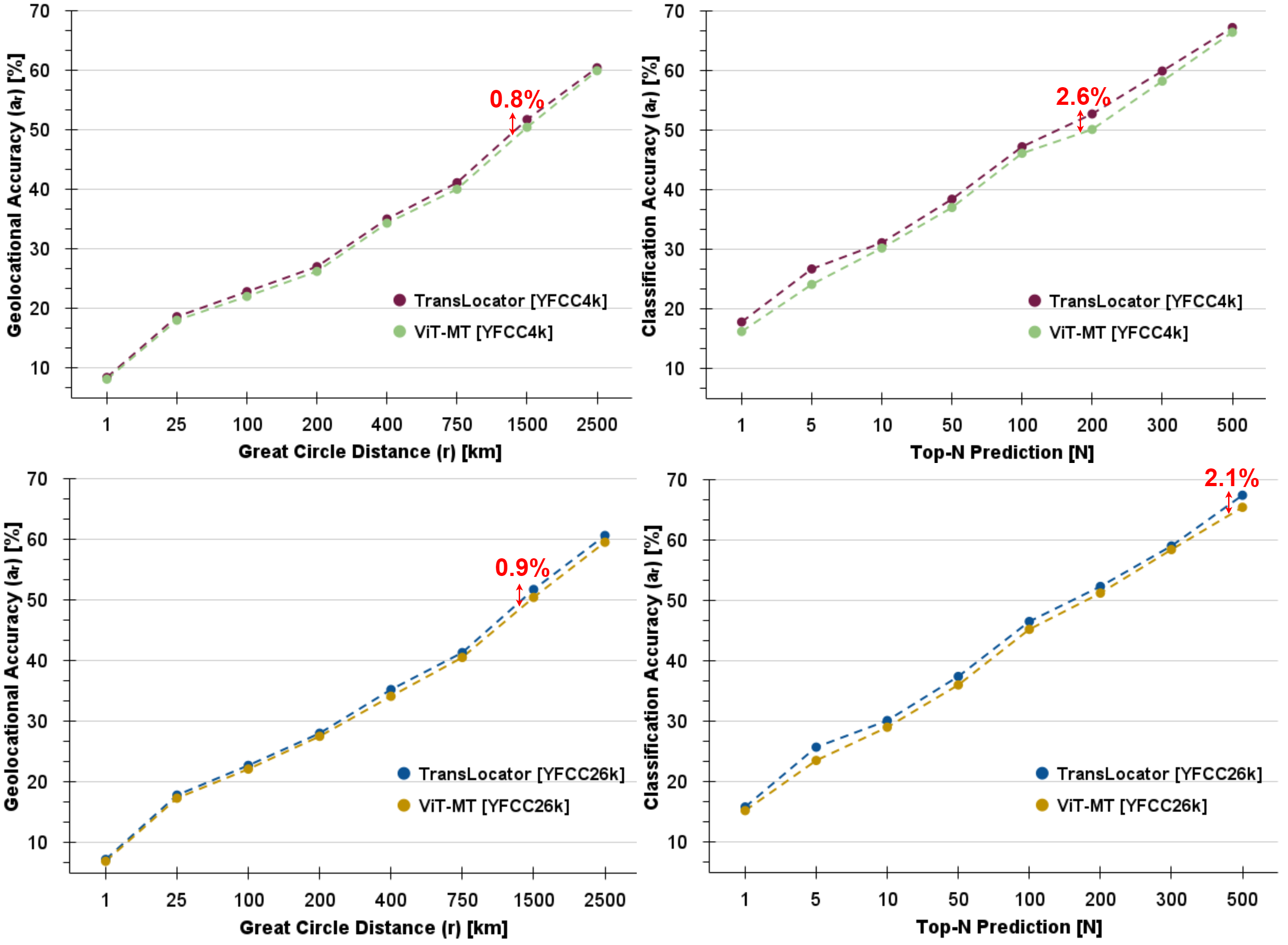
In a classification setup, we train TransLocator using cross-entropy loss which is closely associated with the classification accuracy. However, we evaluate TransLocator using geolocational accuracy. Hence, we empirically verify the strong correlation between these two metrics. We consider the Top- classification accuracy for different values (, , , , , , , ) and geolocational accuracy () for different values (, , , , , , , ) in similar intervals, and observe the correlation among them on different evaluation sets. The Pearson correlation coefficients between the two metrics for TransLocator are , , and on ImGPS, ImGPSk, YFCCk and YFCCk, respectively. We also observe a similarly high correlation for the ViT-MT model. Figure in the main paper and Figure 0.C.1 in supplementary material illustrates the strong linear correlation between the two metrics for TransLocator and ViT-MT on all evaluation sets.
Appendix 0.D Additional Quantitative Results
In this section, we investigate the contribution of different loss functions and provide a direct comparison of TransLocator with the ISNs [35].
0.D.1 Ablation Study on Training Objective
As discussed in section of the main paper, our overall training objective contains three losses for geo-cell prediction and one for scene recognition. Table 0.D.1 shows how each loss function contributes to the performance of TransLocator on ImGPS and ImGPSk datasets. We begin with training TransLocator separately on coarse, middle, and fine geo-cells. As the size of the geo-cells reduces, the geolocational accuracy with a smaller distance threshold typically improves. With the fine geo-cells, TransLocator gains - street-level accuracy than using the coarse cells. Combining all three different geo-cells helps the system learn geographical features at different scales, leading to a more discriminative classifier and improving the street-level accuracy by - . The performance is further improved by another - after adding the scene information, which reduces the complexity of the data space by providing contextual knowledge about the surroundings.
| Dataset | Distance ( [%] @ km) | ||||||||
| Street | City | Region | Country | Continent | |||||
| km | km | km | km | km | |||||
| ImGPS [18] | ✓ | ✗ | ✗ | ✗ | 9.8 | 30.9 | 54.4 | 72.5 | 84.7 |
| ✗ | ✓ | ✗ | ✗ | 14.0 | 38.4 | 58.5 | 72.9 | 86.7 | |
| ✗ | ✗ | ✓ | ✗ | 18.1 | 46.0 | 61.8 | 73.1 | 85.7 | |
| ✓ | ✓ | ✓ | ✗ | 19.0 | 47.2 | 62.7 | 73.5 | 85.7 | |
| ✓ | ✓ | ✓ | ✓ | 19.9 | 48.1 | 64.6 | 75.6 | 86.7 | |
| ImGPS k [18] | ✓ | ✗ | ✗ | ✗ | 5.9 | 22.7 | 40.7 | 54.9 | 77.0 |
| ✗ | ✓ | ✗ | ✗ | 8.0 | 25.5 | 42.8 | 56.9 | 78.1 | |
| ✗ | ✗ | ✓ | ✗ | 10.9 | 29.8 | 45.0 | 56.8 | 78.1 | |
| ✓ | ✓ | ✓ | ✗ | 11.1 | 30.2 | 45.0 | 56.8 | 78.1 | |
| ✓ | ✓ | ✓ | ✓ | 11.8 | 31.1 | 46.7 | 58.9 | 80.1 | |
| Dataset | Method | Train Set {Scene} | Evaluation Set {Scene} (Distance ( [%] @ km) | ||||||||
|---|---|---|---|---|---|---|---|---|---|---|---|
| Natural | Urban | Indoor | |||||||||
| km | km | km | km | km | km | km | km | km | |||
| ImGPS [17] | ISNs (M, f, S3) [35] | Natural | 2.5 | 48.8 | 71.3 | ||||||
| Urban | 22.6 | 56.5 | 89.9 | ||||||||
| Indoor | 15.8 | 31.6 | 57.9 | ||||||||
| \cdashline2-12 | TransLocator w/o scene | Natural | 3.8 | 54.9 | 77.1 | ||||||
| Urban | 24.8 | 65.0 | 88.2 | ||||||||
| Indoor | 20.4 | 55.2 | 79.0 | ||||||||
| \cdashline2-12 | TransLocator | All | 5.0 | 60.8 | 83.8 | 27.5 | 72.9 | 86.9 | 26.3 | 61.4 | 94.7 |
| ImGPS k [18] | ISNs (M, f, S3) [35] | Natural | 3.2 | 31.8 | 63.1 | ||||||
| Urban | 14.1 | 44.8 | 72.7 | ||||||||
| Indoor | 9.2 | 17.8 | 48.4 | ||||||||
| \cdashline2-12 | TransLocator w/o scene | Natural | 4.0 | 36.5 | 70.8 | ||||||
| Urban | 14.4 | 45.9 | 80.2 | ||||||||
| Indoor | 10.4 | 28.2 | 68.5 | ||||||||
| \cdashline2-12 | TransLocator | All | 4.7 | 42.6 | 75.2 | 15.0 | 45.9 | 83.3 | 13.0 | 32.7 | 78.2 |
0.D.2 Differences from ISNs
As the Individual Scene Networks (ISNs) [35] is the first method that utilizes scene information for geo-localization, we present clear differences of our method from ISNs. First, ISNs train three separate ResNet networks for natural, urban and indoor scenes. In contrast, TransLocator uses a unified dual-branch transformer backbone for all scenes. Using three different networks is cost-prohibitive and restricts the system from sharing the learned features across different scene kinds that likely have higher-order semantic similarities. To directly comprehend the effectiveness of a unified network, we train TransLocator without its scene recognition head separately on natural, urban and indoor images. As shown in Table 0.D.1, the single network achieves better performance than separate networks for all three scene kinds. Table 0.D.1 also exhibits the effectiveness of dual-branch transformer backbone than ResNet for geo-localization. Moreover, unlike ISNs, the segmentation branch of TransLocator helps produce better qualitative performance under challenging real-world appearance variation.
Appendix 0.E Additional Qualitative Results
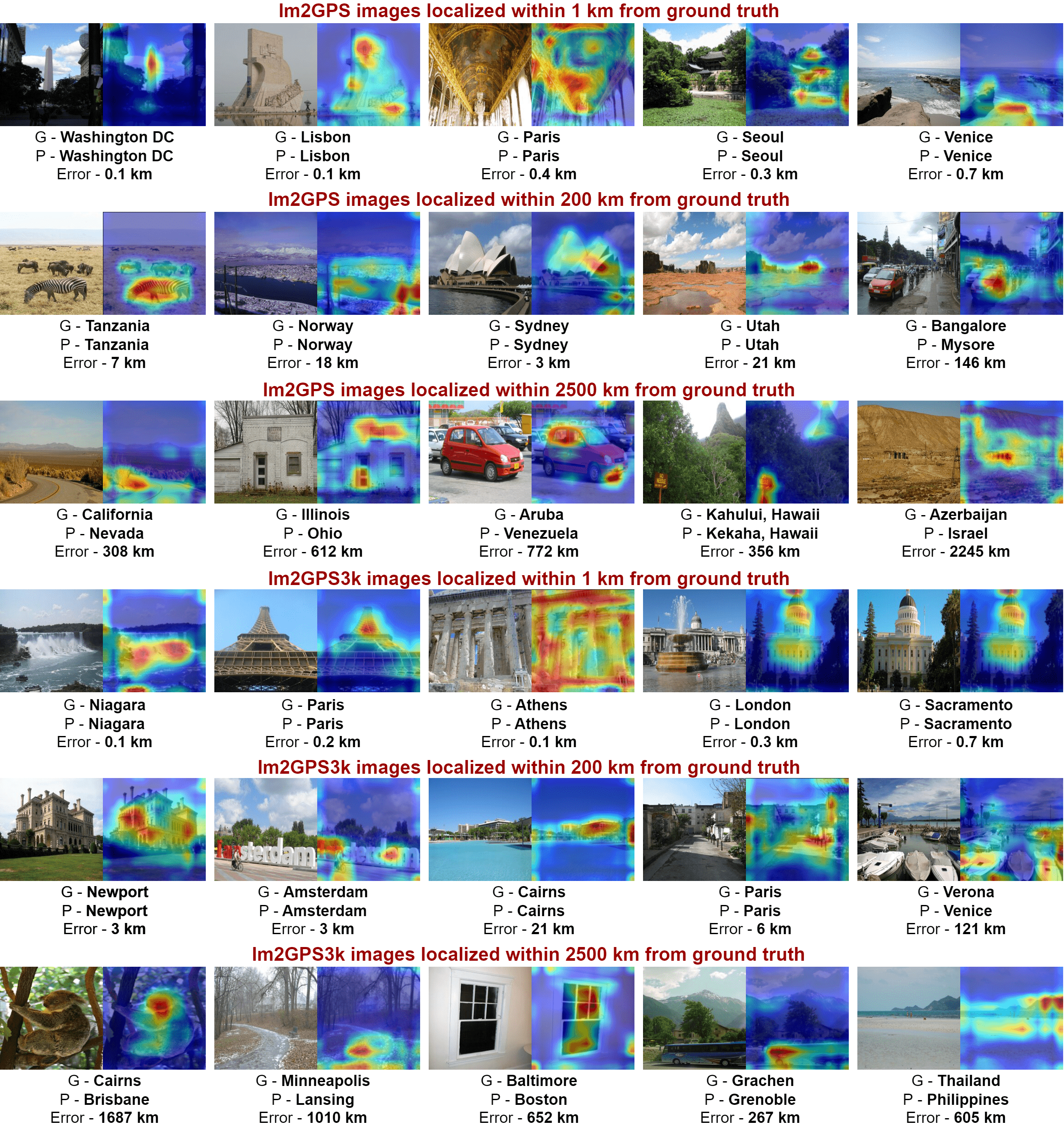
In this section, we visualize a few example images from the ImGPS and ImGPSk datasets localized within km, km, and km from ground truth locations by TransLocator in Figure 0.E.1. The corresponding Grad-CAM [46] activation maps highlight the necessary pixels used for the decision. Famous landmarks and tourist attractions like the Washington Monument, Eiffel Tower, Niagara Falls, and Trafalgar Square are correctly localized. Moreover, TransLocator often yields surprisingly accurate results for images with more subtle geographical cues, like a sea-beach in Venice or a uniquely-shaped building in Seoul. Minor errors like meters occur due to fine cells’ size and can further be removed by using a retrieval extension. More difficult samples, like a forest in Tanzania and a desert in Utah, are localized within a range of - km, which can be attributed to the bigger geo-cells in those sparsely-populated areas. TransLocator can learn to recognize famous streets, buildings, water-bodies, plants, animals and yields surprisingly good results even in remote locations.
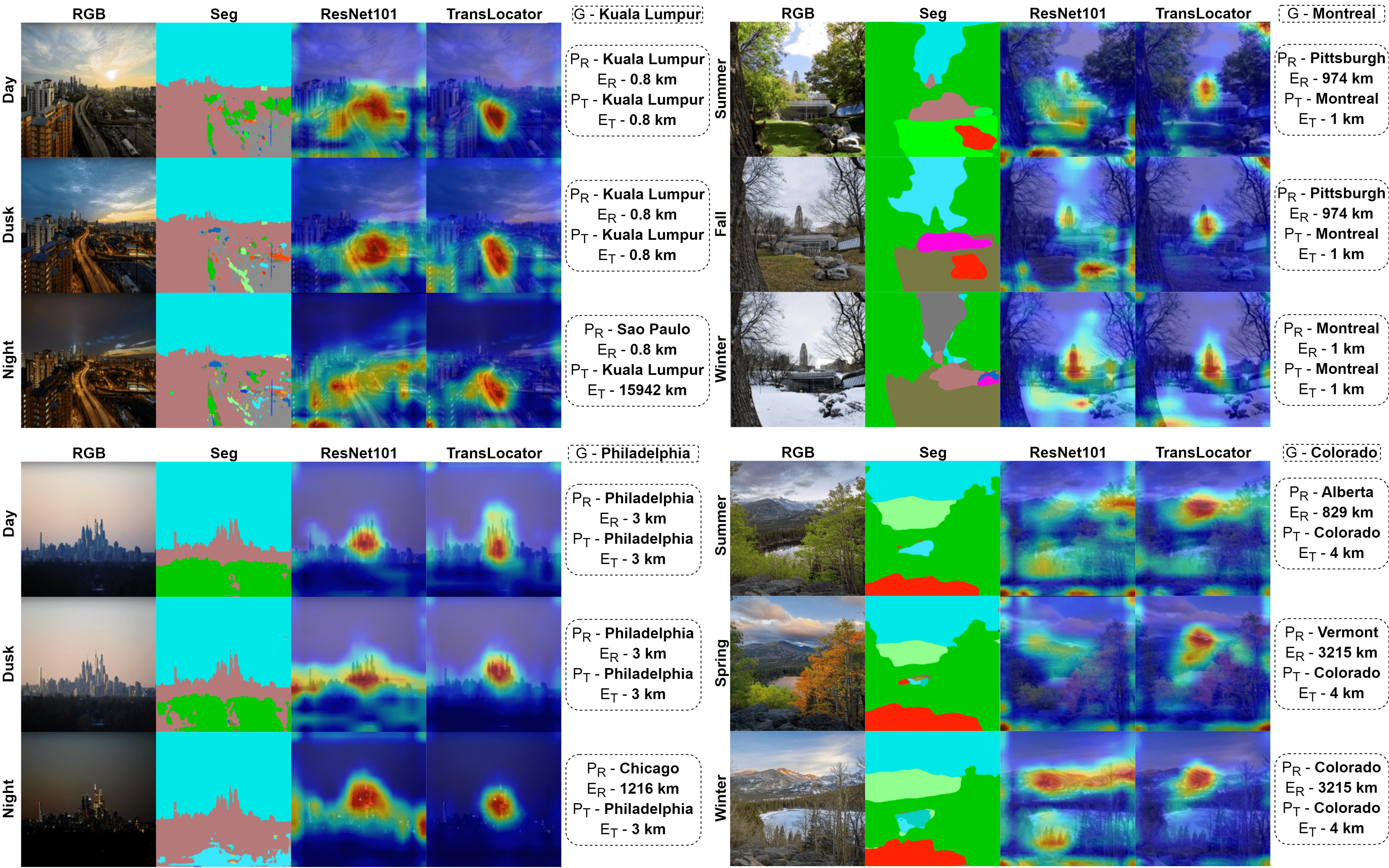
Next, we illustrate a few more cases888Collected from the Internet under creative commons license. of drastic appearance variation in the same location depending on the time of the day, weather, or season in Figure 0.E.2. Though the RGB images experience extreme variation, the corresponding semantic segmentation maps remain unchanged. Thus, TransLocator can learn robust features and produce consistent activation maps across such radical appearance changes. In contrast, ResNet fails to recognize such variation.