A Sampling Control Framework and Applications to Robust and Adaptive Control

Abstract

In this paper, we propose a novel sampling control framework based on the emulation technique where the sampling error is regarded as an auxiliary input to the emulated system. Utilizing the supremum norm of sampling error, the design of periodic sampling and event-triggered control law renders the error dynamics bounded-input-bounded-state (BIBS), and when coupled with system dynamics, achieves global or semi-global stabilization. The proposed framework is then extended to tackle the event-triggered and periodic sampling stabilization for a system where only partial state is available for feedback and the system is subject to parameter uncertainties. The proposed framework is further extended to solve two classes of event-triggered adaptive control problems where the emulated closed-loop system does not admit an input-to-state stability (ISS) Lyapunov function. For the first class of systems with linear parameterized uncertainties, even-triggered global adaptive stabilization is achieved without the global Lipschitz condition on nonlinearities as often required in the literature. For the second class of systems with uncertainties whose bound is unknown, the event-triggered adaptive (dynamic) gain controller is designed for the first time. Finally, theoretical results are verified by two numerical examples.

I Introduction

The majority of modern control relies on its digital implementation in microprocessors and/or is deployed in a networked environment. And the sampled-data control scheme [2, 3] thus arises from the demand of more efficient controller execution to reduce computation cost and save communication bandwidth in applications, such as multi-robot systems, electrical power systems and chemical processes. Sampled-data control schedules the update of a digital controller output at periodic or aperiodic sampling instances. Input-delay approach [12, 11, 10] is usually adopted to design sampled-data controller for linear systems, while two other methods are mainly used for nonlinear systems, namely controller emulation, involving digital implementation of a continuous-time stabilizing control law, and plant discretization consists of discretizing the plant model and discrete-time control law design [21]. However, the sampled-data control approach may over-sample in some cases and motivates event-triggered control which suggests scheduling update only when necessary and specified by the occurrence of the designated triggering event and may achieve more efficient sampling pattern. Sampled-data and event-triggered have been developed for stabilization and tracking of individual systems, e.g., [26, 19, 25, 18] and cooperative control of networked systems, e.g., [9, 23, 5, 29]. In this paper, these two control methods are uniformly called the sampling control.

The two-step digital emulation, constituting continuous-time control law design and its digital implementation, is a common technique for analysis and design of sampling control systems especially for nonlinear systems. In [14, 22], when the emulation of periodic sampled-data control is formulated in the hybrid system setting, the maximum allowable sampling period (MASP) that guarantees asymptotic stability of sampled-data systems can be explicitly computed. In [4], a new small gain theorem is proposed to reveal the quantitative tradeoff between robustness and sampling bandwidth of the sampled-data control. Emulation is also commonly adopted for the design of event-triggered laws where the continuous-time controller is assumed to ensure dissipativity [21] or the input-to-state stability (ISS) of the closed-loop system with the sampling error as input, see, e.g., [1, 7, 18, 20, 17, 25]. The ISS condition can be specified in a max-form, e.g. [18, 30] or in an ISS-Lyapunov form, e.g. [1, 17, 20, 25] for the closed-loop sampling system and the small gain conditions were then proposed to ensure the stability of the event-triggered system. In [16], the event-triggered technique in [25] was interpreted as a stabilization problem of interconnected hybrid systems for which each subsystem admits an ISS-Lyapunov function and a hybrid small gain condition was proposed. As another variant of small gain theorem, the cyclic small gain theorem has been proved effective for event-triggered control of large-scale systems [7, 17, 18].

Achieving Zeno free sampling and robustness to the disturbance and uncertainties simultaneously is not trivial. In [8], a dynamic output-based event-triggered law is proposed to achieve a finite $L_{p}$-gain and a strictly positive lower bound on the inter-event times when the system is subjected to non-vanishing external disturbances. In [18], event-triggered control scheme is designed for systems subject to disturbances. In order to handle the uncertainties, [17] proposed a dynamic event-triggered controller to achieve the stabilization when the system has the dynamic uncertainties whose state is not available for the feedback. The problem is solved in [30] by a static event-triggered controller using a particular small-gain theorem method.

Recently, a few works on the event-triggered adaptive control have been proposed when systems possess parameter uncertainties. Since ISS condition is not guaranteed by the continuous-time stabilization controller and how to design an event-triggered adaptive control scheme is still challenging problem. In [28], an event-triggered adaptive control scheme was proposed for a class of nonlinear systems based on the $\sigma$-modification scheme. $\sigma$-modification scheme results in an ISS Lyapunov function, but only practical stabilization can be achieved, i.e., the trajectories converge to a bounded set in the neighborhood of the origin. The event-triggered law in [28] was improved in [13] in the sense that the adaptation dynamics was also sampled on the assumption of global Lipschitz conditions. In [27], a novel event-triggered adaptive control scheme is proposed for a class of nonlinear systems with unknown control direction and unknown sensor faults, while only practical stabilization is achieved.

In this paper, we propose a novel sampling control framework that can lead to event-triggered and periodic sampling robust and adaptive stabilization of nonlinear systems. The main contribution of this paper is three-fold. First, the paper proposes a sampling control framework where the error caused by the sampling of the actuation is regarded as the auxiliary input to the emulated system. The emulated closed-loop system is first assumed to admit an ISS Lyapunov function when regarding the auxiliary input as the input, while the error dynamics admits an continuously differentiable function whose derivative is bounded by functions of state and sampling errors. The design of periodic sampling and event-triggered control law renders the error dynamics bounded-input-bounded-state (BIBS), when coupled with system dynamics, achieves global or semi-global stabilization. Zeno free behavior is theoretically guaranteed and the system performance is robust to the external disturbances. Second, the proposed framework is then extended to tackle the event-triggered and periodic sampling control for the systems where only partial state is available for the feedback and the system is subject to parameter uncertainties. The proposed controller design combines the method proposed in Section III and changing supply function method. In [18, 17], an auxiliary dynamic system is introduced to estimate the decay rate of immeasurable states and used as the dynamic threshold for the event-triggered law, while the proposed controller is static and easier to design and implement in practice. The periodic sampling control is also proposed here, which is not considered in [18, 17, 30]. Third, the proposed framework is extended to solve two classes of event-triggered adaptive control problems where the emulated closed-loop system does not admit an ISS Lyapunov function. The first class of systems contains linear parameterized uncertainties, and global asymptotical stabilization is achieved without the global Lipschitz condition as often required in [13]. The second class of systems has the uncertainties whose bound is not known and requires adaptive/dynamic gain technique. To author’s best knowledge, the event-triggered dynamic gain control is first time solved in this paper.

The rest of the paper is organized as follows. Section II formulates the sampling control problem for nonlinear systems which will be solved by the sampling control framework proposed in Section III when an ISS condition is assumed. The proposed framework is extended to tackle the event-triggered and periodic sampling control for the systems where only partial state is available for the feedback in Section IV. It is further extended to solve event-triggered adaptive stabilization of two types of uncertain systems in Section V. The numerical simulation is conducted in Section VI and the paper is concluded in Section VII.

Notations. $\mathbb{R}_{\geq 0}$ and $\mathbb{R}_{>0}$ denote the set of non-negative and positive real numbers, respectively. $\mathbb{R}^{n}$ denotes the real space of dimension $n$, $\mathbb{R}^{n\times m}$ denotes the set of real matrices with dimension $n\times m$, and $\mathbb{N}$ denotes the set of non-negative integers. Let $\|x_{[a,b]}\|:=\sup_{t\in[a,b]}\|x(t)\|$ be the supremum norm of a given signal $x:\mathbb{R}_{\geq 0}\mapsto\mathbb{R}^{n}$, over the interval $[a,b]$, and $x_{[a,b]}$ be the signal slice of $x$ over the interval $[a,b]$. Denote a function by $\alpha\in\mathcal{K}_{\infty}$ if it is a $\mathcal{K}_{\infty}$ function, by $\alpha\in\mathcal{KL}$ if it is a $\mathcal{KL}$ function, by $m\in\mathcal{SP}$ if it is a smooth positive function and by $m\in\mathcal{SN}$ if it is a smooth non-negative function. A continuous function $\alpha:[0,\infty)\times(0,\infty)\mapsto[0,\infty)$ is said to be a parameterized $\mathcal{K}_{\infty}$ function if, for each fixed $s>0$, the function $\alpha(\cdot,s)$ is a $\mathcal{K}_{\infty}$ function, and for each fixed $r>0$, the function $\alpha(r,\cdot)$ is non decreasing. For $\mathcal{K}_{\infty}$ functions $\alpha^{\prime}(s)$ and $\alpha(s)$, $\alpha^{\prime}(s)=\mathcal{O}[\alpha(s)]$ as $s\rightarrow 0^{+}$ means that $\lim\sup_{s\rightarrow 0^{+}}[\alpha^{\prime}(s)/\alpha(s)]<\infty$. Let $V:\mathbb{R}^{n}\mapsto\mathbb{R}_{\geq 0}$ be a continuously differentiable function. It is called an ISS-Lyapunov function for the system $\dot{x}=f(x,u,d)$ if the derivative of $V(x)$ along the $x$-dynamics satisfies, for all $x\in\mathbb{R}^{n}$, $\varpi\in\mathbb{R}^{m}$ and $d\in\mathbb{D}$,

$$\underline{\alpha}(\|x\|)\leq V(x)\leq\bar{\alpha}(\|x\|),$$

$$\dot{V}(x)\leq-\alpha(\|x\|)+\sigma(\|\varpi\|)$$ (1)

where $\underline{\alpha},\bar{\alpha},\alpha,\sigma\in\mathcal{K}_{\infty}$. The inequalities in (1) are simplified as $V(x)\sim\{\underline{\alpha},\bar{\alpha},\alpha,\sigma\mid\dot{x}=f(x,u,d)\}$. A bounded piecewise continuous function $f:[0,\infty)\mapsto\mathbb{R}^{n}$ is said to be persistent exciting (PE) if there exist positive constant $\epsilon$, $t_{0}$, $T_{0}$ such that, $\frac{1}{T_{0}}\int_{t}^{t+T_{0}}f(s)f^{\mbox{\tiny{T}}}(s)ds\geq\epsilon^{2}I,\;\forall t\geq t_{0}.$

II Problem Formulation of Sampling Control

Consider the nonlinear system

$$\dot{x}(t) = f(x(t),u(t),d(t)),$$

$$y(t) = h(x(t)),$$ (2)

where $x\in\mathbb{R}^{n}$ is the system state, $y\in\mathbb{R}^{q}$ the output, $u\in\mathbb{R}^{m}$ the control input, and $d\in\mathbb{R}^{n_{d}}$ system uncertainty. Suppose the function $f:\mathbb{R}^{n}\times\mathbb{R}^{m}\times\mathbb{R}^{n_{d}}\mapsto\mathbb{R}^{n}$ is a continuously differentiable function satisfying $f(0,0,d(t))=0$ and $h(0)=0$, and the uncertainty $d$ belongs to a compact set $d\in\mathbb{D}$. Suppose the equilibrium point of the system can be stabilized by a continuous-time feedback controller

$$u(t)=\kappa(y(t)),$$ (3)

with a continuously differentiable function $\kappa$. It becomes a continuous-time state feedback system when $y=x$. In this paper, we use the emulation technique to study the sampling version of (3) as follows

$$u(t) =\kappa(y(t_{k})),\;t\in[t_{k},t_{k+1}),\;k\in\mathbb{N}$$ (4)

where $\{t_{k}\}_{k\in\mathbb{N}}$ is a sequence of sampling time instances. The sampling instances can be determined by an event-triggered law specified as follows

$$t_{k+1}=\inf_{t>t_{k}}\{\Xi(t,t_{k},x_{[t_{k},t]})\geq 0\}$$ (5)

for some functional $\Xi$ representing event occurrence to be designed. A periodic sampling law with sampling period $T>0$ can be considered as a special case of (5) with $\Xi(t,t_{k},x_{[t_{k},t]})=t-t_{k}-T$, i.e., $t_{k+1}=t_{k}+T$. Note that the error caused by the sampling mechanism is

$$\varpi(t):=\kappa\circ h(x(t_{k}))-\kappa\circ h(x(t)),\;t\in[t_{k},t_{k+1}).$$ (6)

For the emulation, the closed-loop system composed of the dynamics (2) and a sampling version of feedback controller (4) is put into the impulsive form

$$\dot{x}=f_{c}(x,\varpi,d):=f(x,\kappa\circ h(x)+\varpi,d),$$

$$\dot{\varpi}=\psi(x,\varpi,d):=-\frac{\partial\kappa\circ h(x)}{\partial x}f_{c}(x,\varpi,d),\forall t\in[t_{k},t_{k+1}),$$

$$\varpi(t_{k}^{+})=0.$$ (7)

The objective of the sampling control is to design the sampling law (5), either periodic sampling or event-triggered law, such that the closed-loop system composed of (2) and (4) achieves two objectives,

1. stabilization: the original system is asymptotically stable at the origin, in particular, $\lim_{t\rightarrow\infty}x(t)=0$, semi-globally or globally;

2. Zeno-free behavior: a finite number of events are triggered in a finite amount of time.

In general, the continuous-time feedback controller in (3) is assumed to ensure that the $x$-subsystem in (7) has some properties such as input-to-state stability (ISS) when regarding sampling error $\varpi$ as the input. The motivation of using the sampling error of the actuation $\varpi$ rather than state or output measurement is explained in [15]. It is exploited in our previous papers [15, 30] to design event-triggered control law where $x$-dynamics is assumed to have the ISS condition specified in a max-form. As is known, the classic analysis tools developed for the adaptive control rely on the Lyapunov function method, typically along the gradient of a Lyapunov function. In order to solve event-triggered adaptive control in Section V, this paper first considers the ISS condition specified in terms of ISS-Lyapunov function and assumes the existence of a positive function on $\varpi$-subsystem which plays a similar role of a Lyapunov function. As a result, the sampling control framework proposed in next section can be naturally extended to event-triggered adaptive control in Section V where the continuous-time adaptive control does not admit an ISS condition.

Assumption II.1

The $x$-subsystem in (7) has an ISS-Lyapunov function $V(x)\sim\{\underline{\alpha},\bar{\alpha},\alpha,\sigma\mid\dot{x}=f_{c}(x,\varpi,d)\}$. There exists a continuously differentiable $U(\varpi):\mathbb{R}^{m}\mapsto\mathbb{R}_{\geq 0}$ such that the derivative of $U(\varpi)$ along the $\varpi$-subsystem, for all $x\in\mathbb{R}^{n}$, $\varpi\in\mathbb{R}^{m}$ and $d\in\mathbb{D}$, satisfies

$$\underline{\alpha}_{\varpi}(\|\varpi\|)\leq U(\varpi)\leq\bar{\alpha}_{\varpi}(\|\varpi\|),$$

$$\dot{U}(\varpi)=\left(\frac{\partial U(\varpi)}{\partial\varpi}\right)^{\mbox{\tiny{T}}}\psi(x,\varpi,d)\leq\alpha_{\varpi}(\|\varpi\|)+\sigma_{\varpi}(\|x\|),$$ (8)

for some functions $\underline{\alpha}_{\varpi}$, $\bar{\alpha}_{\varpi}$, $\alpha_{\varpi}$, $\sigma_{\varpi}$ $\in\mathcal{K}_{\infty}$.  

Remark II.1

Note that the existence of the function $U(\varpi)$ condition is mild. Due to $\kappa(0)=0$ and thus $f_{c}(0,0,d)=0$, the function $\psi$ in (7) is continuously differentiable and satisfies $\psi(0,0,d)=0$. Applying Lemma 11.1 in [6], one has $\|\psi(x,\varpi,d)\|\leq m_{1}(x,d)\|x\|+m_{2}(\varpi,d)\|\varpi\|$ for some functions $m_{1}$, $m_{2}\in\mathcal{SN}$. As a result, $\dot{U}(\varpi)\leq m_{1}(x,d)\|\partial U(\varpi)/\partial\varpi\|\|x\|+m_{2}(\varpi,d)\|\partial U(\varpi)/\partial\varpi\|\|\varpi\|.$ Then, it is always possible to find functions $\alpha_{\varpi}$, $\sigma_{\varpi}$ $\in\mathcal{K}_{\infty}$ such that the second inequality of (8) holds.  

Remark II.2

In [30], a pair of ISS and input-to-output stability (IOS) conditions are given in max-norm form for the closed-loop system (7) where $\varpi$ is regarded as the input and $\psi$ as the output. ISS and IOS properties, for any $x(t_{0})$, are stated as follows,

$$\|x(t)\| \leq\max\{\tilde{\beta}(\|x(t_{0})\|,t-t_{0}),\tilde{\gamma}(\|\varpi_{[t_{0},t]}\|)\},$$ (9)

$$\|\psi(t)\| \leq\max\{\beta(\|x(t_{0})\|,t-t_{0}),\gamma(\|\varpi_{[t_{0},t]}\|)\},$$ (10)

for $t\geq t_{0}$, where $\gamma,\tilde{\gamma}\in\mathcal{K}_{\infty}$ and $\beta,\tilde{\beta}$ are $\mathcal{KL}$ functions. Although ISS-Lyapunov function $V(x)$ in Assumption II.1 implies (9), (10) and (8) do not necessarily imply each other. Therefore, conditions in Assumption II.1 are different from (9) and (10).  

III Sampling Control Design

In this section, periodic sampling and event-triggered control are proposed for the emulation system (7). We first present Theorem III.1 for the design of event-triggered law, which provides a common guideline for periodic sampling control design.

III-A Event-triggered Control

In order to solve the sampling stabilization problem, we apply the changing supply function technique ([24] and Lemma 2.5 of [6]) to the ISS-Lyapunov function $V(x)$ in Assumption II.1. Let $\mathcal{K}_{\infty}$ function $\alpha_{q}(s)$ be selected such that $\alpha_{q}(s)>2\sigma_{\varpi}(s)$. If $\alpha_{q}(s)=\mathcal{O}(\alpha(s))$ as $s\rightarrow 0^{+}$, the changing supply function technique shows that there exists another ISS Lyapunov function $V_{q}(x)\sim\{\underline{\alpha}_{q},\bar{\alpha}_{q},\alpha_{q},\sigma_{q}\mid\dot{x}=f_{c}(x,\varpi,d)\}$ where the functions $\underline{\alpha}_{q}$, $\bar{\alpha}_{q},\sigma_{q}\in\mathcal{K}_{\infty}$ can be calculated accordingly. Then, the event-triggered control law is presented as follows.

Theorem III.1

Suppose the system composed of (2) and (4) satisfies Assumption II.1. Let $\mathcal{K}_{\infty}$ functions $\hat{\alpha}_{\varpi}$ and $\gamma$ be $\hat{\alpha}_{\varpi}(s)>\sigma_{q}(s)/2$ and $\gamma(s)>\hat{\alpha}_{\varpi}(s)+\alpha_{\varpi}(s)$. Suppose $\varpi(t_{0})=0$, $\sigma_{\varpi}(s)=\mathcal{O}(\alpha(s))$ and $\gamma(s)=\mathcal{O}(\underline{\alpha}_{\varpi}(s))$ as $s\rightarrow 0^{+}$. If the event-triggered law in (5) is designed as

$$t_{k+1}=\inf_{t\geq t_{k}}\{2(t-t_{k})\gamma(\|\varpi_{[t_{k},t]}\|)$$

$$\geq\max_{\tau\in[t_{k},t]}\{U(\varpi(\tau))\},\;\text{and }\|\varpi_{[t_{k},t]}\|\neq 0\},$$ (11)

the equilibrium point $x=0$ of the system is globally asymptotically stable and Zeno-behavior is avoided. Moreover, $V_{q}(x(t))\leq V_{q}(x(t_{k}))$, $\forall t\in[t_{k},t_{k+1}]$ and $k\in\mathbb{N}$.  

Proof: The closed-loop system consisting of (2) and (4) is put into the form (7). The proof will be divided into three parts. First, the boundedness of all signals is proved. The fact that $\sigma_{\varpi}(s)=\mathcal{O}(\alpha(s))$ as $s\rightarrow 0^{+}$ implies that it is always possible to find a new supply function $V_{q}(x)\sim\{\underline{\alpha}_{q},\bar{\alpha}_{q},\alpha_{q},\sigma_{q}\mid\dot{x}=f_{c}(x,\varpi,d)\}$ and $\alpha_{q}(s)>2\sigma_{\varpi}(s)$. Integrating both side of (8) in Assumption II.1 gives

$$U(\varpi(t))=\int_{t_{k}}^{t}\dot{U}(\varpi(\tau))d\tau\leq\int_{t_{k}}^{t}\alpha_{\varpi}(\|\varpi(\tau)\|)d\tau$$

$$+\int_{t_{k}}^{t}\sigma_{\varpi}(\|x(\tau)\|)d\tau,\;t\in[t_{k},t_{k+1}]$$

which leads to

$$\max_{\tau\in[t_{k},t]}\{U(\varpi(\tau))\}\leq\int_{t_{k}}^{t}\alpha_{\varpi}(\|\varpi(\tau)\|)d\tau$$

$$+\int_{t_{k}}^{t}\sigma_{\varpi}(\|x(\tau)\|)d\tau,\;t\in[t_{k},t_{k+1}]$$ (12)

due to $\alpha_{\varpi}(\|\varpi(\tau)\|)\geq 0$ and $\sigma_{\varpi}(\|x(\tau)\|)\geq 0,\forall\tau\in[t_{k},t]$. It further implies that

$$\max_{\tau\in[t_{k},t]}\{U(\varpi(\tau))\}\leq-\int_{t_{k}}^{t}\hat{\alpha}_{\varpi}(\|\varpi(\tau)\|)d\tau$$

$$+\int_{t_{k}}^{t}\sigma_{\varpi}(\|x(\tau)\|)d\tau+\int_{t_{k}}^{t}\left[\alpha_{\varpi}(\|\varpi(\tau)\|)+\hat{\alpha}_{\varpi}(\|\varpi(\tau)\|)\right]d\tau$$

$$\leq 2\max\left\{-\int_{t_{k}}^{t}\hat{\alpha}_{\varpi}(\|\varpi(\tau)\|)d\tau+\int_{t_{k}}^{t}\sigma_{\varpi}(\|x(\tau)\|)d\tau,\right.$$

$$\left.\int_{t_{k}}^{t}\left[\alpha_{\varpi}(\|\varpi(\tau)\|)+\hat{\alpha}_{\varpi}(\|\varpi(\tau)\|)\right]d\tau\right\},\;\forall t\in[t_{k},t_{k+1}]$$ (13)

where $\hat{\alpha}_{\varpi}(s)>\sigma_{q}(s)/2$. The sampling law (11) implies $\int_{t_{k}}^{t}\gamma(\varpi(\tau))d\tau\leq(t-t_{k})\gamma(\|\varpi_{[t_{k},t]}\|)\leq\frac{1}{2}\max_{\tau\in[t_{k},t]}\{U(\varpi(\tau))\}$, which together with $\gamma(s)>\hat{\alpha}_{\varpi}(s)+\alpha_{\varpi}(s)$, leads to

$$U(\varpi(t))\leq\max_{\tau\in[t_{k},t]}\{U(\varpi(\tau))\}\leq-2\int_{t_{k}}^{t}\hat{\alpha}_{\varpi}(\|\varpi(\tau)\|)d\tau$$

$$+2\int_{t_{k}}^{t}\sigma_{\varpi}(\|x(\tau)\|)d\tau,\;\forall t\in[t_{k},t_{k+1}].$$ (14)

Let $\bar{V}(x,\varpi)=V_{q}(x)+U(\varpi)$ be the Lyapunov function candidate for the closed-loop system (7). Since $x(t)$ and hence $V_{q}(x(t))$ are continuous in $t$ and $U(\varpi(t))$ is piecewise continuous in $t$ and has jump at $t_{k}$, one has

$$\bar{V}(x(t_{k}^{+}),\varpi(t_{k}^{+}))=V_{q}(x(t_{k}))\leq\bar{V}(x(t_{k}),\varpi(t_{k}))$$

$$=U(\varpi(t_{k}))+V_{q}(x(t_{k})),\;\forall k\in\mathbb{N}$$

by noting $\varpi(t_{k}^{+})=0$. For $t\in[t_{k}^{+},t_{k+1}]$,

$$\bar{V}(x(t),\varpi(t))-\bar{V}(x(t_{k}^{+}),\varpi(t_{k}^{+}))$$

$$=U(\varpi(t))+V_{q}(x(t))-V_{q}(x(t_{k}^{+}))$$

$$=U(\varpi(t))+\int_{t_{k}^{+}}^{t}\dot{\bar{V}}(x(\tau),\varpi(\tau))d\tau$$

$$\leq-2\int_{t_{k}^{+}}^{t}\hat{\alpha}_{\varpi}(\|\varpi(\tau)\|)d\tau+2\int_{t_{k}^{+}}^{t}\sigma_{\varpi}(\|x(\tau)\|)d\tau$$

$$-\int_{t_{k}^{+}}^{t}\alpha_{q}(\|x(\tau)\|)d\tau+\int_{t_{k}^{+}}^{t}\sigma_{q}(\|\varpi(\tau)\|)d\tau$$

$$\leq-\int_{t_{k}^{+}}^{t}\alpha_{\gamma}(\|x(\tau)\|)d\tau-\int_{t_{k}^{+}}^{t}\gamma_{\alpha}(\|\varpi(\tau)\|)d\tau,$$ (15)

where the functions $\alpha_{\gamma}$ and $\gamma_{\alpha}$ are defined as

$$\gamma_{\alpha}(s)=2\hat{\alpha}_{\varpi}(s)-\sigma_{q}(s)>0,$$

$$\alpha_{\gamma}(s)=\alpha_{q}(s)-2\sigma_{\varpi}(s)>0.$$

As a result, $\bar{V}(x(t),\varpi(t))$ is monotonically decreasing except when $\text{col}(x,\varpi)=0$ and therefore the signals $x$ and $\varpi$ are bounded for $t\geq t_{0}$ whose bound depends on the initial value $x(t_{0})$. Denote the bound $\varpi$ by $R_{\varpi}$. The derivative of $\varpi$ denoted as $q:=\dot{\varpi}$ is also bounded whose bound is denoted by $\|q(t)\|\leq R(x(t_{0})),\forall t>t_{0}$. The notation $R$ will be used instead of $R(x(t_{0}))$ for the notation simplicity. Note that $V_{q}(x(t_{k}))=\bar{V}(x(t_{k}^{+}),\varpi(t_{k}^{+}))\geq\bar{V}(x(t),\varpi(t))\geq V_{q}(x(t))$ for any $t\in[t_{k},t_{k+1}]$ and $k\in\mathbb{N}$.

Then, it will be shown that the event-triggered law is free of Zeno behavior by showing that $t_{k+1}-t_{k}>c$ for some constant $c>0$ possibly depending on the initial condition. Note that $\gamma(s)=\mathcal{O}(\underline{\alpha}_{\varpi}(s))$ as $s\rightarrow 0^{+}$ implies that $\lim_{s\rightarrow 0^{+}}\gamma(s)/\underline{\alpha}_{\varpi}(s)<\infty.$ Denote $C=\lim_{s\rightarrow 0^{+}}\gamma(s)/\underline{\alpha}_{\varpi}(s)$. Due to $\varpi(t)=-\int_{t_{k}}^{t}q(\tau)d\tau,\;\forall t\in[t_{k},t_{k+1})$, one has $\|\varpi_{[t_{k},t]}\|\leq(t-t_{k})\|q_{[t_{k},t]}\|\leq(t-t_{k})R\leq\epsilon,\;\forall t\in[t_{k},t_{k}+\frac{\epsilon}{R}]$. For a given $\delta$, there exists an $\epsilon$ such that

$$\|\varpi_{[t_{k},t]}\|<\epsilon\implies|\gamma(\|\varpi_{[t_{k},t]}\|)/\underline{\alpha}_{\varpi}(\|\varpi_{[t_{k},t]}\|)-C|<\delta.$$ (16)

Denote

$$t_{d}=\min\left\{\frac{1}{2(C+\delta)},\epsilon/R\right\}$$ (17)

As a result

$$2(t-t_{k})\gamma(\|\varpi_{[t_{k},t]}\|)\leq 2(t-t_{k})(C+\delta)\underline{\alpha}_{\varpi}(\|\varpi_{[t_{k},t]}\|)$$

$$\leq\underline{\alpha}_{\varpi}(\|\varpi_{[t_{k},t]}\|)\leq\max_{\tau\in[t_{k},t]}\{U(\varpi(\tau))\},\;\forall t\in[t_{k},t_{k}+t_{d}],$$

where we used (16). Therefore, the sampling interval can be selected to be lower bounded irrespective of $k$, i.e., $t_{k+1}-t_{k}\geq T_{c}=t_{d}$ for $k\in\mathbb{N}$ and the bound $t_{d}$ depends on $R(x(t_{0}))$ and thus the initial condition $x(t_{0})$.

Finally, the convergence of the signal $x$ to zero, i.e., $\lim_{t\rightarrow\infty}x(t)=0$, is proved. If it is not true, there is a positive constant $c_{1}$ such that for every $t>0$, we can find $\bar{t}\geq t$ with $\|x(\bar{t})\|\geq c_{1}$. It is noted from (15) that $\bar{V}(x(t_{k+1}),\varpi(t_{k+1}))-\bar{V}(x(t_{k}),\varpi(t_{k}))\leq-\int_{t_{k}}^{t_{k+1}}\alpha_{\gamma}(\|x(\tau)\|)d\tau$ and $\lim_{t\rightarrow\infty}\int_{t_{0}}^{t}\alpha_{\gamma}(\|x(\tau)\|)d\tau$ exists and is finite. Since $x(t)$ is a uniformly continuous function, applying Barbalat’s lemma we can show that $\lim_{t\rightarrow\infty}x(t)=0$. It will also be shown that the convergence of the signal $\varpi$ to zero, i.e., $\lim_{t\rightarrow\infty}\varpi(t)=0$. If it is not true, there is a positive constant $c_{2}$ such that for every $t>0$, we can find $\bar{t}\geq t$ with $\|\varpi(\bar{t})\|\geq c_{2}$. Also, there exists a $k=\max_{k}\{k|t_{k}<\bar{t}\text{ and }\varpi(t_{k}^{+})=0\}$. Since signals $x$ and $\varpi$ are bounded and $\varpi$ is continuous in $t\in[t_{k},t_{k+1}]$, there exists a $\tilde{t}\in(t_{k},\bar{t})$ such that $\|\varpi(\tilde{t})\|=\frac{1}{2}c_{2}$, $\|\varpi(\tilde{t}_{p})\|\geq\frac{1}{2}c_{2},$ $\forall\tilde{t}_{p}\in[\tilde{t},\bar{t}]$ and $\bar{t}-\tilde{t}\geq c_{3}$ for some $c_{3}>0$. Following the proof of Barbalat’s lemma, it causes a contradiction and therefore $\lim_{t\rightarrow\infty}\varpi(t)=0$.  

Remark III.1

The bound of $\varpi$ is explicitly derived below. The inequality (12) and the event-triggered law (11) leads to

$$2(t-t_{k})\alpha_{\varpi}(\|\varpi_{[t_{k},t]}\|)\leq 2(t-t_{k})\gamma(\|\varpi_{[t_{k},t]}\|)$$

$$\leq\max_{\tau\in[t_{k},t]}\{U(\varpi(\tau))\}$$

$$\leq\int_{t_{k}}^{t}\alpha_{\varpi}(\|\varpi(\tau)\|)d\tau+\int_{t_{k}}^{t}\sigma_{\varpi}(\|x(\tau)\|)d\tau$$

$$\leq(t-t_{k})\alpha_{\varpi}(\|\varpi\|_{[t_{k},t]})+(t-t_{k})\sigma_{\varpi}(\|x\|_{[t_{k},t]}),\;t\in[t_{k},t_{k+1}]$$

which further implies that

$$\alpha_{\varpi}(\|\varpi\|_{[t_{k},t]})\leq\sigma_{\varpi}(\|x\|_{[t_{k},t]}),\;\forall t\in[t_{k},t_{k+1}].$$ (18)

Note that $\underline{\alpha}_{q}(\|x(t)\|)\leq V_{q}(x(t))\leq\bar{V}(x(t),\varpi(t))\leq\bar{V}(x(t_{0}),\varpi(t_{0}))=V_{q}(x(t_{0})),$ therefore one has $\|x(t)\|\leq\underline{\alpha}_{q}{}^{-1}\left(V_{q}(x(t_{0}))\right)$ and $\|\varpi(t)\|\leq\alpha_{\varpi}^{-1}\circ\sigma_{\varpi}\circ\underline{\alpha}_{q}{}^{-1}\left(V_{q}(x(t_{0})\right)$, $\forall t\geq t_{0}.$  

Remark III.2

The inequality (18) implies that for any bounded input signal $x$, i.e., $\|x(t)\|\leq x_{b},\forall t\geq t_{0}$, the trajectory of $\varpi$ stays in the ball $B:=\{\varpi\mid\|\varpi||\leq{\alpha}_{\varpi}^{-1}\circ\sigma_{\varpi}(x_{b})\}.$ Therefore, the event-triggered law in (11) render the $\varpi$-dynamics bounded-input-bounded-state when regarding $x$ as the input.  

Remark III.3

The condition $\gamma(s)=\mathcal{O}(\underline{\alpha}_{\varpi}(s))$ as $s\rightarrow 0^{+}$ in Theorem III.1 can be implied by two conditions $\sigma(s)=\mathcal{O}(\underline{\alpha}_{\varpi}(s))$ and $\alpha_{\varpi}(s)=\mathcal{O}(\underline{\alpha}_{\varpi}(s))$ as $s\rightarrow 0^{+}$. Note that $\sigma(s)=\mathcal{O}(\underline{\alpha}_{\varpi}(s))$ as $s\rightarrow 0^{+}$ implies $\sigma_{q}(s)=\mathcal{O}(\underline{\alpha}_{\varpi}(s))$ as $s\rightarrow 0^{+}$. It together with $\alpha_{\varpi}(s)=\mathcal{O}(\underline{\alpha}_{\varpi}(s))$ as $s\rightarrow 0^{+}$ implies that one can find a $\gamma(s)$ such that $\lim_{s\rightarrow 0^{+}}\gamma(s)/\underline{\alpha}_{\varpi}(s)<\infty$ or equivalently $\gamma(s)=\mathcal{O}(\underline{\alpha}_{\varpi}(s))$ as $s\rightarrow 0^{+}$.

To see we can make $\alpha_{\varpi}(s)=\mathcal{O}(\underline{\alpha}_{\varpi}(s))$ as $s\rightarrow 0^{+}$, let $U(\varpi)=1/2\|\varpi\|^{2}$ and its derivative is calculated as

$$\dot{U}(\varpi)\leq m_{1}(x,d)\|x\|\|\varpi\|+m_{2}(\varpi,d)\|\varpi\|^{2}$$

$$\leq\left[\frac{1}{4}+m_{2}(\varpi,d)\right]\|\varpi\|^{2}+m_{1}^{2}(x,d)\|x\|^{2}$$ (19)

where we used the bound of $\|\psi(x,\varpi,d)\|$ in Remark II.1. Then, inequality (8) in Assumption II.1 is satisfied with $\alpha_{\varpi}(\|\varpi\|)\geq\left[\frac{1}{4}+m_{2}(\varpi,d)\right]\|\varpi\|^{2}$. Note that in this case $\underline{\alpha}_{\varpi}(s)=1/2\|\varpi\|^{2}$ and then $\lim_{s\rightarrow 0^{+}}\alpha_{\varpi}(s)/\underline{\alpha}_{\varpi}(s)>0$ is satisfied due to $m_{2}(\varpi,d)>0$.

The conditions $\sigma(s)=\mathcal{O}(\underline{\alpha}_{\varpi}(s))$ and $\sigma_{\varpi}(s)=\mathcal{O}(\alpha(s))$ as $s\rightarrow 0^{+}$ can be made satisfied during the continuous-time feedback controller design phase. From (19), we can choose the function $\sigma_{\varpi}$ in (8) to be $\sigma_{\varpi}(\|x\|)\geq\bar{m}(x,d)\|x\|^{2}$ for some function $\bar{m}(x,d)\geq m_{1}^{2}(x,d)>0$. Then, if one designs the continuous-time feedback controller that renders $\lim_{s\rightarrow 0^{+}}\alpha(s)/s^{2}<\infty$ and $\lim_{s\rightarrow 0^{+}}\sigma(s)/s^{2}<\infty$, it leads to $\sigma(s)=\mathcal{O}(\underline{\alpha}_{\varpi}(s))$ and $\sigma_{\varpi}(s)=\mathcal{O}(\alpha(s))$ as $s\rightarrow 0^{+}$. Such kind of feedback controller can always be found for a large class of nonlinear systems such as those in strict feedback form and lower-triangular form, to be presented in Section IV and V.  

Remark III.4

It is observed from the proof of Theorem III.1 that if the next sampling time is selected as $t_{k+1}=t_{k}+T_{k}$, for any $T_{k}\leq\bar{t}_{k+1}-t_{k}$ where $\bar{t}_{k+1}$ is the next sampling time calculated from Theorem III.1, i.e.,

$$\bar{t}_{k+1}:=\inf_{t\geq t_{k}}\{2(t-t_{k})\gamma(\|\varpi_{[t_{k},t]}\|)$$

$$\geq\max_{\tau\in[t_{k},t]}\{U(\varpi(\tau))\},\;\text{and }\|\varpi_{[t_{k},t]}\|\neq 0\},$$ (20)

results of Theorem III.1 still hold.  

The following proposition shows that event-triggered control tends to behave like a periodic sampling control as $t\rightarrow\infty$, whose sampling interval approaches a constant.

Proposition III.1

Suppose the system is composed of (2) and (4) and the event-triggered control law is designed according to (11) in Theorem III.1. Let $\underline{\mu}:=\lim_{s\rightarrow 0^{+}}\underline{\alpha}_{\varpi}(s)/\gamma(s)$. Then, $\lim_{k\rightarrow\infty}(t_{k+1}-t_{k})>\underline{\mu}/2$. Moreover, if the function $U(\varpi)$ is specified as a $\mathcal{K}_{\infty}$ function, i.e., $U(\varpi)=U(\|\varpi\|)$ and $\mu:=\lim_{s\rightarrow 0^{+}}U(s)/\gamma(s)$, then, $\lim_{k\rightarrow\infty}(t_{k+1}-t_{k})=\mu/2$.  

Proof: The proof is similar to that of Proposition 2.1 in our paper [30] and omitted here.  

III-B Periodic Sampling Control

In this subsection, the periodic sampling controller is to seek a uniform sampling period, simply denoted as

$$T:=t_{k+1}-t_{k}$$ (21)

The constant $T$ is called the sampling period and $\omega:=1/T$ sampling frequency. From Remark III.4, looking for the sampling period $T$ amounts to, for all $k\in\mathbb{N}$, finding a uniform $T$ such that $t_{k+1}=t_{k}+T\leq\bar{t}_{k+1}$ with $\bar{t}_{k+1}$ given in (20), or equivalently, the following inequality must be made satisfied

$$2(t-t_{k})\gamma(\|\varpi_{[t_{k},t]}\|)<\max_{\tau\in[t_{k},t]}\{U(\varpi(\tau))\},$$

$$\forall t\in[t_{k},t_{k}+T).$$ (22)

The theorem of periodic sampling control follows the idea.

Theorem III.2

Suppose the system composed of (2) and (4) satisfies Assumption II.1. Let functions $V_{q}$, $\gamma$, $\alpha_{\varpi}$, $\sigma_{\varpi}$ and $\underline{\alpha}_{q}$ be defined in the proof of Theorem III.1. Let $\mathcal{X}\subset\mathbb{R}^{n}$ be a compact set and $R_{0}=\max_{x\in\bar{\mathcal{X}}}\{\alpha_{\varpi}^{-1}\circ\sigma_{\varpi}\circ\underline{\alpha}_{q}{}^{-1}\left(V_{q}(x)\right)\}$ where $\bar{\mathcal{X}}$ is the closure of $\mathcal{X}$. Find $T$ for (21) such that

$$2T\gamma(s)<\underline{\alpha}_{\varpi}(s),\;\forall 0<s\leq R_{0},$$ (23)

the equilibrium point $x=0$ of the system is asymptotically stable for any initial condition $x(t_{0})\in\mathcal{X}$. Moreover, $\mathcal{X}\subseteq\mathbb{S}$ where $\mathbb{S}=\{x|V_{q}(x)\leq\underline{\alpha}_{q}\circ\sigma_{\varpi}^{-1}\circ\alpha_{\varpi}(R_{0})\}$ is positive invariant and $\|\varpi(t)\|\leq R_{0},\forall t\geq t_{0}$.  

The proof of Theorem III.2 is given in Appendix which will show that the condition (23) implies (22).

Remark III.5

For a given set $\mathcal{X}$ and thus $R_{0}$, Zeno freeness proof in Theorem III.1 shows that $T$ satisfying condition (23) can always be found. Note that $R_{0}$ is determined by the initial state set $\mathcal{X}$ and needs to be known, therefore the periodic sampling law in Theorem III.2 achieve semi-global stabilization rather than the global stabilization. Similarly, for a given $T>0$, one can also find $R_{0}>0$ such that the condition (23) is satisfied. Then, Theorem III.2 can be interpreted in another way. That is, given a sampling limitation in terms of the fastest sampling speed $\omega$, the best stabilization performance can be achieved in terms of the estimated region of attraction, i.e., $x(t_{0})\in\mathbb{S}$. Note that the best estimated periodic sampling interval $T$ is sometimes called maximum allowable sampling period. If the function $U(\varpi)$ can be specified as a $\mathcal{K}_{\infty}$ function, i.e., $U(\varpi)=U(\|\varpi\|)$, then the condition can be refined as $2T\gamma(s)<U(s),\;\forall 0<s\leq R_{0}$. In this case, $T$ can be found as

$$T=\frac{1}{2}\min_{s\in(0,R_{0}]}\frac{U(s)}{\gamma(s)}\leq\frac{1}{2}\mu:=\lim_{s\rightarrow 0^{+}}U(s)/\gamma(s)$$

where $\mu/2$ is the asymptotic sampling period of the event-triggered in Proposition III.1 as $t$ approaches infinity. In a word, as the system trajectory approaches equilibrium point, the periodic sampling is no better than event-triggered control in terms of saving the sampling times.  

III-C Robustness Issue

Now, let us consider the robustness of the sampling control when the uncertainties $d$ also includes non-vanishing external disturbance. In this case, we suppose the emulated system (7) satisfies the external-disturbance version of Assumption II.1.

Assumption III.1

Suppose the $x$-subsystem in (7) has an ISS-Lyapunov function $V(x)\sim\{\underline{\alpha},\bar{\alpha},\alpha,(\sigma,\varsigma)\mid\dot{x}=f_{c}(x,\varpi,d)\}$, i.e., $\underline{\alpha}(\|x\|)\leq V(x)\leq\bar{\alpha}(\|x\|),\dot{V}(x)\leq-\alpha(\|x\|)+\sigma(\|\varpi\|)+\varsigma(\|d\|)$ where $\underline{\alpha},\bar{\alpha},\alpha,\sigma,\varsigma\in\mathcal{K}_{\infty}$. There exists a continuously differentiable $U(\varpi):\mathbb{R}^{n}\rightarrow\mathbb{R}_{\geq 0}$ such that the derivative of $U(\varpi)$ along the $\varpi$-subsystem, for all $x\in\mathbb{R}^{n}$, $\varpi\in\mathbb{R}^{m}$ and $d\in\mathbb{D}$, $\underline{\alpha}_{\varpi}(\|\varpi\|)\leq U(\varpi)\leq\bar{\alpha}_{\varpi}(\|\varpi\|)$ and $\dot{U}(\varpi)=\left(\frac{\partial U(\varpi)}{\partial\varpi}\right)^{\mbox{\tiny{T}}}\psi(x,\varpi,d)\leq\alpha_{\varpi}(\|\varpi\|)+\sigma_{\varpi}(\|x\|)+\varsigma_{\varpi}(\|d\|),$ for some $\underline{\alpha}_{\varpi}$, $\bar{\alpha}_{\varpi}$, $\alpha_{\varpi}$, $\sigma_{\varpi},\varsigma_{\varpi}\in\mathcal{K}_{\infty}$.  

Then, we present the following corollary for event-triggered law whose proof is given in the Appendix and the result for periodic sampling is similar and not presented.

Corollary III.1

Suppose the system composed of (2) and (4). Suppose conditions of Theorem III.1 are satisfied except that Assumption II.1 is replaced by Assumption III.1. Let $\bar{d}$ be the bound of external disturbance $d(t)$, i.e., $\|d(t)\|\leq\bar{d}$ for $t\geq t_{0}$. If the event-triggered law is designed as in Theorem III.1, then the trajectories of closed-loop system is ultimately bounded, i.e., there exists a $\Delta t(x_{0})$ possibly depending on the initial condition $x_{0}$ such that

$$\|x\|\leq\underline{\alpha}_{\upsilon}^{-1}\circ\bar{\alpha}_{\upsilon}\circ\alpha_{\upsilon}{}^{-1}\circ\varsigma_{\upsilon}(\bar{d}),\;\forall t\geq t_{0}+\Delta t(x_{0}),$$

for some $\underline{\alpha}_{\upsilon}$, $\bar{\alpha}_{\upsilon}$, $\alpha_{\upsilon}$, $\varsigma_{\upsilon}\in\mathcal{K}_{\infty}$ and Zeno-behavior is avoided.  

IV Robust Sampling Control

In this section, we will apply the sampling control method proposed in Section III to solve the sampling robust stabilization problem of a class of nonlinear systems, called strict feedback systems of a relative degree one, as follows,

$$\dot{z} = q(z,x,d)$$

$$\dot{x} = f(z,x,d)+u$$ (24)

where $z\in\mathbb{R}^{p}$ and $x\in\mathbb{R}$ are state variables, $u\in\mathbb{R}$ is the input and $d\in\mathbb{D}$ is the uncertainties belonging to a compact set $\mathbb{D}\in\mathbb{R}^{l}$. The functions $q$ and $f$ are sufficiently smooth with $q(0,0,d)=0$ and $f(0,0,d)=0$ for all $d\in\mathbb{D}$. Note that the state $z$ is assumed to be not available for feedback control and thus the $z$-dynamics is called dynamic uncertainty. A common assumption on $z$-dynamics is given to make the problem tractable.

Assumption IV.1

The $z$-subsystem in (24) has an ISS-Lyapunov function $V(z)\sim\{\underline{\alpha},\bar{\alpha},\alpha,\sigma\mid\dot{z}=q(z,x,d)\}$ and functions $\alpha(s)$ and $\sigma(s)$ satisfy $\limsup_{s\rightarrow 0^{+}}s^{2}/\alpha(s)<\infty,\;\limsup_{s\rightarrow 0^{+}}\sigma(s)/s^{2}<\infty.$  

The sampling robust stabilization problem is to design sampling controller $u$ such that $\lim_{t\rightarrow\infty}\text{col}(z(t),x(t))=0$. Since $f(z,x,d)$ is a sufficiently smooth function, one has

$$|f(z,x,d)|\leq m_{1}(z)\|z\|+m_{2}(x)|x|,\forall d\in\mathbb{D}$$ (25)

for some sufficiently smooth functions $m_{1},m_{2}\in\mathcal{SN}$ depending on the size of $\mathbb{D}$. For the continuous-time stabilization of the system, a high-gain controller can be adopted to dominate the uncertainties when the size of $\mathbb{D}$ is known. The case that the size of $\mathbb{D}$ is unknown will be handled using dynamic gain technique in Section V. The continuous-time controller usually takes the form of $u=\kappa(x)=-\rho(x)x$ with the high-gain term $\rho(x)$ to be specified. We adopt the method developed in Section III and propose the sampling controller as follows

$$u(t) =\kappa(x(t_{k}))=-\rho(x(t_{k}))x(t_{k}),\;t\in[t_{k},t_{k+1}),$$ (26)

for $k\in\mathbb{N}$. Define the sampling error $\varpi(t)$ as $\varpi(t)=\kappa(x(t_{k}),z(t_{k}))-\kappa(x(t),z(t)),\;t\in[t_{k},t_{k+1}).$ Then, the sampled-data closed-loop system is rewritten as

$$\dot{z} = q(z,x,d)$$

$$\dot{x} = f(z,x,d)-\rho(x)x+\varpi,$$

$$\dot{\varpi} = \frac{d\kappa(x)}{dx}(f(z,x,d)-\rho(x)x+\varpi).$$ (27)

The event-triggered robust stabilization can be solved by applying Theorem III.1.

Theorem IV.1

Consider the system composed of (24) and (26) under Assumption IV.1. There exists sufficiently smooth positive functions $\rho:\mathbb{R}\mapsto\mathbb{R}_{>0}$ and $\gamma:\mathbb{R}_{\geq 0}\mapsto\mathbb{R}_{\geq 0}$ such that when the event-triggered law is designed as

$$t_{k+1}=\inf\{t>t_{k}|2(t-t_{k})\gamma(\|\varpi\|_{[t_{k},t]})$$

$$\geq\max_{\tau\in[t_{k},t]}\{U(\varpi(\tau))\},\;\text{and }\|\varpi_{[t_{k},t]}\|\neq 0\},$$ (28)

the equilibrium point $\text{col}(z,x)=0$ of the system is globally asymptotically stable and Zeno-behavior is avoided.  

Proof: Denote $\xi=\text{col}(z,x)$. Let us first consider the $\xi$-dynamics. Let $\Delta(z)=m_{1}^{2}(z)+1$. By changing supply function technique, there exists another ISS Lyapunov function for $z$-dynamics, $V_{z}(z)\sim\{\underline{\alpha}_{z},\bar{\alpha}_{z},\Delta(z)\|z\|^{2},\varkappa(x)x^{2}\mid\dot{z}=q(z,x,d)\}$ for some functions $\underline{\alpha}_{z}$, $\bar{\alpha}_{z}\in\mathcal{K}_{\infty}$, and $\varkappa\in\mathcal{SN}$, that can be calculated accordingly. Let

$$\rho(x)\geq[\varkappa(x)+m_{2}(x)+3/2]$$

and the Lyapunov function candidate be $V_{\xi}(\xi)=V_{z}(z)+x^{2}/2$. The calculation of the derivative of $V_{\xi}(\xi)$, along the trajectory of $\xi$-dynamics, obtains

$$\dot{V}_{\xi}(\xi)\leq-\Delta(z)\|z\|^{2}+\varkappa(x)x^{2}+x\left(m_{1}(z)\|z\|\right.$$

$$\left.+m_{2}(x)|x|-\rho(x)x+\varpi\right)\leq-\|\xi\|^{2}+\varpi^{2}$$

Now, let us examine the $\varpi$-dynamics. Note that $\dot{\varpi}=\frac{d\kappa(x(t),z(t))}{dt}=-\pi(x)\dot{x}$ where $\tau(x)=\frac{d\rho(x)}{dx}x+\rho(x)$. Let $\bar{\tau}(x)=|\tau(x)|$ and decompose $\bar{\tau}(x)$ to be $\bar{\tau}(x)=\tau_{x}(x)+\tau_{c}$ where $\tau_{x}(0)=0$ and $\tau_{c}\geq 0$. As a result, $\tau_{x}(x)\leq m_{3}(x)|x|$ for some function $m_{3}\in\mathcal{SN}$. Let $U(\varpi)=\frac{1}{2}\varpi^{2}$. We claim that

$$\dot{U}(\varpi)\leq\alpha_{\varpi}(\|\varpi\|)+\sigma_{\varpi}(\|\xi\|)$$ (29)

with some functions $\alpha_{\varpi},\sigma_{\varpi}\in\mathcal{K}_{\infty}$. In fact, one possible calculation of the derivative of $U(\varpi)$ is given below

$$\dot{U}(\varpi)\leq|\varpi|\left[|\tau(x)|(m_{1}(z)\|z\|+m_{2}(x)|x|+\rho(x)|x|+|\varpi|)\right]$$

$$\leq|\varpi|\left(\tau_{c}m_{1}(z)\|z\|+\tau_{x}(x)m_{1}(z)\|z\|+\bar{\tau}(x)m_{2}(x)|x|\right.$$

$$\left.+\bar{\tau}(x)\rho(x)|x|+\tau_{c}|\varpi|+\tau_{x}(x)|\varpi|\right)$$

$$\leq\tau_{c}^{2}m_{1}^{2}(z)\|z\|^{2}/4+m_{1}^{4}(z)\|z\|^{4}/8+m_{3}^{4}(x)x{}^{4}/8$$

$$+\bar{\tau}^{2}(x)(m_{2}(x)+\rho(x))^{2}x{}^{2}/4+m_{3}^{2}(x)x{}^{2}/4$$

$$+(3+\tau_{c})\varpi^{2}+\varpi^{4}$$

$$\leq\bar{\alpha}_{\varpi}(\varpi)\|\varpi\|^{2}+\bar{\sigma}(\xi)\|\xi\|^{2}$$

where $\bar{\sigma}(\xi)$ and $\bar{\alpha}_{\varpi}(\varpi)$ are selected as

$$\bar{\alpha}_{\varpi}(\varpi)\geq(3+\tau_{c})+\varpi^{2},$$

$$\bar{\sigma}(\xi)\geq\tau_{c}^{2}m_{1}^{2}(z)/4+m_{1}^{4}(z)\|z\|^{2}/8+m_{3}^{4}(x)x^{2}/8$$

$$+\bar{\tau}^{2}(x)(m_{2}(x)+\rho(x))^{2}/4+m_{3}^{2}(x)/4.$$

Let us choose $\alpha_{\varpi}(\|\varpi\|)\geq\bar{\alpha}_{\varpi}(\varpi)\|\varpi\|^{2}$ and $\sigma_{\varpi}(\|\xi\|)\geq\bar{\sigma}(\xi)\|\xi\|^{2}$. Then, (29) is satisfied.

Let function $\alpha_{q}(\|\xi\|)\geq 2\sigma_{\varpi}(\|\xi\|)+\|\xi\|^{2}$. Since there exists an ISS Lyapunov function $V_{\xi}(\xi)$ for (27), by changing supply function method, there exists another ISS Lyapunov function $V_{q}(\xi)\sim\{\underline{\alpha}_{q},\bar{\alpha}_{q},\alpha_{q},\sigma_{q}\mid\eqref{eq:rb_sys_cl}\}$ for some $\mathcal{K}_{\infty}$ functions $\underline{\alpha}_{q}$, $\bar{\alpha}_{q}$, and $\sigma_{q}$, that are calculated accordingly. Moreover, $\limsup_{s\rightarrow 0^{+}}\sigma_{q}(s)/s^{2}>0$. Select $\mathcal{K}_{\infty}$ function $\gamma$ as

$$\gamma(s)\geq\sigma_{q}(s)/2+\alpha_{\varpi}(s)+\frac{1}{2}s^{2}.$$ (30)

Let $\bar{V}(\xi,\varpi)=V_{q}(\xi)+U(\varpi))$ be the Lyapunov function candidate for the system (27). We can check that conditions of Theorem III.1 is satisfied. Moreover,

$$\bar{V}(x(t),\varpi(t))-\bar{V}(x(t_{k}^{+}),\varpi(t_{k}^{+}))$$

$$\leq-\int_{t_{k}^{+}}^{t}\|\xi(\tau)\|^{2}d\tau-\int_{t_{k}^{+}}^{t}\varpi^{2}(\tau)d\tau,\forall t\in[t_{k}^{+},t_{k+1}]$$ (31)

Applying Theorem III.1 completes the proof.  

As has been done in Section III, the periodic sampling law can be found by following the idea of Theorem IV.1. The proof is straightforward and omitted here.

Proposition IV.1

Consider the system composed of (24) and (26) under Assumption IV.1. Let functions $V_{q}$, $\gamma$, $\alpha_{\varpi}$, $\sigma_{\varpi}$ and $\underline{\alpha}_{q}$ be defined in the proof of Theorem IV.1. Let $\mathcal{X}:=\{\xi\in\mathbb{R}^{p+1}\mid\|z\|\leq z_{c},\;x=x_{0}\}$ and $R_{0}=\max_{\xi\in{\mathcal{X}}}\{\alpha_{\varpi}^{-1}\circ\sigma_{\varpi}\circ\underline{\alpha}_{q}{}^{-1}\left(V_{q}(\xi)\right)\}$. Find $T$ such that

$$2T\gamma(s)<\underline{\alpha}_{\varpi}(s),\;\forall 0<s\leq R_{0},$$ (32)

the equilibrium point $\xi=0$ of the system is asymptotically stable asymptotically stable for any initial condition $\xi(t_{0})\in\mathcal{X}$.  

The discussion in Remark III.5 shows that the initial condition of the signal $\xi$ must be known for the design of periodic sampling. Although the signal $z$ is not available for the feedback, Proposition IV.1 requires the initial condition of the signal $z$ or at least its bound be known, which is used to estimate $T$ in (32).

Remark IV.1

In [18, 17], the decay rate of immeasurable states $z$ is estimated by an auxiliary dynamic system and then used for constructing the event-triggered law. In comparison, a static sampling controller is proposed in Theorem IV.1, that is easier to design and implement in practice. Moreover, our method can also be used to derive the periodic sampling control law when the initial bound of the signal $z$ is known.  

V Even-triggered Adaptive Control

In this section, we will solve two types of classical adaptive control problem in the event-triggered setting exploiting the sampling control scheme proposed in Section III.

V-A Adaptive Control with Uncertain Parameters

We consider the event-triggered adaptive stabilization problem of a class of nonlinear systems with unknown parameters, as follows,

$$\dot{x} = f^{\mbox{\tiny{T}}}(x)\theta+u$$ (33)

where $x\in\mathbb{R}$ is the state and $\theta\in\mathbb{R}^{l}$ is an unknown constant parameter vector. Note that function $f(x):\mathbb{R}\mapsto\mathbb{R}^{l}$ does not necessarily vanish at $x=0$. Without loss of generality, we assume $f(0)\neq 0$ and $\theta$ is bounded.

Assumption V.1

(1) The unknown parameter $\theta$ is bounded with a known bound $\theta_{b}$, i.e., $\|\theta\|\leq\theta_{b}$; (2) $f(0)\neq 0$.  

In this case, the argument in Remark II.1 does not apply and inequality (8) in Assumption II.1 might not hold. Therefore, the development of the controller design in Section III must be modified to suit the problem. Similar to the continuous-time adaptive control for the system (33), we propose the event-triggered controller as follows,

$$u = \kappa(x(t_{k}),\hat{\theta}(t_{k})),\;t\in[t_{k},t_{k+1}),\;k\in\mathbb{N}$$

$$\dot{\hat{\theta}} = \Lambda x\rho(x)+\Lambda\varsigma(\hat{\theta},\varpi)$$ (34)

where $\kappa(x,\hat{\theta})=-f^{\mbox{\tiny{T}}}(x)\hat{\theta}-5x/4$, $\Lambda>0\in\mathbb{R}^{l\times l}$ is a diagonal matrix and $\rho(x)$, functions $\varsigma(\hat{\theta},\varpi)$ are to be designed. Note that the term $\varsigma(\hat{\theta},\varpi)$ does not appear in traditional continuous-time adaptive control and is introduced particularly for the event-triggered control. In this paper, we do not consider the challenging case where the adaptation dynamics $\hat{\theta}$ is sampled and it remains our future research direction. Define the sampling error $\varpi(t)$ as $\varpi(t)=\kappa(x(t_{k}),\hat{\theta}(t_{k}))-\kappa(x(t),\hat{\theta}(t)),\;t\in[t_{k},t_{k+1}).$ Then, the closed-loop system is rewritten as

$$\dot{x} = -f^{\mbox{\tiny{T}}}(x)\tilde{\theta}-\frac{5}{4}x+\varpi,$$

$$\dot{\hat{\theta}} = \Lambda x\rho(x)+\Lambda\varsigma(\hat{\theta},\varpi),$$

$$\dot{\varpi} = \frac{\partial\kappa(x,\hat{\theta})}{\partial x}\dot{x}+\frac{\partial\kappa(x,\hat{\theta})}{\partial\hat{\theta}}\dot{\hat{\theta}},$$ (35)

where $\tilde{\theta}=\hat{\theta}-\theta$ is estimation error. Based on the event-triggered controller design in Section III, the following theorem is obtained.

Theorem V.1

Suppose the system composed of (33) and (34) satisfies Assumption V.1. Then, there exists smooth positive functions $\rho(x):\mathbb{R}\mapsto\mathbb{R}^{l}$, $\varsigma(\hat{\theta},\varpi):\mathbb{R}^{l}\times\mathbb{R}\mapsto\mathbb{R}$ for the controller (34) and $\bar{\gamma}(x,\hat{\theta},\varpi):\mathbb{R}\times\mathbb{R}^{l}\times\mathbb{R}\mapsto\mathbb{R}_{>0}$ such that the event-triggered law is designed as

$$t_{k+1}=\inf_{t\geq t_{k}}\{2(t-t_{k})\max_{\tau\in[t_{k},t]}\{\bar{\gamma}(x(\tau),\hat{\theta}(\tau),\varpi(\tau))\varpi^{2}(\tau)\},$$

$$\geq\frac{1}{2}\|\varpi_{[t_{k},t]}\|^{2},\;\text{and }\|\varpi_{[t_{k},t]}\|\neq 0\}$$ (36)

then Zeno-behavior is avoided and the equilibrium point $x=0$ is globally asymptotically stable. Moreover, $\lim_{t\rightarrow\infty}\hat{\theta}(t)=\theta.$ The algorithm of event-triggered adaptive controller design is summarized in Algorithm 1.  

Proof: First, let us consider the $\varpi$-dynamics. Denote $\tau(x,\hat{\theta})=\frac{\partial f^{\mbox{\tiny{T}}}(x)}{\partial x}\hat{\theta}+\frac{5}{4}$ and $U(\varpi)=\frac{1}{2}\varpi^{2}.$ Note that

$$\dot{\varpi}=\frac{d\kappa(x(t),\theta(t))}{dt}=-\left(\tau(x,\hat{\theta})\dot{x}+f^{\mbox{\tiny{T}}}(x)\dot{\hat{\theta}}\right)$$

$$=\tau(x,\hat{\theta})f^{\mbox{\tiny{T}}}(x)\tilde{\theta}+\tau(x,\hat{\theta})\frac{5}{4}x-\tau(x,\hat{\theta})\varpi$$

$$-f^{\mbox{\tiny{T}}}(x)\Lambda x\rho(x)-f^{\mbox{\tiny{T}}}(x)\Lambda\varsigma(\hat{\theta},\varpi).$$

Decompose $f(x)$ as $f(x)=\bar{\varrho}_{x}(x)+\bar{\varrho}_{c}$ where $\bar{\varrho}_{x}(x)$ depends on $x$ satisfying $\bar{\varrho}_{x}(0)=0$ and $\bar{\varrho}_{c}$ is a constant vector. Decompose $\tau(x,\hat{\theta})$ as $\tau(x,\hat{\theta})=\bar{\tau}_{x}^{\mbox{\tiny{T}}}(x)\hat{\theta}+\bar{\tau}_{c}(\hat{\theta})$ where $\bar{\tau}_{x}(x)$ depends on $x$ satisfying $\bar{\tau}_{x}(0)=0$ and $\bar{\tau}_{c}(\hat{\theta})$ is a scalar possibly depending on $\hat{\theta}$. Denote $\varrho_{x}(x)=\|\bar{\varrho}_{x}(x)\|$, $\varrho_{c}=\|\bar{\varrho}_{c}\|$, $\tau_{x}(x)=|\bar{\tau}_{x}^{\mbox{\tiny{T}}}(x)|$, $\tau_{c}(\hat{\theta})=|\bar{\tau}_{c}(\hat{\theta})|$ and $\chi(x)=\|f^{\mbox{\tiny{T}}}(x)\Lambda\|$. Note that $\|\tilde{\theta}\|^{2}\leq 2\|\theta\|^{2}+2\|\hat{\theta}\|^{2}\leq 2\theta_{b}^{2}+2\|\hat{\theta}\|^{2}$. As a result,

$$\dot{U}(\varpi)=\tau(x,\hat{\theta})f^{\mbox{\tiny{T}}}(x)\tilde{\theta}\varpi+\frac{5}{4}\tau(x,\hat{\theta})x\varpi$$

$$-\tau(x,\hat{\theta})\varpi^{2}-f^{\mbox{\tiny{T}}}(x)\Lambda\rho(x)x\varpi-f^{\mbox{\tiny{T}}}(x)\Lambda\varsigma(\hat{\theta},\varpi)\varpi$$

$$\leq\left[\tau_{x}(x)\|f(x)\|\|\hat{\theta}\|+\varrho_{x}(x)\tau_{c}(\hat{\theta})\right]\|\tilde{\theta}\||\varpi|+\bar{\varrho}_{c}^{\mbox{\tiny{T}}}\bar{\tau}_{c}(\hat{\theta})\tilde{\theta}\varpi$$

$$+\left(\frac{5}{4}\tau_{x}(x)\|\hat{\theta}\|+\frac{5}{4}\tau_{c}(\hat{\theta})\right)|x||\varpi|-\tau(x,\hat{\theta})\varpi^{2}$$

$$+\chi^{2}(x)x^{2}/4+|\rho(x)\varpi|^{2}-f^{\mbox{\tiny{T}}}(x)\Lambda\varsigma(\hat{\theta},\varpi)\varpi$$

$$\leq\tau_{x}^{2}(x)\|f(x)\|^{2}/4+\varrho_{x}^{2}(x)/4+\frac{25}{64}\tau_{x}^{2}(x)x^{2}$$

$$+\frac{25}{64}x^{2}+\chi^{2}(x)x^{2}/4+\|\hat{\theta}\|^{2}\|\tilde{\theta}\|^{2}\varpi^{2}$$

$$+\tau_{c}^{2}(\hat{\theta})\|\tilde{\theta}\|^{2}\varpi^{2}+\|\hat{\theta}\|^{2}\varpi^{2}-\tau(x,\hat{\theta})\varpi^{2}+|\rho(x)|^{2}\varpi{}^{2}$$

$$+\bar{\varrho}_{c}^{\mbox{\tiny{T}}}\bar{\tau}_{c}(\hat{\theta})\tilde{\theta}\varpi-f^{\mbox{\tiny{T}}}(x)\Lambda\varsigma(\hat{\theta},\varpi)\varpi$$ (37)

Since $\tau_{x}(0)=0$ and $\varrho_{x}(0)=0$, $\tau_{x}(x)\leq m_{1}(x)|x|$ and $\varrho_{x}(x)\leq m_{2}(x)|x|$ for some functions $m_{1},m_{2}\in\mathcal{SN}$. Select two smooth positive functions $\bar{\sigma}_{\varpi}$ and $\bar{\alpha}_{\varpi}$ as

$$\bar{\sigma}_{\varpi}(x)\geq\frac{1}{4}m_{1}^{2}(x)\|f(x)\|^{2}+\frac{1}{4}m_{2}^{2}(x)+\frac{25}{64}m_{1}^{2}(x)x^{2}$$

$$+\frac{25}{64}+\chi^{2}(x)/4$$

$$\bar{\alpha}_{\varpi}(x,\hat{\theta})\geq\left(\|\hat{\theta}\|^{2}+\tau_{c}^{2}(\hat{\theta})\right)\left(2\theta_{b}^{2}+2\|\hat{\theta}\|^{2}\right)$$

$$+\|\hat{\theta}\|^{2}+|\rho(x)|^{2}-\tau(x,\hat{\theta})$$ (38)

Moreover, $\bar{\alpha}_{\varpi}(x,\hat{\theta})$ is bounded when signals $x$ and $\hat{\theta}$ are bounded. As a result, it follows from (37) that

$$\dot{U}(\varpi)\leq\bar{\sigma}_{\varpi}(x)x{}^{2}+\bar{\alpha}_{\varpi}(x,\hat{\theta})\varpi{}^{2}$$

$$+\bar{\varrho}_{c}^{\mbox{\tiny{T}}}\bar{\tau}_{c}(\hat{\theta})\tilde{\theta}\varpi-f^{\mbox{\tiny{T}}}(x)\Lambda\varsigma(\hat{\theta},\varpi)\varpi.$$ (39)

It should be noted that the selection of $\bar{\sigma}_{\varpi}(x)$ only depends on the function $f(x)$ and not on function $\rho(x)$ in $\hat{\theta}$-dynamics. In other words, $\rho(x)$ can be selected to be dependent on $\bar{\sigma}_{\varpi}(x)$.

Then, let us consider the $x$-dynamics. Let $V_{x}(x)=\frac{1}{2}x^{2}$. The derivative of $V_{x}(x)$ along the $x$-dynamics is

$$\dot{V}_{x}(x)=x\left(-f^{\mbox{\tiny{T}}}(x)\tilde{\theta}-\frac{5}{4}x+\varpi\right)\leq-x^{2}+\varpi^{2}-xf^{\mbox{\tiny{T}}}(x)\tilde{\theta}.$$

Following changing supply function lemma (in Lemma 2.5 of [6]), for $\Delta(x)=2\bar{\sigma}_{\varpi}(x)+1$, there exists a non-decreasing function $\rho_{q}$ such that

$$\frac{1}{2}\rho_{q}\left(\frac{1}{2}x^{2}\right)\geq\Delta(x)$$ (40)

and a new supply function $V_{x}^{\prime}(x)=\int_{0}^{V(x)}\rho_{q}(s)ds$ such that its derivative along the $x$-dynamics satisfies

$$\dot{V}_{x}^{\prime}(x)\leq-\Delta(x)x^{2}+\sigma(\varpi)\|\varpi\|^{2}-\rho_{q}(V(x))xf^{\mbox{\tiny{T}}}(x)\tilde{\theta}$$

$$\leq-\Delta(x)x{}^{2}+\sigma(\varpi)\|\varpi\|^{2}-\rho_{q}\left(\frac{1}{2}x^{2}\right)xf^{\mbox{\tiny{T}}}(x)\tilde{\theta}$$ (41)

for some $\sigma\in\mathcal{SP}$. Since $\bar{\sigma}_{\varpi}(x)$ is not dependent on $\rho(x)$, so is function $\rho_{q}(x)$. Then, one can choose $\rho(x)$ and $\varsigma(\hat{\theta},\varpi)$ in (34) to be

$$\rho(x)=\rho_{q}\left(\frac{1}{2}x^{2}\right)f(x)$$

$$\varsigma(\hat{\theta},\varpi)=-\bar{\varrho}_{c}\bar{\tau}_{c}(\hat{\theta})\varpi.$$ (42)

Now, let us consider the $\tilde{\theta}$-dynamics. Let $V_{\theta}(\tilde{\theta})=\tilde{\theta}^{\mbox{\tiny{T}}}\Lambda^{-1}\tilde{\theta}/2$ and its derivative along $\tilde{\theta}$-dynamics becomes

$$\dot{V}_{\theta}(\tilde{\theta})=\rho_{q}\left(\frac{1}{2}x^{2}\right)xf^{\mbox{\tiny{T}}}(x)\tilde{\theta}-\tilde{\theta}^{\mbox{\tiny{T}}}\bar{\varrho}_{c}\bar{\tau}_{c}(\hat{\theta})\varpi.$$

Denote $\xi=\text{col}(x,\tilde{\theta})$. Letting $V(\xi)=V_{x}^{\prime}(x)+V_{\theta}(\tilde{\theta})$ leads to

$$\dot{V}(\xi)=-\Delta(x)x{}^{2}+\sigma(\varpi)\|\varpi\|^{2}-\tilde{\theta}^{\mbox{\tiny{T}}}\bar{\varrho}_{c}\bar{\tau}_{c}(\hat{\theta})\varpi.$$ (43)

By the selection of $\rho(x)$ and $\varsigma(\hat{\theta},\varpi)$ in (42), the inequality (39) further becomes

$$\dot{U}(\varpi)\leq\bar{\sigma}_{\varpi}(x)x^{2}+\tilde{\alpha}_{\varpi}(x,\hat{\theta})\varpi{}^{2}+\bar{\varrho}_{c}^{\mbox{\tiny{T}}}\bar{\tau}_{c}(\hat{\theta})\tilde{\theta}\varpi$$ (44)

where

$$\tilde{\alpha}_{\varpi}(x,\hat{\theta})\geq\bar{\alpha}_{\varpi}(x,\hat{\theta})+\|f^{\mbox{\tiny{T}}}(x)\Lambda\bar{\varrho}_{c}\bar{\tau}_{c}(\hat{\theta})\|$$ (45)

Finally, the event-triggered law design is presented. Let

$$\bar{\gamma}(x,\hat{\theta},\varpi)=\sigma(\varpi)/2+\tilde{\alpha}_{\varpi}(x,\hat{\theta})+\frac{1}{2}$$ (46)

where $\sigma(\varpi)$ is given in (41). One has

$$U(\varpi(t))=\int_{t_{k}^{+}}^{t}\dot{U}(\varpi(\tau))d\tau$$

$$\leq\int_{t_{k}^{+}}^{t}\left(\bar{\sigma}_{\varpi}(x(\tau))x^{2}(\tau)+\bar{\varrho}_{c}^{\mbox{\tiny{T}}}\bar{\tau}_{c}(\hat{\theta}(\tau))\tilde{\theta}(\tau)\varpi(\tau)\right)d\tau$$

$$+\int_{t_{k}^{+}}^{t}\tilde{\alpha}_{\varpi}(x(\tau),\hat{\theta}(\tau))\varpi{}^{2}(\tau)d\tau,\;t\in[t_{k},t_{k+1}]$$

which together with event-triggered law (36) implies

$$U(\varpi(t))\leq 2\int_{t_{k}^{+}}^{t}\left(\bar{\sigma}_{\varpi}(x(\tau))x^{2}(\tau)+\bar{\varrho}_{c}^{\mbox{\tiny{T}}}\bar{\tau}_{c}(\hat{\theta}(\tau))\tilde{\theta}(\tau)\varpi(\tau)\right.$$

$$\left.-\frac{1}{2}\sigma(\varpi(\tau))\varpi{}^{2}(\tau)-\frac{1}{2}\varpi^{2}(\tau)\right)d\tau,\;t\in[t_{k},t_{k+1}]$$

Let $\bar{V}(x,\tilde{\theta},\varpi)=V_{x}^{\prime}(x)+V_{\theta}(\tilde{\theta})+U(\varpi)$ be the Lyapunov function candidate for the closed-loop system (35). As a result,

$$\bar{V}(x(t),\varpi(t))-\bar{V}(x(t_{k}^{+}),\varpi(t_{k}^{+}))\leq$$

$$\leq-\int_{t_{k}^{+}}^{t}x^{2}(\tau)d\tau-\int_{t_{k}^{+}}^{t}\varpi^{2}(\tau)d\tau,\;\forall t\in[t_{k},t_{k+1}]$$

Therefore, $\bar{V}(x,\tilde{\theta},\varpi)$ is monotonically decreasing and all signal $x$, $\hat{\theta}$ and $\varpi$ are bounded. So, there exists a positive constant $\gamma_{c}$ depending on the bound of $x$, $\hat{\theta}$ and $\varpi$ such that $\bar{\gamma}(x,\hat{\theta},\varpi)\leq\gamma_{c}$. Moreover, there exists a $t_{c}>0$ such that

$$2(t-t_{k})\max_{\tau\in[t_{k},t]}\{\bar{\gamma}(x(\tau),\hat{\theta}(\tau),\varpi(\tau))\varpi^{2}(\tau)\},$$

$$\leq 2(t-t_{k})\gamma_{c}\|\varpi_{[t_{k},t]}\|^{2}$$

$$\leq\frac{1}{2}\|\varpi_{[t_{k},t]}\|^{2},\;t\leq t_{k}+t_{c}$$

and noting (36) shows $t_{k+1}\geq t_{k}+t_{c}.$ Therefore, it is Zeno free.

The convergence of the signal $\text{col}(x(t),\varpi(t))$ to zero follows similar argument in the proof of Theorem III.1. When $x\equiv 0$ and $\varpi\equiv 0$, it shows that $\lim_{t\rightarrow\infty}f^{\mbox{\tiny{T}}}(x(t))\tilde{\theta}(t)=0$. Because $f(0)$ is PE, it is proved that $\lim_{t\rightarrow\infty}\tilde{\theta}(t)=0$ or $\lim_{t\rightarrow\infty}\hat{\theta}(t)=\theta$ by Lemma 2.4 of [6].  

1. Select smooth positive functions $\bar{\sigma}_{\varpi}$ and $\bar{\alpha}_{\varpi}$ to satisfy (38);

2. Find a positive function $\rho_{q}$ to satisfy (40) where $\Delta(x)=2\bar{\sigma}_{\varpi}(x)+1$ and $\sigma(\varpi)$ to satisfy (41);

3. Choose $\rho(x)$ and $\varsigma(\hat{\theta},\varpi)$ to be in (42);

4. Find a positive function $\tilde{\alpha}_{\varpi}(x,\hat{\theta})$ to satisfy (45) and $\bar{\gamma}(x,\hat{\theta},\varpi)$ to be in (46);

5. Construct the event-triggered law in (36).

Algorithm 1 Event-triggered Adaptive Control

Remark V.1

In [13], the event-triggered adaptive control problem is solved when the global Lipschitz condition is assumed on the function $f(x)$, while it is not required in our method. It would be very interesting to consider that the adaptation dynamics is also sampled as in [13] in our future work. Compared with the development in Section III, the derivative of $U(w)$ is upper bounded as in (39) which is more complicated than (8) in Assumption II.1. Therefore, the event-triggered law in (36) is also more involved and not merely determined by $\varpi$ but also $x$ and $\hat{\theta}$.  

V-B Event-triggered Stabilization with Dynamic Gain

In this subsection, we consider the dynamic system

$$\dot{z} = q(z,x,d)$$

$$\dot{x} = f(z,x,d)+bu,\;b>0$$ (47)

where $z\in\mathbb{R}^{p}$ and $x\in\mathbb{R}$ are state variables, $u\in\mathbb{R}$ is the input and $d\in\mathbb{D}$ is the uncertainties belonging to a compact set $\mathbb{D}\in\mathbb{R}^{l}$. The functions $q$ and $f$ are sufficiently smooth with $q(0,0,d)=0$ and $f(0,0,d)=0$ for all $d\in\mathbb{D}$. In contrast to Section IV, the size of $\mathbb{D}$ and controller gain $b$ are not known and a dynamic gain technique is required. The state $z$ is also assumed to be not available for feedback control and thus $z$-dynamics is dynamic uncertainty. A few Assumptions are list as follows.

Assumption V.2

$b\leq\bar{b}$ for some known constant $\bar{b}$.  

Assumption V.3

The $z$-subsystem in (24) has an ISS-Lyapunov function $V(z)\sim\{\underline{\alpha},\bar{\alpha},\alpha,\hat{\sigma}\mid\dot{z}=q(z,x,d)\}$ and functions $\alpha(s)$ and $\sigma(s)$ satisfy $\limsup_{s\rightarrow 0^{+}}s^{2}/\alpha(s)<\infty,\;\limsup_{s\rightarrow 0^{+}}\hat{\sigma}(s)/s^{2}<\infty.$ Moreover, the functions $\underline{\alpha},\bar{\alpha},\alpha$ are known and the function $\hat{\sigma}$ is known up to a constant factor in the sense that there exist an unknown constant $p$ and a known function ς such that $\hat{\sigma}=p\sigma$.  

Note that the system (47) differs from that studied in Section IV in some aspects. First, in Section IV, since the controller gain is unity, we can apply sufficient high gain specified by $\rho(x)$ to dominate uncertainties and stabilize the system. Here, the controller gain $b$ is not known. Although the upper bound of $b$ is known, it is still not possible to calculate the controller gain that is sufficiently high to stabilize the system. Second, although the $z$-subsystem in (47) admits an ISS-Lyapunov function, the input gain $\hat{\sigma}$ is only known to a constant factor. Third, since the size of $\mathbb{D}$ is unknown, by Corollary 11.1 in [6], there exists a positive number $c$, which depends on the size of $\mathbb{D}$ and is also unknown, and two positive and sufficiently smooth known functions $m_{1}$ and $m_{2}$, such that

$$|f(z,x,d)|\leq cm_{1}(z)\|z\|+cm_{2}(x)|x|,\;\forall d\in\mathbb{D}.$$ (48)

These three differences call for the dynamic gain stabilization technique.

For the continuous-time stabilization of the system (47), dynamic gain controller using universal adaptive control technique is proposed in [6]. It takes the form of

$$u = \kappa(x,\theta)=-\hat{\theta}\rho(x)x$$

$$\dot{\hat{\theta}} = \lambda\rho(x)x^{2},\;\lambda>0$$ (49)

where $\rho(x)$ is to be specified. The second equation of (49) is the adaptation dynamics for dynamic gain. For the event-triggered control, we adopt the method developed in Section III and propose the controller as follows

$$u(t) =\kappa(x(t_{k}),\hat{\theta}(t_{k})),\;t\in[t_{k},t_{k+1}),\;k\in\mathbb{N}$$

$$\dot{\hat{\theta}} =\lambda\rho(x)x^{2},\;\lambda>0$$ (50)

Define the sampling error $\varpi(t)$ as $\varpi(t)=\kappa(x(t_{k}),\theta(t_{k}))-\kappa(x(t),\theta(t)),\;t\in[t_{k},t_{k+1}).$ Then, the event-triggered closed-loop system is rewritten as

$$\dot{z} = q(z,x,d)$$

$$\dot{x} = f(z,x,d)-b\hat{\theta}\rho(x)x+b\varpi,$$

$$\dot{\hat{\theta}} = \lambda\rho(x)x^{2},\;\lambda>0\textperiodcentered$$

$$\dot{\varpi} = \frac{\partial\kappa(x,\hat{\theta})}{\partial x}\dot{x}+\frac{\partial\kappa(x,\hat{\theta})}{\partial\hat{\theta}}\dot{\hat{\theta}},$$ (51)

Theorem V.2

Suppose the system composed of (47) and (50) satisfies Assumption V.2 and V.3. Then, there exist smooth positive functions $\rho(x):\mathbb{R}\rightarrow\mathbb{R}_{>0}$, and $\bar{\gamma}(x,\hat{\theta},\varpi):\mathbb{R}\times\mathbb{R}\times\mathbb{R}\rightarrow\mathbb{R}_{>0}$ such that event-triggered law ) is designed as

$$t_{k+1}=\inf_{t\geq t_{k}}\{2(t-t_{k})\max_{\tau\in[t_{k},t]}\{\bar{\gamma}(x(\tau),\hat{\theta}(\tau),\varpi(\tau))\varpi^{2}(\tau)\}$$

$$\geq\frac{1}{2}\|\varpi_{[t_{k},t]}\|^{2},\;\text{and }\|\varpi_{[t_{k},t]}\|\neq 0\},$$ (52)

then the equilibrium point $\text{col}(z,x)=0$ of the system is globally asymptotically stable and Zeno-behavior is avoided.  

Proof: Denote $\xi=\text{col}(z,x)$ and $\Xi=\text{col}(z,x,\hat{\theta})$. First, let us examine $\Xi$-dynamics. By changing supply function method, for $\Delta(z)=m_{1}^{2}(z)+1$, there exists another ISS Lyapunov function, $V_{z}(z)\sim\{\underline{\alpha}_{z},\bar{\alpha}_{z},\Delta(z)\|z\|^{2},\varkappa(x)x^{2}\mid\dot{z}=q(z,x,d)\}$ for some $\mathcal{K}_{\infty}$ functions $\underline{\alpha}_{z}$, $\bar{\alpha}_{z}$, and a smooth function $\varkappa$, that are calculated accordingly. Let $\tilde{\theta}=\hat{\theta}-\theta$ where $\theta$ is a positive number to be specified later. Define the Lyapunov function candidate as

$$V(z,x,\hat{\theta})=V_{z}(z)+x^{2}/2+b\tilde{\theta}^{2}/(2\lambda)$$ (53)

The calculation of the derivative of $V(z,x,\tilde{\theta})$, along the trajectory of (51), shows that

$$\dot{V}(z,x,\tilde{\theta})\leq-\Delta(z)\|z\|^{2}+\varkappa(x)x^{2}+x(cm_{1}(z)\|z\|$$

$$+cm_{2}(x)|x|-b\theta\rho(x)x+b\varpi)$$

$$\leq-\|z\|^{2}+(\varkappa(x)+c^{2}/4+cm_{2}(x)+b^{2}q/4$$

$$-b\theta\rho(x))x^{2}+\varpi^{2}/q$$ (54)

where $q$ is to be specified. Let $\rho(x)$ be

$$\rho(x)\geq\max\{1,\varkappa(x),m_{2}(x)\}$$

and

$$\theta\geq(1+c^{2}/4+c)/b+bq/4.$$

As a result, one has

$$\dot{V}(z,x,\hat{\theta})\leq-\|\xi\|^{2}+\varpi^{2}/q.$$ (55)

Next, the $\varpi$-dynamics is examined as follows

$$\dot{\varpi}=\frac{d\kappa(x(t),z(t))}{dt}=-\dot{\hat{\theta}}\rho(x)x-\hat{\theta}\frac{d\rho(x)}{dx}x\dot{x}-\hat{\theta}\rho(x)\dot{x}$$

$$=-\lambda\rho^{2}(x)x^{3}-\hat{\theta}\pi(x)\left(f(\psi,x,d)-b\hat{\theta}\rho(x)x+b\varpi\right)$$

where $\pi(x)=\frac{d\rho(x)}{dx}x+\rho(x)$. Let $\bar{\tau}(x)=|\tau(x)|$ and decompose $\bar{\tau}(x)$ to be $\bar{\tau}(x)=\tau_{x}(x)+\tau_{c}$ where $\tau_{x}(0)=0$ and $\tau_{c}\geq 0$. As a result, $\tau_{x}(x)\leq m_{3}(x)|x|$ for some function $m_{3}\in\mathcal{SN}$. Let $U(\varpi)=\frac{1}{2}\varpi^{2}$ and one has

$$\dot{U}(\varpi)\leq|\varpi||\dot{\varpi}|\leq|\varpi|\left(\lambda\rho^{2}(x)|x|^{3}+b\hat{\theta}^{2}\bar{\pi}(x)\rho(x)|x|\right.$$

$$+b\bar{\tau}(x)|\hat{\theta}||\varpi|+c\hat{\theta}\bar{\pi}(x)m_{2}(x)|x|$$

$$\left.+c^{2}(\hat{\theta}\tau_{x}(x))^{2}/4+c\hat{\theta}\tau_{c}m_{1}(z)\|z\|+m_{1}^{2}(z)\|z\|^{2}\right)$$

$$\leq\lambda^{2}\rho^{4}(x)x{}^{6}/4+b^{2}\bar{\pi}^{2}(x)\rho^{2}(x)x{}^{2}/4+c^{2}\bar{\pi}^{2}(x)m_{2}^{2}(x)x{}^{2}/4$$

$$+c^{4}\tau_{x}^{4}(x)/64+m_{1}^{4}(z)\|z\|^{4}/4+c^{2}\tau_{c}^{2}m_{1}^{2}(z)\|z\|^{2}/4$$

$$+(\bar{b}\bar{\tau}(x)|\hat{\theta}|+2\hat{\theta}^{4}+2\hat{\theta}^{2}+2)\varpi{}^{2}.$$

Let

$$\alpha_{q}(x)=\rho^{4}(x)|x|^{6}+\bar{\pi}^{2}(x)\rho^{2}(x)|x|^{2}$$

$$+\pi_{x}^{4}(x)+\bar{\pi}^{2}(x)m_{2}^{2}(x)x{}^{2}$$

$$\alpha_{c}=\max\{\lambda^{2}/4,b^{2}/4,c^{2}/4,c^{4}/64\}$$

$$\beta(z)=m_{1}^{4}(z)\|z\|^{4}+m_{1}^{2}(z)\|z\|^{2}$$

$$\beta_{c}=\max\{1/4,\tau_{c}^{2}c^{2}/4\}$$

$$\bar{\alpha}(x,\hat{\theta})=(\bar{b}\bar{\tau}(x)|\hat{\theta}|+2\hat{\theta}^{4}+2\hat{\theta}^{2}+2).$$ (56)

where $\alpha_{c}$ and $\beta_{c}$ are unknown. As a result, one has

$$\dot{U}(\varpi)\leq\alpha_{c}\alpha_{q}(|x|)+\beta_{c}\beta(\|z\|)+\bar{\alpha}(x,\hat{\theta})\varpi^{2}$$

which further leads to

$$\dot{U}(\varpi)\leq\bar{\alpha}_{\beta}\bar{\sigma}(\xi)\|\xi\|^{2}+\bar{\alpha}(x,\hat{\theta})\varpi{}^{2}$$ (57)

where $\bar{\alpha}_{\beta}=\max\{\alpha_{c},\beta_{c}\}$ is an unknown constant, and

$$\bar{\sigma}(\xi)=\rho^{4}(x)x{}^{4}+\bar{\pi}^{2}(x)\rho^{2}(x)+m_{3}^{4}(x)x^{2}$$

$$+\bar{\tau}^{2}(x)m_{2}^{2}(x)+m_{1}^{4}(z)\|z\|^{2}+m_{1}^{2}(z)$$

Let $\bar{V}(z,x,\tilde{\theta})=(1+1/b)V(z,x,\hat{\theta})$ where $V(z,x,\hat{\theta})$ is given in (53) and its derivative also satisfies $\dot{\bar{V}}(z,x,\tilde{\theta})\leq-\|\xi\|^{2}+\varpi^{2}/q.$ By Parameterized Changing Supply in Lemma .1, for any smooth function $\Delta(\Xi)\geq\bar{\sigma}(\xi)+1$ and $\hat{k}=\max\{2\bar{\alpha}_{\beta},1\}$, there exists a new supply function $\dot{V}_{\Xi}(\Xi)$ such that

$$\dot{V}_{\Xi}(z,x,\hat{\theta})\text{$\leq-\hat{k}\Delta(\Xi)\|\xi\|^{2}+\bar{p}^{\prime}\varkappa(\tilde{\theta},\varpi)\varpi^{2}/q$}$$

$$\leq-\hat{k}\Delta(\Xi)\|\xi\|^{2}+\bar{p}^{\prime}\hat{\varkappa}(\theta)\bar{\varkappa}(\hat{\theta},\varpi)\varpi^{2}/q$$ (58)

for some sufficiently smooth functions $\hat{\varkappa}$, $\bar{\varkappa}$ and unknown constant $\bar{p}^{\prime}$. Note that $\hat{k}\Delta(\Xi)\geq 2\bar{\alpha}_{\beta}\bar{\sigma}(\xi)+1$ and we specify $q$ to be $q\geq\bar{p}^{\prime}\hat{\varkappa}(\theta)^{\prime}$. It leads to

$$\dot{V}_{\Xi}(z,x,\hat{\theta})\text{$\leq-\hat{k}\Delta(\Xi)\|\xi\|^{2}+\bar{\varkappa}(\hat{\theta},\varpi)\varpi^{2}$}$$ (59)

Now, it is ready to design the event-triggered law. Let

$$\bar{\gamma}(x,\hat{\theta},\varpi)=\bar{\varkappa}(\hat{\theta},\varpi)/2+\bar{\alpha}(x,\hat{\theta})+\frac{1}{2}$$

where $\bar{\alpha}(x,\hat{\theta})$ is given in (56) and $\bar{\varkappa}(\hat{\theta},\varpi)$ is given in (58). One has

$$U(\varpi(t))=\int_{t_{k}^{+}}^{t}\dot{U}(\varpi(\tau))d\tau\leq\int_{t_{k}^{+}}^{t}\bar{\alpha}_{\beta}\bar{\sigma}(\xi(\tau))\|\xi(\tau)\|^{2}d\tau$$

$$+\int_{t_{k}^{+}}^{t}\bar{\alpha}(x(\tau),\hat{\theta}(\tau))\varpi{}^{2}(\tau)d\tau,\;t\in[t_{k},t_{k+1}].$$

which together with event-triggered law (52) (similar to the proof of Theorem III.1) implies

$$U(\varpi(t))\leq 2\int_{t_{k}^{+}}^{t}\left(\bar{\alpha}_{\beta}\bar{\sigma}(\xi(\tau))\|\xi(\tau)\|^{2}d\tau\right.$$

$$\left.-\frac{1}{2}\bar{\varkappa}(\hat{\theta}(\tau),\varpi(\tau))\varpi^{2}(\tau)-\frac{1}{2}\varpi^{2}(\tau)\right)d\tau,\;t\in[t_{k},t_{k+1}].$$

Let $V(\Xi,\varpi)=V_{\Xi}(z,x,\hat{\theta})+U(\varpi)$ be the Lyapunov function candidate for the closed-loop system (51). As a result,

$$V(\Xi(t),\varpi(t))-V(\Xi(t_{k}^{+}),\varpi(t_{k}^{+}))\leq$$

$$\leq-\int_{t_{k}^{+}}^{t}\|\xi(\tau)\|^{2}d\tau-\int_{t_{k}^{+}}^{t}\varpi^{2}(\tau)d\tau,\;\forall t\in[t_{k},t_{k+1}]$$

Therefore, $V(\Xi,\varpi)$ is monotonically decreasing and all signal $z$, $x$, $\hat{\theta}$ and $\varpi$ are bounded. The convergence and Zeno freeness can be proved similar to that of Theorem III.1 and IV.1 and are omitted here.  

VI Numerical Examples

Example VI.1

(Event-triggered Adaptive Stabilization with Uncertain Parameters) Consider the uncertain system

$$\dot{x}=\theta\cos x+u$$

where $\theta$ is an unknown parameter whose bounds is $|\theta|<2$. We propose the sampling controller as follows,

$$u(t) = -\hat{\theta}(t_{k})\cos x(t_{k})-5x(t_{k})/4,\;t\in[t_{k},t_{k+1})$$

$$\dot{\hat{\theta}} = \lambda x\rho(x)+\lambda\varsigma(\hat{\theta},\varpi)$$

with $\rho(x)$ and $\varsigma(\hat{\theta},\varpi)$ to be designed and $\lambda>0$ to be specified. Let the sampling error $\varpi(t)$ be $\varpi(t)=-\cos(x(t_{k}))\hat{\theta}(t_{k})-5x(t_{k})/4+\cos(x(t))\hat{\theta}(t)+5x(t)/4,\;t\in[t_{k},t_{k+1})$. Let $U(\varpi)=\frac{1}{2}\varpi^{2}$ and the inequality (44) is satisfied with $\dot{U}(\varpi)\leq\bar{\sigma}_{\varpi}(x)\|x\|^{2}+\bar{\alpha}_{\varpi}(x,\hat{\theta})\varpi{}^{2}-\lambda\varpi\varsigma(\hat{\theta},\varpi)\cos x+\frac{5}{4}\varpi\tilde{\theta}\cos x$ where $\bar{\sigma}_{\varpi}(x)=1.251+\frac{1}{4}\lambda^{2}$ and $\bar{\alpha}_{\varpi}(x,\hat{\theta})=2\hat{\theta}^{4}+9\hat{\theta}{}^{2}+|\hat{\theta}|+\rho^{2}(x)-\frac{1}{4}$. Let $V_{x}=\frac{1}{2}x^{2}$ and $\dot{V}_{x}\leq-x^{2}+\varpi^{2}-x\tilde{\theta}\cos x$. Let $\Delta(x)=\lambda_{c}=3.501+\frac{1}{4}\lambda^{2}$ and thus $\rho_{q}$ in (40) should be $\rho_{q}\geq 2\lambda_{c}$ and $\sigma(\varpi)=\rho_{q}$ Then, $\rho(x)$ and $\varsigma(\hat{\theta},\varpi)$ in (34) is $\rho(x)=\rho_{q}\cos x$ and $\varsigma(\hat{\theta},\varpi)=-\frac{5}{4}\varpi$. As a result, $\tilde{\alpha}_{\varpi}(x,\hat{\theta})\geq\bar{\alpha}_{\varpi}(x,\hat{\theta})+\frac{5}{4}\lambda$ is selected to make (45) satisfied. Then, $\bar{\gamma}(x,\hat{\theta})$ can be selected as $\bar{\gamma}(x,\hat{\theta})=\tilde{\alpha}_{\varpi}(x,\hat{\theta})+\sigma(\varpi)/2+\frac{1}{2}=2\hat{\theta}^{4}+9\hat{\theta}{}^{2}+|\hat{\theta}|+\rho^{2}(x)+\frac{1}{4}+\frac{5}{4}\lambda+\frac{\rho_{q}}{2}$ with $\rho_{q}=2\lambda_{c}$. Finally, the event-triggered law is designed according to Theorem V.1, as follows,

$$t_{k+1}=\inf_{t\geq t_{k}}\{(t-t_{k})\max_{\tau\in[t_{k},t]}\{\bar{\gamma}(x(\tau),\hat{\theta}(\tau))\varpi^{2}(\tau)\}$$

$$\geq\frac{1}{4}\|\varpi_{[t_{k},t]}\|^{2},\;\text{and }\|\varpi_{[t_{k},t]}\|\neq 0\}.$$

The simulation result is illustrated in Fig 1, which includes figures for state trajectories, input signal and sampling intervals. Note that the estimated value $\hat{\theta}$ converges to the real value of $\theta=0.1534$ and the trajectories of system converge to the origin.

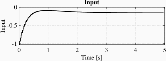
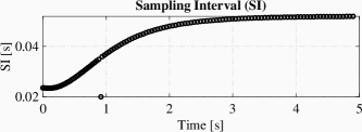
Figure 1: The state trajectory, input profile and sampling interval of event-triggered adaptive control in Example VI.1.

 

Example VI.2

(Event-triggered Stabilization with Dynamic Gain) Consider the following nonlinear system

$$\dot{z} = -z+w_{3}x$$

$$\dot{x} = w_{1}z\sin x+w_{2}x+bu$$

where $w_{1}$, $w_{2}$ and $w_{3}$ are unknown parameters and $0<b<1$. Note that when $V(z)=z^{2}$, one has $\dot{V}(z)\leq-z^{2}+px^{2}$ for any unknown constant $p\geq w_{3}^{2}$ and thus Assumption V.3 is satisfied. And $|w_{1}z\sin x+w_{2}x|\leq c(|z|+|x|)$ for some $c\geq\max\{|w_{1}|,|w_{2}|\}$, that is, inequality (48) is verified for $m_{1}=1$ and $m_{2}=1$. Then, we propose the sampling controller as in (49) and the closed-loop system is written as

$$\dot{z} = -z+w_{3}x$$

$$\dot{x} = w_{1}z\sin x+w_{2}x-b\hat{\theta}\rho(x)x+b\varpi,$$

$$\dot{\hat{\theta}} = \lambda\rho(x)x^{2},\;\lambda>0$$

where $\varpi(t)=-\hat{\theta}(t_{k})\rho(x(t_{k}))x(t_{k})+\hat{\theta}(t)\rho(x(t))x(t)$ is the sampling error. Let $V(\Xi)=\frac{1}{2}x^{2}+\frac{1}{2}b\lambda^{-1}\tilde{\theta}^{2}+2z^{2}$ and $\dot{V}(z,x,\tilde{\theta})\leq-|z|^{2}+\left(c^{2}/4+c+b^{2}q/4+2p-b\theta\rho(x)\right)x^{2}+\varpi^{2}/q.$ Select $\rho(x)=1$ and $\theta\geq\left(c^{2}/4+c+2p\right)/b+bq/4.$ Then, $\dot{V}(z,x,\tilde{\theta})\leq-\|\xi\|^{2}+\varpi^{2}/q$. Note that $\dot{\varpi}=-\dot{\hat{\theta}}x-2\hat{\theta}\dot{x}$ and let $U(\varpi)=\frac{1}{2}\varpi^{2}$. The inequality (57) is satisfied, i.e., $\dot{U}(\varpi)\leq\bar{\alpha}_{\beta}\bar{\sigma}(\xi)\|\xi\|^{2}+\alpha(\hat{\theta})\varpi^{2}$ where

$$\alpha(\hat{\theta})=1+\hat{\theta}^{2}+\hat{\theta}^{4}+2\bar{b}|\hat{\theta}|$$

$$\bar{\alpha}_{\beta}=\max\{\lambda^{2}/4,c^{2}+b^{2}\}$$

$$\bar{\sigma}(\xi)=1+\|\xi\|^{4}.$$

Note that $\frac{1}{2}x^{2}+\frac{1}{2}\lambda^{-1}\tilde{\theta}^{2}+2z^{2}\leq\bar{V}(z,x,\tilde{\theta})=(1+1/b)V(z,x,\tilde{\theta})\leq s\left[\frac{1}{2}x^{2}+\frac{1}{2}\lambda^{-1}\tilde{\theta}^{2}+2z^{2}\right]$ where $s\geq\max\{1+1/b,1+b\}$. Let $\hat{k}=\max\{2\bar{\alpha}_{\beta},1\}$ and $\Delta(\xi)=\bar{\sigma}(\xi)+1$. Let $\rho(\chi)=4+2\chi^{2}/\underline{\iota}^{2}$ and $V_{\Xi}(\Xi)=\int_{{}_{0}}^{\bar{V}(z,x,\tilde{\theta})}\hat{k}\rho(\tau)d\tau$. Let $\bar{\iota}=\max\{\frac{1}{2}\lambda^{-1},2\}$ and $\underline{\iota}=\frac{1}{2}\min\{\lambda^{-1},1\}$. The derivative of $V_{\Xi}(\Xi)$ becomes

$$\dot{V}_{\Xi}(\Xi)\leq-\hat{k}\Delta(\xi)\|\xi\|^{2}+\frac{64\hat{k}s^{2}\bar{\iota}^{2}}{\underline{\iota}^{2}q}\left(|\theta|^{4}+1\right)$$

$$\times\left(\left(|\hat{\theta}|+|\varpi|\sqrt{2/q}\right)^{4}+1\right)$$

Let

$$q\geq\bar{c}\max\left\{2,\frac{64\hat{k}s^{2}\bar{\iota}^{2}}{\underline{\iota}^{2}}\left(|\theta|^{4}+1\right)\right\}.$$

Then, inequality (59) is satisfied with $\bar{\varkappa}(\hat{\theta},\varpi)=\frac{\left(|\hat{\theta}|+|\varpi|\right)^{4}+1}{\bar{c}}$. Then, $\bar{\gamma}(\hat{\theta},\varpi)=\bar{\varkappa}(\hat{\theta},\varpi)/2+\bar{\alpha}(\hat{\theta})+\frac{1}{2}$ where $\alpha(\hat{\theta})=1+\hat{\theta}^{2}+\hat{\theta}^{4}+2\bar{b}|\hat{\theta}|$. Finally, the event-triggered law is designed according to Theorem V.2, as follows,

$$t_{k+1}=\inf_{t\geq t_{k}}\{(t-t_{k})\max_{\tau\in[t_{k},t]}\{\bar{\gamma}(\hat{\theta}(\tau),\varpi(\tau))\varpi^{2}(\tau)\}$$

$$\geq\frac{1}{4}\|\varpi_{[t_{k},t]}\|^{2},\;\text{and }\|\varpi_{[t_{k},t]}\|\neq 0\}.$$

The simulation result is illustrated in Fig 2, which includes figures of state trajectories, input signal and sampling intervals showing that the system trajectories converge to the origin without Zeno behavior.

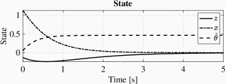
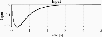
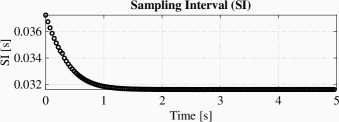
Figure 2: The state trajectory, input profile and sampling interval of event-triggered adaptive control in Example VI.2.

 

VII Conclusion

In this paper, we propose a novel sampling control framework based on the emulation technique where the sampling error is regarded as the auxiliary input to the emulated system. The design of periodic sampling and event-triggered control law utilizes the supremum norm of sampling error and renders the error dynamics bounded-input-bounded-state (BIBS), when coupled with system dynamics, achieves global or semi-global stabilization. The proposed framework is then extended to tackle the event-triggered and periodic sampling stabilization for systems with dynamic uncertainties. The proposed framework is further extended to solve two classes of event-triggered universal adaptive control problems. It would be very interesting to consider the case where the adaptation dynamics is also sampled and periodic event-triggered control along this research line.

Lemma .1

(Parameterized Changing Supply Functions, Lemma 6.1 in [6]) Consider the system $\dot{\xi}=f(\xi,\varpi)$ with $\xi=\text{col}(z,x)\in\mathbb{R}^{n}$ and $\varpi\in\mathbb{R}^{m}$. Suppose there exists a supplying function $V(\xi)$ satisfying

$$\underline{\alpha}(\|\xi\|)\leq V(\xi)\leq\bar{\alpha}(\|\xi\|,s)$$

$$\dot{V}(x)\leq-\alpha(\|x\|)+p\sigma(\|\varpi\|)$$

for $\mathcal{K}_{\infty}$ functions $\alpha$, $\underline{\alpha}$, $\sigma$, a parameterized $\mathcal{K}_{\infty}$ function $\bar{\alpha}$, and positive number $p$ and $s$. Then, for any smooth function $\Delta:\mathbb{R}^{n}\rightarrow[0,\infty)$ and positive number $k$, there exists a continuously differentiable function $V^{\prime}(\xi)$ satisfying

$$\underline{\alpha}^{\prime}(\|\xi\|)\leq V^{\prime}(\xi)\leq\bar{\alpha}^{\prime}(\|\xi\|,s^{\prime})$$

$$\dot{V}^{\prime}(x)\leq-k\Delta(\xi)\alpha(\|x\|)+p^{\prime}\varkappa(z,\varpi)\sigma(\|\varpi\|)$$

for a $\mathcal{K}_{\infty}$ functions $\underline{\alpha}^{\prime}$, a parameterized $\mathcal{K}_{\infty}$ function $\bar{\alpha}^{\prime}$, a $\mathcal{SN}$ function $\varkappa$ and positive numbers $p^{\prime}$ and $s^{\prime}$. Moreover, if the functions $\alpha$, $\underline{\alpha},$ $\bar{\alpha}$, $\sigma$ and $\Delta$ are known, so are the functions $\alpha^{\prime}$, $\bar{\alpha}^{\prime}$ and $\varkappa$. The positive numbers $s$, $p$, $k$, $s^{\prime}$ and $p^{\prime}$ are not necessarily known.  

Proof of Theorem III.2: It suffices to show condition (23) imply (22) and meanwhile it is guaranteed that the boundedness of signals $\varpi$, i.e., $\|\varpi(t)\|\leq R_{0}$, $\forall t\geq t_{0}$. From (23), one has $\omega\underline{\alpha}_{\varpi}(s)-2\gamma(s)>0,\;\forall 0<s<R_{0}$. Since $\underline{\alpha}_{\varpi}$ and $\gamma$ are continuous functions, there exists a sufficiently small $\tilde{R}$ such that

$$\omega\underline{\alpha}_{\varpi}(R_{0}+s)-2\gamma(R_{0}+s)>0,\;\forall 0\leq s\leq\tilde{R},$$

It, together with (23), further implies

$$2\gamma(s)<\omega\underline{\alpha}_{\varpi}(s),\;\forall 0<s\leq R_{0}+\tilde{R}.$$ (60)

We will prove that $\|\varpi(t)\|\leq R_{0},\;\forall t\geq t_{0}$. If this is not true, there exists a finite time $t_{a}>t_{0}$ such that $\|\varpi(t)\|\leq R_{0}+\tilde{R},\;\forall t\in[t_{0},t_{a}]$ but $\|\varpi(t_{a})\|>R_{0}$. Due to (60) and the periodic sampling law in (21), one have

$$2(t-t_{i})\gamma(\|\varpi\|_{[t_{i},t]})\leq 2T\gamma(\|\varpi\|_{[t_{i},t]})<\underline{\alpha}_{\varpi}(\|\varpi\|_{[t_{i},t]})$$

$$\leq\max_{\tau\in[t_{i},t]}\{U(\varpi(\tau))\},\;\forall t\in[t_{i},t_{i}+T),$$

$$\forall t_{i}=\{t_{0},t_{0}+T,\cdots,t_{0}+(\bar{k}+1)T\},$$ (61)

where $\bar{k}=\max_{k}\left\{k\mid t_{0}+(k+1)T\leq t_{a}\right\}$. Therefore, (22) is valid for $t<t_{a}$ and $T\leq\bar{t}_{k+1}-t_{k}$, $\forall k\in\mathbb{N}$ where $\bar{t}_{k+1}$ is given in (20). By Remark III.4, results of Theorem III.1 hold, and one has $V_{q}(x(t))\leq V_{q}(x(t_{0}))$. Due to $x(t_{0})\in\mathcal{X}$, one has $V_{q}(x(t))\leq V_{q}(x(t_{0}))\leq\underline{\alpha}_{q}\circ\sigma_{\varpi}^{-1}\circ\alpha_{\varpi}(R_{0})$, that is $\mathcal{S}\subseteq\mathbb{R}^{n}$ is a positively invariant set. By Remark III.1, one has $\|\varpi(t)\|\leq R_{0},\forall t_{0}\leq t\leq t_{a}$ which causes a contradiction to $\|\varpi(t_{a})\|>R_{0}$. Therefore, $\|\varpi(t)\|\leq R_{0},\;\forall t\geq t_{0}$. As a result, conducting similar analysis as above for $t\geq t_{0}$ shows that (22) is valid for $t\geq t_{0}$ and using the discussion in Remark III.4 completes the proof.  

Proof of Corollary III.1: The fact that $\sigma_{\varpi}(s)=\mathcal{O}(\alpha(s))$ as $s\rightarrow 0^{+}$ implies it is always possible to find a new supply function $V_{q}(x)\sim\{\underline{\alpha}_{q},\bar{\alpha}_{q},\alpha_{q},(\sigma_{q},\varsigma_{q})\mid\dot{x}=f_{c}(x,\varpi,d)\}$ for some $\mathcal{K}_{\infty}$ functions $\underline{\alpha}_{q}$, $\bar{\alpha}_{q}$, $\sigma_{q}$ and $\varsigma_{q}$, that can be calculated accordingly. Denote $\upsilon=\text{col}(x,w)$. Following the first proof step of Theorem III.1, one has

$$U(\varpi(t))\leq-2\int_{t_{k}^{+}}^{t}\hat{\alpha}_{\varpi}(\|\varpi(\tau)\|)d\tau+2\int_{t_{k}^{+}}^{t}\sigma_{\varpi}(\|x(\tau)\|)d\tau$$

$$+2\int_{t_{k}^{+}}^{t}\varsigma_{\varpi}(\|d(\tau)\|)d\tau,\;\forall t\in[t_{k},t_{k+1}].$$

Let $\bar{V}(x,\varpi)=V_{q}(x)+U(\varpi)$ be the Lyapunov function candidate. Similarly, one has

$$\bar{V}(x(t),\varpi(t))-\bar{V}(x(t_{k}^{+}),\varpi(t_{k}^{+}))\leq-\int_{t_{k}^{+}}^{t}\alpha_{\gamma}(\|x(\tau)\|)d\tau$$

$$-\int_{t_{k}^{+}}^{t}\gamma_{\alpha}(\|\varpi(\tau)\|)d\tau+\int_{t_{k}^{+}}^{t}\varsigma_{\upsilon}(\|d(\tau)\|)d\tau$$

$$\leq-\int_{t_{k}^{+}}^{t}\alpha_{\upsilon}(\|\upsilon(\tau)\|)d\tau+\int_{t_{k}^{+}}^{t}\varsigma_{\upsilon}(\|d(\tau)\|)d\tau,\;\forall t\in[t_{k},t_{k+1}],$$

where functions $\alpha_{\upsilon}$ is selected as $\alpha_{\upsilon}(\|\upsilon\|)\leq\alpha_{\gamma}(\|x\|)+\gamma_{\alpha}(\|\varpi\|)$ and $\varsigma_{\upsilon}(s)\geq 2\varsigma_{\varpi}(s)+\varsigma_{q}(s)$. Note that there exist functions $\underline{\alpha}_{\upsilon}$ and $\bar{\alpha}_{\upsilon}$ satisfying

$$\underline{\alpha}_{\upsilon}(\|\upsilon\|)\leq\underline{\alpha}_{q}(\|x\|)+\underline{\alpha}_{\varpi}(\|\varpi\|),$$

$$\bar{\alpha}_{\upsilon}(\|\upsilon\|)\leq\bar{\alpha}_{q}(\|x\|)+\bar{\alpha}_{\varpi}(\|\varpi\|),$$

such that $\underline{\alpha}_{\upsilon}(\|\upsilon\|)\leq\bar{V}(x,\varpi)\leq\bar{\alpha}_{\upsilon}(\|\upsilon\|)$. As a result, $\bar{V}(t)-\bar{V}(t_{k})\leq-\int_{t_{k}^{+}}^{t}\alpha_{\upsilon}\circ\bar{\alpha}_{\upsilon}^{-1}(\bar{V}(\tau))d\tau+\int_{t_{k}^{+}}^{t}\varsigma_{\upsilon}(\|d(\tau)\|)d\tau$ which implies that any trajectory starting outside $B$ will eventually goes inside $B$ where $B:=\{\upsilon\mid\bar{V}\leq\bar{\alpha}_{\upsilon}\circ\alpha_{\upsilon}{}^{-1}\circ\varsigma_{\upsilon}(\bar{d})\}$. and $\|x\|\leq\underline{\alpha}_{\upsilon}^{-1}\circ\bar{\alpha}_{\upsilon}\circ\alpha_{\upsilon}{}^{-1}\circ\varsigma_{\upsilon}(\bar{d})$ is satisfied. Similar to the proof of Theorem III.1, Zeno-freeness depends on the condition $\gamma(s)=\mathcal{O}(\underline{\alpha}_{\varpi}(s))$ as $s\rightarrow 0^{+}$ and can be proved in the same way.

References

• [1] A. Anta and P. Tabuada. To sample or not to sample: Self-triggered control for nonlinear systems. IEEE Transactions on Automatic Control, 55(9):2030–2042, 2010.
• [2] M. Araki. Recent developments in digital control theory. IFAC Proceedings Volumes, 26(2):951–960, 1993.
• [3] T. Chen and B. A. Francis. Optimal sampled-data control systems. Springer Science & Business Media, 2012.
• [4] Z. Chen and H. Fujioka. Performance analysis of nonlinear sampled-data emulated controllers. IEEE Transactions on Automatic Control, 59(10):2778–2783, 2014.
• [5] Z. Chen, Q.-L. Han, Y. Yan, and Z.-G. Wu. How often should one update control and estimation: review of networked triggering techniques. Science China Information Sciences, 63:150201:1–18, 2020.
• [6] Z. Chen and J. Huang. Stabilization and Regulation of Nonlinear Systems. Springer International Publishing, 2015.
• [7] C. De Persis, R. Sailer, and F. Wirth. On a small-gain approach to distributed event-triggered control. IFAC Proceedings Volumes, 44(1):2401–2406, 2011.
• [8] V. S. Dolk, D. P. Borgers, and W. P. M. H. Heemels. Output-based and decentralized dynamic event-triggered control with guaranteed $\mathcal{L}_{p}$- gain performance and zeno-freeness. IEEE Transactions on Automatic Control, 62(1):34–49, 2017.
• [9] Y. Fan, G. Feng, Y. Wang, and C. Song. Distributed event-triggered control of multi-agent systems with combinational measurements. Automatica, 49(2):671–675, 2013.
• [10] E. Fridman, M. Dambrineb, and N. Yeganefar. On input-to-state stability of systems with time-delay: A matrix inequalities approach. Automatica, 44:2364–2369, 2008.
• [11] E. Fridman, A. Seuret, and J.P. Richard. Robust sampled-data stabilization of linear systems: an input delay approach. Automatica, 40(8):1441–1446, 2004.
• [12] E. Fridman, R. Shaked, and V. Suplin. Input/output delay approach to robust sampled-data h-infty control. Systems & Control Letters, 54(3):271–282, 2005.
• [13] J. Huang, W. Wang, C. Wen, and G. Li. Adaptive event-triggered control of nonlinear systems with controller and parameter estimator triggering. IEEE Transactions on Automatic Control, 65(1):318–324, 2019.
• [14] I. Karafyllis and C. Kravaris. Global stability results for systems under sampled-data control. International Journal of Robust and Nonlinear Control, 19(10):1105–1128, 2009.
• [15] G. D. Khan, Z. Chen, and L. Zhu. A new approach for event-triggered stabilization and output regulation of nonlinear systems. IEEE Transactions on Automatic Control, 65(8):3592–3599, 2020.
• [16] D. Liberzon, D. Nešić, and A. R. Teel. Lyapunov-based small-gain theorems for hybrid systems. IEEE Transactions on Automatic control, 59(6):1395–1410, 2014.
• [17] T. Liu and Z. P. Jiang. Event-based control of nonlinear systems with partial state and output feedback. Automatica, 53:10–22, 2015.
• [18] T. Liu and Z. P. Jiang. A small-gain approach to robust event-triggered control of nonlinear systems. IEEE Transactions on Automatic Control, 60(8):2072–2085, 2015.
• [19] N. Marchand, S. Durand, and J. F. G. Castellanos. A general formula for event-based stabilization of nonlinear systems. IEEE Transactions on Automatic Control, 58(5):1332–1337, 2013.
• [20] M. Mazo, A. Anta, and P. Tabuada. An ISS self-triggered implementation of linear controllers. Automatica, 46(8):1310–1314, 2010.
• [21] R. Moheimani. Perspectives in robust control, volume 268. Springer Science & Business Media, 2001.
• [22] D. Nesic, A. R. Teel, and D. Carnevale. Explicit computation of the sampling period in emulation of controllers for nonlinear sampled-data systems. IEEE Transactions on Automatic Control, 54(3):619–624, 2009.
• [23] G. S. Seyboth, D. V. Dimarogonas, and K. H. Johansson. Event-based broadcasting for multi-agent average consensus. Automatica, 49(1):245–252, 2013.
• [24] E. Sontag and A. Teel. Changing supply function in input/state stable systems. IEEE Transactions on Automatic Control, 40:1476–1478, 1995.
• [25] P. Tabuada. Event-triggered real-time scheduling of stabilizing control tasks. IEEE Transactions on Automatic Control, 52(9):1680–1685, 2007.
• [26] P. Tallapragada and N. Chopra. On event triggered tracking for nonlinear systems. IEEE Transactions on Automatic Control, 58(9):2343–2348, 2013.
• [27] C. Wang, C. Wen, and Q. Hu. Event-triggered adaptive control for a class of nonlinear systems with unknown control direction and sensor faults. IEEE Transactions on Automatic Control, 65(2):763–770, 2019.
• [28] L. Xing, C. Wen, Z. Liu, H. Su, and J. Cai. Event-triggered adaptive control for a class of uncertain nonlinear systems. IEEE Transactions on Automatic Control, 62(4):2071–2076, 2016.
• [29] X. Yi, K. Liu, D.V. Dimarogonas, and K. H. Johansson. Dynamic event-triggered and self-triggered control for multi-agent systems. IEEE Transactions on Automatic Control, 64(8):3300–3307, 2018.
• [30] L. Zhu, Z. Chen, D.J. Hill, and S. Du. Event-triggered controllers based on the supremum norm of sampling-induced error. Automatica, 128:109532, 2021.