Emergent SU(2)₁ conformal symmetry in the spin-1/2 Kitaev-Gamma chain with a Dzyaloshinskii-Moriya interaction

Abstract

We study the one-dimensional spin-1/2 Kitaev-Gamma model with a bond-dependent Dzyaloshinskii-Moriya (DM) interaction, which can be induced by an electric field applied in the third direction where the first and second directions refer to the two bond directions in the model. By a combination of field theory and symmetry analysis, an extended gapless phase with an emergent SU(2)₁ conformal symmetry is found in the phase diagram of the spin-1/2 Kitaev-Gamma-DM chain. The analytic predictions are in good agreements with numerical results obtained from density matrix renormalization group simulations.

I Introduction

As potential realizations of the Kitaev spin-1/2 model on the two-dimensional (2D) honeycomb lattice Kitaev2006 ; Nayak2008 , Kitaev materials (including A₂IrO₃ (A$=$Li, Na), $\alpha$-RuCl₃, etc.) have attracted intensive research attentions in the past decade Jackeli2009 ; Chaloupka2010 ; Singh2010 ; Price2012 ; Singh2012 ; Plumb2014 ; Kim2015 ; Winter2016 ; Baek2017 ; Leahy2017 ; Sears2017 ; Wolter2017 ; Zheng2017 ; Rousochatzakis2017 ; Kasahara2018 ; Rau2014 ; Ran2017 ; Wang2017 ; Catuneanu2018 ; Gohlke2018 ; Liu2011 ; Chaloupka2013 ; Johnson2015 ; Motome2020 . Motivated by the theoretical difficulties in strongly correlated systems in 2D, there has been a surge of research interests in studying 1D generalized Kitaev spin models Sela2014 ; Agrapidis2018 ; Agrapidis2019 ; Catuneanu2019 ; Yang2020 ; Yang2020a ; Yang2020b ; Yang2021b ; Yang2022 ; Yang2022b ; Yang2020c ; Luo2021 ; Luo2021b ; You2020 ; Sorensen2021 , which can be constructed by selecting one or several rows out of the honeycomb lattice. The hope is that such 1D studies can help understand the 2D Kitaev physics, and indeed, it has been shown that the 2D zigzag order in the Kitaev-Heisenberg-Gamma model can be obtained by weakly coupling an infinite number of 1D chains Yang2022b .

Besides providing hints for 2D physics, the 1D Kitaev spin models are also intriguing on their own, containing exotic strongly correlated physics. For example, in the 1D spin-1/2 Kitaev-Gamma model, it has been found that about 67% of the entire phase diagram is occupied by a gapless phase whose low energy physics can be described by an emergent SU(2)₁ Wess-Zumino-Witten (WZW) model, which is intimately related to the intricate discrete nonsymmorphic symmetry group of the system Yang2020 . In addition to the emergent SU(2)₁ phase, the spin-1/2 Kitaev-Gamma chain also contains two magnetically ordered phases with symmetry breaking patterns $O_{h}\rightarrow D_{4}$ Yang2020 and $O_{h}\rightarrow D_{3}$ Yang2021b , as well as another gapless phase with central charge $c=1/2$ located in the vicinity of the antiferromagnetic (AFM) Kitaev point Luo2021 , where $O_{h}$ is the full octahedral group and $D_{n}$ is the dihedral group of order $2n$, showcasing rich strongly correlated physics in such systems.

On the other hand, nearest neighbor Dzyaloshinskii-Moriya (DM) interactions Dzyaloshinskii1957 ; Dzyaloshinskii1964 ; Moriya1960 ; Fert1980 ; Fert1990 are ubiquitous in quantum magnetic systems which break the spatial inversion symmetry and can lead to exotic magnetic textures such as skyrmions Heinze2011 ; Yu2010 ; Bogdanov1994 ; Rolber2006 and chiral magnetic orders Dzyaloshinskii1965 ; Bogdanov1989 . In Kitaev materials, the DM interactions can be conveniently induced and manipulated by external electric fields, which have been studied under the context of the electromagnetic controls of Kitaev materials Furuya2021 ; Chari2021 . It is noteworthy to mention that the DM interactions in Kitaev materials exhibit a nonuniform bond-dependent structure.

In this work, we study the effects of a DM interaction in the 1D spin-1/2 Kitaev-Gamma model, which can be created by applying an electric field along the third direction (where the first and second directions refer to the two bond directions in the 1D model, see Fig. 1 (a) for details). Since in real Kitaev materials, the Kitaev and Gamma interactions usually dominate over other interactions such as the Heisenberg and $\Gamma^{\prime}$ terms, our work provides a perturbative starting point for the analysis of more complicated interactions as well as an extrapolation to 2D in the presence of a DM interaction.

We start from a pure Kitaev spin-1/2 chain with a DM interaction. The first important result of our work is that there is a two-site periodic unitary transformation $V_{2}$, which maps the 1D Kitaev-DM model to the Kitaev-Gamma model and vice versa. Using the known phase diagram of the 1D spin-1/2 Kitaev-Gamma model, the effects of the DM interaction on the spin-1/2 Kitaev chain is thereby fully understood.

We then proceed to studying the 1D Kitaev-Gamma-DM model. The strategy is to take the emergent SU(2)₁ phase in the Kitaev-Gamma chain as the unperturbed system, and treat the DM interaction as a perturbation. Remarkably, although there is a dimension $3/2$ operator in the low energy conformal field theory (CFT), such operator is a total derivative and vanishes if periodic boundary condition is imposed. Therefore, even with a nonzero DM interaction, the system remains to have an emergent SU(2)₁ conformal symmetry in an extended region in the phase diagram. The theoretical predictions from perturbation theory are in excellent agreements with our density matrix renormalization group (DMRG) numerical simulations.

Two observations are in order. First, the aforementioned unitary transformation $V_{2}$ is a duality transformation which maps the Kitaev-Gamma-DM model to itself with a different set of parameters, thereby enlarging the region occupied by the emergent SU(2)₁ phase in the phase diagram. Second, it is interesting to compare the symmetry groups of the Kitaev-Gamma and Kitaev-Gamma-DM models. The symmetry analysis is facilitated by a six-sublattice rotation $U_{6}$ Yang2020 which hold for both models. In the $U_{6}$ frame, it has been shown in Ref. Yang2020, that the symmetry group $G$ of the Kitaev-Gamma model satisfies $G/\mathopen{<}T_{3a}\mathclose{>}\cong O_{h}$ where $T_{na}$ represents the translation operator by $n$ sites. On the other hand, the symmetry group $G_{z}$ of the Kitaev-Gamma-DM model is found to satisfy $G_{z}/\mathopen{<}T_{6a}\mathclose{>}\cong O_{h}$. Hence, the symmetry group in the Kitaev-Gamma-DM model is “halved” compared with the Kitaev-Gamma model. Notice that the unit cell of the spin-1/2 Kitaev-Gamma-DM model contains an even number of sites, which naively corresponds to an integer spin. Hence it is rather an unexpected result that such “integer” spin system displays an emergent gapless phase at low energies, which of course essentially originates from the intricate nonsymmorphic group structure.

The rest of the paper is organized as follows. Sec. II introduces the model Hamiltonian and discusses the unitarily equivalent relations in the model. In Sec. III, the emergent SU(2)₁ conformal symmetry is obtained by treating the DM interaction as a perturbation on the known SU(2)₁ phase in the Kitaev-Gamma model. Sec. IV presents a symmetry analysis, which proves that the analysis in Sec. III has exhausted all possible relevant and marginal operators in the low energy field theory. Sec. V shows the numerical evidence for the emergent SU(2)₁ conformal symmetry. Finally in Sec. VI, we summarize the main results of this work.

II The model

II.1 Model Hamiltonian

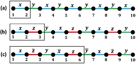
Figure 1: Bond patterns of the Kitaev-Gamma chain (a) without sublattice rotation, (b) after the six-sublattice rotation, (c) with a nonzero DM interaction after six-sublattice rotation. The black squares represent the unit cells.

The Hamiltonian of the spin-1/2 Kitaev-Gamma chain is defined as

$$H=\sum_{\langle ij\rangle\in\gamma\,\text{bond}}\big{[}KS_{i}^{\gamma}S_{j}^{\gamma}+\Gamma(S_{i}^{\alpha}S_{j}^{\beta}+S_{i}^{\beta}S_{j}^{\alpha})\big{]},$$ (1)

in which $(\alpha,\beta,\gamma)$ form a right-handed coordinate system; the pattern for the bond $\gamma$ is shown in Fig. 1 (a); and the couplings $K$ and $\Gamma$ can be parametrized as $K=\cos(\psi)$, $\Gamma=\sin(\psi)$. Since the global spin rotation around $z$-axis by an angle $\pi$ (denoted as $R(\hat{z},\pi)$) changes the sign of $\Gamma$, it is enough to consider $\Gamma>0$, i.e., $\psi\in[0,\pi]$. As shown by Ref. Yang2020, , the system has an emergent SU(2)₁ conformal symmetry at low energies for $\theta\in[\psi_{c},\pi]$ where $\psi_{c}\sim 0.33\pi$.

In Kitaev materials, nearest neighbor DM interactions can be induced by applying electric fields. Let $\gamma$ be the bond connecting nearest neighboring sites $i$ and $j$, and consider the right-handed coordinate system $(\gamma,\alpha,\beta)$. An electric field is called in-plane if its direction is within the $\alpha\beta$-plane, and out-of-plane if it is parallel with the $\gamma$-axis. As discussed in Ref. Furuya2021, , an in-plane electric field induces a DM interaction of the form

$$D_{M}(S_{i}^{\alpha}S_{i+1}^{\beta}-S_{i}^{\beta}S_{i+1}^{\alpha}).$$ (2)

In this work, we consider the type of DM interaction which can be induced by an electric field along the $z$-direction. As can be seen from Fig. 1 (a), an electric field along z-direction corresponds to an in-plane electric field for every bond in the chain. Adding Eq. (2) to Eq. (1), the Hamiltonian becomes

$$H_{z}=\sum_{\langle ij\rangle\in\gamma\,\text{bond}}\big{[}KS_{i}^{\gamma}S_{j}^{\gamma}+\Gamma_{1}S_{i}^{\alpha}S_{j}^{\beta}+\Gamma_{2}S_{i}^{\beta}S_{j}^{\alpha}\big{]},$$ (3)

in which

$$\Gamma_{1}=\Gamma+D_{M},\leavevmode\nobreak\ \Gamma_{2}=\Gamma-D_{M};$$ (4)

the bond pattern for $\gamma$ is shown in Fig. 1 (a); and $(\gamma\alpha\beta)$ form a right-handed coordinate system. More explicitly, the form of the Hamiltonian within a two-site unit cell of sites $\{1,2\}$ is given by

$$H_{z,12} = KS^{x}_{1}S^{x}_{2}+\Gamma_{1}S^{y}_{1}S^{z}_{2}+\Gamma_{2}S^{z}_{1}S^{y}_{2},$$

$$H_{z,23} = KS^{y}_{2}S^{y}_{3}+\Gamma_{1}S^{z}_{2}S^{x}_{3}+\Gamma_{2}S^{x}_{2}S^{z}_{3}.$$ (5)

Finally, a useful parametrization is

$$K = \cos(\theta),$$

$$D_{M} = \sin(\theta)\cos(\phi),$$

$$\Gamma = \sin(\theta)\sin(\phi),$$ (6)

in which $\theta\in(0,\pi)$, $\phi\in(0,2\pi)$. Hence, the full parameter space of the model is a unit sphere.

II.2 Six-sublattice rotation

A useful unitary transformation is the six-sublattice rotation $U_{6}$, defined as

$$\text{Sublattice $1$}: (x,y,z) \rightarrow(x^{\prime},y^{\prime},z^{\prime}),$$

$$\text{Sublattice $2$}: (x,y,z) \rightarrow(-x^{\prime},-z^{\prime},-y^{\prime}),$$

$$\text{Sublattice $3$}: (x,y,z) \rightarrow(y^{\prime},z^{\prime},x^{\prime}),$$

$$\text{Sublattice $4$}: (x,y,z) \rightarrow(-y^{\prime},-x^{\prime},-z^{\prime}),$$

$$\text{Sublattice $5$}: (x,y,z) \rightarrow(z^{\prime},x^{\prime},y^{\prime}),$$

$$\text{Sublattice $6$}: (x,y,z) \rightarrow(-z^{\prime},-y^{\prime},-x^{\prime}),$$ (7)

in which “Sublattice $i$” ($1\leq i\leq 6$) represents all the sites $i+6n$ ($n\in\mathbb{Z}$) in the chain, and we have abbreviated $S^{\alpha}$ ($S^{\prime\alpha}$) as $\alpha$ ($\alpha^{\prime}$) for short ($\alpha=x,y,z$).

In the six-sublattice rotated frame, the Hamiltonian is

$$H^{\prime}_{z}=\sum_{\langle ij\rangle\in\gamma\,\text{bond}}\big{[}-KS_{i}^{\gamma}S_{j}^{\gamma}-\Gamma_{1}S_{i}^{\alpha}S_{j}^{\alpha}-\Gamma_{2}S_{i}^{\beta}S_{j}^{\beta}\big{]},$$ (8)

in which $\gamma\in\{x,\bar{z},y,\bar{x},z,\bar{y}\}$ has a six-site periodicity as shown in Fig. 1 (c); $S_{j}^{\gamma}=S_{j}^{\bar{\gamma}}$; $(\gamma\alpha\beta)$ form a right-handed coordinate system for $\gamma\in\{x,y,z\}$, and they form a left-handed system when $\gamma\in\{\bar{x},\bar{y},\bar{z}\}$. More explicitly, the form of the Hamiltonian within a six-site unit cell of sites $\{1,2,3,4,5,6\}$ is

$$H^{\prime}_{z,12} = -KS^{x}_{1}S^{x}_{2}-\Gamma_{1}S^{y}_{1}S^{y}_{2}-\Gamma_{2}S^{z}_{1}S^{z}_{2},$$

$$H^{\prime}_{z,23} = -KS^{z}_{2}S^{z}_{3}-\Gamma_{1}S^{y}_{2}S^{y}_{3}-\Gamma_{2}S^{x}_{2}S^{x}_{3},$$

$$H^{\prime}_{z,34} = -KS^{y}_{3}S^{y}_{4}-\Gamma_{1}S^{z}_{3}S^{z}_{4}-\Gamma_{2}S^{x}_{3}S^{x}_{4},$$

$$H^{\prime}_{z,45} = -KS^{x}_{4}S^{x}_{5}-\Gamma_{1}S^{z}_{4}S^{z}_{5}-\Gamma_{2}S^{y}_{4}S^{y}_{5},$$

$$H^{\prime}_{z,56} = -KS^{z}_{5}S^{z}_{6}-\Gamma_{1}S^{x}_{5}S^{x}_{6}-\Gamma_{2}S^{y}_{5}S^{y}_{6},$$

$$H^{\prime}_{z,67} = -KS^{y}_{6}S^{y}_{7}-\Gamma_{1}S^{x}_{6}S^{x}_{7}-\Gamma_{2}S^{z}_{6}S^{z}_{7}.$$ (9)

Form here on, we stick to the six-sublattice rotated frame in this work unless otherwise stated.

II.3 Unitarily equivalent relations

Clearly, both $\Gamma_{1}$ and $\Gamma_{2}$ change sign under $R(\hat{z},\pi)$ within the original frame (i.e., without six-sublattice rotation $U_{6}$). Hence there is the equivalence

$$(K,\Gamma,D_{M})\simeq(K,-\Gamma,-D_{M}).$$ (10)

Because of Eq. (10), it is enough to consider the $\Gamma>0$ region.

In addition, consider a two-sublattice rotation $V_{2}$ which acts on odd sites as a spin rotation $R(\hat{z},\pi)$ but leaves all even sites unchanged. Straightforward calculations show that the Kitaev, Gamma and DM terms transform under $V_{2}$ as

$$KS_{i}^{\gamma}S_{j}^{\gamma} \rightarrow -KS_{i}^{\gamma}S_{j}^{\gamma},$$

$$\Gamma(S_{i}^{\alpha}S_{j}^{\beta}+S_{i}^{\beta}S_{j}^{\alpha}) \rightarrow -\Gamma(S_{i}^{\alpha}S_{j}^{\beta}-S_{i}^{\beta}S_{j}^{\alpha}),$$

$$D_{M}(S_{i}^{\alpha}S_{i+1}^{\beta}-S_{i}^{\beta}S_{i+1}^{\alpha}) \rightarrow -D_{M}(S_{i}^{\alpha}S_{i+1}^{\beta}+S_{i}^{\beta}S_{i+1}^{\alpha}),$$

which hold for every bond. Hence, we also have the following equivalence

$$(K,\Gamma,D_{M})\simeq(-K,-D_{M},-\Gamma).$$ (12)

In terms of $(\theta,\phi)$ in Eq. (6), the equivalences in Eqs. (10,12) can be expressed as $(\theta,\phi)\simeq(\theta,-\phi)\simeq(\pi-\theta,\frac{3\pi}{2}-\phi)$. Therefore, it is enough to consider the region $\theta\in(0,\frac{\pi}{2})$, $\phi\in(0,\pi)$ in the phase diagram where $\theta$ and $\phi$ are defined in Eq. (6).

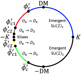
Figure 2: Phase diagram of the spin-1/2 Kitaev chain with DM interaction, where $K=\cos(\phi^{\prime})$, $D_{M}=\sin(\phi^{\prime})$.

Using Eq. (12), it can be seen that the Kitaev-DM model is mapped to the Kitaev-Gamma model. On the other hand, the phase diagram of the spin-1/2 Kitaev-Gamma chain has been studied in detail in Ref. Yang2020, and Ref. Yang2021b, . Therefore, we are able to directly obtain the phase diagram of the spin-1/2 Kitaev chain with a DM interaction as shown in Fig. 2, in which $K$ and $D_{M}$ are parametrized as

$$K=\cos(\phi^{\prime}),\leavevmode\nobreak\ D_{M}=\sin(\phi^{\prime}),$$ (13)

and the values of the phase transition points are $\phi^{\prime}_{c}=0.67\pi$, $\phi^{\prime}_{c1}=0.9\pi$, $\phi^{\prime}_{c2}=0.967\pi$, and $\bar{\phi^{\prime}}_{c}=2\pi-\phi^{\prime}_{c}$, $\bar{\phi}^{\prime}_{c1}=2\pi-\phi^{\prime}_{c1}$, $\bar{\phi}^{\prime}_{c2}=2\pi-\phi^{\prime}_{c2}$. Since $D_{M}$ changes sign under $R(\hat{z},\pi)$ whereas $K$ remains the same, it is enough to consider the region $\phi^{\prime}\in[0,\pi)$. For $\phi^{\prime}\in(0,\phi_{c})$, the system is in a gapless phase which has an emergent SU(2)₁ conformal symmetry at low energies; for $\phi^{\prime}\in(\phi^{\prime}_{c},\phi^{\prime}_{c1})$, the system is in an ordered phase with a spontaneous symmetry breaking pattern as $O_{h}\rightarrow D_{4}$; for $\phi^{\prime}\in(\phi^{\prime}_{c1},\phi^{\prime}_{c2})$, the system is in another ordered phase with a spontaneous symmetry breaking pattern as $O_{h}\rightarrow D_{3}$; for $\phi^{\prime}\in(\phi^{\prime}_{c2},\pi)$ named as “Kitaev” in Fig. 2, there is numerical evidence that the central charge in this region is $c=1/2$ Luo2021 .

III Emergent SU(2)₁ conformal symmetry in the spin-1/2 Kitaev-Gamma-DM chain

In this section, we study the spin-1/2 Kitaev-Gamma chain with a bond-dependent DM interaction, which can be induced by an electric field along $z$-direction.

Fig. 3 is a schematic plot of the front half of the unit sphere of the parameter space in terms of $\theta$ and $\phi$ as defined in Eq. (6). The back half of the sphere is not shown because of the equivalence in Eq. (10). We will analytically demonstrate that there is an emergent SU(2)₁ conformal symmetry at low energies in the “Emergent SU(2)₁ I” region in Fig. 3, which is analyzed by perturbing the Kitaev-Gamma model and treating the DM interaction as a perturbation. Then by using Eq. (10) and Eq. (12), we know that the regions marked with “Emergent SU(2)₁ II, III” also have an emergent SU(2)₁ conformal symmetry at low energies.

We emphasize that the phase diagram in Fig. 3 is only schematic. The phase boundaries of the three emergent SU(2)₁ regions are shown as dashed lines since their locations are not precisely determined. On the other hand, the phase transitions in the Kitaev-DM and Kitaev-Gamma models are known, which are shown as the red, brown and green cross symbols in Fig. 3, corresponding to $\phi^{\prime}_{c}$, $\phi^{\prime}_{c1}$ and $\phi^{\prime}_{c2}$ (or $\bar{\phi}^{\prime}_{c}$, $\bar{\phi}^{\prime}_{c1}$ and $\bar{\phi}^{\prime}_{c2}$) in Fig. 2, respectively.

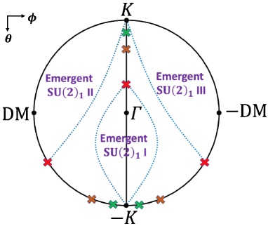
Figure 3: Schematic plot of the emergent SU(2)₁ phases in the phase diagram of the spin-1/2 Kitaev-Gamma chain with a DM interaction. The red, brown and green cross symbols correspond to the phase transitions at $\phi^{\prime}_{c}$, $\phi^{\prime}_{c1}$ and $\phi^{\prime}_{c2}$ (or $\bar{\phi}^{\prime}_{c}$, $\bar{\phi}^{\prime}_{c1}$ and $\bar{\phi}^{\prime}_{c2}$) in Fig. 2, respectively, in either the Kitaev-Gamma model or Kitaev-DM model.

III.1 Low energy field theory

In this subsection, treating the DM term as a perturbation, we derive the low energy field theory of the model. We will consider the $K<0$, $\Gamma<0$ region, which is in the back half of the sphere (not shown in Fig. 3). This region is equivalent with “Emergent SU(2)₁ I” phase in Fig. 3 according to Eq. (10).

III.1.1 Review of SU(2)₁ CFT for spin-1/2 Kitaev-Gamma chain

When $K=\Gamma_{1}=\Gamma_{2}<0$, the system in Eq. (8) reduces to the AFM Heisenberg model, which represents a hidden SU(2) symmetric point. It is known that at low energies, the spin-1/2 AFM Heisenberg model is described by the SU(2)₁ Wess-Zumino-Witten (WZW) model. The Hamiltonian density is of the Sugawara form

$$\mathcal{H}=\frac{2\pi}{3}v(\vec{J_{L}}\cdot\vec{J_{L}}+\vec{J_{R}}\cdot\vec{J_{R}})$$ (14)

with an additional marginally irrelevant term $-u\vec{J_{L}}\cdot\vec{J_{R}}$, in which $v$ is the spin velocity; $u>0$ is the coupling constant of the marginally irelevant term $\vec{J_{L}}\cdot\vec{J_{R}}$; and $\vec{J_{L}}$ and $\vec{J_{R}}$ defined by

$$\vec{J_{L}} = -\frac{1}{4\pi}\text{tr}[(\partial_{z}g)g^{\dagger}\vec{\sigma}]$$

$$\vec{J_{R}} = \frac{1}{4\pi}\text{tr}[g^{\dagger}(\partial_{\bar{z}}g)\vec{\sigma}],$$ (15)

are the left and right WZW currents, respectively, where the SU(2) matrix $g$ is the WZW primary field, $\sigma^{\alpha}$ ($\alpha=x,y,z$) are the three Pauli matrices, and $z=\tau+ix$ ($\bar{z}=\tau-ix$) is the holomorphic (anti-holomorphic) coordinate in the imaginary time formalism. This hidden SU(2) symmetric AFM point provides a starting point for a field theory perturbation for the regions nearby.

When $D_{M}=0$ but $K\neq\Gamma$, the system in Eq. (8) reduces to the Kitaev-Gamma model, and it has been shown in Ref. Yang2020, that the system is described by the SU(2)₁ WZW model at low energies. The spin operators are related to the SU(2)₁ low energy fields by the nonsymmorphic nonabelian bosonization formula:

$$\frac{1}{a}S_{i+3n}^{\alpha}=D^{\alpha}_{i}(J_{L}^{\alpha}+J_{R}^{\alpha})+C^{\alpha}_{i}\frac{1}{\sqrt{a}}(-)^{n}N^{\alpha},$$ (16)

in which $i=1,2,3$; $\alpha=x,y,z$; and

$$D_{1}^{z}=D_{2}^{y}=D_{3}^{x}(=D_{1}),$$

$$D_{1}^{x}=D_{2}^{z}=D_{3}^{y}=D_{1}^{y}=D_{2}^{x}=D_{3}^{z}(=D_{2}),$$

$$C_{1}^{z}=C_{2}^{y}=C_{3}^{x}(=C_{1}),$$

$$C_{1}^{x}=C_{2}^{z}=C_{3}^{y}=C_{1}^{y}=C_{2}^{x}=C_{3}^{z}(=C_{2}).$$ (17)

III.1.2 Low energy Hamiltonian for nonzero DM interaction

When $D_{M}\neq 0$, in the six-sublattice rotated frame, the perturbation is

$$\Delta H^{\prime}=D_{M}\sum_{<ij>\in\gamma\,\text{bond}}(-S_{i}^{\alpha}S_{j}^{\alpha}+S_{i}^{\beta}S_{j}^{\beta}),$$ (18)

in which $\gamma\in\{x,\bar{z},y,\bar{x},z,\bar{y}\}$; $(\alpha\beta\gamma)$ form a right-handed coordinate system for $\gamma\in\{x,y,z\}$, and form a left-handed system when $\gamma\in\{\bar{x},\bar{y},\bar{z}\}$.

By treating $D_{M}$ as a perturbation on the Kitaev-Gamma model, we use Eq. (16) to express Eq. (18) in terms of the SU(2)₁ low energy degrees of freedom. To proceed on, we need several operator product expansions (OPE) in the SU(2)₁ theory. Using the following OPE DiFrancesco1997 ,

$$\vec{J}_{L}(w)g(z,\bar{z})=-\frac{1}{2}\frac{\vec{\sigma}g(z,\bar{z})}{w-z}+:\vec{J}_{L}g:(z,\bar{z})+O(|z-w|),$$

$$\vec{J}_{R}(w)g(z,\bar{z})=\frac{1}{2}\frac{g(z,\bar{z})\vec{\sigma}}{w-z}+:\vec{J}_{R}g:(z,\bar{z})+O(|z-w|),$$ (19)

we obtain ($\alpha=x,y,z$),

$$iJ_{L}^{\alpha}(x)\text{tr}(g(x+d)\sigma^{\alpha}) = \frac{1}{4\pi d}\epsilon+:J_{L}^{\alpha}N^{\alpha}:,$$

$$iJ_{R}^{\alpha}(x)\text{tr}(g(x+d)\sigma^{\alpha}) = \frac{1}{4\pi d}\epsilon+:J_{R}^{\alpha}N^{\alpha}:,$$

$$i\text{tr}(g(x)\sigma^{\alpha})J_{L}^{\alpha}(x+d) = -\frac{1}{4\pi d}\epsilon+:J_{L}^{\alpha}N^{\alpha}:,$$

$$i\text{tr}(g(x)\sigma^{\alpha})J_{R}^{\alpha}(x+d) = -\frac{1}{4\pi d}\epsilon+:J_{R}^{\alpha}N^{\alpha}:,$$ (20)

in which

$$\epsilon = \text{tr}(g),$$

$$N^{\alpha} = i\text{tr}(g\sigma^{\alpha}),$$ (21)

and the symbol $:AB:$ means the $O(d^{0})$ term in the full OPE $A(x+d)B(x)$.

Plugging Eq. (16) and Eq. (20) into $S_{i}^{\alpha}S_{i+1}^{\alpha}$, we obtain

$$S_{i}^{\alpha}S_{i+1}^{\alpha}$$ (22)

$$= a^{2}D_{i}^{\alpha}D_{i+1}^{\alpha}[J_{L}^{\alpha}(x)+J_{R}^{\alpha}(x)][J_{L}^{\alpha}(x+a)+J_{R}^{\alpha}(x+a)]$$

$$-aC_{i}^{\alpha}C_{i+1}^{\alpha}N^{\alpha}(x)N^{\alpha}(x+a)$$

$$+(-)^{i}a^{3/2}\big{[}-\frac{1}{2\pi a}(D_{i}^{\alpha}C_{i+1}^{\alpha}+C_{i}^{\alpha}D_{i+1}^{\alpha})\epsilon$$

$$+(C_{i}^{\alpha}D_{i+1}^{\alpha}-D_{i}^{\alpha}C_{i+1}^{\alpha}):(J_{L}^{\alpha}+J_{R}^{\alpha})N^{\alpha}:\big{]}.$$

We note that in Eq. (22), the second and third lines are full OPE, however, their exact expressions are not important for us. Then plugging Eq. (22) into Eq. (18) and summing over the three sites within a unit cell, we arrive at

$$\Delta H^{\prime}=-D_{M}(C_{1}D_{2}-C_{2}D_{1})\int dx:(\vec{J}_{L}+\vec{J}_{R})\cdot\vec{N}:.$$ (23)

Clearly, the $:(\vec{J}_{L}+\vec{J}_{R})\cdot\vec{N}:$ term does not vanish when $C_{1}D_{2}-C_{2}D_{1}\neq 0$, which is the case except $K=\Gamma$. In fact, when $K=\Gamma$, the $:(\vec{J}_{L}+\vec{J}_{R})\cdot\vec{N}:$ term only appears at the second nearest neighbor level which is discussed in detail in Appendix A. Here we note that we have essentially performed a first order perturbative treatment by directly projecting the Hamiltonian into the low energy space.

To summarize, the low energy Hamiltonian is given by

$$\mathcal{H} = \frac{2\pi v}{3}\int dx:(\vec{J}_{L}\cdot\vec{J}_{L}+\vec{J}_{R}\cdot\vec{J}_{R}):-u\int dx\vec{J}_{L}\cdot\vec{J}_{R}$$ (24)

$$-D_{M}(C_{1}D_{2}-C_{2}D_{1})\int dx:(\vec{J}_{L}+\vec{J}_{R})\cdot\vec{N}:.$$

III.2 Emergent SU(2)₁ conformal symmetry

At first sight, the system opens a gap at low energies since the scaling dimension of $:(J^{\alpha}_{L}+J^{\alpha}_{R})N^{\alpha}:$ is $3/2$ which is a relevant operator. However, $:(J^{\alpha}_{L}+J^{\alpha}_{R})N^{\alpha}:$ is a total derivative in the SU(2)₁ WZW model, hence it has no effect in the low energy Hamiltonian. There is a quick way to see this. In abelian bosonization, we have (up to overall constant factors) Giamarchi2004

$$J^{z} = -\frac{1}{\pi}\nabla\varphi,$$

$$N^{z} = \frac{1}{\pi}\cos(2\varphi),$$ (25)

in which $\varphi$ is the field in the Luttinger liquid Hamiltonian

$$H_{LL}=\frac{v}{2\pi}\int dx[\kappa^{-1}(\nabla\varphi)^{2}+\kappa(\nabla\theta)^{2}].$$ (26)

It is clear that $J^{z}N^{z}=-\frac{1}{2\pi^{2}}\nabla\sin(2\varphi)$ is a total derivative. Since the SU(2)₁ WZW model has SU(2) symmetry, $:J^{x}N^{x}:$ and $:J^{y}N^{y}:$ must also be total derivatives. In fact, based on the OPE relations in the SU(2)₁ WZW model, a rigorous proof of $:(J^{\alpha}_{L}+J^{\alpha}_{R})N^{\alpha}:$ being a total derivative can be given as discussed in Appendix B, which shows that

$$:(\vec{J}_{L}+\vec{J}_{R})\cdot\vec{N}:=-3\nabla\epsilon.$$ (27)

Dropping the $:(J^{\alpha}_{L}+J^{\alpha}_{R})N^{\alpha}:$ term, Eq. (24) becomes

$$\mathcal{H} = \frac{2\pi v}{3}\int dx:(\vec{J}_{L}\cdot\vec{J}_{L}+\vec{J}_{R}\cdot\vec{J}_{R}):-u\int dx\vec{J}_{L}\cdot\vec{J}_{R},$$ (28)

which remains to have an emergent SU(2)₁ conformal symmetry even for nonzero $D_{M}$, as along as $D_{M}$ is small enough such that a perturbative analysis is valid.

IV Symmetry analysis

The analysis in Sec. III.1 is only based on a first order perturbative treatment. To fully confirm that except $:(J^{\alpha}_{L}+J^{\alpha}_{R})N^{\alpha}:$, there is no other additional relevant or marginal term (i.e., having scaling dimension less than or equal to two) in the low energy field theory compared with the $D_{M}=0$ case, we perform a symmetry analysis to analyze all the symmetry allowed terms among the relevant and marginal operators. This is a proof for the emergent SU(2)₁ conformal symmetry for small enough $D_{M}$. In addition, in Sec. IV.3, we derive the nonsymmorphic nonabelian bosonization formulas which only respect the exact discrete nonsymmorphic symmetry group, not the emergent SU(2) symmetry.

For simplification of notation, we will write $:AB:$ as $AB$ in what follows, which is understood as a normal ordered product.

IV.1 Nonsymmorphic symmetry group

We first analyze the symmetry group of the model in the six-sublattice rotated frame. The Hamiltonian $H^{\prime}_{z}$ in Eq. (8) is invariant under the following symmetry operations,

$$1. T :(S_{i}^{x},S_{i}^{y},S_{i}^{z})\rightarrow(-S_{i}^{x},-S_{i}^{y},-S_{i}^{z})$$

$$2. R_{a}^{-1}T_{2a} :(S_{i}^{x},S_{i}^{y},S_{i}^{z})\rightarrow(S_{i+2}^{y},S_{i+2}^{z},S_{i+2}^{x})$$

$$3. R_{I}I :(S_{i}^{x},S_{i}^{y},S_{i}^{z})\rightarrow(-S_{4-i}^{z},-S_{4-i}^{y},-S_{4-i}^{x})$$

$$4. R(\hat{x},\pi) :(S_{i}^{x},S_{i}^{y},S_{i}^{z})\rightarrow(S_{i}^{x},-S_{i}^{y},-S_{i}^{z})$$

$$5. R(\hat{y},\pi) :(S_{i}^{x},S_{i}^{y},S_{i}^{z})\rightarrow(-S_{i}^{x},S_{i}^{y},-S_{i}^{z})$$

$$6. R(\hat{z},\pi) :(S_{i}^{x},S_{i}^{y},S_{i}^{z})\rightarrow(-S_{i}^{x},-S_{i}^{y},S_{i}^{z}),$$ (29)

in which $R(\hat{n},\phi)$ denotes a rotation around $\hat{n}$-direction by an angle $\phi$; $T_{na}$ represents the translation operator by $n$ sites; $R_{a}$ is the rotation around $(1,1,1)$-direction by $2\pi/3$; and $R_{I}$ is a $\pi$-rotation around the $(1,0,-1)$-direction. The symmetry group $G$ is generated by the operations in Eq. (29), i.e.,

$$G_{z}=\mathopen{<}T,R_{a}^{-1}T_{2a},R_{I}I,R(\hat{x},\pi),R(\hat{y},\pi),R(\hat{z},\pi)\mathclose{>}.$$ (30)

We note that $G_{z}$ is very similar to the symmetry group $G_{d}$ of the dimerized Kitaev-Gamma chain discussed in Ref. Yang2022, . The symmetry operations of $G_{z}$ and $G_{d}$ overlap except the inversion symmetry: The inversion center for the inversion operation in $G_{z}$ is a site, whereas it is located at the middle point of the bond for $G_{d}$. However, this difference has notable physical effects: The dimerized spin-1/2 Kitaev-Gamma model is in a disordered phase with a nonzero spin gap, whereas the spin-1/2 Kitaev-Gamma-DM model is gapless having an emergent SU(2)₁ conformal symmetry at low energies. It is worth to mention that the group structure of $G_{z}$ satisfies $G_{z}/\mathopen{<}T_{6a}\mathclose{>}\simeq O_{h}$ where $O_{h}$ is the full octahedral group, which can be proved in a same way as what is done for $G_{z}$ in Ref. Yang2022, .

IV.2 Symmetry analysis of the low energy Hamiltonian

Sec. III.1 demonstrates the existence of the $(J^{\alpha}_{L}+J^{\alpha}_{R})N^{\alpha}$ term. In this section, by exploiting a symmetry analysis, we prove that there is no other relevant operators in the low energy field theory.

The symmetry transformation properties of the WZW fields under spin rotations, time reversal, and inversion operations are summarized in Appendix C. An analysis of all relevant and marginal operators in the SU(2)₁ WZW model based on symmetry considerations is as follows.

1) $\epsilon$ is forbidden by $R_{I}I$.

2) $N^{\alpha}$ ($\alpha=x,y,z$) are forbidden by $T$.

3) $J^{\alpha}$ ($\alpha=x,y,z$) are forbidden by $R(\hat{\beta},\pi)$ where $\beta\neq\alpha$.

4) $J^{\alpha}_{L}\epsilon,J^{\alpha}_{R}\epsilon$ are forbidden by $R(\hat{\beta},\pi)$ where $\beta\neq\alpha$.

5) Within $J^{\alpha}_{L}N^{\beta},J^{\alpha}_{R}N^{\beta}$, the only symmetry allowed interaction is $(\vec{J}_{L}+\vec{J}_{R})\cdot\vec{N}$.

6) For $J_{L}^{\alpha}J_{R}^{\beta}$, the only symmetry allowed term is $\vec{J}_{L}\cdot\vec{J}_{R}$.

According to the above analysis, the symmetry allowed low energy Hamiltonian is given by

$$\mathcal{H} = \frac{2\pi v}{3}\int dx(\vec{J}_{L}\cdot\vec{J}_{L}+\vec{J}_{R}\cdot\vec{J}_{R})-u\int dx\vec{J}_{L}\cdot\vec{J}_{R}$$ (31)

$$+\lambda\int dx(\vec{J}_{L}+\vec{J}_{R})\cdot\vec{N}.$$

Indeed, $(J^{\alpha}_{L}+J^{\alpha}_{R})N^{\alpha}$ is the only symmetry allowed relevant operator in the low energy Hamiltonian. The emergent SU(2)₁ conformal symmetry then follows from the observation that the $(J^{\alpha}_{L}+J^{\alpha}_{R})N^{\alpha}$ term is a total derivative as discussed in Sec. III.2. It is noteworthy to mention that the Hamiltonian in Eq. (31) is SU(2) invariant although the symmetry group is discrete and nonsymmorphic.

IV.3 Nonsymmorphic nonabelian bosonization formulas

In this subsection, we derive the nonsymmorphic nonabelian bosonization formulas for the Kitaev-Gamma-DM model based on a symmetry analysis. These formulas only respect the exact nonsymmorphic symmetry group $G_{z}$ in Eq. (30), but break the emergent SU(2) symmetry.

In general, the local spin operators are related to the SU(2)₁ low energy degrees of freedom via the following relations,

$$S_{j}^{\alpha} = \sum_{\beta}[D_{L,j}^{\alpha\beta}J^{\beta}_{L}+D_{R,j}^{\alpha\beta}J^{\beta}_{R}+(-)^{j}C_{j}^{\alpha\beta}N^{\beta}],$$ (32)

in which $\alpha,\beta=x,y,z$. First, since time reversal symmetry switches the left and right movers, we have

$$D_{L,j}^{\alpha\beta}=D_{R,j}^{\alpha\beta}=D_{j}^{\alpha\beta}.$$ (33)

Second, since $R(\hat{\alpha},\pi)$ ($\alpha=x,y,z$) leaves the system invariant, it is clear that the cross coefficients $D_{j}^{\alpha\beta}$ and $C_{j}^{\alpha\beta}$ for $\alpha\neq\beta$ vanish in Eq. (32). Third, the $R_{a}^{-1}T_{2a}$ symmetry requires

$$D_{1}^{xx}=D_{3}^{yy}=D_{5}^{zz}=D_{2}$$

$$D_{1}^{yy}=D_{3}^{zz}=D_{5}^{xx}=D_{3}$$

$$D_{1}^{zz}=D_{3}^{xx}=D_{5}^{yy}=D_{1}$$

$$D_{2}^{xx}=D_{4}^{yy}=D_{6}^{zz}=D_{2}^{\prime}$$

$$D_{2}^{yy}=D_{4}^{zz}=D_{6}^{xx}=D_{1}^{\prime}$$

$$D_{2}^{zz}=D_{4}^{xx}=D_{6}^{yy}=D_{3}^{\prime}.$$ (34)

Fourth, the $R_{I}I$ symmetry requires

$$D_{2}=D_{3},\leavevmode\nobreak\ D_{2}^{\prime}=D_{3}^{\prime}.$$ (35)

Similar relations hold for the $C_{j}^{\alpha\beta}$’s coefficients.

In summary, the nonsymmorphic nonabelian bosonization formulas are

$$S_{1+6n}^{x} = D_{2}(J_{L}^{x}+J_{R}^{x})-C_{2}N^{x},$$

$$S_{1+6n}^{y} = D_{2}(J_{L}^{y}+J_{R}^{y})-C_{2}N^{y},$$

$$S_{1+6n}^{z} = D_{1}(J_{L}^{z}+J_{R}^{z})-C_{1}N^{z},$$ (36)

$$S_{2+6n}^{x} = D_{2}^{\prime}(J_{L}^{x}+J_{R}^{x})+C_{2}^{\prime}N^{x},$$

$$S_{2+6n}^{y} = D_{1}^{\prime}(J_{L}^{y}+J_{R}^{y})+C_{1}^{\prime}N^{y},$$

$$S_{2+6n}^{z} = D_{2}^{\prime}(J_{L}^{z}+J_{R}^{z})+C_{2}^{\prime}N^{z},$$ (37)

$$S_{3+6n}^{x} = D_{1}(J_{L}^{x}+J_{R}^{x})-C_{1}N^{x},$$

$$S_{3+6n}^{y} = D_{2}(J_{L}^{y}+J_{R}^{y})-C_{2}N^{y},$$

$$S_{3+6n}^{z} = D_{2}(J_{L}^{z}+J_{R}^{z})-C_{2}N^{z},$$ (38)

$$S_{4+6n}^{x} = D_{2}^{\prime}(J_{L}^{x}+J_{R}^{x})+C_{2}^{\prime}N^{x},$$

$$S_{4+6n}^{y} = D_{2}^{\prime}(J_{L}^{y}+J_{R}^{y})+C_{2}^{\prime}N^{y},$$

$$S_{4+6n}^{z} = D_{1}^{\prime}(J_{L}^{z}+J_{R}^{z})+C_{1}^{\prime}N^{z},$$ (39)

$$S_{5+6n}^{x} = D_{2}(J_{L}^{x}+J_{R}^{x})-C_{2}N^{x},$$

$$S_{5+6n}^{y} = D_{1}(J_{L}^{y}+J_{R}^{y})-C_{1}N^{y},$$

$$S_{5+6n}^{z} = D_{2}(J_{L}^{z}+J_{R}^{z})-C_{2}N^{z},$$ (40)

$$S_{6+6n}^{x} = D_{1}^{\prime}(J_{L}^{x}+J_{R}^{x})+C_{1}^{\prime}N^{x},$$

$$S_{6+6n}^{y} = D_{2}^{\prime}(J_{L}^{y}+J_{R}^{y})+C_{2}^{\prime}N^{y},$$

$$S_{6+6n}^{z} = D_{2}^{\prime}(J_{L}^{z}+J_{R}^{z})+C_{2}^{\prime}N^{z},$$ (41)

in which $J^{\alpha}_{L}$, $J_{R}^{\alpha}$ and $N^{\alpha}$ are defined in Eq. (15) and Eq. (21). With these nonsymmorphic nonabelian bosonization formulas, one can calculate any low energy property of the system using the SU(2)₁ WZW model. We note that the origin of the nonsymmorphic bosonization coefficients $C_{i}$, $D_{i}$, $C_{i}^{\prime}$, $D_{i}^{\prime}$ ($i=1,2$) arise from wavefunction renormalization effects at the “Planck scale” of the lattice as discussed in Ref. Yang2020c, .

V Numerical results

In this section, we present the numerical evidence for the emergent SU(2)₁ conformal symmetry in the 1D spin-1/2 Kitaev-Gamma-DM model. Throughout this section, we use the following parametrization,

$$K = \cos(\theta),$$

$$\Gamma = \sin(\theta),$$

$$D_{M} = D_{M}.$$ (42)

We will numerically study the region $K<0$, $\Gamma<0$, which corresponds to the unitarily equivalent (under $R(\hat{z},\pi)$ in the original frame) region of “Emergent SU(2)₁ I” in the back half of the sphere in Fig. 3. DMRG numerical simulations are performed in the six-sublattice rotated frame defined in Eq. (7).

V.1 Correlation functions

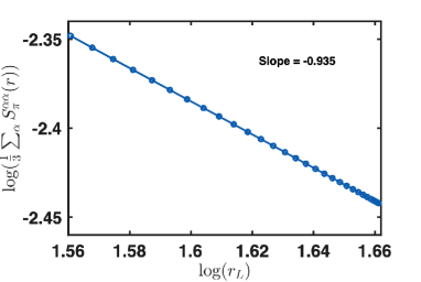
Figure 4: Averaged correlation function $\frac{1}{3}\sum_{\alpha=x,y,z}S^{\alpha\alpha}_{\pi}(r)$ as a function of $r_{L}=\frac{L}{\pi}\sin(\frac{\pi r}{L})$ on a log-log scale. DMRG numerics are performed on a system of $L=144$ sites with periodic boundary conditions where the bond dimension $m$ and truncation error $\epsilon$ are take as $m=1200$ and $\epsilon=10^{-9}$. The parameters in Eq. (42) are taken as $\theta=1.15\pi$, $D_{M}=0.3$.

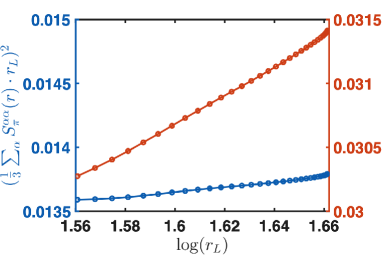
Figure 5: $[\frac{1}{3}\sum_{\alpha}S^{\alpha\alpha}_{\pi}(r)\cdot r_{L}]^{2}$ as a function of $\log r_{L}$ for $J_{2}=0$ (orange line) and $J_{2}=0.135$ (blue line). DMRG numerics are performed on a system of $L=144$ sites with a periodic boundary condition where the bond dimension $m$ and truncation error $\epsilon$ are take as $m=1200$ and $\epsilon=10^{-9}$. The parameters in Eq. (42) are taken as $\theta=1.15\pi$, $D_{M}=0.3$.

First, we study the spin correlation functions. By properly normalizing the WZW current operators and the primary field, the SU(2)₁ WZW model predicts the following static correlation functions,

$$\langle J^{\alpha}(0)J^{\beta}(r)\rangle = \delta_{\alpha\beta}\frac{1}{r^{2}},$$

$$\langle N^{\alpha}(0)N^{\beta}(r)\rangle = \delta_{\alpha\beta}\frac{(\ln(r/r_{0}))^{1/2}}{r},$$ (43)

in which $J^{\alpha}=J^{\alpha}_{L}+J^{\alpha}_{R}$; $\langle...\rangle$ represent the expectation value over the ground state; the time variable is taken as zero; the arguments in $J^{\alpha}$ and $N^{\alpha}$ are spatial coordinates; the logarithmic correction in $\langle N^{\alpha}(0)N^{\beta}(r)\rangle$ comes from the marginally irrelevant operator $-u\int\vec{J}_{L}\cdot\vec{J}_{R}$ in the low energy theory; and $r_{0}$ is an ultraviolet cutoff, which is of the same order as the lattice constant. Using Eq. (43) and the nonsymmorphic nonabelian bosonization formulas in Eqs. (32), we obtain

$$\langle S^{\alpha}_{i}S^{\beta}_{j+6n}\rangle=$$

$$\delta_{\alpha\beta}\big{[}-D_{i}^{\alpha\alpha}D_{j}^{\alpha\alpha}\frac{1}{r^{2}}+(-)^{r}C_{i}^{\alpha\alpha}C_{j}^{\alpha\alpha}\frac{\ln^{1/2}(r/r_{0})}{r}\big{]},$$ (44)

in which $1\leq i,j\leq 6$. As can be easily seen from Eq. (44), in the long distance limit $r\gg 1$, the staggered component of the correlation function with the $(-)^{r}$ oscillating factor dominates over the uniform component.

Fig. 4 shows $\frac{1}{3}\sum_{\alpha=x,y,z}S^{\alpha\alpha}_{\pi}(r)$ as a function of $r_{L}$ on a log-log scale, in which $\theta=1.15\pi$, $D_{M}=0.3$ defined in Eq. (42); $S^{\alpha\alpha}_{\pi}(r)$ is the $\pi$-wavevector oscillating component of the correlation function $\langle S^{\alpha}_{1}S^{\alpha}_{r}\rangle$ as a function of $r$; $r_{L}=\frac{L}{\pi}\sin(\frac{\pi r}{L})$ in accordance of CFT in finite size systems DiFrancesco1997 ; and DMRG numerics are performed on a system of $L=144$ sites with periodic boundary conditions where the bond dimension $m$ and truncation error $\epsilon$ are taken as $m=1200$ and $\epsilon=10^{-9}$. The slope of the line in Fig. 4 is extracted to be $-0.935$ by assuming a linear relation, which is pretty close to $-1$ as predicted by the SU(2)₁ CFT. In fact, the deviation from $-1$ originates from the logarithmic correction in Eq. (44).

To further study the logarithmic correction, we plot $[\frac{1}{3}\sum_{\alpha}S^{\alpha\alpha}_{\pi}(r)\cdot r_{L}]^{2}$ as a function of $\log r_{L}$ as shown by the orange line in Fig. 5. It can be observed that the line is linear with a non-vanishing slope, indicating a logarithmic correcting factor with a $1/2$ power in $S^{\alpha\alpha}_{\pi}(r)$.

In fact, the logarithmic correction can be killed by introducing a second nearest neighbor Heisenberg term Affleck1988 in the six-sublattice rotated frame. By introducing a $J_{2}$ term into Eq. (8), we consider the following Hamiltonian,

$$H^{\prime}_{2} = \sum_{\langle ij\rangle\in\gamma\,\text{bond}}\big{(}-KS_{i}^{\gamma}S_{j}^{\gamma}-\Gamma_{1}S_{i}^{\alpha}S_{j}^{\alpha}-\Gamma_{2}S_{i}^{\beta}S_{j}^{\beta}\big{)},$$ (45)

$$+J_{2}\sum_{i}\vec{S}_{i}\cdot\vec{S}_{i+2}.$$

The $J_{2}$ term renormalizes the coupling constant $u$ in the $\vec{J}_{L}\cdot\vec{J}_{R}$ term in Eq. (28). When $J_{2}$ is at a critical value $J_{c2}$, the coupling $u$ vanishes and the logarithmic correction is killed.

The blue line in Fig. 5 shows $[\frac{1}{3}\sum_{\alpha}S^{\alpha\alpha}_{\pi}(r)\cdot r_{L}]^{2}$ as a function of $\log r_{L}$ when $J_{2}$ is chosen as $J_{2}=0.135$. Clearly, the blue line has a significantly reduced slope compared with the orange line in the same figure, hinting a critical value $J_{c2}$ very close to $0.135$.

V.2 Central charge

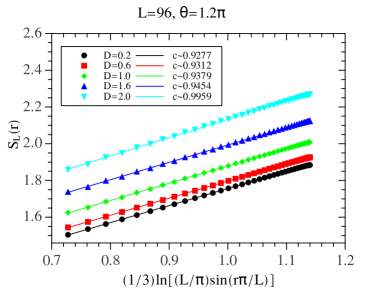
Figure 6: $S_{L}(r)$ as a function of $\frac{1}{3}\ln\left[\frac{L}{\pi}\sin\left(\frac{\pi r}{L}\right)\right]$ for a variety of $D_{M}$ at $\theta=1.2\pi$, where the parametrization is defined in Eq. (42). DMRG numerics are performed on a system of $L=96$ sites with a periodic boundary condition where the bond dimension $m$ and truncation error $\epsilon$ are taken as $m=1200$ and $\epsilon=10^{-8}$.

In this subsection, we study the central charge of the system. SU(2)₁ CFT predicts a central charge $c=1$. We will show the numerical evidence supporting this prediction in the emergent SU(2)₁ phase in Fig. 3. DMRG numerics are performed on a system of $L=96$ sites with periodic boundary conditions where the bond dimension $m$ and truncation error $\epsilon$ are taken as $m=1200$ and $\epsilon=10^{-8}$. The parameter $\theta$ in Eq. (42) is fixed to be $\theta=1.2\pi$, and $D_{M}$ is tuned.

We compute the entanglement entropy $S_{L}(x)$ of a subregion $x$ to extract the value of the central charge. Conformal field theory predicts the following scaling of the entanglement entropy Calabrese2009

$$S_{L}(r)=\frac{c}{3}\ln\left[\frac{L}{\pi}\sin\left(\frac{\pi r}{L}\right)\right]+\cdots.$$ (46)

Fig. 6 shows $S_{L}(r)$ vs. $\frac{1}{3}\ln\left[\frac{L}{\pi}\sin\left(\frac{\pi r}{L}\right)\right]$ for a variety of $D_{M}$ at $\theta=1.2\pi$. It is clear from Fig. 6 that the slopes are all very close to $1$, indicating $c=1$ in accordance with Eq. (46).

V.3 Scaling of the finite size gap

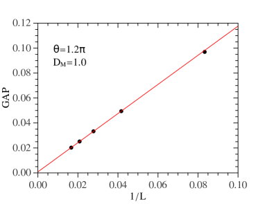
Figure 7: Excitation gap as a function of $1/L$ at $\theta=1.2\pi$, $D_{M}=1.0$.

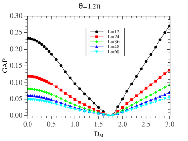
Figure 8: Excitation gap as a function of $D_{M}$ with fixed $\theta=1.2\pi$ for several system sizes marked with different colored lines.

In this section, we discuss the scaling of the finite size gap, which is predicted to be $\sim 1/L$ according to CFT.

Fig. 7 shows the excitation gap as a function of $1/L$ at $\theta=1.2\pi$, $D_{M}=1.0$, which is clearly very linear, consistent with the CFT prediction.

Fig. 8 shows the scaling of the gap by tuning $D_{M}$ where $\theta$ is fixed as $\theta=1.2\pi$. As can be seen from Fig. 8, the range of the emergent SU(2)₁ phase is rather large, except the narrow region for $D_{M}\in[1.68,1.80]$ where the $1/L$ scaling fails. We expect the regions for $D_{M}\leq 1.68$ and $D_{M}\geq 1.80$ in Fig. 8 to lie in the unitarily equivalent (under $R(\hat{z},\pi)$ in the original frame) counterparts of the “Emergent SU(2)₁ I” and “Emergent SU(2)₁ II” phases in Fig. 3, respectively, in the back half of the unit sphere.

V.4 Phase transitions

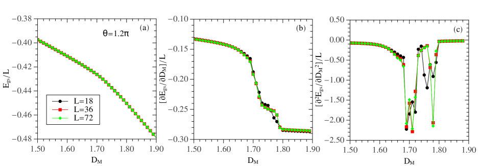
Figure 9: (a) Ground state energy per site $E_{gs}/L$, (b) first order derivative $\frac{1}{L}\frac{\partial E_{gs}}{\partial D_{M}}$, (c) second order derivative $\frac{1}{L}\frac{\partial^{2}E_{gs}}{\partial D_{M}^{2}}$ as functions of $D_{M}$ for $L=18$ (black), $L=36$ (red) and $L=72$ (green) at $\theta=1.2\pi$.

In this subsection, we take a closer look at the region $D_{M}\in[1.68,1.80]$ in Fig. 8, where the system does not show a Luttinger liquid behavior.

Fig. 9 (a), (b), (c) show the ground state energy per site $E_{gs}/L$, the first order derivative $\frac{1}{L}\frac{\partial E_{gs}}{\partial D_{M}}$, and the second order derivative $\frac{1}{L}\frac{\partial^{2}E_{gs}}{\partial D_{M}^{2}}$, respectively, as functions of $D_{M}$, at $\theta=1.2\pi$. Interestingly, there seems to be several different phases in the narrow region $D_{M}\in[1.68,1.80]$, which separates the two emergent SU(2)₁ phases. More investigations on the physics in this narrow region will be left for future studies.

VI Summary

In summary, we have studied the spin-1/2 Kitaev-Gamma chain with a bond-dependent Dzyaloshinskii-Moriya interaction. Using a two-site periodic unitary transformation which maps the Gamma and Dzyaloshinskii-Moriya terms into one another, the phase diagram of a pure Kitaev chain with a Dzyaloshinskii-Moriya term is obtained from the known results of the Kitaev-Gamma model. More importantly, we are able to analytically demonstrate that there is an extended gapless phase in the phase diagram of the spin-1/2 Kitaev-Gamma chain with a nonzero Dzyaloshinskii-Moriya interaction, and such gapless phase has an emergent SU(2)₁ conformal symmetry at low energies. The analytical predictions are supported by density matrix renormalization group simulations. Our work is useful to understand the effects of the Dzyaloshinskii-Moriya interactions and the electric fields in one-dimensional and quasi-one-dimensional generalized Kitaev spin models.

Appendix A Staggered second nearest neighbor coupling

We make some further comments about the $(\vec{J}_{L}+\vec{J}_{R})\cdot\vec{N}$ term. As can be seen from Eq. (23), the $(\vec{J}_{L}+\vec{J}_{R})\cdot\vec{N}$ term vanishes at the hidden SU(2)₁ symmetric point where $D_{1}=D_{2}$, $C_{1}=C_{2}$. In fact, the appearance of $(\vec{J}_{L}+\vec{J}_{R})\cdot\vec{N}$ is an unusual feature of the Kitaev-Gamma model arising from the nonsymmorphic symmetries. It can appear in the SU(2) symmetric AFM Heisenberg model only at second nearest neighbor level. The nonabelian bosonization formulas of the spin operators for the SU(2) symmetric case (i.e., $D_{1}=D_{2}$, $C_{1}=C_{2}$) are

$$\frac{1}{a}S_{i}^{\alpha}=J_{L}^{\alpha}+J_{R}^{\alpha}+(-)^{i+1}\frac{c}{2\pi a}N^{\alpha},$$ (47)

where $c$ is a constant. Plugging Eq. (47) and Eq. (20) into $S_{i}^{\alpha}S_{i+2}^{\alpha}$, we obtain

$$S_{i}^{\alpha}S_{i+2}^{\alpha} = a^{2}[J_{L}^{\alpha}(x)J_{L}^{\alpha}(x+2a)+J_{R}^{\alpha}(x)J_{R}^{\alpha}(x+2a)$$ (48)

$$+2J_{L}^{\alpha}(x)J_{R}^{\alpha}(x+2a)]$$

$$+(-)^{i+1}\frac{ca}{\pi}(:J_{L}^{\alpha}N^{\alpha}:+:J_{R}^{\alpha}N^{\alpha}:)$$

$$+\frac{c^{2}}{4\pi^{2}}N^{\alpha}(x)N^{\alpha}(x+2a).$$

Using Eq. (48), it is clear that

$$(-)^{i+1}S^{\alpha}_{i}S^{\alpha}_{i+2}+(-)^{i+2}S^{\alpha}_{i+1}S^{\alpha}_{i+3}=\frac{2ca}{\pi}:(J^{\alpha}_{L}+J^{\alpha}_{R})N^{\alpha}:,$$ (49)

which shows that $:(J^{\alpha}_{L}+J^{\alpha}_{R})N^{\alpha}:$ corresponds to a staggered second nearest neighbor coupling in the AFM Heisenberg model.

Appendix B $(\vec{J}_{L}+\vec{J}_{R})\cdot\vec{N}$ as a total derivative

In this appendix, we give a formal proof that $:(J^{\alpha}_{L}+J^{\alpha}_{R})N^{\alpha}:$ is a total derivative within the SU(2)₁ low energy theory Since the Hamiltonian in the holomorphic and anti-holomorphic sectors are of the Sugawara form which generates the translations, we have

$$[\frac{1}{3}\int dx:\vec{J}_{L}\cdot\vec{J}_{L}:,g(w,\bar{w})] = \partial_{w}g(w,\bar{w}),$$ (50)

and

$$[\frac{1}{3}\int dx:\vec{J}_{R}\cdot\vec{J}_{R}:,g(w,\bar{w})] = \partial_{\bar{w}}g(z,\bar{w}).$$ (51)

In what follows, we focus on the holomorphic sector, as the treatment for the anti-holomorphic sector is similar. For simplification of notation, we write the normal order product $:AB:$ as $(AB)$ in accordance with the notation in Ref. DiFrancesco1997, .

The commutator in Eq. (50) can be deformed to a small loop centering around the point $w$ as

$$\partial_{w}g(w,\bar{w}) = \frac{1}{3}\sum_{\alpha}\oint_{w}dy(J_{L}^{\alpha}J_{L}^{\alpha})(y)g(w,\bar{w}).$$ (52)

To evaluate Eq. (52), we need the $\frac{1}{y-w}$ term in the OPE $(J_{L}^{\alpha}J_{L}^{\alpha})(y)g(w,\bar{w})$. Define $\contraction{}{A}{(z)}{B}A(z)B(w)$ to be the singular parts of the OPE $A(z)B(w)$, i.e., the terms with coefficients $(y-w)^{-n}$ where $n\geq 1$. According to the generalized Wick’s theorem in Ref. DiFrancesco1997, , the singular terms in the OPE $(J_{L}^{\alpha}J_{L}^{\alpha})(y)g(w,\bar{w})$ can be evaluated as

$$\contraction{(J_{L}^{\alpha}}{J}{{}_{L}^{\alpha})(y)}{g}\contraction{(J_{L}^{\alpha}J_{L}^{\alpha})(y)g(w,\bar{w})=\frac{1}{2\pi i}\oint_{y}\frac{dz}{z-y}\big{[}J_{L}^{\alpha}(z)}{J}{{}_{L}^{\alpha}(y)}{g}\contraction{(J_{L}^{\alpha}J_{L}^{\alpha})(y)g(w,\bar{w})=\frac{1}{2\pi i}\oint_{y}\frac{dz}{z-y}\big{[}J_{L}^{\alpha}(z)J_{L}^{\alpha}(y)g(w,\bar{w})+}{J}{{}_{L}^{\alpha}(z)}{g}(J_{L}^{\alpha}J_{L}^{\alpha})(y)g(w,\bar{w})=\frac{1}{2\pi i}\oint_{y}\frac{dz}{z-y}\big{[}J_{L}^{\alpha}(z)J_{L}^{\alpha}(y)g(w,\bar{w})+J_{L}^{\alpha}(z)g(w,\bar{w})J_{L}^{\alpha}(y)\big{]}.$$ (53)

Using Eq. (19), Eq. (53) becomes

$$\frac{1}{2\pi i}\oint_{y}\frac{dz}{z-y}(-\frac{1}{2})\big{[}\frac{\sigma^{\alpha}J_{L}^{\alpha}(z)g(w,\bar{w})}{y-w}+\frac{\sigma^{\alpha}g(w,\bar{w})J_{L}^{\alpha}(y)}{z-w}\big{]}.$$ (54)

Further using Eq. (19), we obtain

$$\frac{g(w,\bar{w})}{2(y-w)^{2}}-\frac{\sigma^{\alpha}(J^{\alpha}_{L}g)(w,\bar{w})}{y-w}.$$ (55)

Notice that only the $1/(y-w)$ term in Eq. (55) contributes to Eq. (52), leading to

$$\partial_{w}g(w,\bar{w})=-\frac{1}{3}\sum_{\alpha}\sigma^{\alpha}(J^{\alpha}_{L}g)(w,\bar{w}).$$ (56)

Taking the trace of Eq. (56), we arrive at

$$i\partial_{w}\epsilon(w,\bar{w})=-\frac{1}{3}(\vec{J}_{L}\cdot\vec{N})(w,\bar{w}).$$ (57)

Similar calculations in the anti-holomorphic sector gives

$$i\partial_{\bar{w}}\epsilon(w,\bar{w})=\frac{1}{3}(\vec{J}_{R}\cdot\vec{N})(w,\bar{w}).$$ (58)

Hence

$$((\vec{J}_{L}+\vec{J}_{R})\cdot\vec{N})(w,\bar{w})=-3i(\partial_{w}-\partial_{\bar{w}})\epsilon(w,\bar{w}).$$ (59)

Notice that $\partial_{z}-\partial_{\bar{z}}=-i\partial_{x}$, therefore

$$\int dx((\vec{J}_{L}+\vec{J}_{R})\cdot\vec{N})=-3\int dx\partial_{x}\epsilon,$$ (60)

which clearly vanishes.

Appendix C Symmetry transformations of the WZW fields

As discussed in Ref. Yang2020, , the symmetry transformation properties of the WZW fields $g$ and $\vec{J_{L}},\vec{J}_{R}$ under time reversal $T$, spatial translation $T_{a}$, inversion $I$ and global spin rotation $R$ ($\in SO(3)$) are given by

$$T: \epsilon(x)\rightarrow\epsilon(x), \vec{N}(x)\rightarrow-\vec{N}(x),$$ (61)

$$\vec{J}_{L}(x)\rightarrow-\vec{J}_{R}(x), \vec{J}_{R}(x)\rightarrow-\vec{J}_{L}(x),$$

$$T_{a}: \epsilon(x)\rightarrow-\epsilon(x), \vec{N}(x)\rightarrow-\vec{N}(x),$$ (62)

$$\vec{J}_{L}(x)\rightarrow\vec{J}_{L}(x), \vec{J}_{R}(x)\rightarrow\vec{J}_{R}(x),$$

$$I: \epsilon(x)\rightarrow-\epsilon(-x), \vec{N}(x)\rightarrow\vec{N}(-x),$$ (63)

$$\vec{J}_{L}(x)\rightarrow\vec{J}_{R}(-x), \vec{J}_{R}(x)\rightarrow\vec{J}_{L}(-x),$$

$$R: \epsilon(x)\rightarrow\epsilon(x), N^{\alpha}(x)\rightarrow R^{\alpha}_{\,\,\beta}N^{\beta}(x),$$ (64)

$$J^{\alpha}_{L}(x)\rightarrow R^{\alpha}_{\,\,\beta}J^{\beta}_{L}(x), J^{\alpha}_{R}(x)\rightarrow R^{\alpha}_{\,\,\beta}J^{\beta}_{R}(x).$$

in which $x$ is the spatial coordinate, and $R^{\alpha}_{\,\,\beta}$ ($\alpha,\beta=x,y,z$) is the matrix element of the $3\times 3$ rotation matrix $R$ at position $(\alpha,\beta)$.

References

- (1) A. Kitaev, Ann. Phys. (N. Y). 321, 2 (2006).
- (2) C. Nayak, S. H. Simon, A. Stern, M. Freedman, and S. Das Sarma, Rev. Mod. Phys. 80, 1083 (2008).
- (3) G. Jackeli and G. Khaliullin, Phys. Rev. Lett. 102, 017205 (2009).
- (4) J. Chaloupka, G. Jackeli, and G. Khaliullin, Phys. Rev. Lett. 105, 027204 (2010).
- (5) Y. Singh and P. Gegenwart, Phys. Rev. B 82, 064412 (2010).
- (6) C. C. Price and N. B. Perkins, Phys. Rev. Lett. 109, 187201 (2012).
- (7) Y. Singh, S. Manni, J. Reuther, T. Berlijn, R. Thomale, W. Ku, S. Trebst, and P. Gegenwart, Phys. Rev. Lett. 108, 127203 (2012).
- (8) K. W. Plumb, J. P. Clancy, L. J. Sandilands, V. V. Shankar, Y. F. Hu, K. S. Burch, H. Y. Kee, and Y. J. Kim, Phys. Rev. B 90, 041112 (2014).
- (9) H.-S. Kim, V. S. V., A. Catuneanu, and H.-Y. Kee, Phys. Rev. B 91, 241110 (2015).
- (10) S. M. Winter, Y. Li, H. O. Jeschke, and R. Valenti, Phys. Rev. B 93, 214431 (2016).
- (11) S. H. Baek, S. H. Do, K. Y. Choi, Y. Kwon, A. Wolter, S. Nishimoto, J. van den Brink, and B. Buchner, Phys. Rev. Lett. 119, 037201 (2017).
- (12) I. A. Leahy, C. A. Pocs, P. E. Siegfried, D. Graf, S. H. Do, K. Y. Choi, B. Normand, and M. Lee, Phys. Rev. Lett. 118, 187203 (2017).
- (13) J. A. Sears, Y. Zhao, Z. Xu, J. W. Lynn, and Y. J. Kim, Phys. Rev. B 95, 180411 (2017).
- (14) A. U. B. Wolter, L. T. Corredor, L. Janssen, K. Nenkov, S. Schonecker, S. H. Do, K. Y. Choi, R. Albrecht, J. Hunger, T. Doert, M. Vojta, and B. Buchner, Phys. Rev. B 96, 041405(R) (2017).
- (15) J. Zheng, K. Ran, T. Li, J. Wang, P. Wang, B. Liu, Z.-X. Liu, B. Normand, J. Wen, and W. Yu, Phys. Rev. Lett. 119, 227208 (2017).
- (16) I. Rousochatzakis and N. B. Perkins, Phys. Rev. Lett. 118, 147204 (2017).
- (17) Y. Kasahara, T. Ohnishi, N. Kurita, H. Tanaka, J. Nasu, Y. Motome, T. Shibauchi, and Y. Matsuda, Nature (London) 559, 227 (2018).
- (18) J. G. Rau, E. K. H. Lee, and H. Y. Kee, Phys. Rev. Lett. 112, 077204 (2014).
- (19) K. Ran, J. Wang, W. Wang, Z.-Y. Dong, X. Ren, S. Bao, S. Li, Z. Ma, Y. Gan, Y. Zhang, J. T. Park, G. Deng, S. Danilkin, S.-L. Yu, J.-X. Li, and J. Wen, Phys. Rev. Lett. 118, 107203 (2017).
- (20) W. Wang, Z.-Y. Dong, S.-L. Yu, and J.-X. Li, Phys. Rev. B 96, 115103 (2017).
- (21) A. Catuneanu, Y. Yamaji, G. Wachtel, Y. B. Kim, and H.-Y. Kee, npj Quantum Mater. 3, 23 (2018).
- (22) M. Gohlke, G. Wachtel, Y. Yamaji, F. Pollmann, and Y. B. Kim, Phys. Rev. B 97, 075126 (2018).
- (23) X. Liu, T. Berlijn, W.-G. Yin, W. Ku, A. Tsvelik, Young-June Kim, H. Gretarsson, Yogesh Singh, P. Gegenwart, and J. P. Hill, Phys. Rev. B 83, 220403(R) (2011).
- (24) J. Chaloupka, G. Jackeli, and G. Khaliullin, Phys. Rev. Lett. 110, 097204 (2013).
- (25) R. D. Johnson, S. C. Williams, A. A. Haghighirad, J. Singleton, V. Zapf, P. Manuel, I. I. Mazin, Y. Li, H. O. Jeschke, R. Valentí, and R. Coldea, Phys. Rev. B 92, 235119 (2015).
- (26) Motome, R. Sano, S. H. Jang, Y. Sugita, and Y. Kato, J. Phys.: Condens. Matter 32, 404001 (2020).
- (27) E. Sela, H.-C. Jiang, M. H. Gerlach, and S. Trebst, Phys. Rev. B 90, 035113 (2014).
- (28) C. E. Agrapidis, J. van den Brink, and S. Nishimoto, Sci. Rep. 8, 1815 (2018).
- (29) C. E. Agrapidis, J. van den Brink, and S. Nishimoto, Phys. Rev. B 99, 224418 (2019).
- (30) A. Catuneanu, E. S. Sørensen, and H.-Y. Kee, Phys. Rev. B 99, 195112 (2019).
- (31) W. Yang, A. Nocera, T. Tummuru, H.-Y. Kee, and I. Affleck, Phys. Rev. Lett. 124, 147205 (2020).
- (32) W. Yang, A. Nocera, and I. Affleck, Phys. Rev. Research 2, 033268 (2020).
- (33) W. Yang, A. Nocera, and I. Affleck, Phys. Rev. B 102, 134419 (2020).
- (34) W. Yang, A. Nocera, E. S. Sørensen, H.-Y. Kee, and I. Affleck, Phys. Rev. B 103, 054437 (2021).
- (35) W. Yang, A. Nocera, P. Herringer, R. Raussendorf, I. Affleck, Phys. Rev. B 105, 094432 (2022).
- (36) W. Yang, C. Xu, S. Xu, A. Nocera, I. Affleck, arXiv:2202.11686 (2022).
- (37) W. Yang, C. Xu, A. Nocera, I. Affleck, arXiv:2204.05441 (2022).
- (38) Q. Luo, J. Zhao, X. Wang, and H.-Y. Kee, Phys. Rev. B 103, 144423(2021).
- (39) Q. Luo, S. Hu, and H.-Y. Kee, Phys. Rev. Research 3, 033048 (2021).
- (40) Z.-A. Liu, T.-C. Yi, J.-H. Sun, Y.-L. Dong, and W.-L. You, Phys. Rev. E 102, 032127 (2020).
- (41) E. S. Sørensen, A. Catuneanu, J. Gordon, H.-Y. Kee, Phys. Rev. X 11, 011013 (2021).
- (42) I. E. Dzyaloshinskii, Zh. Eksp. Teor. Fiz. 32, 1547 (1957) [Sov. Phys. JETP 5, 1259 (1957)].
- (43) I. E. Dzyaloshinskii, Zh. Eksp. Teor. Fiz. 46, 1420 (1964) [Sov. Phys. JETP 19, 960 (1964)].
- (44) T. Moriya, Phys. Rev. 120, 91 (1960).
- (45) A. Fert and P. M. Levy, Phys. Rev. Lett. 44, 1538 (1980).
- (46) A. Fert, Mater. Sci. Forum 59-60, 439 (1990).
- (47) S. Heinze, K. von Bergmann, M. Menzel, J. Brede, A. Kubetzka, R. Wiesendanger, G. Bihlmayer, and S. Blügel, Nat. Phys. 7, 713 (2011).
- (48) X. Z. Yu, Y. Onose, N. Kanazawa, J. H. Park, J. H. Han, Y. Matsui, N. Nagaosa, and Y. Tokura, Nature (London) 465, 901 (2010).
- (49) A. Bogdanov and A. Hubert, J. Magn. Magn. Mater. 138, 255 (1994).
- (50) U. K. Rößler, A. N. Bogdanov, and C. Pfleiderer, Nature (London) 442, 797 (2006).
- (51) I. E. Dzyaloshinskii, Zh. Eksp. Teor. Fiz. 47, 992 (1964) [Sov. Phys. JETP 20, 665 (1965).
- (52) A. N. Bogdanov and D. A. Yablonskii, Zh. Eksp. Teor. Fiz. 95, 178 (1989) [Sov. Phys. JETP 68, 101 (1989)].
- (53) S. C. Furuya, M. Sato, arXiv:2110.06503 (2021).
- (54) R. Chari, R. Moessner, and J. G. Rau, Phys. Rev. B 103, 134444 (2021).
- (55) P. Francesco, P. Mathieu, and D. Sénéchal, Conformal Field Theory (Springer-Verlag, Berlin, 1997).
- (56) T. Giamarchi, Quantum Physics in One Dimension (Clarendon, Oxford, 2004).
- (57) I. Affleck, in Fields, Strings and Critical Phenomena, Proceedings of Les Houches Summer School, 1988, edited by E. Brezin and J. Zinn-Justin (North-Holland, Amsterdam, 1990), pp. 563-640.
- (58) P. Calabrese and J. Cardy, J. Phys. A 42, 504005 (2009).