Practical Considerations in Direct Detection Under Tukey Signalling

Abstract

The deliberate introduction of controlled intersymbol interference (ISI) in Tukey signalling enables the recovery of signal amplitude and (in part) signal phase under direct detection, giving rise to significant data rate improvements compared to intensity modulation with direct detection (IMDD). The use of an integrate-and-dump detector makes precise waveform shaping unnecessary, thereby equipping the scheme with a high degree of robustness to nonlinear signal distortions introduced by practical modulators. Signal sequences drawn from star quadrature amplitude modulation (SQAM) formats admit an efficient trellis description that facilitates codebook design and low-complexity near maximum-likelihood sequence detection in the presence of both shot noise and thermal noise. Under the practical (though suboptimal) allocation of a $50$% duty cycle between ISI-free and ISI-present signalling segments, at a symbol rate of $50~{}$Gbaud and a launch power of $-10~{}$dBm the Tukey scheme has a maximum theoretically achievable throughput of $200~{}$Gb/s with an $(8,4)$-SQAM constellation, while an IMDD scheme achieves about $145~{}$Gb/s using PAM-$8$. Note that the two mentioned constellations have the same number of magnitude levels and the difference in throughput is resulting from exploiting phase information under using a complex-valued signal constellation.

I Introduction

Tukey waveforms are time-limited signals that allow amplitude and (to some extent) phase recovery of complex-valued symbols under direction detection by the deliberate introduction of inter-symbol interference (ISI) [1], in a manner that is reminiscent of partial-response signalling schemes dating back to the early 1960s [2, 3]. Under Tukey signalling, ISI is controlled so that only adjacent symbols interfere, resulting in an alternation between ISI-free and ISI-present signalling segments at the receiver, where detection is accomplished by a low-complexity integrate-and-dump architecture.

Tukey signalling with direct detection is an alternative to intensity-modulation with direct detection (IMDD), which encodes only the intensity, i.e., squared magnitude, of the transmitted waveform by transmitting only positive real symbols. In contrast to IMDD, Tukey signalling with direct detection allows information to be encoded in the phase, not only the intensity, of the transmitted symbols; however, this increased capability necessitates implementation of an in-phase/quadrature (IQ) modulator at the transmitter and the use of two (rather than one) analog-to-digital (A/D) converters (each operating at the symbol rate) at the receiver. The requirement of having at least two real-valued samples per complex-valued symbol is inevitable in all schemes that extract phase (in addition to magnitude).

Another class of communication schemes that can exploit phase under direct detection is based on the so-called Kramers-Kronig (KK) (or Hilbert transform) relationship between the phase and the logarithm of the magnitude of a minimum-phase complex-valued signal [4, 5, 6]. The use of this relationship in communication systems dates back to the early 1960s [7, 8, 9, 10, 11, 12], where it was used to extract phase information from an envelope detector. To satisfy the minimum-phase constraint, KK-based schemes must add a non-information-bearing tone to the complex-valued waveform (either at the transmitter or at the receiver), resulting in a substantial inefficiency in overall transceiver power consumption. Furthermore, because they must perform bandwidth-broadening nonlinear operations, KK receivers often demand an over-sampling of about three times the minimum required sampling rate, i.e., six times the symbol rate. Although there are KK schemes that enable phase recovery without such oversampling, these require a very high carrier-to-signal power ratio [6].

In this paper, we address a number of practical concerns that arise with Tukey signalling under direct detection. In particular,

• we consider the influence of the nonlinearity of the IQ modulator (which was idealized in [1]) and show that the scheme is quite robust to modulator imperfections;

• we fix the duty-cycle between ISI-free and ISI-present signalling segments to $50\%$ (unlike in [1], where it was allowed to range to values as low as $10\%$, which leads to unrealistically short integration intervals in high baud-rate systems);

• we introduce a low-complexity near maximum-likelihood (ML) trellis-based decoding algorithm in the presence of both shot noise and thermal noise encountered at the output of a p-i-n photodiode under practical parameter settings (replacing the brute-force search decoding and avalanche photodiode analysis of [1]);

• we consider a wider range of constellation sizes compared with [1].

The rest of the paper is organized as follows. Sec. II describes the system model for use in the C band where chromatic dispersion is significant; in particular, Sec. II-B addresses the nonlinearity of the IQ modulator. Sec. III shows how trellis diagrams can be used for codebook design and decoding. While typically trellises are associated with a given codebook, in Sec. III-D trellises are used to find codebooks composed of symbols drawn from the class of signal constellations described in Sec. III-B. Sec. III-E provides a branch-metric function that enables near-ML trellis-based decoding using the Viterbi algorithm. Sec. IV provides extensive numerical simulation results, while Sec. V compares Tukey signalling under direct detection with IMDD. The system model of Sec. II requires link-distance knowledge to precompensate for chromatic dispersion. In Sec. VI, we remove this requirement by operating in the O band, instead of the C band, leaving residual chromatic dispersion uncompensated and making the transmitter agnostic to the transmission-link length. Finally, Sec. VII provides various concluding remarks.

Throughout this paper, the integers, real numbers, and complex numbers are denoted, respectively, by $\mathbb{Z}$, $\mathbb{R}$, and $\mathbb{C}$. The set of real-valued and complex-valued functions over $\mathbb{R}$ are denoted as $\mathbb{R}^{\mathbb{R}}$ and $\mathbb{C}^{\mathbb{R}}$, respectively. For any $x\in\mathbb{R}$, $\mathbb{R}^{>x}$ denotes the set of real numbers strictly greater than $x$. The sets $\mathbb{R}^{\geq x}$, $\mathbb{Z}^{>x}$, and $\mathbb{Z}^{\geq x}$ are defined similarly. For any $a,b\in\mathbb{Z}$ with $a\leq b$, let $\llbracket{a},{b}\rrbracket=\{a,a+1,\ldots,b\}$. The cardinality of a set $\mathcal{S}$ is denoted by $|\mathcal{S}|$; thus, e.g., $|\llbracket{0},{m-1}\rrbracket|=m$. For any $r\in\mathbb{R}$, $\lceil r\rceil$ and $\lfloor r\rfloor$ denote, respectively, the smallest integer greater than or equal to $r$ and the largest integer less than or equal to $r$. For a complex number $w\in\mathbb{C}$, $|w|$, $\arg(w)$, and $w^{\ast}$ denote the magnitude, phase, and complex conjugate of $w$, respectively; furthermore, we assume that $\arg(w)\in[0,2\pi)$ and $i=\sqrt{-1}$. The Fourier transform of a complex-valued function $x(t)$ is denoted as $\mathcal{F}[x(t)]$; the inverse Fourier transform of $X(f)$ is denoted as $\mathcal{F}^{-1}[X(f)]$. For a random variable $X$, $X\sim\mathcal{N}(\mu,\sigma^{2})$ denotes that $X$ has a Gaussian distribution with mean $\mu$ and variance $\sigma^{2}$. Finally, for any $k\in\mathbb{Z}^{>0}$, $\bm{I}_{k}$ denotes the $k\times k$ identity matrix, while for any $k$ and $\ell\in\mathbb{Z}^{>0}$, $\mathds{1}_{k\times\ell}$ denotes the all-one matrix of size $k\times\ell$.

II System Model

In this section, we describe the system model, as shown in Fig. 1. For simplicity of computations and ease of reading, we assume transmission over a single polarization; however, with an obvious modification, the scheme can be adapted to work in a dual-polarized system.

Figure 1: The system model for operation in the C band. For the O band system model, see Fig. 13.

II-A The Transmission Medium

We assume data transmission over a standard single-mode fiber (SSMF) at a wavelength in the C band, i.e., close to $1550~{}$nm, where the fiber has the lowest loss, i.e., about $0.2~{}\text{dB}\cdot\text{km}^{-1}$. The lower loss comes at the expense of a higher chromatic dispersion compared to operating at the zero-dispersion wavelength of SSMF, i.e., about $1310~{}$nm in the O band.

A key application of direct detection is in short-haul data transmission, e.g., intra data-center communication. Therefore, power loss and chromatic dispersion are the only fiber imperfections that we take into account. Other defects of the channel, e.g., Kerr effect or polarization mode dispersion (for a dual-polarized transmission), are not considered. Accordingly, if the waveform $x(t)\in\mathbb{C}^{\mathbb{R}}$ is launched into the fiber, the waveform received at the fiber output is modelled as [13, Sec. 4.3.3]

$$r(t)=\mathcal{F}^{-1}\left[X(f)e^{-\varrho\frac{L}{2}}e^{-i\beta_{0}L}e^{-2\pi f\beta_{1}L}e^{-i2\beta_{2}L\pi^{2}f^{2}}\right],$$

where $X(f)=\mathcal{F}[x(t)]$, $L\in\mathbb{R}^{>0}$ is the fiber length, $\varrho\in\mathbb{R}^{>0}$ is the loss factor and $\beta_{2}\in\mathbb{R}$ is the group-velocity dispersion parameter. At the wavelength of $1550~{}$nm, $\varrho=0.046~{}\text{km}^{-1}$ (equivalent to a loss of $0.2~{}\text{dB}\cdot\text{km}^{-1}$) and $\beta_{2}=-2.167\times 10^{-23}~{}\text{s}^{2}\cdot\text{km}^{-1}$. At the operating wavelength $\lambda$, we have $\beta_{0}=2\pi/\lambda$. Furthermore, $\beta_{1}$ is the group delay per unit of length [13, Sec. 4.3].

II-B IQ Modulator

The IQ modulator comprises two Mach-Zehnder modulators (MZMs) operating in the push-pull regime. For a modulating waveform $v(t)\in\mathbb{R}^{\mathbb{R}}$, the output of an MZM in this regime is $E_{\text{out}}(t)=E_{\text{in}}\sin\left(\kappa v(t)\right)$, where $E_{\text{in}}$ is an unmodulated continuous-wave narrow-band optical input and $\kappa\in\mathbb{R}$ is a constant depending on the operating wavelength and physical properties of the MZM [13, Sec. 7.5.3]. In this paper, we consider a baseband model; thus, we assume that $E_{\text{in}}\in\mathbb{R}^{>0}$. The IQ modulator uses separate MZMs for the in-phase and the quadrature components, producing the optical waveform [13, Sec. 7.5.3]

$$x(t)=E_{\text{in}}\Big{(}\sin\left(\kappa\operatorname{Re}\left(u(t)\right)\right)+i\sin\left(\kappa\operatorname{Im}\left(u(t)\right)\right)\Big{)}$$ (1)

in response to the complex-valued electrical waveform $u(t)\in\mathbb{C}^{\mathbb{R}}$.

II-C Signalling

For any $\beta\in[0,1]$ the Tukey (or time-domain raised cosine [14]) waveform $w_{\beta}(t)$ is defined as [1]

$$w_{\beta}(t)\triangleq\begin{cases}\alpha_{\beta},&\text{if }|t|\leq\frac{(1-\beta)}{2};\\ \frac{\alpha_{\beta}}{2}\left(1-\sin\left(\frac{\pi(2|t|-1)}{2\beta}\right)\right),&\text{if }\left||t|-\frac{1}{2}\right|\leq\frac{\beta}{2};\\ 0,&\text{otherwise},\end{cases}$$

where $\alpha_{\beta}\triangleq\frac{2}{\sqrt{4-\beta}}$. For a $T\in\mathbb{R}^{>0}$ and a block length $n\in\mathbb{Z}^{>1}$, the signalling block in Fig. 1 accepts $n$ complex numbers $x_{0},\ldots,x_{n-1}\in\mathbb{C}$ as its input and produces

$$g(t)=\sum_{k\in\llbracket{0},{n-1}\rrbracket}x_{k}w(t-kT),$$ (2)

where the signalling waveform $w(t)$ is a scaled, dilated Tukey waveform; in particular, $w(t)=\frac{1}{\sqrt{T}}w_{\beta}(\frac{t}{T})$ for some $\beta\in[0,1]$.

II-D Dispersion Precompensation

Chromatic dispersion is precompensated in the electrical domain by a filter with frequency response $H(f)=e^{i2\beta_{2}L\pi^{2}f^{2}}$. Note that this linear precompensation does not take into account the nonlinearity of the IQ modulator and therefore it does not perform ideal precompensation. Nevertheless, when the power of the modulating waveform, $u(t)$, is relatively small, the IQ modulator operates almost linearly; thus, the dispersion precompensating filter with frequency response $H(f)$ compensates the chromatic dispersion of the fiber to a large degree.

II-E Photodiode and Noise

The output $s(t)\in\mathbb{R}^{\mathbb{R}}$ of the photodiode, in response to the input waveform $r(t)\in\mathbb{C}^{\mathbb{R}}$, is given as

$$s(t)=\mathfrak{R}\,|r(t)|^{2}+|r(t)|n_{\text{sh}}(t)+n_{\text{th}}(t),$$

where $\mathfrak{R}$ is the photodiode responsivity, and where $n_{\text{sh}}(\cdot)$ and $n_{\text{th}}(\cdot)$ are zero-mean white Gaussian random processes with constant two-sided power spectral densities $\sigma_{\text{sh}}^{2}$ and $\sigma_{\text{th}}^{2}$, respectively. The two terms, $|r(t)|n_{\text{sh}}(t)$ and $n_{\text{th}}(t)$, are referred to as shot noise and thermal noise, respectively.

II-F Integrate & Dump

Note that $g(t)$ depends only on $x_{k}$, $k\in\llbracket{0},{n-1}\rrbracket$, whenever $\left|t-kT\right|\leq\frac{(1-\beta)T}{2}$ and depends only on $x_{\ell}$ and $x_{\ell+1}$, $\ell\in\llbracket{0},{n-2}\rrbracket$, whenever $\left|t-(\ell+\frac{1}{2})T\right|\leq\frac{1}{2}\beta T$. Thus, as in [1], we define the $k^{\text{th}}$ ISI-free interval as

$$\mathcal{Y}_{k}\triangleq\{t\in\mathbb{R}\colon|t-kT|\leq(1-\beta)T/2\}$$

and the $\ell^{\text{th}}$ ISI-present interval as

$$\mathcal{Z}_{\ell}\triangleq\{t\in\mathbb{R}\colon|t-\ell T-T/2|<\beta T/2\}.$$

The integrate-and-dump unit accepts $s(t)$ as its input and produces

$$y_{k}=\int_{\mathcal{Y}_{k}}s(t)~{}\text{d}t\quad\text{ and }\quad z_{\ell}=\int_{\mathcal{Z}_{\ell}}s(t)~{}\text{d}t$$ (3)

for $k\in\llbracket{0},{n-1}\rrbracket$ and $\ell\in\llbracket{0},{n-2}\rrbracket$.

As we do not compensate for the nonlinearity of the IQ modulator, determining the exact distribution of $y_{k}$ and $z_{\ell}$ given the transmitted symbols, $x_{0},\ldots,x_{n-1}$, is not straightforward. Thus, the implementation of a true ML receiver seems intractable. Instead, we use

$$x(t)\simeq E_{\text{in}}\kappa u(t),$$ (4)

as an approximation for (1) at the decoder, which becomes increasingly accurate for low-power modulating waveforms. Note that this approximation is applied at the receiver, and not at the transmitter, to simplify computations. In all simulation results reported in Sec. IV, the nonlinearity of the IQ modulator, as given in (1), has been properly taken into account when simulating the transmitter.

Using (4), one may approximate $y_{k}$ in (3) as

$$y_{k}\simeq\mathfrak{R}\,\overline{y_{k}}+\sqrt{\overline{y_{k}}}n_{k}+m_{k},$$ (5)

where

$$\overline{y_{k}}=\left(E_{\text{in}}\kappa\alpha_{\beta}e^{-\varrho\frac{L}{2}}|x_{k}|\right)^{2}(1-\beta)\in\mathbb{R}^{\geq 0},$$ (6)

and where $n_{k}\sim\mathcal{N}(0,\sigma_{\text{sh}}^{2})$, $m_{k}\sim\mathcal{N}(0,(1-\beta)T\sigma_{\text{th}}^{2})$, and $k\in\llbracket{0},{n-1}\rrbracket$.

Define $\psi:\mathbb{C}^{2}\rightarrow\mathbb{R}^{\geq 0}$ such that, for all $(a,b)\in\mathbb{C}^{2}$,

$$\psi(a,b)=\frac{1}{4}|a+b|^{2}+\frac{1}{8}|a-b|^{2}.$$ (7)

Note that $\psi(a,b)$ is a function of the magnitudes of $a$ and $b$ and the cosine of the their phase difference; thus it follows that

$$\psi(ae^{i\theta},be^{i\theta})=\psi(a,b),$$ (8)

for any $\theta\in\mathbb{R}$. By using (3) and (4), one may approximate $z_{\ell}$ as

$$z_{\ell}\simeq\mathfrak{R}\,\overline{z_{\ell}}+\sqrt{\overline{z_{\ell}}}p_{\ell}+q_{\ell},$$ (9)

where

$$\overline{z_{\ell}}=\left(\alpha_{\beta}E_{\text{in}}\kappa e^{-\varrho\frac{L}{2}}\right)^{2}\psi(x_{\ell},x_{\ell+1})\beta\in\mathbb{R}^{\geq 0},$$ (10)

and where $p_{\ell}\sim\mathcal{N}(0,\sigma_{\text{sh}}^{2})$, $q_{\ell}\sim\mathcal{N}(0,\beta T\sigma_{\text{th}}^{2})$, and $\ell\in\llbracket{0},{n-2}\rrbracket$. Furthermore, given the transmitted symbols $x_{0},\ldots,x_{n-1}$, for any $k,k^{\prime}\in\llbracket{0},{n-1}\rrbracket$ and $\ell,\ell^{\prime}\in\llbracket{0},{n-2}\rrbracket$, $n_{k}$, $m_{k^{\prime}}$, $p_{\ell}$, and $q_{\ell^{\prime}}$ are mutually independent random variables. Under the approximations (5) and (9), the conditional distribution of $y_{k}$ given $x_{k}$ is

$$y_{k}\mid x_{k}\approx\mathcal{N}\left(\mathfrak{R}\,\overline{y_{k}},\overline{y_{k}}\sigma_{\text{sh}}^{2}+(1-\beta)T\sigma_{\text{th}}^{2}\right),$$ (11)

and the conditional distribution of $z_{\ell}$ given $x_{\ell}$ and $x_{\ell+1}$ is

$$z_{\ell}\mid x_{\ell},x_{\ell+1}\approx\mathcal{N}\left(\mathfrak{R}\,\overline{z_{\ell}},\overline{z_{\ell}}\sigma_{\text{sh}}^{2}+\beta T\sigma_{\text{th}}^{2}\right),$$ (12)

where “$\approx$” should be read as “approximately distributed as.” From (11) and (12), it follows that the detection performance—i.e., bit error rate (BER) or achievable information rate—depends on the symbol rate. This is in contrast with communication over a classical additive white Gaussian noise (AWGN) channel, where the detection performance does not depend on the symbol rate. In the communication scenarios considered in this paper, shot noise dominates thermal noise at sufficiently high symbol rates.

II-G Codebook

Similar to [1], we define the function $\Upsilon:\mathbb{C}^{n}\rightarrow\mathbb{R}^{2n-1}$ as

$$\Upsilon(x_{0},\ldots,x_{n-1})=\Big{(}|x_{0}|^{2},\psi(x_{0},x_{1}),|x_{1}|^{2},\psi(x_{1},x_{2}),\\ \ldots,|x_{n-2}|^{2},\psi(x_{n-2},x_{n-1}),|x_{n-1}|^{2}\Big{)},$$

and, for any $\bm{x}\in\mathbb{C}^{n}$, we refer to $\Upsilon(\bm{x})$ as the signature of $\bm{x}$. From (5) and (9) one may see that any two transmitted complex-valued $n$-vectors having the same signature are indistinguishable by our receiver, even in the absence of noise.

We may define an equivalence relation on $\mathbb{C}^{n}$, deeming two vectors, $\bm{x}$ and $\bm{\tilde{x}}\in\mathbb{C}^{n}$ as square-law equivalent, denoted $\bm{x}\equiv\bm{\tilde{x}}$, if $\Upsilon(\bm{x})=\Upsilon(\bm{\tilde{x}})$. When $\bm{x}$ and $\bm{\tilde{x}}$ are not square-law equivalent, they are called square-law distinct (SLD). We refer to any set $\mathcal{S}\subset\mathbb{C}^{n}$ of pairwise SLD $n$-tuples as a codebook, and we will always assume that the transmitted $n$-tuples, $(x_{0},\ldots,x_{n-1})$, in (2) are chosen from some fixed codebook.

II-H Decoder

The decoder block in Fig. 1 accepts $y_{0},\ldots,y_{n-1}$ and $z_{0},\ldots,z_{n-2}$ and produces the detected $n$-tuple $\hat{\bm{x}}$, an element of the codebook $\mathcal{S}$. Note that the ISI-present intervals at the beginning and at the end of the received waveform, which overlap, respectively, with the previous and the next blocks, are ignored in detection. Therefore, no time-guard is needed between consecutive blocks.

From (5) and (9) one may conclude that, independent of the decoder block, any pair of codebooks $\mathcal{S}_{1}$ and $\mathcal{S}_{2}$ where $\Upsilon(\mathcal{S}_{1})=\Upsilon(\mathcal{S}_{2})$, i.e., where the codewords produce the same set of signatures, are equivalent from the perspective of the detector and thus have the same error rate.

In [1], the decoder performs ML detection by a brute-force search over all $|\mathcal{S}|$ elements of the codebook. We describe a more practical lower-complexity trellis-based decoding algorithm in the next section.

III The Trellis Diagram and Star QAM Constellations

In this section we show how trellis diagrams that result from the use of star quadrature amplitude modulation (SQAM) can be used to determine SLD sequences for codebook design and for decoding.

III-A Trellises

Recall that a trellis $\mathbb{T}=(\mathcal{V},\mathcal{A},\mathcal{E})$, is an edge-labelled directed graph having a vertex set $\mathcal{V}$, an edge-label set $\mathcal{A}$, and a set $\mathcal{E}\subset\mathcal{V}\times\mathcal{A}\times\mathcal{V}$ of labelled edges, satisfying [15]:

1. $\mathcal{V}$ contains distinct vertices $v_{r}$ (the root, having zero in-degree) and $v_{g}$ (the goal, having zero out-degree);

2. every vertex in $\mathcal{V}$ is reachable by a directed path from $v_{r}$;

3. $v_{g}$ is reachable by a directed path from every vertex in $\mathcal{V}$;

4. every directed path from $v_{r}$ to $v_{g}$ has the same length, called the length of $\mathbb{T}$ and denoted by $|\mathbb{T}|$.

These properties imply that every directed path from $v_{r}$ to any fixed vertex $v\in\mathcal{V}$ has the same length, $d(v)$, called the depth of $v$. Thus $d(v_{r})=0$ and $d(v_{g})=|\mathbb{T}|$. The vertex set $\mathcal{V}$ can then be partitioned as $\mathcal{V}_{0}\cup\cdots\cup\mathcal{V}_{|\mathbb{T}|}$, where $\mathcal{V}_{j}$ denotes the set of vertices having depth $j$. The subgraph of $\mathbb{T}$ induced by edges incident from $\mathcal{V}_{j}$ is called the $j$th trellis section of $\mathbb{T}$.

An edge $e=(v_{1},a,v_{2})\in\mathcal{E}$ (directed from $v_{1}$ to $v_{2}$ with label $a$) is said to have label $\lambda(e)=a$. If

$$\bm{p}=((v_{1},a_{1},v_{2}),(v_{2},a_{2},v_{3}),\ldots,(v_{m-1},a_{m-1},v_{m}))$$

is a directed path from a vertex $v_{1}$ to a vertex $v_{m}$ in $\mathbb{T}$, we denote by $\lambda(\bm{p})$ the label sequence $(a_{1},\ldots,a_{m-1})$ associated with that path. The set of all directed paths from $v_{r}$ to $v_{g}$ in $\mathbb{T}$ is denoted as $\mathcal{P}_{\mathbb{T}}$, and the set of associated label sequences is denoted as

$$\mathcal{L}_{\mathbb{T}}\triangleq\{\lambda(\bm{p})\mid\bm{p}\in\mathcal{P}_{\mathbb{T}}\}.$$

In effect, a trellis $\mathbb{T}$ is simply a convenient graphical representation of its set of label sequences, $\mathcal{L}_{\mathbb{T}}$.

III-B Star QAM Constellation

In this paper we consider a class of signal constellations called star-quadrature-amplitude modulation (SQAM) [14] having particularly tractable trellis representations which enable their investigation. Star QAM constellations have points in the complex plane that lie at the intersections of a number of uniformly spaced rays and a number of concentric rings, as illustrated in Fig. 2.

More formally, the number of rings is denoted as $n_{r}$. The ring radii are determined by a radius set $\mathcal{D}=\{d_{1},d_{2},\ldots,d_{n_{r}}\}$ of $n_{r}$ distinct positive real numbers. The number of phase angles (or rays) is denoted as $n_{p}$. The phase angles are drawn from the set

$$\Phi_{n_{p}}\triangleq\left\{0,\frac{2\pi}{n_{p}},\ldots,\frac{2\pi(n_{p}-1)}{n_{p}}\right\},$$

and the $(n_{r},n_{p})$-SQAM constellation with radius set $\mathcal{D}$ and $n_{p}$ phases is given as

$$\mathcal{K}_{\mathcal{D},n_{p}}=\{de^{i\theta}\colon d\in\mathcal{D},\theta\in\Phi_{n_{p}}\}.$$

For later convenience, let

$$\mathcal{D}_{j}\triangleq\{d_{j}e^{i\theta}\colon\theta\in\Phi_{n_{p}}\}$$

be the set of constellation points at radius $d_{j}$. In [1], $\mathcal{K}_{\mathcal{D},n_{p}}$ is referred to as an $n_{r}$-ring/$n_{p}$-ary phase constellation. For brevity, when $\mathcal{D}$ is clear from context or irrelevant, we may refer to an $(n_{r},n_{p})$-SQAM constellation without mentioning the radius set $\mathcal{D}$ explicitly.

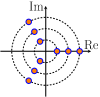
(a)

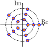
(b)

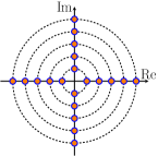
(c)

Figure 2: Three star QAM constellations: (a) $(3,3)$-SQAM, (b) $(3,5)$-SQAM, and (c) $(5,4)$-SQAM.

III-C A Trellis for SQAM Constellations

In this subsection, we provide a trellis diagram, $\mathbb{T}$, that describes the signatures of SLD sequences of length $n$ drawn from $\mathcal{K}_{\mathcal{D},n_{p}}$, an $(n_{r},n_{p})$-SQAM constellation with radius set $\mathcal{D}=\{d_{1},\ldots,d_{n_{r}}\}$. The trellis $\mathbb{T}$ will be used both to design a codebook $\mathcal{S}$ and for decoding.

The length of $\mathbb{T}$ is $2n-1$. The vertex set of $\mathbb{T}$ is given as $\mathcal{V}=\{v_{r}\}\cup\mathcal{V}_{1}\cup\mathcal{V}_{2}\cup\ldots\cup\mathcal{V}_{2n-2}\cup\{v_{g}\},$ where, for $j\in\llbracket{1},{2n-2}\rrbracket$, $\mathcal{V}_{j}$ is the $n_{r}$-set $\mathcal{V}_{j}=\{v_{j}^{1},v_{j}^{2},\ldots,v_{j}^{n_{r}}\}$. Thus, except at depth $0$ and at depth $|\mathbb{T}|$, the trellis $\mathbb{T}$ has exactly $n_{r}$ vertices at each depth. To define the edge-label alphabet of $\mathbb{T}$, for any (not necessarily distinct) $j$ and $k\in\llbracket{1},{n_{r}}\rrbracket$ let

$$\Psi_{j,k}=\{\psi(a,b)\colon a\in\mathcal{D}_{j},~{}b\in\mathcal{D}_{k}\}.$$ (13)

By symmetry, $\Psi_{j,k}=\Psi_{k,j}$. Let $\mathcal{A}_{\text{ISI-present}}=\bigcup_{j=1}^{n_{r}}\bigcup_{k=1}^{n_{r}}\Psi_{j,k}$ and let $\mathcal{A}_{\text{ISI-free}}=\{d_{1}^{2},\ldots,d_{n_{r}}^{2}\}$. The edge-label alphabet of $\mathbb{T}$ is then given as $\mathcal{A}=\mathcal{A}_{\text{ISI-present}}\cup\mathcal{A}_{\text{ISI-free}}$.

Finally, to define the edge set of $\mathbb{T}$, let

$$\mathcal{E}_{r} =\left\{(v_{r},d_{j}^{2},v_{1}^{j}):j\in\llbracket{1},{n_{r}}\rrbracket\right\},$$

$$\mathcal{E}_{g} =\left\{(v_{2n-2}^{j},d_{j}^{2},v_{g}):j\in\llbracket{1},{n_{r}}\rrbracket\right\},$$

$$\mathcal{E}_{\text{ISI-present}} =\Big{\{}(v_{2b+1}^{j},\zeta,v_{2b+2}^{k}):b\in\llbracket{0},{n-2}\rrbracket,$$

$$\quad\quad j,k\in\llbracket{1},{n_{r}}\rrbracket,\zeta\in\Psi_{j,k}\Big{\}},$$

$$\mathcal{E}_{\text{ISI-free}} =\Big{\{}(v_{2b}^{j},d_{j}^{2},v_{2b+1}^{j}):b\in\llbracket{1},{n-2}\rrbracket,j\in\llbracket{1},{n_{r}}\rrbracket\Big{\}};$$

then $\mathcal{E}=\mathcal{E}_{r}\cup\mathcal{E}_{g}\cup\mathcal{E}_{\text{ISI-present}}\cup\mathcal{E}_{\text{ISI-free}}$. Note that $\mathcal{E}_{r}$ is the set of edges in $\mathbb{T}$ incident from the root vertex $v_{r}$, $\mathcal{E}_{g}$ is the set of edges incident to the goal vertex $v_{g}$, $\mathcal{E}_{\text{ISI-present}}$ are edges incident from vertices at odd depth, while $\mathcal{E}_{\text{ISI-free}}$ are edges incident from vertices at even depth. There are $|\Psi_{j,k}|$ parallel edges between $v_{2b+1}^{j}$ and $v_{2b+2}^{k}$, for $b\in\llbracket{0},{n-2}\rrbracket$ and $j,k\in\llbracket{1},{n_{r}}\rrbracket$.

Example 1.

In this example, we sketch the trellis diagram for the $(3,3)$-SQAM constellation with radius set $\mathcal{D}=\{2\sqrt{2},4\sqrt{2},6\sqrt{2}\}$, as shown in Fig. 2a, when the length of SLD sequences is $n=3$. We have $\Psi_{1,1}=\left\{8,5\right\}$, $\Psi_{1,2}=\left\{19,13\right\}$, $\Psi_{1,3}=\left\{27,36\right\}$, $\Psi_{2,2}=\left\{20,32\right\}$, $\Psi_{2,3}=\left\{33,51\right\}$, and $\Psi_{3,3}=\left\{45,72\right\}$. The resulting trellis is shown in Fig. 3. One may see that for $b\in\{1,3\}$, the edge labels between, for example, $v_{b}^{1}$ and $v_{b+1}^{3}$ belong to $\Psi_{1,3}$. Similarly, the edge label between, for example, $v_{2}^{2}$ to $v_{3}^{2}$ is equal to $(4\sqrt{2})^{2}$. For ease of reading, the radius set $\mathcal{D}$ for this example was judiciously chosen to result in integer edge labels.

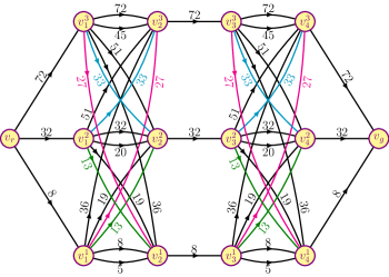
Figure 3: The trellis for Example 1.

Theorem 1 gives the number of parallel edges between $v_{j}^{k}$ and $v_{j+1}^{\ell}$, for an odd $j\in\{1,3,\ldots,2n-1\}$.

Theorem 1.

For any $k$ and $\ell\in\llbracket{1},{n_{r}}\rrbracket$, $|\Psi_{k,\ell}|=\lceil\frac{n_{p}+1}{2}\rceil$.

Proof:

The phase difference between any $a\in\mathcal{D}_{k}$ and $b\in\mathcal{D}_{\ell}$ is in $\Phi_{n_{p}}$ and, since $\cos(\theta)=\cos(2\pi-\theta)$, for any $\theta\in\mathbb{R}$, we leave it to the reader to check that there are exactly $\lceil\frac{n_{p}+1}{2}\rceil$ distinct values for $\cos(\arg(ab^{\ast}))$. ∎

For example, Fig. 4 illustrates the situation that arises when $n_{p}=8$ and $n_{p}=9$, for which $|\Psi_{k,\ell}|=5$.

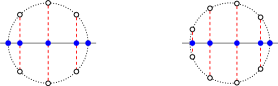
Figure 4: Illustrating Theorem 1. The filled circles show the possible values for $\cos(\arg(ab^{\ast}))$.

The following theorem counts $|\mathcal{P}_{\mathbb{T}}|$, the number of distinct directed paths from root to goal in $\mathbb{T}$.

Theorem 2.

For the trellis $\mathbb{T}$ of length $2n-1$ described in Sec. III-C,

$$|\mathcal{P}_{\mathbb{T}}|=\left\lceil\frac{n_{p}+1}{2}\right\rceil^{n-1}n_{r}^{n}.$$

Proof:

Let $\bm{A}_{j}$ denote the adjacency matrix of the $j$th trellis section of $\mathbb{T}$. We have

$$\bm{A}_{j}=\begin{cases}\mathds{1}_{1\times n_{r}},&j=0,\\ \bm{I}_{n_{r}},&j\in\{2,4,\ldots,2n-4\},\\ \left\lceil\frac{n_{p}+1}{2}\right\rceil\mathds{1}_{n_{r}\times n_{r}},&j\in\{1,3,\ldots,2n-3\},\\ \mathds{1}_{n_{r}\times 1},&j=2n-2,\end{cases}$$

where the case for odd $j$ follows from Theorem 1. The number of paths from root to goal in $\mathbb{T}$ is then given as

$$|\mathcal{P}_{\mathbb{T}}|=\prod_{j=0}^{2(n-1)}\bm{A}_{j}=\left\lceil\frac{n_{p}+1}{2}\right\rceil^{n-1}n_{r}^{n}.$$

∎

The next theorem shows that there is a one-to-one correspondence between $\mathcal{P}_{\mathbb{T}}$ and $\mathcal{L}_{\mathbb{T}}$.

Theorem 3.

$|\mathcal{P}_{\mathbb{T}}|=|\mathcal{L}_{\mathbb{T}}|$.

Proof:

The map $\lambda$ taking paths in $\mathcal{P}_{\mathbb{T}}$ to label sequences in $\mathcal{L}_{\mathbb{T}}$ is surjective by definition. For $\lambda$ to be injective, every label sequence $(\ell_{0},\ell_{1},\ldots,\ell_{2n-2})\in\mathcal{L}_{\mathbb{T}}$ must have a unique pre-image $\bm{p}\in\mathcal{P}_{\mathbb{T}}$. The set of vertices through which $\bm{p}$ traverses is uniquely determined by $(\ell_{0},\ell_{2},\ldots,\ell_{2n-2})$. Furthermore, the selection from among parallel edges in the odd trellis sections is uniquely determined by $(\ell_{1},\ell_{3},\ldots,\ell_{2n-3})$, since such parallel edges have distinct labels. ∎

III-D Finding Square-law Distinct Sequences Using the Trellis

Finding SLD sequences for a relatively small constellation size and a small block length $n$ is feasible by computer search. For example, for a constellation $\mathcal{K}$, one may produce two matrices, $\mathcal{Q}\in\mathcal{K}^{|\mathcal{K}|^{n}\times n}$ and $\mathcal{M}\in\mathbb{R}^{|\mathcal{K}|^{n}\times(2n-1)}$ where the rows of $\mathcal{Q}$ are all possible $n$-vectors defined over $\mathcal{K}$ and the rows of $\mathcal{M}$ are the corresponding signatures. Then, one may find all SLD sequences (which are some rows of $\mathcal{Q}$) by deleting the duplicated rows of $\mathcal{M}$.

For large values of constellation size or block length $n$, finding those sequences by exhaustive search is computationally intractable. Fortunately, SLD sequences drawn from an $(n_{r},n_{p})$-SQAM constellation can be found using the trellis described in Sec. III-C.

Recall that two $n$-tuples $\bm{s}$ and $\tilde{\bm{s}}$ in $\mathcal{K}_{\mathcal{D},n_{p}}^{n}$ are square-law equivalent, written $\bm{s}\equiv\tilde{\bm{s}}$, if $\Upsilon(\bm{s})=\Upsilon(\tilde{\bm{s}})$, i.e., if the two $n$-tuples have the same signature. The set of such $n$-tuples is partitioned into disjoint equivalence classes. A transversal of this collection of classes is then any subset $\mathcal{T}\subset\mathcal{K}_{\mathcal{D},n_{p}}^{n}$ containing exactly one element from each equivalence class. We call such a transversal an SLD-transversal since, by definition, the elements of any such transversal are SLD. A codebook $\mathcal{S}$ is, by definition, a subset of an SLD-transversal; therefore, SLD-transversals are the largest possible codebooks that can be used for the system described in Sec. II.

Theorem 4.

For every SLD-transversal $\mathcal{T}$,

$$\{\Upsilon(\bm{s})\colon\bm{s}\in\mathcal{T}\}=\mathcal{L}_{\mathbb{T}}.$$

In other words, the signature of each $n$-vector in an SLD-transversal is a label sequence in $\mathcal{L}_{\mathbb{T}}$, and each label sequence in $\mathcal{L}_{\mathbb{T}}$ is the signature of an $n$-vector in the SLD-transversal.

Proof:

This follows from the definitions of $\mathcal{A}_{\text{ISI-free}}$ and $\mathcal{A}_{\text{ISI-present}}$ and Theorem 3. ∎

Corollary 4.1.

The maximum rate that can be achieved by an $(n_{r},n_{p})$-SQAM constellation with the system described in Sec. II, as $n\rightarrow\infty$, is $\log_{2}\left(n_{r}\left\lceil\frac{n_{p}+1}{2}\right\rceil\right)$ b/sym.

Proof.

This follows Theorems 2, 3, and 4. ∎

Note that the maximum achievable rate for an $(n_{r},n_{p})$-SQAM constellation under coherent detection is $\log_{2}\left(n_{r}n_{p}\right)$ and

$$0<\log_{2}\left(n_{r}n_{p}\right)-\log_{2}\left(n_{r}\left\lceil\frac{n_{p}+1}{2}\right\rceil\right)<1.$$

According to Theorem 4, SLD-transversals are all mapped to the set $\mathcal{L}_{\mathbb{T}}$ by the function $\Upsilon$. Thus every SLD-transversal is equivalent from the perspective of the detector, i.e., all of SLD-transversals will have the same error rate. In the following, we describe an algorithm that uses the trellis $\mathbb{T}$ to determine a particular SLD-transversal.

An $n$-vector $(s_{0},\ldots,s_{n-1})\in\mathcal{K}_{\mathcal{D},n_{p}}^{n}$ is called standard if

1. $s_{0}\in\mathbb{R}^{>0}$, and

2. $\arg(s_{\ell+1}s_{\ell}^{\ast})\in[0,\pi],\text{ for every }\ell\in\llbracket{0},{n-2}\rrbracket$.

In other words, the first component of a standard vector is a positive real number, and the argument of each component is obtained from the argument of the previous component by adding (modulo $2\pi)$ an angle in the range $[0,\pi]$.

Define a family of functions

$$\varphi(\cdot;a,b)\colon\left[\frac{3}{8}(a^{2}+b^{2})-\frac{ab}{4},\frac{3}{8}(a^{2}+b^{2})+\frac{ab}{4}\right]\to[0,\pi],$$

indexed by positive real numbers $a$ and $b$, and given as

$$\varphi(\zeta;a,b)=\arccos\left(\frac{8\zeta-3(a^{2}+b^{2})}{2ab}\right).$$

Given two complex numbers $z_{a}$ and $z_{b}$ such that $|z_{a}|=a$, $|z_{b}|=b$, and $\psi(z_{a},z_{b})=\zeta$, there are at most two possible values of $\arg(z_{a}z_{b}^{\ast})$, namely $\varphi(\zeta;a,b)\in[0,\pi]$ and $2\pi-\varphi(\zeta;a,b)\in[\pi,2\pi]$. The function $\varphi(\cdot;a,b)$ is defined to select the first of these possibilities.

Theorem 5.

Each equivalence class (under square-law equivalence) $\mathcal{C}\subset\mathcal{K}_{\mathcal{D},n_{p}}^{n}$ contains exactly one standard vector.

Proof:

The signature of each vector in $\mathcal{C}$ is the same, given as, say, $\bm{\zeta}=(\zeta_{0},\ldots,\zeta_{2n-2})\in\mathbb{R}^{2n-1}$. Let

$$s_{0}=\sqrt{\zeta_{0}},$$ (14)

and, for $\ell\in\llbracket{0},{n-2}\rrbracket$, let

$$s_{\ell+1}=\frac{\sqrt{\zeta_{2\ell}\zeta_{2\ell+2}}}{s^{\ast}_{\ell}}\exp\left(i\varphi\left(\zeta_{2\ell+1};\sqrt{\zeta_{2\ell}},\sqrt{\zeta_{2\ell+2}}\right)\right).$$ (15)

Let $\bm{s}=(s_{0},\ldots,s_{n-1})$. From (14) and $(\ref{eq:s2})$ we have $\Upsilon(\bm{s})=\bm{\zeta}$; thus, $\bm{s}\in\mathcal{C}$. Furthermore, by construction, $\bm{s}$ is standard. Uniqueness follows from the fact that the function $\varphi$ always chooses (from two possibilities) the unique phase difference between successive components that results in a standard vector. ∎

Define $\Upsilon^{-1}:\mathcal{L}_{\mathbb{T}}\to\mathcal{T}_{\text{s}}$ that, given a signature $(\zeta_{0},\ldots,\zeta_{2n-2})\in\mathcal{L}_{\mathbb{T}}$ returns the standard vector with that signature, as determined by (14) and (15).

The (unique) SLD-transversal containing only standard vectors, denoted by $\mathcal{T}_{\text{s}}$, is called the standard SLD-transversal. The elements of $\mathcal{T}_{\text{s}}$ can be computed by applying $\Upsilon^{-1}$ to the label sequences obtained by following every possible path from root to goal in the trellis $\mathbb{T}$. When $|\mathcal{T}_{\text{s}}|$ is sufficiently small, the elements of $\mathcal{T}_{\text{s}}$ be stored in a lookup table, thereby allowing for an efficient mapping between messages and codewords. This is the approach followed for the codebooks $\mathcal{S}$ studied in this paper, which are obtained as power-of-two subsets of $\mathcal{T}_{\text{s}}$.

For larger codebooks, the mapping between messages and codewords becomes more complicated, possibly requiring enumerative encoding techniques to select a suitable path through $\mathbb{T}$. However, once such a path is selected, computation of a standard vector is readily accomplished by applying $\Upsilon^{-1}$ to the corresponding label sequence.

III-E Trellis Decoding

In addition to determining $\mathcal{T}_{\text{s}}$, the trellis $\mathbb{T}$ of Sec. III-C can be used with the Viterbi algorithm to detect the sequence $\hat{\bm{x}}\in\mathcal{S}$ from the noisy received vectors $\bm{y}=(y_{0},\ldots,y_{n-1})$ and $\bm{z}=(z_{0},\ldots,z_{n-2})$. For the reasons of simplicity noted in Sec. II-F, we use (11) and (12) in branch-metric computation to approximate true ML detection.

Consider the transmission of the standard vector corresponding to the label sequence associated with some trellis path $\bm{p}=(e_{0},\ldots,e_{2n-2})\in\mathcal{P}_{\mathbb{T}}$. From (5), (6), (9), (10), and Theorem 4 one may see that, in the absence of noise, the received values are (to a close approximation) a scaled version of the edge labels. In particular, in the noise-free case, $y_{k}\simeq\mathfrak{R}\,\beta e^{-\varrho L}\left(E_{\text{in}}\kappa\alpha_{\beta}\right)^{2}\lambda(e_{2k})$ and $z_{\ell}\simeq\mathfrak{R}\,(1-\beta)e^{-\varrho L}\left(E_{\text{in}}\kappa\alpha_{\beta}\right)^{2}\lambda(e_{2\ell+1})$, for any $k\in\llbracket{0},{n-1}\rrbracket$ and $\ell\in\llbracket{0},{n-2}\rrbracket$.

Now in the presence of noise, from (11) and (12) it follows that the mean and the variance of the received $\bm{y}$ and $\bm{z}$ entries are, respectively, linear and affine functions of the entries of the label sequence $\lambda(\bm{p})$ in our approximation. In particular, for any edge $e\in\mathcal{E}$, let $\mathsf{Mean}:\mathcal{E}\rightarrow\mathbb{R}$, and $\mathsf{Var}:\mathcal{E}\rightarrow\mathbb{R}$ be defined as

$$\mathsf{Mean}(e)=\mathfrak{R}\,e^{-\varrho L}\left(E_{\text{in}}\kappa\alpha_{\beta}\right)^{2}\lambda(e),$$

and

$$\mathsf{Var}(e)=e^{-\varrho L}\left(E_{\text{in}}\kappa\alpha_{\beta}\right)^{2}\sigma_{\text{sh}}^{2}\lambda(e)+T\sigma_{\text{th}}^{2}.$$

Thus for an edge $e_{2j}$ in the $(2j$)th trellis section, $j\in\llbracket{0},{n-1}\rrbracket$, incident from a vertex of even depth, the mean and the variance of $y_{j}$ are given as $(1-\beta)\mathsf{Mean}(e_{2j})$ and $(1-\beta)\mathsf{Var}(e_{2j})$, respectively. Similarly for an edge $e_{2j+1}$ in the $(2j+1)$th trellis section, $j\in\llbracket{0},{n-2}\rrbracket$, incident from a vertex of odd depth, the mean and the variance of $z_{j}$ are given as $\beta\mathsf{Mean}(e_{2j+1})$ and $\beta\mathsf{Var}(e_{2j+1})$, respectively.

We define two branch-metric functions, $w_{\text{ISI-free}}:\mathbb{R}\times\mathcal{E}\rightarrow\mathbb{R}$, and $w_{\text{ISI-present}}:\mathbb{R}\times\mathcal{E}\rightarrow\mathbb{R}$, as follows. Let

$$w_{\text{ISI-free}}(y,e)=\frac{\big{(}y-(1-\beta)\mathsf{Mean}(e)\big{)}^{2}}{(1-\beta)\mathsf{Var}(e)}+\ln\left(\mathsf{Var}(e)\right),$$

and let

$$w_{\text{ISI-present}}(z,e)=\frac{\big{(}z-\beta\mathsf{Mean}(e)\big{)}^{2}}{\beta\mathsf{Var}(e)}+\ln\left(\mathsf{Var}(e)\right),$$

for any $y$ and $z\in\mathbb{R}$ and any $e\in\mathcal{E}$.

To detect $\hat{\bm{x}}$ from $\bm{y}$ and $\bm{z}$, one may run the Viterbi algorithm on $\mathbb{T}$ with branch metrics defined above to determine the path $\bm{p}_{\text{mw}}\in\mathcal{P}_{\mathbb{T}}$ of minimum total weight, computing

$$\bm{p}_{\text{mw}}=\underset{(e_{0},\ldots,e_{2n-2})\in\mathcal{P}_{\mathbb{T}}}{\arg\min}\\ \sum_{j\in\llbracket{0},{n-1}\rrbracket}w_{\text{ISI-free}}(y_{j},e_{2j})+\sum_{j\in\llbracket{0},{n-2}\rrbracket}w_{\text{ISI-present}}(z_{j},e_{2j+1}).$$

The detected codeword is then $\hat{\bm{x}}=\Upsilon^{-1}(\lambda(\bm{p}_{\text{mw}}))$, provided that $\hat{\bm{x}}\in\mathcal{S}$. In case $\hat{\bm{x}}\not\in\mathcal{S}$, a decoding failure is declared. In practice, $\mathcal{S}$ is selected to have as many codewords from $\mathcal{T}_{\text{s}}$ as possible, while still having a size that is a power of two. Thus the majority of paths in $\mathcal{P}_{\mathbb{T}}$ are codewords, and decoding failures are rare. Indeed, the numerical simulations of Sec. IV do indeed confirm that, at the launch powers required to achieve reasonably small decoding error rates, the probability of decoding failure is negligible.

IV Numerical Simulation

In this section, the schemes described in sections II and III are verified by numerical simulations.

IV-A Simulation Setup

Because we consider square-law detection with both shot noise and thermal noise, a notion of signal-to-noise ratio (SNR), as would be appropriate for linear additive white Gaussian channels, is not appropriate here. Accordingly, the various figures of merit considered here are shown as functions of launch power. We use practical values for $\sigma_{\text{sh}}^{2}$ and $\sigma_{\text{th}}^{2}$ in all cases.

In all simulations we have assumed a transmission length of $L=10~{}\text{km}$. Furthermore, laser power refers to the mean-squared power of the unmodulated waveform, i.e., $\frac{1}{2}E_{\text{in}}^{2}$.

In [1] it is shown that $\beta=0.9$ provides near-optimal error rates and achievable rate performance versus launch power. However, $\beta=0.9$ requires integration intervals as short as $10\%$ of a symbol period, which may be difficult to implement at high symbol rates. To tackle this issue, we have used $\beta=0.5$ in all simulations of this paper, corresponding to an integration period that is $50\%$ of the symbol period for both the ISI-free and ISI-present signalling segments.

The practical ease of $\beta=0.5$ comes at the expense of a worse error rate and a larger bandwidth. Note that Tukey waveforms are time-limited, thus, band-unlimited. Therefore, the typical notion of bandwidth for time-limited waveforms, e.g., sinc and raised-cosine waveforms, does not apply to Tukey waveforms. For this reason, we use $95\%$ in-band-energy as the bandwidth criterion for comparing Tukey waveforms with each other. While $w_{0.9}(\cdot)$ has a $15\%$ spectral overhead compared to the minimum required bandwidth for Nyquist signalling, the spectral overhead of $w_{0.5}(\cdot)$ is $33.6\%$. However, spectral efficiency may not be an important performance criterion in some applications, e.g., in data-center interconnects, and so the spectral overhead of Tukey waveforms may not be an important concern in such applications.

IV-B The Photodiode

The simulations in this chapter are done by assuming the use of an InGaAs p-i-n photodiode at the receiver. This choice gave better performance than avalanche photodiodes in our simulations. The reason for its better performance is that, as explained in Sec. II-F, the performance of direct detection schemes depends on the symbol rate and at sufficiently large symbol rates shot noise dominates thermal noise. As noted by Agrawal, “the SNR of APD receivers is worse than that of p-i-n receivers when shot noise contribution is concerned.” [16].

The two-sided power spectral density of the thermal noise is [16]

$$\sigma_{\text{th}}^{2}=\frac{2\mathsf{k}T_{k}}{R_{L}},$$

where $\mathsf{k}$ is the Boltzmann constant, $T_{k}$ is the absolute temperature, and $R_{L}$ is the load resistor. In the simulations we have used $T_{k}=300$ K and $R_{L}=300~{}\Omega$. Furthermore, the two-sided power spectral density of $n_{\text{sh}}(t)$ of a p-i-n photodiode is $\sigma_{\text{sh}}^{2}=\mathsf{e}\mathfrak{R}$, where $\mathsf{e}$ is the elementary charge [16]. The typical range for the responsivity of an InGaAs p-i-n photodiode is $0.6-0.9~{}\text{mA/mW}$ [16]; in the simulations, we have used $\mathfrak{R}=0.75~{}\text{mA/mW}$.

IV-C Codebook-size Constraint

In all of our numerical simulations, we have assumed that $|\mathcal{S}|=M$ is a power of two. For example, for the $(8,4)$-SQAM constellation and with a block length of $5$, we have chosen $2^{21}=2097152$ of the $\left|\mathcal{T}_{\text{s}}\right|=2654208$ available SLD sequences to form $\mathcal{S}$. Under this power-of-two restriction, the maximum achievable rate of the proposed scheme using $(n_{r},n_{p})$-SQAM with a block length $n$ is

$$\frac{1}{n}\left\lfloor\log_{2}\left(\left\lceil\frac{n_{p}+1}{2}\right\rceil^{n-1}n_{r}^{n}\right)\right\rfloor\quad\text{b/sym}.$$

IV-D Optimizing Ring Spacing

A pair of $n_{r}$ and $n_{p}\in\mathbb{Z}^{\geq 2}$ does not uniquely specify an $(n_{r},n_{p})$-SQAM constellation; one must also specify the radius set $\mathcal{D}$. In this section, for a fixed $n_{r}$ and $n_{p}$ we try to find the best value of $\delta\in\mathbb{R}^{>0}$ such that

$$\mathcal{D}=\left\{1,1+\delta,1+2\delta,\ldots,1+(n_{r}-1)\delta\right\}.$$ (16)

Fig. 5 shows the BER of $(8,4)$-SQAM constellations for different values of $\delta$. For these constellations $M=|\mathcal{S}|=2^{12}$ and $n=3$; thus, their maximum achievable rate is $4$ b/sym. One can see that among the tested $\delta$ values, $\delta=0.2$ has the best performance.

Table I shows the best $\delta$ for different constellations. The tested values of $\delta$ are similar to those of Fig. 5. The criteria for choosing the best $\delta$ is the one which results in the least launch power at BER of $10^{-3}$. The rows which are not highlighted are those for which we can achieve at least as great a rate, in b/sym, with another $(n_{r},n_{p})$-SQAM constellation at the same symbol rate, yet with smaller launch power. For example, the row of $(2,5)$-SQAM constellation is not highlighted as at $50$ Gbaud it achieves a rate of about $2.2$ b/sym at a launch power of $-9$ dBm while $(3,2)$-SQAM constellation achieves $2.43$ b/sym at a launch power of $-12.2$ dBm. Thus, we are interested only in highlighted rows.

Theorem 2 implies that the maximum codebook size, $|\mathcal{T}_{\text{s}}|$, depends on $\left\lceil\frac{n_{p}+1}{2}\right\rceil$. As a result, for a fixed block length $n$ and a radius set $\mathcal{D}$, an $(n_{r},n_{p})$-SQAM constellation with an even $n_{p}$ results in the same transversal cardinality as an $(n_{r},n_{p}+1)$-SQAM constellation. Therefore, as the ring points of the former constellation are further apart than those of the latter one, we expect the $(n_{r},n_{p})$-SQAM constellation to have a better performance than the $(n_{r},n_{p}+1)$ constellation. Table I does indeed support this claim, as all highlighted rows have an even $n_{p}$.

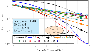
Figure 5: BER curves for several $(8,4)$-SQAM constellations with $n=3$.

IV-E Bit Error Rate

Fig. 6 shows the trellis decoding bit error rate of the proposed scheme for the constellations highlighted in Table I at $50~{}$Gbaud and with $1~{}$dBm laser power. As it is apparent, the BER curves have two parts: 1) a roll-down part where the BER decreases with a higher launch power, and 2) a roll-up part which behaves in the opposite manner. The reason for the roll-up part is that the proposed decoder approximates the transmitted waveform as (4), while the waveform actually suffers from nonlinear distortion according to (1). As mentioned in II-F, this is a good approximation when the power of the modulating waveform, $u(t)$, is relatively small. For a fixed laser power, the launch power is controlled by the modulating-waveform power; i.e., a high launch-power demands a higher modulating-waveform power which degrades the accuracy of approximating (1) with (4).

Fortunately, a practical raw BER, e.g., about $10^{-3}$, can be achieved in the roll-down area for all considered constellations, except $(12,4)$-, $(13,4)$-, and $(16,4)$-SQAM constellations. This is the reason that some cells corresponding to those particular constellations in Table I are left blank. For example, the smallest BER obtained by a $(16,4)$-SQAM constellation at $50$ Gbaud is about $0.011$, is achieved at a launch power about $-7.9~{}$dBm and with $\delta=0.2$.

As explained in section III-E, the power-of-two constraint may cause the trellis decoder to declare a decoding failure. Fig. 7 shows the decoding failure probability for the same constellations as Fig. 6. The constellations which are absent in Fig. 7 but are present in Fig. 6 had no decoding failure at the tested launch power values. By comparing Fig. 7 with 6 one may see that at launch power values with a practically small BER, e.g., $10^{-3}$, the decoding failure rate is negligible.

As noted in Sec. II-F, unlike a typical AWGN communication scheme, the performance under direct detection depends on the symbol rate. This fact is illustrated in Fig. 8 which provides the BER curves in the same setup as Fig. 6, except that it is at $25$ Gbaud. By comparing these two figures one may see that for a fixed constellation, a BER of $10^{-3}$ can be achieved with approximately $1.5~{}$dB less launch power at $25~{}$Gbaud than at $50~{}$Gbaud.

Note that in computing BER we treat decoding failures as equivalent to a momentary BER of $0.5$. We made no attempt to optimize (e.g., by Gray labelling) the mapping of sequences $\bm{x}\in\mathcal{S}$ to binary vectors of length $\log_{2}(|\mathcal{S}|)$.

TABLE I: Optimal ring spacing for different star-QAM constellations.

$\bm{(n_{r},n_{p})}$	$\bm{n}$	max rate (b/sym)	launch power (dBm) at 50 Gbaud	launch power (dBm) at 25 Gbaud	optimal $\bm{\delta}$
$(2,3)$	$5$	$1.8$	$-12.6$	$14.1$	$0.2$
$(2,2)$	$7$	$1.86$	$-13.25$	$-14.75$	$0.2$
$(2,4)$	$4$	$2$	$-10.6$	$-12$	$0.2$
$(2,5)$	$5$	$2.2$	$-9$	$-10.5$	$0.2$
$(3,3)$	$4$	$2.25$	$-12.1$	$-13.5$	$0.2$
$(3,2)$	$7$	$2.43$	$-12.2$	$-13.6$	$0.2$
$(2,6)$	$4$	$2.5$	$-8.2$	$-9.7$	$0.1$
$(4,3)$	$4$	$2.75$	$-11.8$	$-13.3$	$0.2$
$(3,5)$	$4$	$2.75$	$-9$	$-10.4$	$0.1$
$(3,4)$	$4$	$2.75$	$-10.3$	$-11.8$	$0.2$
$(4,2)$	$6$	$2.83$	$-12.2$	$-13.6$	$0.2$
$(5,2)$	$5$	$3$	$-11.2$	$-12.7$	$0.2$
$(5,3)$	$4$	$3$	$-11$	$-12.5$	$0.2$
$(6,3)$	$3$	$3$	$-10.9$	$-12.3$	$0.2$
$(4,4)$	$4$	$3$	$-10$	$-11.6$	$0.2$
$(4,5)$	$3$	$3$	$-8.8$	$-10.3$	$0.1$
$(3,6)$	$4$	$3$	$-8.2$	$-9.7$	$0.1$
$(6,2)$	$5$	$3.2$	$-10.8$	$-12.3$	$0.2$
$(7,2)$	$3$	$3.33$	$-10.3$	$-11.7$	$0.2$
$(7,3)$	$3$	$3.33$	$-10.2$	$-11.6$	$0.2$
$(5,4)$	$3$	$3.33$	$-9.8$	$-11.3$	$0.2$
$(6,4)$	$3$	$3.33$	$-9.7$	$-11.1$	$0.2$
$(5,5)$	$3$	$3.33$	$-8.6$	$-9.9$	$0.1$
$(6,5)$	$3$	$3.33$	$-8.4$	$-9.8$	$0.1$

$\bm{(n_{r},n_{p})}$	$\bm{n}$	max rate (b/sym)	launch power (dBm) at 50 Gbaud	launch power (dBm) at 25 Gbaud	optimal $\bm{\delta}$
$(4,6)$	$3$	$3.33$	$-8$	$-9.7$	$0.1$
$(5,6)$	$3$	$3.33$	$-8$	$-9.6$	$0.1$
$(7,2)$	$5$	$3.6$	$-10$	$-11.5$	$0.2$
$(9,3)$	$3$	$3.67$	$-9.3$	$-10.8$	$0.2$
$(8,3)$	$3$	$3.67$	$-9.9$	$-11.4$	$0.2$
$(10,3)$	$3$	$3.67$	$-9.1$	$-10.6$	$0.2$
$(7,5)$	$3$	$3.67$	$-8.1$	$-9.4$	$0.1$
$(7,4)$	$3$	$3.67$	$-9.3$	$-10.8$	$0.2$
$(8,2)$	$5$	$3.8$	$-10.2$	$-11.7$	$0.2$
$(8,3)$	$5$	$3.8$	$-9.9$	$-11.4$	$0.2$
$(8,4)$	$3$	$4$	$-8.8$	$-10.3$	$0.2$
$(11,3)$	$3$	$4$	$-8.5$	$-9.9$	$0.2$
$(9,4)$	$3$	$4$	$-8.6$	$-10.1$	$0.2$
$(12,3)$	$3$	$4$	$-8.5$	$-9.9$	$0.2$
$(9,5)$	$3$	$4$	$-7.6$	$-8.9$	$0.1$
$(8,5)$	$3$	$4$	$-7.9$	$-9.3$	$0.1$
$(7,6)$	$3$	$4$	$-7.7$	$-9.2$	$0.1$
$(8,4)$	$5$	$4.2$	$-8.4$	$-9.9$	$0.2$
$(10,4)$	$3$	$4.33$	$-8$	$-9.5$	$0.2$
$(11,4)$	$3$	$4.33$	$-8$	$-9.5$	$0.2$
$(12,4)$	$3$	$4.33$	—	$-9.2$	$0.2$
$(8,6)$	$3$	$4.33$	$-7.4$	$-9$	$0.1$
$(13,4)$	$3$	$4.67$	—	$-8.6$	$0.2$
$(16,4)$	$3$	$5$	—	—	$0.2$

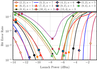
Figure 6: BER curves for the constellations highlighted in Table I at $50$ Gbaud and with $1~{}$dBm laser power.

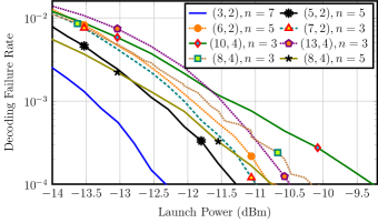
Figure 7: Decoding failure rate for the constellations highlighted in Table I, at $50$ Gbaud and with $1~{}$dBm laser power. The constellations that are not present in this figure had no decoding failure at the tried launch powers.

IV-F Achievable Data Rate

Fig. 9 shows the theoretically maximum achievable data rate for a few SQAM constellations at $50$ Gbaud and with a $1$ dBm laser power, obtained by Monte Carlo simulations. Except the $(16,4)$-SQAM constellation with block length $n=3$, the remaining constellations are chosen from the ones highlighted in Table I but possibly with a different block length $n$. For the $(16,4)$-SQAM constellation we have $\delta=0.2$ in (16).

Similar to the BER figures, the rate figures are obtained by the power-of-two constraint on $|\mathcal{S}|$. Without this constraint, the maximum achievable rate of each constellation can be increased up to $\frac{1}{n}$ bits. For example, for the $(5,2)$-SQAM constellation with $n=4$, the maximum achievable rate by using all SLD sequences is $\log_{2}|\mathcal{T}_{\text{s}}|\simeq 3.07$ b/sym. However, as only $2^{12}=4096$ symbols have been chosen out of $5000$ SLD sequences, the rate has decreased to $3$ b/sym.

Fig. 9 shows the necessity of using error correcting codes from two perspectives. First, a desired rate can be achieved using a higher-order constellation along with an error correcting code at a lower launch power. For example, while the uncoded $(8,4)$-SQAM constellation with $n=3$ can achieve $4$ b/sym at a launch power of $-9.5$ dBm, the same rate can be achieved with a $(10,4)$-SQAM constellation with $n=3$ and an error correcting code of rate $\frac{12}{13}$ at a launch power of $-12$ dBm; resulting in a coding gain of about $2.5$ dBm. Secondly, at a fixed launch power, a higher data rate can be achieved by using a higher-order constellation along with an error correcting code. For example, at a launch power of $-12$ dBm, the uncoded $(5,2)$-SQAM constellation with $n=4$ can achieve a rate of $3$ b/sym, while by using the $(8,4)$ constellation with $n=3$ along with an error correcting code of rate $\frac{15}{16}$ one may achieve $3.75$ b/sym.

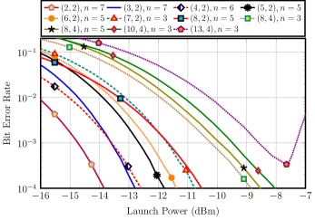
Figure 8: BER curves for the constellations highlighted in Table I at $25$ Gbaud and with $1~{}$dBm laser power.

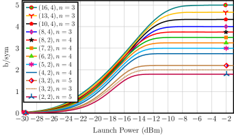
Figure 9: Achievable data rate for different star-QAM constellations. Except $(16,4)$-SQAM constellation, other constellations are highlighted in Table I, but with a possibly different block length. Curves are obtained at $50$ Gbaud and with $1$ dBm laser power.

Another fact which is shown in Fig. 9 is the role of the block length $n$ on the performance. While the maximum achievable rate for the $(3,2)$-SQAM constellation is $2$ b/sym with a block length of $n=3$, it is $2.2$ b/sym with $n=5$. Note that, in contrast to [1], where brute-force search was used, the increase in data rate resulting from a larger $n$ does not come with a huge increase in decoding complexity as the complexity of trellis decoding is linear in $n$.

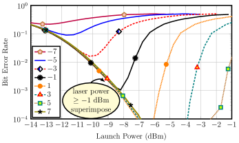
(a)

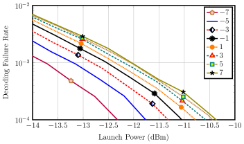
(b)

Figure 10: The BER and decoding failure rate for the $(8,4)$-SQAM constellation with $n=5$, $\delta=0.2$ (see (16)), and at $50~{}$Gbaud, at different laser powers. Legends show the laser power in dBm.

IV-G Effect of Laser Power

Fig. 10a shows the BER of the $(8,4)$-SQAM constellation with $\delta=0.2$, as recommended by Table I, $n=5$, and at $50~{}$Gbaud. Note that the BER curves corresponding to a laser power of $\geq-1~{}$dBm superimpose in the region of interest, i.e., the region with BER about $10^{-3}$. However, the BER performance degrades as laser power drops further. The reason for this behavior is again in approximating (1) with (4). For a fixed launch power, a lower laser power demands a higher modulating-waveform power and it violates the condition for an accurate approximation of (1) by (4).

From Fig. 10a one may conclude that the laser power determines the BER at which the roll-down part of the BER curve meets the roll-up part. In other words, the larger is the laser power, the smaller is the BER at the transition point. For example, while the roll-down to roll-up transition occurs at a BER of about $2\times 10^{-2}$ for a laser power of $-3~{}$dBm, it happens at a BER of $10^{-3}$ and $<10^{-4}$ for a laser power of $-1~{}$dBm and $1~{}$dBm, respectively. Therefore, depending on the minimum required uncoded BER, one may determine the minimum required laser power.

Fig. 10b shows the decoding failure rate with the same simulation setup as in Fig. 10a. Interestingly, in contrast to the BER curves, the smaller is the laser power, the smaller is the decoding failure rate. However, the smaller decoding failure rate comes with a higher bit error rate. From the spacing between the decoding failure rate curves it is apparent that the curves approach a limiting curve as the laser power increases. However, note that launch power values which result a target BER, e.g., about $10^{-3}$, the decoding failure rate is almost negligible.

Fig. 11 shows the BER curves for the $(2,2)$-SQAM constellation with $\delta=0.2$ and block length $n=7$. The maximum achievable rate for this constellation and $n$ is $\frac{13}{7}$ b/sym. By comparing Fig. 10a with Fig. 11 one may see that increasing constellation size, thus rate, increases the minimum required laser power to get a target BER. For example, while we can achieve a BER of $10^{-3}$ with a $-5~{}$dBm or even $-7$ dBm laser power with the described $(2,2)$-SQAM constellation, the minimum required laser power to achieve the same BER with the described $(8,4)$-SQAM constellation is $-1~{}$dBm.

In short-haul applications, e.g., intra data-center communication, power consumed by lasers play are an important component of the overall power budget. One may decide to allocate less power to lasers in the price of a lower data rate, in b/sym, or higher BER for a fixed constellation.

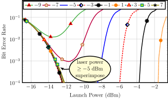
Figure 11: The BER for the $(2,2)$-SQAM constellation with $n=7$ and $\delta=0.2$ (see (16)), and at $50~{}$Gbaud, at different laser powers. Legends show the laser power in dBm.

V Comparing with IMDD

In contrast to the majority of the literature, instead of experimental results all of our figures of merit are obtained by computer-based simulations. There are many practical issues, e.g., splicing, scattering, etc., which have been ignored in our numerical simulations. Therefore, to have a fair comparison, we have simulated IMDD using the same photodiode parameters that were used in our system.

Fig. 12 shows the throughput of the proposed and the IMDD schemes at $50~{}$Gbaud for a single wavelength and a single polarization. While the $(8,4)$-SQAM Tukey signalling achieves a throughput of $200~{}$Gb/s at a launch power of about $-10~{}$dBm, IMDD with PAM-$16$ achieves this rate at about $0~{}$dBm; thus, by using the proposed scheme a again of about $8~{}$dB can be achieved compared to the IMDD scheme. We can achieve the same throughput by using a $(16,4)$-SQAM constellation with $n=3$ and an error correcting code of rate $0.8$ at a launch power about $-12.9~{}$dBm, as well, i.e., a $2.9$ dB coding gain. Furthermore, Fig. 12 shows that for a fixed launch power and a fixed symbol rate one may achieve higher throughputs by using the proposed scheme rather than IMDD. For example, while a throughput of $200$ Gb/s is achievable with the proposed scheme at a launch power of $-10~{}$dBm and at $50~{}$Gbaud with an $(8,4)$-SQAM constellation of block length $n=3$, one may achieve only about $145~{}$Gb/s with an IMDD scheme using PAM-$8$ constellation at the same symbol rate and the same launch power. Note that these two constellations have the same number of magnitude levels; the proposed scheme has a higher throughput since it is able to extract phase information from a complex-valued constellation.

Figure 12: Throughput for IMDD and the proposed scheme at $50~{}$Gbaud.

VI O-band Operation

So far we have assumed operation in the C band according to the system model shown in Fig. 1. Because of the non-negligible chromatic dispersion in this band and the difficulty of post-detection dispersion compensation after signal detection using a single photodiode, dispersion was (partially) precompensated at the transmitter, as discussed in Sec. II-D. However, pre-compensation of chromatic dispersion requires knowledge of the link length, which is generally not possible without a feedback channel.

To remedy this issue, one may operate in the O band, near the zero-dispersion wavelength of SSMF, omitting transmitter-side dispersion precompensation, and making the transmitter agnostic to the transmission distance. This changes the system model to that of Fig. 13. The advantage of having a link-length agnostic transmitter comes at the expense of having channel with greater loss compared to a C-band channel. In particular, the fiber loss in O band is about $0.5~{}\text{dB}\cdot\text{km}^{-1}$.

Fig. 14 shows the O-band BER for the constellations highlighted in Table I, using a laser power of $2~{}\text{dBm}$ and at a symbol rate of $50~{}\text{Gbaud}$. We do not assume operation with exactly zero dispersion; instead we simulate operation at two wavelengths assumed to have chromatic dispersions of $-1$ and $1~{}\text{ps}\cdot\text{nm}^{-1}\cdot\text{km}^{-1}$, respectively, leaving the channel with some uncompensated residual dispersion.

For a $10~{}\text{km}$ length of SSMF, the total power loss of the transmission link in the O band is $3~{}\text{dB}$ more than the total power loss in the C band. We see this by comparing the roll-down parts of the curves in Fig. 14 with their corresponding curves in Fig. 6. For example, one may see from Fig. 14 that the $(8,4)$-SQAM constellation with block length $n=3$ achieves a BER of $10^{-3}$ at a launch power of $-5.8~{}\text{dBm}$ in the O band; while, from Fig. 6, this constellation achieves the same BER at a launch power of $-8.8~{}\text{dB}$ in the C band.

Note that this “$3~{}\text{dB}$ difference” is violated for the $(10,4)$- and $(13,4)$-SQAM constellations. These large constellations achieve a target BER at a higher launch power compared to the other smaller constellations highlighted in Table I. Furthermore, due to the greater loss in the O band, a higher launch power is required to achieve a target BER. However, as explained in Sec. II-F and for a fixed laser power, the higher launch power results in a higher modulator nonlinearity. Thus, it is the nonlinearity of the modulator that hinders the performance of these large constellations in the O band. This issue may be remedied by operating at a higher laser power.

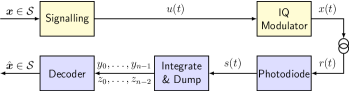
Figure 13: The system model for operation in the O band.

Figure 14: The O-band BER for the constellations highlighted in Table I, at $50~{}$Gbaud, and at a laser power of $2~{}\text{dBm}$. The chromatic dispersion in is $1~{}\text{ps}\cdot\text{nm}^{-1}\cdot\text{km}^{-1}$. Simulations performed with a chromatic dispersion of $-1~{}\text{ps}\cdot\text{nm}^{-1}\cdot\text{km}^{-1}$ gave identical results.

VII Discussion

In contrast to a long-haul or wireless communication system where the power budget of the transmitter and the receiver are decoupled, in short-haul applications the power budget is shared between the transmitter and receiver. As KK schemes use an unsynchronized laser at the receiver—or send a tone along with the signal at transmitter— a fair comparison between KK and direct detection under Tukey signalling or with IMDD should be made under a fixed total power, i.e., including the receiver laser power (or the transmitter tone), as well. As a result, due to the high laser power at the receiver (or high tone power at the transmitter), the KK schemes are not power efficient for communication over short distances, i.e., $<10~{}$km. However, for longer distances, e.g., about $100~{}$km, other imperfections of optical fiber become substantial, necessitating post-detection compensation. In those cases, by recovery of the complex-valued received waveform from its intensity, KK receivers are a matter of interest.

In this paper, we addressed three practical issues which were ignored in [1]. First, we addressed constellation design and decoding complexity by introducing trellis diagrams for SQAM constellations. Second, have included the nonlinearity of the IQ modulator, rather than assuming arbitrary waveform generation. Third, we searched over various $n_{r}$, $n_{p}$, and $\delta$ values to determine which constellations have best performance.

Comparisons with IMDD show that at $50~{}$Gbaud and at a launch power of $-10~{}$dBm, the proposed scheme achieves a throughput of $200~{}$Gb/s using $(8,4)$-SQAM constellation, while at this launch power IMDD achieves $145~{}$Gb/s using PAM-$8$. This increase in the throughput requires implementation of an IQ modulator at the transmitter and two ADCs, each operating at the symbol rate, at the receiver.

References

- [1] A. Tasbihi and F. R. Kschischang, “Direct detection under Tukey signalling,” J. Lightw. Technol., vol. 39, no. 21, pp. 6845–6857, Nov. 2021.
- [2] A. Lender, “The duobinary technique for high-speed data transmission,” IEEE Trans. Commun. Electron., vol. 82, no. 2, pp. 214–218, May 1963.
- [3] P. Kabal and S. Pasupathy, “Partial-response signalling,” IEEE Trans. Commun., vol. 23, no. 9, pp. 921–934, Sep. 1975.
- [4] A. Mecozzi, C. Antonelli, and M. Shtaif, “Kramers-Kronig coherent receiver,” Optica, vol. 3, no. 11, pp. 1220–1227, 2016.
- [5] ——, “Kramers-Kronig receivers,” Adv. Opt. Photon., vol. 11, no. 3, pp. 480–517, 2019.
- [6] T. Bo and H. Kim, “Kramers-Kronig receiver operable without digital upsampling,” Opt. Express, vol. 26, no. 11, pp. 13 810–13 818, 2018.
- [7] K. H. Powers, “The compatibility problem in single-sideband transmission,” Proc. IRE, vol. 48, no. 8, pp. 1431–1435, Aug. 1960.
- [8] B. Logan and M. Schroeder, “A solution to problem of compatible single-sideband transmission,” IRE Trans. Inf. Theory, vol. 8, no. 5, pp. 252–259, Sep. 1962.
- [9] H. B. Voelcker, “Toward a uniform theory of modulation part I: Phase-envelope relationship,” Proc. IEEE, vol. 54, no. 3, pp. 340–353, Mar. 1966.
- [10] ——, “Toward a uniform theory of modulation part II: Zero manipulation,” Proc. IEEE, vol. 54, no. 5, pp. 735–755, May 1966.
- [11] ——, “Demodulation of single-sideband signals via envelope detection,” IEEE Trans. Commun., vol. 14, no. 1, pp. 22–30, Feb. 1966.
- [12] G. B. Lockhart, “A spectral theory for hybrid modulation,” IEEE Trans. Commun., vol. 21, no. 7, pp. 790–800, Jul. 1973.
- [13] G. C. Papen and R. E. Blahut, Lightwave Communications. Cambridge, UK: Cambridge Univ. Press, 2019.
- [14] D. Plabst, T. Prinz, T. Wiegart, T. Rahman, N. Stojanović, S. Calabrò, N. Hanik, and G. Kramer, “Achievable rates for short-reach fiber-optic channels with direct detection,” J. Lightw. Technol., vol. 40, no. 12, pp. 3602–3613, Jun. 2022.
- [15] F. R. Kschischang and V. Sorokine, “On the trellis structure of block codes,” IEEE Trans. Inf. Theory, vol. 41, no. 6, pp. 1924–1937, Nov. 1995.
- [16] G. P. Agrawal, Fiber–Optic Communication Systems, 4th ed. NJ, USA: John Wiley & Sons, 2010.