^†^†thanks: pcappell@mit.edu

A geometric perspective: experimental evaluation of the quantum Cramér-Rao bound

Changhao Li gbsn(李长昊) Research Laboratory of Electronics, Massachusetts Institute of Technology, Cambridge, Massachusetts 02139, USA Department of Nuclear Science and Engineering, Massachusetts Institute of Technology, Cambridge, Massachusetts 02139, USA Mo Chen gbsn(陈墨) Research Laboratory of Electronics, Massachusetts Institute of Technology, Cambridge, Massachusetts 02139, USA Institute for Quantum Information and Matter, California Institute of Technology, Pasadena, CA 91125, USA Thomas J. Watson, Sr., Laboratory of Applied Physics, California Institute of Technology, Pasadena, CA 91125, USA Paola Cappellaro Research Laboratory of Electronics, Massachusetts Institute of Technology, Cambridge, Massachusetts 02139, USA Department of Nuclear Science and Engineering, Massachusetts Institute of Technology, Cambridge, Massachusetts 02139, USA Department of Physics, Massachusetts Institute of Technology, Cambridge, Massachusetts 02139, USA

Abstract

The power of quantum sensing rests on its ultimate precision limit, quantified by the quantum Cramér-Rao bound (QCRB), which can surpass classical bounds. In multi-parameter estimation, the QCRB is not always saturated as the quantum nature of associated observables may lead to their incompatibility. Here we explore the precision limits of multi-parameter estimation through the lens of quantum geometry, enabling us to experimentally evaluate the QCRB via quantum geometry measurements. Focusing on two- and three-parameter estimation, we elucidate how fundamental quantum uncertainty principles prevent the saturation of the bound. By linking a metric of “quantumness” to the system geometric properties, we investigate and experimentally extract the attainable QCRB for three-parameter estimations.

Quantum sensing stands as a key application for quantum technologies Degen et al. (2017). Quantum sensors promise to achieve better sensitivity or precision than classical systems and have been utilized in many fields, ranging from material science Marchiori et al. (2022); Thiel et al. (2019); Yip et al. (2019); Lesik et al. (2019); Hsieh et al. (2019) to biology Kucsko et al. (2013); Choi et al. (2020); Li et al. (2022); Marais et al. (2018). Quantum metrology quantifies the precision limit of quantum sensing with the quantum Cramér-Rao bound (QCRB) Helstrom (1967); Yuen and Lax (1973); Belavkin (1976); Holevo (1977); Carollo et al. (2019); Liu et al. (2019); Albarelli et al. (2020). For unbiased estimation of an unknown system parameter, the QCRB is given by the inverse of the quantum Fisher information Holevo (1977); Carollo et al. (2019); Liu et al. (2019); Albarelli et al. (2020). The estimator is chosen to be optimal, therefore the QCRB only depends on the quantum state. In turn, the precision of estimating a parameter can be linked to the “distance” between two nearby states differing by an infinitesimally small parameter change Braunstein and Caves (1994); Guo et al. (2016); Kolodrubetz et al. (2017); Liu et al. (2019). This naturally connects quantum sensing to the quantum geometric properties of the system, as the quantum metric tensor is closely related to the ultimate estimation precision quantified by the quantum Fisher information.

This picture becomes more involved when extending the goal from estimating a single parameter to multiple parameters, in analogy to the complexity of multi-dimensional system versus 1D systems. The complication arises from the incompatibility between each parameter’s optimal estimators–a signature of quantum mechanics Albarelli et al. (2020); Liu et al. (2019); Guo et al. (2016). This leads to trade-offs among the estimation precisions of different parameters when picking the initial state. This interplay among parameters makes the multi-parameter estimation problem more intriguing than single parameter estimation. Hence developing tools to investigate the ultimate precision and the attainable QCRB in a multi-parameter estimation setting is of great interest for quantum metrology and sensing applications. A promising strategy, similar to the single-parameter scenario, is to link quantum geometric properties of the (multi-)parametrized state to the estimation precision. Specifically, in addition to the link between the quantum metric tensor and the quantum Fisher information, we can link the non-commutativity of optimal measurement operators for different parameters to the Uhlmann curvature Carollo et al. (2019); Liu et al. (2019); Albarelli et al. (2020), as we explain below. Characterizing the geometry of the parametrized quantum states by measuring the quantum geometric tensor would thus help explore the problem of quantum multi-parameter estimation and evaluate the attainable QCRB from a geometric perspective.

In this work, we explore the relation between quantum geometry and multi-parameter estimation to gain novel insight into the corresponding precision bound. In particular, we show that geometric and parameter estimation metrics are connected via the characterization number $\gamma$ , which characterizes the “quantumness” of the system. We find that the characterization number $\gamma$ is linked to both metrology and geometry: $\gamma$ is upper-bounded by the fundamental uncertainty relation and it can be a signature of exotic magnetic monopoles in parameter space. Beyond its theoretical insight, this relation provides a strategy to experimentally evaluate quantum estimation bounds. We can thus provide an experimental demonstration of these results by focusing on a three-parameter, three-level pure state model, which is synthesized using a single nitrogen-vacancy (NV) center in diamond. Based on measuring spin-1 Rabi oscillations upon parameter-modulated driving, we develop experimental tools to extract the geometric quantities and determine the quantum Fisher information and Uhlmann curvature of the quantum state. Then the system’s quantumness, i.e., the incompatibility among parameters to be estimated, is characterized with the help of the characterization number $\gamma$ . We finally evaluate the attainable QCRB for the parameterized state, as well as the two-parameter states in the subspace of the three-parameter model.

Relating quantum geometry to quantum multi-parameter sensing

We consider a generic quantum multi-parameter estimation problem given by a quantum statistic model $\rho_{\boldsymbol{\theta}}$ , a family of density operator labelled by $\boldsymbol{\theta}=(\theta_{1},\theta_{2},...,\theta_{d})^{T}$ that is the set of unknown parameters to be estimated. Performing POVM $\mathcal{M}=\{\mathcal{M}_{k}|\sum_{k}\mathcal{M}_{k}=I,\mathcal{M}_{k}\geq 0\}$ , we obtain the measurement conditional probabilities $p(k|\boldsymbol{\theta})=\textrm{Tr}[\rho_{\boldsymbol{\theta}}\mathcal{M}_{k}]$ . With $N$ repeated measurements, the unknown parameters are estimated via the estimator $\tilde{\boldsymbol{\theta}}(k)$ . The accuracy of the estimation is quantified by the mean-square error matrix $\boldsymbol{V(\boldsymbol{\theta})}=\sum_{k}p(k|\boldsymbol{\theta})[\tilde{\boldsymbol{\theta}}(k)-\boldsymbol{\theta}][\tilde{\boldsymbol{\theta}}(k)-\boldsymbol{\theta}]^{T}$ . Obtaining the lower bounds of this error matrix is of critical importance in quantum sensing and metrology.

The bounds usually depend on the choice of POVM. The symmetric logarithmic derivative Helstrom (1967); Yuen and Lax (1973); Belavkin (1976) (SLD) can be used to define a bound that only depends on the quantum statistic model $\rho_{\boldsymbol{\theta}}$ , having optimized over the measurement operators. The SLD $L_{\mu}$ ( $\mu\in\boldsymbol{\theta}$ ) is implicitly defined via the equation

\partial_{\mu}\rho_{\boldsymbol{\theta}}=\frac{L_{\mu}\rho_{\boldsymbol{\theta}}+\rho_{\boldsymbol{\theta}}L_{\mu}}{2}.

(1)

The corresponding quantum Fisher information matrix (QFIM), $\boldsymbol{J}(\boldsymbol{\theta})$ , is given by

J_{\mu\nu}(\boldsymbol{\theta})=\textrm{Tr}[\rho_{\boldsymbol{\theta}}\frac{L_{\mu}L_{\nu}+L_{\nu}L_{\mu}}{2}],

(2)

which yields the matrix SLD QCRB $\boldsymbol{V(\boldsymbol{\theta})}\geq\boldsymbol{J}(\boldsymbol{\theta})^{-1}$ . It is convenient to introduce a scalar QCRB, $C^{S}(\boldsymbol{\theta},\boldsymbol{W})=\textrm{Tr}\left[{\boldsymbol{W}\boldsymbol{J}(\boldsymbol{\theta})^{-1}}\right]$ . For a weight matrix $\boldsymbol{W}$ , the inequality becomes $\textrm{Tr}\left[{\boldsymbol{W}\boldsymbol{V}}\right]\geq C^{S}(\boldsymbol{\theta},\boldsymbol{W})$ . This SLD-CRB is generally not attainable due to the incompatibility of generators of different parameters. That is, the optimal measurement operators corresponding to different parameters do not commute with each other, making this scalar bound unreachable.

Holevo derived Holevo (1977) a tighter scalar bound, the Holevo Cramér-Rao bound (HCRB) $C^{H}(\boldsymbol{\theta},\boldsymbol{W})$ , which is however only obtained as an optimization. More recently, it has been shown that these two scalar bounds satisfy the following inequality Carollo et al. (2019)

	$\displaystyle C^{S}(\boldsymbol{\theta},\boldsymbol{W})\leq C^{H}(\boldsymbol{\theta},\boldsymbol{W})$	(3)
$\displaystyle\leq$	$\displaystyle C^{S}(\boldsymbol{\theta},\boldsymbol{W})+\|\|\sqrt{\boldsymbol{W}}\boldsymbol{J}^{-1}\boldsymbol{F}\boldsymbol{J}^{-1}\sqrt{\boldsymbol{W}}\|\|_{1}$
$\displaystyle\leq$	$\displaystyle(1+\gamma)C^{S}(\boldsymbol{\theta},\boldsymbol{W})\leq 2C^{S}(\boldsymbol{\theta},\boldsymbol{W}),$

where $||\cdot||_{1}$ denotes the trace norm and $\boldsymbol{F}$ is known as the mean Uhlmann curvature with element $F_{\mu\nu}=-\frac{i}{4}\textrm{Tr}[\rho_{\boldsymbol{\theta}}[L_{\mu},L_{\nu}]]$ (for pure states this reduces to the Berry curvature.) The characterization number $\gamma$ that appears in Eq. (3) is defined as

\gamma=||i2\boldsymbol{J}^{-1}\boldsymbol{F}||_{\infty},

(4)

where $||\boldsymbol{A}||_{\infty}$ denotes the largest eigenvalue of $\boldsymbol{A}$ . $\gamma$ characterizes the “quantumness” of the system, i.e., it quantifies the amount of incompatibility of the statistic model $\rho_{\boldsymbol{\theta}}$ . As implicit in Eq. (3) and explained hereafter, it can be proved that $0\leq\gamma\leq 1$ Carollo et al. (2019).

An explicit expression for an attainable scalar QCRB with weight matrix $\boldsymbol{W}=\boldsymbol{J}$ , which monotonically increases with $\gamma$ , was derived in Ref. Matsumoto (2000, 2002)

	$\displaystyle C(\boldsymbol{\theta})$	$\displaystyle=\textrm{Tr}\left[{\textrm{Re}\left[\sqrt{\openone_{d}+2i\boldsymbol{J}(\boldsymbol{\theta})^{-1/2}\boldsymbol{F}(\boldsymbol{\theta})\boldsymbol{J}(\boldsymbol{\theta})^{-1/2}}\right]^{-2}}\right]$
		$\displaystyle=\sum_{i}\frac{2}{1+\sqrt{1-\|\gamma_{i}\|^{2}}},$		(5)

where $\openone_{d}$ is the d-dimensional identity matrix and $\gamma_{i}$ is the i-th eigenvalue of $i2\boldsymbol{J}^{-1}\boldsymbol{F}$ . The evaluation of this attainable QCRB in terms of geometric quantities, and its relation with SLD-CRB and HCRB, is our key result.

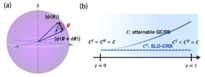
Refer to caption — Figure 1: (a). Diagram showing the “distance” between nearby states $\ket{\psi(\boldsymbol{\theta})}$ and $\ket{\psi(\boldsymbol{\theta}+d\boldsymbol{\theta})}$ in parameter space, from which the metric tensor $\boldsymbol{g}$ (proportional to quantum Fisher information $\boldsymbol{J}$ ) and Berry curvature $\boldsymbol{F}$ naturally arise. (b). SLD-CRB and attaianable QCRB for different $\gamma$ values. At $\gamma=0$ the model is quasi-classical and the SLD-CRB is reachable, i.e., $C^{S}=C^{H}=C$ , while the model is called coherent at $\gamma=1$ with $C^{S}<C^{H}=C$ . Here we take the weight matrix $\boldsymbol{W}=\boldsymbol{J}$ and denote $C^{S(H)}(\boldsymbol{\theta},\boldsymbol{W})$ as $C^{S(H)}$ for simplicity.

To highlight the geometric interpretation of $\boldsymbol{J},\boldsymbol{F}$ (so-far introduced via the SLD) and thus the connection between estimation and geometry, in the following we consider pure state models, i.e., $\rho_{\boldsymbol{\theta}}=\ket{\psi(\boldsymbol{\theta})}\!\bra{\psi(\boldsymbol{\theta})}$ . The geometric properties of this state are captured by the quantum geometric tensor (QGT), which naturally appears when one considers the “distance” between nearby states $\ket{\psi(\boldsymbol{\theta})}$ and $\ket{\psi(\boldsymbol{\theta}+d\boldsymbol{\theta})}$ (Fig. 1):

ds^{2}\equiv 1-|\bra{\psi(\boldsymbol{\theta})}{\psi(\boldsymbol{\theta}\rangle+d\boldsymbol{\theta})}|^{2}=d\theta_{\mu}\chi_{\mu\nu}d\theta_{\nu}+O(|d\boldsymbol{\theta}|^{3}).

Here we defined the QGT, given by $\chi_{\mu\nu}=\bra{\partial_{\mu}\psi}(I-\ket{\psi}\bra{\psi})\ket{\partial_{\nu}\psi}=g_{\mu\nu}+\frac{i}{2}F_{\mu\nu}$ . Its imaginary (antisymmetric) part $F_{\mu\nu}$ is the Berry curvature. The symmetric real part $g_{\mu\nu}$ , also known as Fubini-Study metric tensor, characterizes the overlap between the nearby states. A larger $g_{\mu\nu}$ indicates a larger distinguishability between two states differing by an infinitesimal change of parameters, and it is thus related to a larger quantum Fisher information. The role of the Berry curvature is subtler, as it links the attainability of the QFI bound in multi-parameter scenarios to the observable compatibility.

To show the relation between QGT and parameter estimation, one can assume the parameter $\boldsymbol{\theta}$ to be introduced by evolving an initial state $\ket{\psi_{0}}$ via a unitary evolution, i.e., $\ket{\psi(\boldsymbol{\theta})}=U(\boldsymbol{\theta})\ket{\psi_{0}}$ . Then, the generator for parameter $\mu\in\boldsymbol{\theta}$ is the operator $\mathcal{G}_{\mu}\equiv i(\partial_{\mu}U)U^{\dagger}$ . It can be shown that the QFIM $J_{\mu\nu}$ and the metric tensor $g_{\mu\nu}$ are related by SOM

J_{\mu\mu}\!=\!4\left\langle\Delta\mathcal{G}_{\mu}^{2}\right\rangle\!=\!4g_{\mu\mu},\quad J_{\mu\nu}\!=\!4\mathrm{Cov}(\mathcal{G}_{\mu},\mathcal{G}_{\nu})\!=\!4g_{\mu\nu},

(6)

where $\left\langle\Delta\mathcal{G}_{\mu}^{2}\right\rangle$ is the generator variance and $\mathrm{Cov}(\mathcal{G}_{\mu},\mathcal{G}_{\nu})$ their covariance. Similarly, the Berry curvature is given by the commutator between the parameter generators

F_{\mu\nu}=i\left\langle[\mathcal{G}_{\mu},\mathcal{G}_{\nu}]\right\rangle.

(7)

It is now clear that the Berry curvature matrix characterizes the incompatibility of the system as it arises from the non-commutativity between generators of different parameters. When $F_{\mu\nu}=0$ ( $\forall\mu,\nu\in\boldsymbol{\theta}$ ), the characterization number is $\gamma=0$ according to Eq. 4 and the system is quasi-classical. The discrepancy between the attainable QCRB and the SLD-CRB now vanishes, i.e., $C(\boldsymbol{\theta})=C^{S}(\boldsymbol{\theta},\boldsymbol{J})=C^{H}(\boldsymbol{\theta},\boldsymbol{J})=\textrm{Tr}\left[{\openone_{d}}\right]=d$ .

As one of the main contributions of this letter, we next show that in the opposite limit the characterization number $\gamma$ is upper-bounded by the fundamental quantum uncertainty principles. We consider the two-parameter case and start from the Robertson-Schrödinger uncertainty relation for two operators $\hat{A},\hat{B}$ Robertson (1934), which is the stronger version of the better-known Heisenberg uncertainty relation. In the quantum parameter estimation case, the operators $\hat{A},\hat{B}$ can be replaced by the generators of parameters $\mu,\nu$ , giving

\begin{split}\left\langle\Delta\mathcal{G}_{\mu}^{2}\right\rangle\left\langle\Delta\mathcal{G}_{\nu}^{2}\right\rangle\geq\frac{1}{4}|\left\langle[\mathcal{G}_{\mu},\mathcal{G}_{\nu}]\right\rangle|^{2}+\frac{1}{4}\langle\{\mathcal{G}_{\mu},\mathcal{G}_{\nu}\}\rangle^{2}\\ =\frac{1}{4}|\left\langle[\mathcal{G}_{\mu},\mathcal{G}_{\nu}]\right\rangle|^{2}+\mathrm{Cov}(\mathcal{G}_{\mu},\mathcal{G}_{\nu})^{2}.\end{split}

(8)

With Eq. (4,6,7) we have

\gamma=2\frac{F_{\mu\nu}}{\sqrt{\mathrm{det}(\boldsymbol{J})}}=\frac{1}{2}\frac{F_{\mu\nu}}{\sqrt{\mathrm{det}(\boldsymbol{g})}}\leq 1,

(9)

which relates $\gamma$ to half the Berry’s phase along the curve that encloses a unit area induced by metric tensor. This relation holds for any two-parameter space in a multi-parameter setting. The above relation can also be derived from the fact that the QGT $\chi_{\mu\nu}$ is a positive semi-definite matrix and has been explored in various models Ozawa and Mera (2021); Mera and Ozawa (2021); Mera et al. (2022a). Reversely, generalization of the two-operator product uncertainty relations Eq. 8 to multi-operators can be performed using the fact that $\gamma\leq 1$ , as we show in the supplementary material SOM .

As a concrete example, we consider a two-parameter model in a qubit system $\ket{\psi(\theta,\phi)}=\cos\left(\frac{\theta}{2}\right)\ket{0}-\sin\left(\frac{\theta}{2}\right)e^{-i\phi}\ket{1}$ . The QFIM and Berry curvature matrix,

\boldsymbol{J}=\begin{pmatrix}1&0\\ 0&\sin^{2}\theta\\ \end{pmatrix},\quad\boldsymbol{F}=\begin{pmatrix}0&\sin\theta/2\\ -\sin\theta/2&0\\ \end{pmatrix},

(10)

yield $\gamma=1$ , implying that the model is coherent and the two parameters $\theta,\phi$ here are informationally exclusive. Indeed, they are associated with the non-commuting generators $\sigma_{z}$ and $\sigma_{y}$ , respectively.

Eq. (6-7) show the connection between quantum geometry and quantum multi-parameter estimation (Fig. 1). The value of $\gamma$ characterizes both the quantum multi-parameter estimation scenario, where it is a measure of system’s incompatibility, and the geometry of the quantum state manifold, where it relates the metric tensor determinant to the Berry curvature. This ratio is deeply connected to the existence of topological invariants. Indeed, more generally $\gamma$ can be expressed as the ratio between an $n-$ form generalized Berry curvature $F_{\alpha\beta...}$ and the determinant of the metric tensor, $\gamma=c\frac{F_{\alpha\beta...}}{\sqrt{det(\boldsymbol{g})}}$ with $c$ being a constant normalization factor. Accordingly, $\gamma$ is gauge-invariant and for pointlike or extended monopoles Palumbo and Goldman (2018); Chen et al. (2022), we have $\gamma(\boldsymbol{\theta})=1,$ $\forall\boldsymbol{\theta}$ in parameter space, indicating the largest quantumness of these monopoles. The isotropy of $\gamma$ is due to the radial nature of the field emanating from monopole sources; when $\gamma=1$ , the flux (i.e., the generalized Berry curvature) through an unit area (given by the metric tensor determinant) is unit and thus the flux integral over a closed sphere $S^{n}$ gives the quantized topological number, upon normalization.

As an example, the previous two-parameter, qubit model $\ket{\psi(\theta,\phi)}$ describes pure states on a $S^{2}$ sphere such that the integral of their Berry curvature $F_{\mu\nu}$ over the sphere yields the first Chern number, corresponding to a Dirac monopole at the origin of parameter space.

In the following, we experimentally explore the relation between quantum geometry and quantum multi-parameter estimation. In particular, we measure the geometric quantities using a three-level system and demonstrate the relation (3) and obtain the attainable QCRB. By embedding a two-parameter model into a 3-level system, we can further explore scenarios away from the two bounds $\gamma=0,1$ .

Experiments

We engineer a pure state model using a single nitrogen-vacancy (NV) center in diamond at room temperature. The degeneracy of $\ket{m_{s}=\pm 1}$ is lifted by an external magnetic field $B$ =490 G along the NV quantization axis, which also polarizes the intrinsic nitrogen nuclear spin during optical initialization. This qutrit system can be fully controlled using dual-frequency microwave pulses on-resonance with the transitions between $\ket{m_{s}=0}$ and $\ket{m_{s}=\pm 1}$ . We can thus create any state parametrized by three angles,

\ket{\psi(\alpha,\beta,\phi)}=\frac{1}{\sqrt{2}}\begin{pmatrix}\cos(\alpha)e^{-i\beta}\\ -1\\ \sin(\alpha)e^{-i\phi}\\ \end{pmatrix}.

(11)

We measure the QGT of the this state to determine the QFIM and Berry curvature matrix to characterize both its geometry and multi-parameter estimation properties. Specifically, we measure all the components of the real and imaginary part of the QGT separately using weak modulations of the parameters $\mu,\nu\in\{\alpha,\beta,\phi\}$ , a method that has been explored in previous work Chen et al. (2022); Ozawa and Goldman (2018); Yu et al. (2019). While more details can be found in ref Chen et al. (2022), here we briefly illustrate the principles of the measurement.

To extract the real part of the QGT, we first prepare the state in Eq. (11) with a two-tone microwave pulse after initialization to $\ket{m_{s}=0}$ . We then apply driving with in-phase modulation of the amplitudes $\mu,\nu$ , i.e., $\mu(t)=\mu_{0}+m_{\mu}\sin(\omega t)$ and $\nu(t)=\nu_{0}+m_{\nu}\sin(\omega t)$ with $|m_{\mu}|,|m_{\nu}|\ll 1$ . Similarly, the imaginary part of the QGT can be extracted with out-of-phase modulations, where $\mu(t)=\mu_{0}+m_{\mu}\sin(\omega t)$ and $\nu(t)=\nu_{0}+m_{\nu}\cos(\omega t)$ . These weak periodic modulations of the parameters will drive Rabi oscillations between the state in Eq. (11) and the other two eigenstates of the qutrit system, when the driving frequency $\omega$ is on-resonance with the energy splitting between $\ket{\psi(\alpha,\beta,\phi)}$ and the other two eigenstates $\ket{\psi_{1}}=(-\sin\alpha e^{-i\beta},0,\cos\alpha e^{-i\phi})^{T}$ and $\ket{\psi_{2}}=(\cos\alpha e^{-i\beta},1,\sin\alpha e^{-i\phi})^{T}$ . Following the technique introduced in Ref. Chen et al. (2022), we can extract the QGT, and thus the QFIM, by measuring the resulting Rabi frequencies SOM .

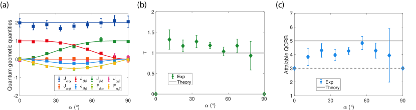
The QGT components reconstructed using this technique are shown in Fig. 2(a). The measurement results are in good agreement with the theoretical predictions derived from the definition of quantum geometry tensor,

\begin{split}\boldsymbol{J}(\alpha,\beta,\phi)=\begin{pmatrix}2&0&0\\ 0&2\cos^{2}(\alpha)-\cos^{4}(\alpha)&-\frac{1}{4}\sin^{2}(2\alpha)\\ 0&-\frac{1}{4}\sin^{2}(2\alpha)&2\sin^{2}(\alpha)-\sin^{4}(\alpha)\\ \end{pmatrix}\end{split}

(12)

and

\begin{split}&\boldsymbol{F}(\alpha,\beta,\phi)=\frac{1}{2}\begin{pmatrix}0&\sin(2\alpha)&-\sin(2\alpha)\\ -\sin(2\alpha)&0&0\\ \sin(2\alpha)&0&0\\ \end{pmatrix}.\\ \end{split}

(13)

The characterization number $\gamma$ can then be determined as in Fig. 2(b). When $\alpha=0$ or $\frac{\pi}{2}$ , the parameterized model Eq. 11 effectively becomes a qubit system in a one-parameter (sub)space. For example, when $\alpha=0$ we have $J_{\phi\phi}=0$ , meaning that we have no information on $\phi$ , and $\boldsymbol{F}=0$ , indicating that there are no non-commuting generators, and the parameter $\beta$ can be estimated trivially. The model is thus quasi-classical. When $\alpha\in(0,\frac{\pi}{2})$ , however, the model is coherent with $\gamma=1$ , indicating the maximal non-commutativity of the generators corresponding to the three parameters.

We can further measure the attainable QCRB, Fig. 2(c). Again, when $\alpha=0$ or $\frac{\pi}{2}$ , the attainable QCRB is equal to the SLD-CRB and HCRB, i.e., $C=C^{S}=C^{H}$ due to the quasi-classical nature of the system. In all other cases, when $\gamma=1$ , the attainable QCRB is equal to the HCRB Matsumoto (2002) and is higher than SLD-CRB due to the incompatibility of the three parameters. From a geometric point of view, this three-level model corresponds to the ground state of a 4D Weyl-type Hamiltonian in spherical coordinates, that hosts a tensor monopole at the origin Chen et al. (2022). We can rewrite the characterization number as

\gamma=2\frac{\sqrt{J_{\phi\phi}F_{\alpha\beta}^{2}+J_{\beta\beta}F_{\alpha\phi}^{2}-2J_{\beta\phi}F_{\alpha\beta}F_{\alpha\phi}}}{\sqrt{\det\boldsymbol{J}}}\equiv\frac{2\mathcal{H}_{\alpha\beta\phi}}{\sqrt{\det\boldsymbol{J}}}.

(14)

When $\gamma=1$ , one recovers the relation between the generalized 3-from curvature $\mathcal{H}$ and metric tensor $\boldsymbol{g}$ , $\mathcal{H}=\frac{1}{2}\sqrt{\det\boldsymbol{J}}=4\sqrt{\det\boldsymbol{g}}$ . The integral of the curvature over the $S^{3}$ sphere yields the Dixmier-Douady invariant, which is the topological number for a tensor monopole and its related Kalb-Ramond field Chen et al. (2022); Palumbo and Goldman (2018).

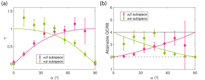
The above three-parameter model enables us to study both quasi-classical ( $\gamma=0$ ) and coherent ( $\gamma=1$ ) cases. That model, as well as the two-level model $\ket{\psi(\theta,\phi)}=\cos\left(\frac{\theta}{2}\right)\ket{0}-\sin\left(\frac{\theta}{2}\right)e^{-i\phi}\ket{1}$ , is indeed one of the eigenstates of a gapless Weyl-type Hamiltonian that hosts monopoles at the origin of parameter space Mera et al. (2022a); Chen et al. (2022), leading to $\gamma=1$ (or 0 at special points). To study intermediate cases where $\gamma\leq 1$ , one can consider different geometrical models Mera et al. (2022b) or, as done here, rely on the two-parameter subspaces of the above three-parameter model where $\gamma$ is a function of $\alpha$ . From the viewpoint of the Hamiltonian, this corresponds to taking a slice of the original gapless Weyl-type system, which yields a gapped topological insulator that can have $\gamma\leq 1$ . We thus now revisit the problem of two-parameter estimation in the subspace of the qutrit system. Specifically, we focus on the subspace spanned by parameters $(\alpha,\beta)$ and $(\alpha,\phi)$ (the $(\beta,\phi)$ subspace is trivial since all the corresponding Berry curvature components are zero and the SLD-CRB is attainable.) In Fig. 3 we plot the characterization number $\gamma$ as well as the corresponding attainable QCRB. When $\alpha=0(\frac{\pi}{2})$ , the three-level system effectively reduces to a two-level system and the parameter $\phi$ ( $\beta$ ) cannot be estimated due to the null population in $[0,0,1]^{T}$ ( $[1,0,0]^{T}$ ). We observe $\gamma$ vary continuously from 0 to 1 when sweeping $\alpha$ in the two subspaces. The HCRB thus ranges from 2, equal to the scalar SLD-CRB, (asymptotically) to 4, where the attainable scalar QCRB is largest (two times larger than the SLD-CRB, as bounded by Eq. 3). These results show how $\gamma$ directly predicts the attainable QCRB for subspace models, and thus sets the estimation precision when evaluating a subset of parameters. The analysis above can then be applied to scenarios where there are nuisance parameters, i.e., parameters that are not of interest but nevertheless affect the precision of estimating other parameters of interest Yang et al. (2019); Suzuki (2020); Suzuki et al. (2020).

While we consider a three-parameter model here, the techniques can be extended to higher dimensional models (beyond three parameters.) For example, we find that $\gamma=1$ for the pure-state, four-parameter space model

\ket{\psi(\alpha,\phi_{1},\phi_{2},\phi_{3})}=\frac{1}{\sqrt{3}}\begin{pmatrix}\cos\alpha e^{i\phi_{1}}\\ e^{i\phi_{2}}\\ \sin\alpha e^{i\phi_{3}}\\ 1\\ \end{pmatrix},

(15)

and similarly, in the subspace spanned by $(\alpha,\phi_{1},\phi_{2})$ and $(\alpha,\phi_{2},\phi_{3})$ , $\gamma$ varies from 0 to 1. Similar to Eq. (14), we find the relation $\gamma=2\frac{\mathcal{E}_{\alpha\phi_{1}\phi_{2}\phi_{3}}}{\sqrt{det{\boldsymbol{J}}}}=1$ where $\mathcal{E}_{\alpha\phi_{1}\phi_{2}\phi_{3}}$ is the 4-form generalized Berry curvature SOM . Its integral over the $S^{4}$ sphere will yield a topological number which is directly proportional to the second Chern number of a 5D tensor monopole Yang (1978); Hasebe (2014); Palumbo and Goldman (2019).

In conclusion, we explore the relation between quantum geometry and quantum multi-parameter estimation. In addition to further insight into the ultimate precision limits, this relation enables us to experimentally extract the attainable scalar quantum Cramér-Rao bound for a three-parameter pure state model synthesized in a single spin system. We show that the SLD-CRB is not reachable due to the non-commutativity of parameter generators that affect the uncertainty relations of quantum mechanics. This bound is clarified through the link to quantum geometry, where the system properties is characterized not only the distance between states (the Fubini-Study metric tensor), but also by the space curvature. The present technique and discussions can provide tools and insights for finding optimal measurement strategies and evaluating the ultimate precision of multi-parameter models Albarelli et al. (2020); Yu et al. (2020); Hou et al. (2020, 2021).

Acknowledgements

This work is supported in part by ARO grant W911NF-11-1-0400 and NSF grant PHY1734011.

References

Degen et al. (2017) C. L. Degen, F. Reinhard, and P. Cappellaro, Rev. Mod. Phys. 89, 035002 (2017).
Marchiori et al. (2022) E. Marchiori, L. Ceccarelli, N. Rossi, L. Lorenzelli, C. L. Degen, and M. Poggio, Nature Reviews Physics 4, 49 (2022).
Thiel et al. (2019) L. Thiel, Z. Wang, M. A. Tschudin, D. Rohner, I. Gutiérrez-Lezama, N. Ubrig, M. Gibertini, E. Giannini, A. F. Morpurgo, and P. Maletinsky, Science 364, 973 (2019).
Yip et al. (2019) K. Y. Yip, K. O. Ho, K. Y. Yu, Y. Chen, W. Zhang, S. Kasahara, Y. Mizukami, T. Shibauchi, Y. Matsuda, S. K. Goh, and S. Yang, Science 366, 1355 (2019).
Lesik et al. (2019) M. Lesik, T. Plisson, L. Toraille, J. Renaud, F. Occelli, M. Schmidt, O. Salord, A. Delobbe, T. Debuisschert, L. Rondin, P. Loubeyre, and J.-F. Roch, Science 366, 1359 (2019).
Hsieh et al. (2019) S. Hsieh, P. Bhattacharyya, C. Zu, T. Mittiga, T. J. Smart, F. Machado, B. Kobrin, T. O. Höhn, N. Z. Rui, M. Kamrani, S. Chatterjee, S. Choi, M. Zaletel, V. V. Struzhkin, J. E. Moore, V. I. Levitas, R. Jeanloz, and N. Y. Yao, Science 366, 1349 (2019).
Kucsko et al. (2013) G. Kucsko, P. C. Maurer, N. Y. Yao, M. Kubo, H. J. Noh, P. K. Lo, H. Park, and M. D. Lukin, Nature 500, 54 (2013).
Choi et al. (2020) J. Choi, H. Zhou, R. Landig, H.-Y. Wu, X. Yu, S. E. V. Stetina, G. Kucsko, S. E. Mango, D. J. Needleman, A. D. T. Samuel, P. C. Maurer, H. Park, and M. D. Lukin, Proceedings of the National Academy of Sciences 117, 14636 (2020).
Li et al. (2022) C. Li, R. Soleyman, M. Kohandel, and P. Cappellaro, Nano Letters, Nano Letters 22, 43 (2022).
Marais et al. (2018) A. Marais, B. Adams, A. K. Ringsmuth, M. Ferretti, J. M. Gruber, R. Hendrikx, M. Schuld, S. L. Smith, I. Sinayskiy, T. P. J. Krüger, F. Petruccione, and R. van Grondelle, Journal of The Royal Society Interface 15, 20180640 (2018).
Helstrom (1967) C. Helstrom, Physics Letters A 25, 101 (1967).
Yuen and Lax (1973) H. Yuen and M. Lax, IEEE Transactions on Information Theory 19, 740 (1973).
Belavkin (1976) V. P. Belavkin, Theoretical and Mathematical Physics 26, 213 (1976).
Holevo (1977) A. Holevo, Reports on Mathematical Physics 12, 251 (1977).
Carollo et al. (2019) A. Carollo, B. Spagnolo, A. A. Dubkov, and D. Valenti, Journal of Statistical Mechanics: Theory and Experiment 2019, 094010 (2019).
Liu et al. (2019) J. Liu, H. Yuan, X.-M. Lu, and X. Wang, Journal of Physics A: Mathematical and Theoretical 53, 023001 (2019).
Albarelli et al. (2020) F. Albarelli, M. Barbieri, M. Genoni, and I. Gianani, Physics Letters A 384, 126311 (2020).
Braunstein and Caves (1994) S. L. Braunstein and C. M. Caves, Phys. Rev. Lett. 72, 3439 (1994).
Guo et al. (2016) W. Guo, W. Zhong, X.-X. Jing, L.-B. Fu, and X. Wang, Phys. Rev. A 93, 042115 (2016).
Kolodrubetz et al. (2017) M. Kolodrubetz, D. Sels, P. Mehta, and A. Polkovnikov, Physics Reports 697, 1 (2017), geometry and non-adiabatic response in quantum and classical systems.
Matsumoto (2000) K. Matsumoto, “Berry’s phase in view of quantum estimation theory, and its intrinsic relation with the complex structure,” (2000), arXiv:quant-ph/0006076 .
Matsumoto (2002) K. Matsumoto, Journal of Physics A: Mathematical and General 35, 3111 (2002).
(23) See supplementary online material.
Robertson (1934) H. P. Robertson, Phys. Rev. 46, 794 (1934).
Ozawa and Mera (2021) T. Ozawa and B. Mera, Phys. Rev. B 104, 045103 (2021).
Mera and Ozawa (2021) B. Mera and T. Ozawa, Phys. Rev. B 104, 045104 (2021).
Mera et al. (2022a) B. Mera, A. Zhang, and N. Goldman, SciPost Phys. 12, 18 (2022a).
Palumbo and Goldman (2018) G. Palumbo and N. Goldman, Phys. Rev. Lett. 121, 170401 (2018).
Chen et al. (2022) M. Chen, C. Li, G. Palumbo, Y.-Q. Zhu, N. Goldman, and P. Cappellaro, Science 375, 1017 (2022).
Ozawa and Goldman (2018) T. Ozawa and N. Goldman, Phys. Rev. B 97, 201117 (2018).
Yu et al. (2019) M. Yu, P. Yang, M. Gong, Q. Cao, Q. Lu, H. Liu, S. Zhang, M. B. Plenio, F. Jelezko, T. Ozawa, N. Goldman, and J. Cai, National Science Review 7, 254 (2019).
Mera et al. (2022b) B. Mera, A. Zhang, and N. Goldman, SciPost Phys. 12, 18 (2022b).
Yang et al. (2019) Y. Yang, G. Chiribella, and M. Hayashi, Communications in Mathematical Physics 368, 223 (2019).
Suzuki (2020) J. Suzuki, Journal of Physics A: Mathematical and Theoretical 53, 264001 (2020).
Suzuki et al. (2020) J. Suzuki, Y. Yang, and M. Hayashi, Journal of Physics A: Mathematical and Theoretical 53, 453001 (2020).
Yang (1978) C. N. Yang, Journal of Mathematical Physics, Journal of Mathematical Physics 19, 320 (1978).
Hasebe (2014) K. Hasebe, Nuclear Physics B 886, 952 (2014).
Palumbo and Goldman (2019) G. Palumbo and N. Goldman, Phys. Rev. B 99, 045154 (2019).
Yu et al. (2020) M. Yu, Y. Liu, P. Yang, M. Gong, Q. Cao, S. Zhang, H. Liu, M. Heyl, T. Ozawa, N. Goldman, and J. Cai, “Quantum fisher information measurement and verification of the quantum cramer-rao bound in a solid-state qubit,” (2020).
Hou et al. (2020) Z. Hou, Z. Zhang, G.-Y. Xiang, C.-F. Li, G.-C. Guo, H. Chen, L. Liu, and H. Yuan, Phys. Rev. Lett. 125, 020501 (2020).
Hou et al. (2021) Z. Hou, J.-F. Tang, H. Chen, H. Yuan, G.-Y. Xiang, C.-F. Li, and G.-C. Guo, Science Advances 7 (2021), 10.1126/sciadv.abd2986.

See pages 1 of SOM.pdf See pages 2 of SOM.pdf See pages 3 of SOM.pdf See pages 4 of SOM.pdf See pages 5 of SOM.pdf See pages 6 of SOM.pdf See pages 7 of SOM.pdf