Triformer: Triangular, Variable-Specific Attentions for Long Sequence Multivariate Time Series Forecasting–Full Version

Abstract

A variety of real-world applications rely on far future information to make decisions, thus calling for efficient and accurate long sequence multivariate time series forecasting. While recent attention-based forecasting models show strong abilities in capturing long-term dependencies, they still suffer from two key limitations. First, canonical self attention has a quadratic complexity w.r.t. the input time series length, thus falling short in efficiency. Second, different variables’ time series often have distinct temporal dynamics, which existing studies fail to capture, as they use the same model parameter space, e.g., projection matrices, for all variables’ time series, thus falling short in accuracy.

To ensure high efficiency and accuracy, we propose Triformer, a triangular, variable-specific attention. (i) Linear complexity: we introduce a novel patch attention with linear complexity. When stacking multiple layers of the patch attentions, a triangular structure is proposed such that the layer sizes shrink exponentially, thus maintaining linear complexity. (ii) Variable-specific parameters: we propose a light-weight method to enable distinct sets of model parameters for different variables’ time series to enhance accuracy without compromising efficiency and memory usage. Strong empirical evidence on four datasets from multiple domains justifies our design choices, and it demonstrates that Triformer outperforms state-of-the-art methods w.r.t. both accuracy and efficiency.

1 Introduction

Long sequence multivariate time series forecasting plays an essential role in planning and managing complex systems across diverse domains Liu et al. (2018); Guo et al. (2020); Pedersen et al. (2020b, a). In such settings, multiple sensors are often deployed to collect diverse information related to a complex system, thus giving rise to multivariate time series Cirstea et al. (2019). Figure 1 shows an example of a 3-variate time series indicating the power consumption of three clients from a power grid system, where each variable has its own time series.

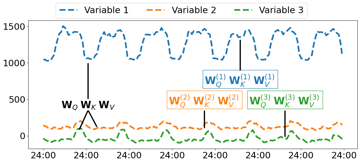
Figure 1: Example of 3-variate time series, where each variable has a distinct temporal pattern. Variable-agnostic modeling: same projection matrices (see the black matrices) are employed for all variables. Variable-specific modeling: distinct projection matrices (see the colorful matrices) are used for different variables, thus enabling the capture of distinct temporal patterns of different variables.

While extensive studies on short term forecasting exist, e.g., dozens steps ahead forecasting Hochreiter and Schmidhuber (1997); Qin et al. (2017); Wu et al. (2019, 2020), a limited number of studies focus on long term forecasting, e.g., hundreds steps ahead. Recent studies show that attentions Vaswani et al. (2017); Wu et al. (2022) are able to capture better long term dependencies, comparing to Recurrent Neural Networks RNNs Li et al. (2018); Hu et al. (2020); Kieu et al. (2022a) or Temporal Convolutional Networks TCNs Wu et al. (2019); Campos et al. (2022); Kieu et al. (2022b). However, two main limitations still exist.

High complexity: For a time series of $H$ timestamps, canonical self-attention has a quadratic complexity of $\mathcal{O}(H^{2})$. Recent studies on long-term forecasting propose different “sparse” versions of self-attentions Zhou et al. (2021); Kitaev et al. (2020), aiming at reducing the high complexity. We propose Triformer with linear complexity $\mathcal{O}(H)$. We first break the time series into small patches. For each patch, we define a novel Patch Attention (PA) with linear complexity (cf. the small white triangles in Figure 2). Specifically, we introduce a pseudo timestamp for a patch and we compute attentions of the timestamps in the patch only to the single pseudo timestamp, making patch attention linear. Then, only the pseudo timestamps are fed into the next layer, such that the layer sizes shrink exponentially, making a triangular structure as shown in Figure 2. This ensures a multi-layer Triformer still have linear complexity $\mathcal{O}(H)$.

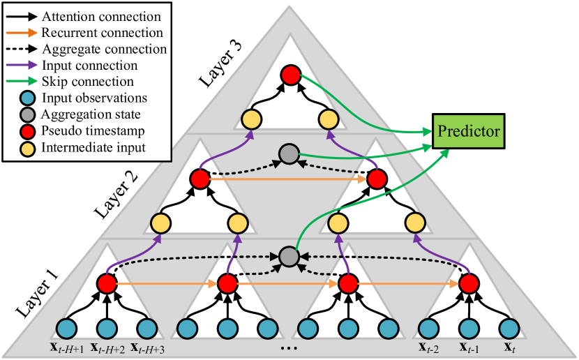
Figure 2: Triformer has a triangular structure as the layer input sizes shrink exponentially, making a multi-layer Triformer still with $\mathcal{O}(H)$.

Variable-agnostic parameters: Existing forecasting models often use variable-agnostic parameters, although different variables may exhibit distinct temporal patterns Wu et al. (2019); Li et al. (2018); Wu et al. (2022). For example, as shown in Figure 1, although variable 1 has a unique temporal pattern, which is different from the patterns of variables 2 and 3, the same model parameters, e.g., the projection matrices $\textbf{W}_{Q},\textbf{W}_{K}$, and $\textbf{W}_{V}$ used in self-attentions (cf. the black matrices in Figure 1), are applied to all three variables. This forces the learned parameters to capture an “average” pattern among all the variables, thus failing to capture distinct temporal pattern of each variable and hurting accuracy.

We propose a light-weight method to enable variable specific parameters, e.g., a distinct set of matrices $\textbf{W}_{Q}^{(i)},\textbf{W}_{K}^{(i)}$, and $\textbf{W}_{V}^{(i)}$ for the $i$-th variable (cf. the colorful matrices in Figure 1), such that it is possible to capture distinct temporal patterns for different variables. Specifically, we factorize the projection matrices into variable-agnostic and variable-specific matrices, where the former are shared among all variables and the latter are specific to different variables. We judiciously make the variable-specific matrices very compact, thus avoiding increasing the parameter space and computation overhead.

We summarize the main contributions as follows: (i) We propose a novel, efficient attention mechanism, namely Patch Attention, along with its triangular, multi-layer structure. This ensures an overall linear complexity, thus achieving high efficiency. (ii) We propose a light-weight approach to enable variable-specific model parameters, making it possible to capture distinct temporal patterns from different variables, thus enhancing accuracy. (iii) We conduct extensive experiments on four public, commonly used multivariate time series data sets from different domains, justifying our design choices and demonstrating that the proposal outperforms state-of-the-art methods.

2 Related Work

We categorize multivariate time series forecasting methods in Table 1 along two dimensions—short vs. long term forecasting and variable-agnostic vs. variable-specific modeling.

	Short Term	Long Term
Variable  Agnostic	Wu et al. (2021) Cao et al. (2020) Bai et al. (2019) Wu et al. (2019) Li et al. (2018)	Zhou et al. (2021) Kitaev et al. (2020) Li et al. (2019) Stoller et al. (2020) Vaswani et al. (2017)
Variable  Specific	Cirstea et al. (2022) Cirstea et al. (2021) Bai et al. (2020) Pan et al. (2019)	Triformer

Table 1: Categorization of Time Series Forecasting.

Short vs. Long Term Forecasting: Most studies focus on short-term forecasting, e.g., 12 to 48 steps ahead. Short-term forecasting models often rely on two types of models that are good at capturing short-term temporal dependencies—recurrent neural networks (RNNs), e.g., LSTM or GRU Bai et al. (2019); Li et al. (2018); Seo et al. (2018), and temporal convolutions networks (TCNs), e.g., 1D convolution and WaveNet Cao et al. (2020); Wu et al. (2019). Both RNNs and TCNs have limited capabilities when dealing with long-range dependencies since they can not directly access the whole input time series, as they rely on intermediate representations Khandelwal et al. (2018). Thus, they fall short on long-term forecasting.

For long term forecasting, self-attention based models achieve superior accuracy, but they suffer from quadratic memory and runtime overhead w.r.t. the input time series length $H$. To reduce the complexity, recent long term forecasting studies propose sparse attentions: LogTrans Li et al. (2019) is with $\mathcal{O}(H(\log H)^{2})$, and Informer Zhou et al. (2021) further reduces the complexity to $\mathcal{O}(H\log H)$. There also exist other efficient versions of attentions Beltagy et al. (2020); Wang et al. (2020); Katharopoulos et al. (2020), but they are not designed and verified for time series forecasting. When stacking multiple layers of attentions, an additional pooling layer is often used after each attention layer. This helps shrink the input size to the next attention layer, thus reducing overall complexity Dai et al. (2020); Zhou et al. (2021). We propose a novel efficient patch attention with linear complexity, which is able to shrink the layer size by itself without using additional pooling, making a multi-layer patch attention structure also linear.

Variable-agnostic vs. variable-specific modeling: Most of the related studies are variable agnostic, meaning that, although different variables’ time series may exhibit distinct temporal patterns, they share the same sets of model parameters, e.g., the same weight matrices in RNNs, the same convolution kernels in TCNs, or the same projection matrices in attentions. Four studies Cirstea et al. (2021, 2022); Bai et al. (2020); Pan et al. (2019) propose variable-specific modeling for RNNs. Specifically, Cirstea et al. Cirstea et al. (2022, 2021) proposed generating variable-specific weight matrices using learned embedding and hyper-networks, however such methods are memory intensive and not suitable for long term forecasting. Pan et al. Pan et al. (2019) generates variable-specific weight matrices using additional meta-information, e.g., categories of points of interest around the deployed sensor locations. However, such additional meta-information may not be always available. Bai et al. Bai et al. (2020) learns variable-specific weight matrices using a purely data-driven manner without additional information. We empirically compare with Bai et al. Bai et al. (2020) in the experiments.

Key differences from pooling based transformers: Pooling based transformers such as Dai et al. (2020); Zhou et al. (2021) utilize self-attention as their core component for harvesting temporal dependencies within the data. Self-attention implicitly assumes that each timestamp needs to act as Query, while harvesting information from all the other timestamps which act as Key (thus the name self-attention). Such design implicitly assumes that each Query needs to be dynamic thus conditioned on the input. While such property might be desirable, it has high complexity as each Query needs to attend each Key having quadratic complexity in the case of Dai et al. (2020) or $\mathcal{O}(S\;log(S))$ for Zhou et al. (2021) (see Figure 4(a)). In contrast our proposed Patch-Attention (PA) is design on the assumption that a static Query has enough representation power such that, once learned, it can solemnly attend to all Keys (see Figure 4(b)). By doing so, not only we reduce the time complexity to linear but we make an attempt into a new direction which does not rely on self-attentions.

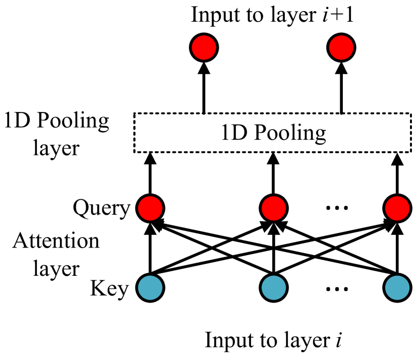
(a) Self-attention, $\mathcal{O}(S^{2})$

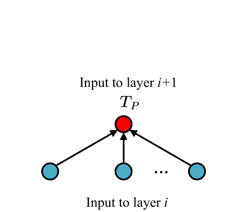
(b) Patch attention, $\mathcal{O}(S)$

Figure 3: Pooling based transformer with self-attention (SA) vs. patch attention (PA) on patch $p$. In SA, each timestamp attends to all other timestamps, thus having $\mathcal{O}(S^{2})$. In PA, each timestamp only attends to the pseudo timestamp, thus having $\mathcal{O}(S)$. In addition, in SA, a pooling layer is applied after each self-attention layer to reduce the input size for the next layer. PA does not need pooling anymore, and a learnable Query per patch is fed into the next layer.

Another important difference is on multi-layer structures. To improve model capacity, multiple layers of attentions are stacked together. To improve efficiency, it is beneficial to shrink the input sizes of the layers. Our proposal differs from pooling based transformers on the layer size shrinking mechanism. In pooling based transformers, a pooling layer is applied after each self-attention layer, as shown in Figure 4(a). The 1D pooling on the temporal axis reduces the size to the next layer. In contrast, our proposed method does not use any pooling mechanism—for each path, we only allow the learnable Query to move to the next layer after it is updated with information from all Keys. Thus, the size to the next layer is reduced by $1/S$.

Key differences from hierarchical transformers: We design PA inspired by hierarchical transformers such as Pappagari et al. (2019); Dosovitskiy et al. (2021); Pan et al. (2021). While the concept might be similar, there are notable differences between the approaches. First, the previously mentioned studies are design for Nature Language Processing and Computer Vision domains, while our method focuses on time-series. Second the previous mentioned studies try to capture dependencies between different patches, thus resulting in a quadratic complexity w.r.t. the number of patches. In contrast, we propose to introduce a learnable pseudo-timestamp for each patch, such that all timestamps within a specific patch can write useful information inside. By doing to we reduce the complexity to linear even after stacking multiple layers.

3 Preliminaries

Problem Definition. A multivariate time series records the values of $N$ variables over time. Observation $\textbf{x}_{t}\in\mathbb{R}^{N}$ denotes the values of all $N$ variables at timestamp $t$ and $\textbf{x}^{(i)}_{t}\in\mathbb{R}$ is the value of the $i$-th variable at $t$. Time series forecasting learns a function $\mathcal{F}$ that takes as into the observations in the historical $H$ timestamps and predicts the future $F$ timestamps.

$$\mathcal{F}_{\phi}(\mathbf{x}_{t-H+1},...,\mathbf{x}_{t-1},\mathbf{x}_{t})=(\mathbf{\hat{x}}_{t+1},\mathbf{\hat{x}}_{t+2},...,\mathbf{\hat{x}}_{t+F}),$$ (1)

where $\phi$ denotes the learnable parameters of the forecasting model and $\mathbf{\hat{x}}_{j}$ is the predicted values at timestamp $j$.

Self-attention. Self-attention is a core operation in attention based models. Given a sequence, e.g., a time series, each timestamp attends to all timestamps in the time series, thus being able to derive a representation of the entire time series by capturing both long- and short-term dependencies. Consider a time series with $H$ timestamps, e.g., time series $\mathbf{x}^{(i)}\in\mathbb{R}^{H}$ from the $i$-th variable. Canonical self-attention Vaswani et al. (2017) first transforms the time series into a query matrix $\mathbf{Q}^{(i)}=\mathbf{x}^{(i)}\mathbf{W}_{Q}\in\mathbb{R}^{H\times d}$, a key matrix $\mathbf{K}^{(i)}=\mathbf{x}^{(i)}\mathbf{W}_{K}\in\mathbb{R}^{H\times d}$ and a value matrix $\mathbf{V}^{(i)}=\mathbf{x}^{(i)}\mathbf{W}_{V}\in\mathbb{R}^{H\times d}$, where $d$ represents the hidden representation and $\mathbf{W}_{Q},\mathbf{W}_{K}$, $\mathbf{W}_{V}\in\mathbb{R}^{d\times d}$ are projection matrices, which are learnable. Next, the output is represented as a weighted sum of the values in the value matrix $\mathbf{V}^{(i)}$, where the weights, a.k.a., attention scores, are computed based on the query matrix $\mathbf{Q}^{(i)}$ and the key matrix $\mathbf{K}^{(i)}$, as shown in Equation 2.

$$\mathcal{A}(\mathbf{Q}^{(i)},\mathbf{K}^{(i)},\mathbf{V}^{(i)})=\varphi(\frac{\mathbf{Q}^{(i)}\textbf{K}^{(i)T}}{\sqrt{d}})\mathbf{V}^{(i)},$$ (2)

where $\varphi$ represents the softmax activation function. Computing the attention scores requires quadratic $\mathcal{O}(H^{2})$ time complexity and memory usage, which is a major drawback. Sparse versions of self-attentions exist, Li et al. (2019); Kitaev et al. (2020); Zhou et al. (2021), reducing the complexity to $\mathcal{O}(Hlog(H)^{2})$ and $\mathcal{O}(H{\cdot}\log H)$. We strive for linear complexity. In addition, in related attention based works, the same projection matrices $\mathbf{W}_{Q}$, $\mathbf{W}_{K}$ and $\mathbf{W}_{V}$ are applied to all variables $\mathbf{x}^{(i)}$ for $1\leq i\leq N$. In contrast, we strive for variable-specific projection matrices.

4 Triformer

We propose Triformer for learning long-term and multi-scale dependencies in multivariate time series. An overview of the Triformer is shown in Figure 2. The design choices of Triformer are three-fold. First, we propose an efficient Patch Attention with linear complexity as the basic building block. Second, we propose a triangular structure when stacking multiple layers of patch attentions, such that the layer sizes shrink exponentially. This ensures linear complexity for multi-layer patch attentions and also enables extracting multi-scale features. Third, we propose a light-weight method to enable variable specific modeling, thus being able to capture distinct temporal patterns from different variables, without compromising efficiency. We proceed to cover the specifics of the three design choices.

4.1 Linear Patch Attention

To contend with the high complexity, we propose an efficient Patch Attention with linear complexity, to ensure competitive overall efficiency. Inspired by Pan et al. (2021), we break down the input time series of length $H$ into $P=H/S$ patches along the temporal dimension, where $S$ is the patch size. Figure 2 shows an example input time series of length $H=12$ being split into $P=4$ patches with patch size $S=3$. We use $\textbf{x}_{p}=\langle\textbf{x}_{(p-1)\cdot S+1},\ldots,\textbf{x}_{p\cdot S}\rangle$ to denote the $p$-th patch.

Based on the patches, we compute attention scores per patch. If we naively use self-attention in a patch, we still have quadratic complexity (cf. Figure 4(a)).

To reduce the complexity to linear, for each patch $p$, we introduce a learnable, pseudo timestamp $\textbf{T}_{p}\in\mathbb{R}^{N\times d}$ (cf. Figure 4(b)). The pseudo timestamp acts as a data placeholder where all the timestamps from the patch can write useful information which is then passed to the next layers. In Triformer, we choose to use the attention mechanism to update the pseudo timestamp, where the pseudo timestamp works as the Query in self-attentions. The pseudo timestamp queries all the “real” timestamps in the patch, thus only computing a single attention score for each real timestamp, giving rise to linear complexity. We call this Patch Attention (PA).

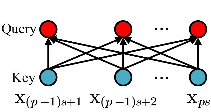
(a) Self-attention, $\mathcal{O}(S^{2})$

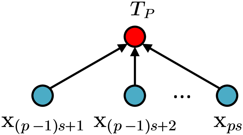
(b) Patch attention, $\mathcal{O}(S)$

Figure 4: Computing self-attention (SA) vs. patch attention (PA) on patch $p$. In SA, each timestamp attends to all other timestamps, thus having $\mathcal{O}(S^{2})$. In PA, each timestamp only attends to the pseudo timestamp, thus having $\mathcal{O}(S)$.

Equation 3 elaborates the computations of PA for pseudo timestamp $\textbf{T}_{p}$. Note that $\textbf{T}_{p}=\{\textbf{T}_{p}^{(i)}\}_{i=1}^{N}$ and each variable has specific pseudo timestamp $\textbf{T}_{p}^{(i)}$, thus being variable-specific.

$$\small\textbf{T}_{p}=\mathcal{PA}(\mathbf{T}_{p},\mathbf{x}_{p})=\Bigg{\{}\varphi(\frac{\mathbf{T}^{(i)}_{p}(\textbf{x}_{p}^{(i)}\textbf{W}_{K})^{T}}{\sqrt{d}})(\textbf{x}_{p}^{(i)}\textbf{W}_{V})\Bigg{\}}_{i=1}^{N}$$ (3)

The reduced complexity of PA comes with a price that the temporal receptive filed of each timestamp is reduced to the patch size $S$. In contrast, in the canonical attention, it is $H$ covering all timestamps. This makes it harder to capture relationships among different patches and also the long-term dependencies, thus adversely affecting accuracy. To compensate for the reduced temporal receptive field, we introduce a recurrent connection (cf. the orange arrows in Figure 2) to connect the outputs of the patches, i.e., the updated pseudo timestamps according to Equation 3, such that the temporal information flow is maintained.

As gating mechanism is a crucial component for recurrent networks and has been showed to be powerful controlling the information flow Dauphin et al. (2017), we propose a gating rule in the recurrent connections in Equation 4.

$$\textbf{T}_{p+1}=g(\boldsymbol{\Theta}_{1}\textbf{T}_{p}+\textbf{b}_{1})\odot\sigma(\boldsymbol{\Theta}_{2}\textbf{T}_{p}+\textbf{b}_{2})+\textbf{T}_{p+1},$$ (4)

where $\boldsymbol{\Theta}_{1}$, $\boldsymbol{\Theta}_{2}$, $\textbf{b}_{1}$ and $\textbf{b}_{2}$ are learned parameters for the recurrent gates, $\odot$ is element-wise product, $g(\cdot)$ is tanh activation function and $\sigma(\cdot)$ is a sigmoid function controlling the information ratio that is passed to the next pseudo timestamp.

4.2 Triangular Stacking

Stacking multiple layers of attention often help improve accuracy. In attention based models, each attention layer has the same input size, e.g., the input time series size $H$. In traditional self-attention same input and output have the same shape. Differently pooling-based methods are applying 1D convolution to the output to shrink the temporal horizon. When using PAs, we only feed the pseudo timestamps from the patches to the next layer, which shrinks the layer sizes exponentially. More specifically, the size of $(l+1)$-th layer is only $\frac{1}{S_{l}}$ of the size of the $l$-th layer, where $S_{l}$ is the patch size of the $l$-th layer. This leads to Lemma 1.

Lemma 1. An $L$-layer Triformer has a linear time complexity $\mathcal{O}(H)$ if patch size $S_{l}\geq 2$ where $1\leq l\leq L$.

Proof. The input size of the $l$-th layer is at most $\frac{H}{\hat{S}^{l-1}}$, where $\hat{S}=\min_{1\leq i\leq L}S_{i}$ is the minimum patch size of all layers. Then, for an $L$-layer TRACE, the sum of the input sizes of all layers is at most $2{\cdot}H$ because

$$\sum_{i=1}^{L}\frac{H}{\hat{S}^{i-1}}=H\cdot\sum_{i=1}^{L}(\frac{1}{\hat{S}})^{i-1}<\frac{\hat{S}}{\hat{S}-1}\cdot H<2\cdot H,$$

where the first inequality holds because $(\frac{1}{\hat{S}})^{i-1}$ forms an exponential series and $\frac{1}{\hat{S}}<1$ and the second inequality hold due to $\hat{S}$ is at least 2. Since the PA has a linear complexity w.r.t. the input size. Thus, the complexity of $L$ layers of PAs is still linear $\mathcal{O}(H)$.

In a multi-layer Triformer, each layer consists of different numbers of patches and thus having different number of outputs, i.e., pseudo timestamps. Instead of only using the last pseudo timestamp per layer, we aggregate all pseudo timestamps per layer into an aggregated output. More specifically, the aggregate output $\textbf{O}^{l}$ at the $l$-th layer is defined as

$$\textbf{O}^{l}=\theta^{l}(\textbf{T}_{1}^{l},..,\textbf{T}_{k}^{l},...,\textbf{T}_{P}^{l}),$$ (5)

where $\theta^{l}$ is a neural network, $\textbf{T}_{p}^{l}$ denotes the pseudo timestamp for patch $p\in[1,P]$ at the $l$-th layer.

Finally, the aggregate outputs from all layers are connected to the predictor. This brings two benefits than just using the aggregate output of the last layer. First, the aggregate outputs represent features from different temporal scales, contributing to different temporal views. Second, it provides multiple gradient feedback short-paths, thus easing the learning processes. In the ablation study, we empirically justify this design choice (cf. Table 6 in Experiments).

Predictor. We use a fully connected neural network as the predictor due to its high efficiency w.r.t. longer term forecasting.

4.3 Variable-Specific Modeling

Variable-specific modeling can be achieved in a naive way by introducing different projection matrices for each variable, which leads to a very large parameter space. Figure 5 (a) shows that the naive approach needs to learn $N{\cdot}d^{2}$ parameters for each projection matrix. This may lead to over-fitting, incurs high memory usage, and does not scale well w.r.t. the number of variables $N$.

To contend with the above challenges, we propose a light-weight method to generate variable specific parameters. In addition, the method is purely data-driven that only relies on the time series themselves and does not require any additional prior knowledge. The overall process is illustrated in Figure 5 (b). First, we introduce a $m$-dimensional memory vector $\textbf{M}^{(i)}\in\mathbb{R}^{m}$ for each variable with $i\in[1,N]$. The memory is randomly initialized and learnable. This makes the method purely data-driven and can learn the most prominent characteristics of each variable.

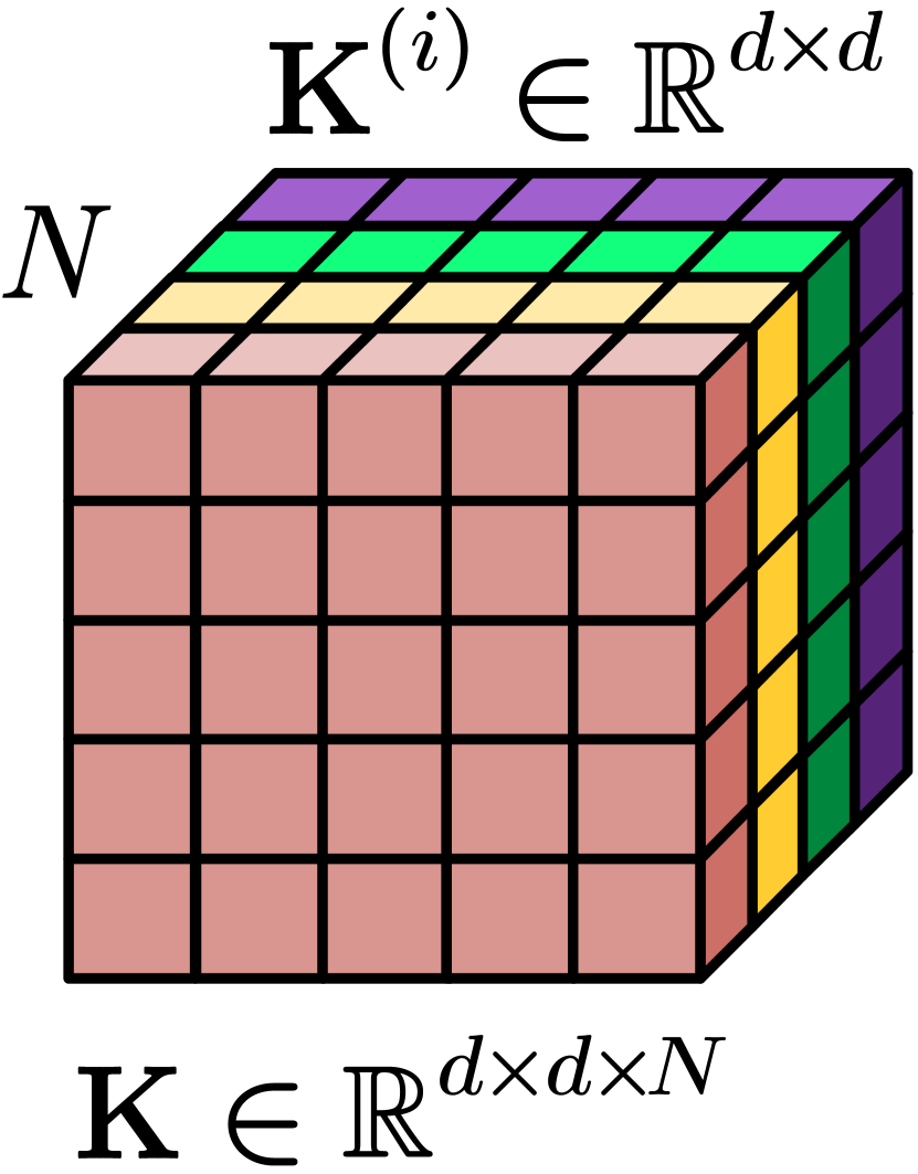
(a) Naive Method

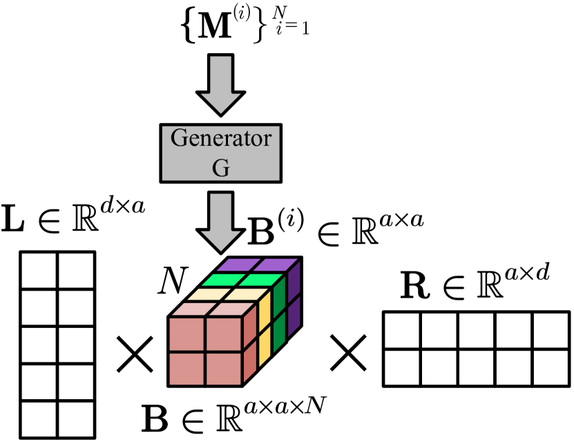
(b) Light-weight Method

Figure 5: Enabling Variable-Specific Projection Matrices. Different colors represent matrices for different variables and L and R are variable-agnostic, thus without colors. For the $i$-th variable, the naive method learns directly matrix $\textbf{K}^{(i)}$, while the light-weight method learns $\textbf{K}^{(i)}$ by $\textbf{L}\times\textbf{B}^{(i)}\times\textbf{R}$, where $\textbf{B}^{(i)}$ is generated by memory $\textbf{M}^{(i)}$ through a generator $\mathcal{G}$.

Method		Reformer		LogTrans		StemGNN		AGCRN		Informer		Autoformer		Triformer
	$F$	MSE	MAE	MSE	MAE	MSE	MAE	MSE	MAE	MSE	MAE	MSE	MAE	MSE	MAE
ETTh1	24	0.991	0.754	0.686	0.604	0.488	0.508	0.438	0.461	0.577	0.549	0.399	0.429	0.328	0.380
	48	1.313	0.906	0.766	0.757	0.473	0.505	0.488	0.486	0.685	0.625	0.405	0.439	0.359	0.401
	168	1.824	1.138	1.002	0.846	0.630	0.577	0.553	0.540	0.931	0.752	0.498	0.486	0.433	0.449
	336	2.117	1.280	1.362	0.952	0.658	0.598	0.611	0.566	1.128	0.873	0.500	0.480	0.487	0.475
	720	2.415	1.520	1.397	1.291	0.764	0.675	0.778	0.643	1.215	0.896	0.498	0.500	0.488	0.475
ETTm1	24	0.724	0.607	0.419	0.412	0.302	0.381	0.318	0.358	0.323	0.369	0.377	0.417	0.252	0.329
	48	1.098	0.777	0.507	0.583	0.382	0.436	0.426	0.429	0.494	0.503	0.429	0.442	0.275	0.337
	96	1.433	0.945	0.768	0.792	0.419	0.461	0.409	0.433	0.678	0.614	0.458	0.460	0.314	0.371
	288	1.820	1.094	1.462	1.320	0.522	0.518	0.545	0.531	1.056	0.786	0.632	0.526	0.385	0.427
	672	2.187	1.232	1.669	1.461	0.644	0.590	0.567	0.570	1.192	0.926	0.602	0.540	0.437	0.448
Weather	24	0.655	0.583	0.435	0.477	0.377	0.416	0.947	0.774	0.335	0.381	0.408	0.445	0.323	0.364
	48	0.729	0.666	0.426	0.495	0.438	0.467	0.948	0.777	0.395	0.459	0.475	0.487	0.390	0.429
	168	1.318	0.855	0.727	0.671	0.554	0.545	0.950	0.774	0.608	0.567	0.576	0.550	0.497	0.501
	336	1.930	1.167	0.754	0.670	0.598	0.573	0.946	0.772	0.702	0.620	0.593	0.558	0.538	0.531
	720	2.726	1.575	0.885	0.773	0.676	0.619	0.938	0.770	0.831	0.731	0.682	0.634	0.587	0.563
ECL	48	1.404	0.999	0.355	0.418	0.209	0.311	0.385	0.398	0.344	0.393	0.193	0.310	0.183	0.279
	168	1.515	1.069	0.368	0.432	0.265	0.355	0.481	0.509	0.368	0.424	0.223	0.334	0.182	0.288
	336	1.601	1.104	0.373	0.439	0.291	0.380	0.564	0.561	0.381	0.431	0.232	0.345	0.202	0.309
	720	2.009	1.170	0.409	0.454	0.317	0.400	0.725	0.678	0.406	0.443	0.257	0.361	0.251	0.335
	960	2.141	1.387	0.477	0.589	0.329	0.411	1.005	0.829	0.460	0.548	0.265	0.364	0.248	0.339

Table 2: Overall accuracy. Bold highlights the best results. Underline highlights the second best results.

Next, we propose to factorize a projection matrix, e.g., a Key matrix $\textbf{W}_{K}^{(i)}\in\mathbb{R}^{d\times d}$ into three matrices—a left variable-agnostic matrix $\textbf{L}_{K}\in\mathbb{R}^{d\times a}$, a middle variable-specific matrix $\textbf{B}^{(i)}\in\mathbb{R}^{a\times a}$, and a right variable-agnostic matrix $\textbf{R}_{K}\in\mathbb{R}^{a\times d}$. We intend to make the middle matrix compact, i.e., $a\ll d$, thus making the method light-weight.

The left and right matrices are variable-agnostic, thus being shared with all variables. Different variables have their own middle matrices $\{\textbf{B}^{(i)}\}_{i=1}^{N}$, thus making the middle matrices variable-specific. More specifically, the $i$-th variable’s middle matrix $\textbf{B}^{(i)}$ is generated from its memory $\textbf{M}^{(i)}$ using a generator $\mathcal{G}(\cdot)$, e.g., a 1-layer neural network. This step is also essential to reduce the number of parameters to be learned. Learning a full matrix B=$\{\textbf{B}^{(i)}\}_{i=1}^{N}$ directly requires $N{\cdot}a^{2}$ parameters. In contrast, when using a generator, it requires $N{\cdot}m$ for the memories, and an additional overhead of $m{\cdot}a^{2}$ for the generator.

In addition to the reduced parameter sizes, the factorization also contributes to improved accuracy (cf. Table 6 in Experiments). Since all variables’ time series share the variable-agnostic matrices L and R, they act as an implicit regularizer—the amount of combinations that can be produced using them is limited. It also facilitates implicit knowledge sharing among variables.

Equation 6 summarizes the generation of variable-specific Key and Value matrices $\textbf{W}_{K}^{(i)}$ and $\textbf{W}_{V}^{(i)}$, which replace $\textbf{W}_{K}$ and $\textbf{W}_{V}$ in Equation 3 to make Patch Attention variable-specific. We do not need the Query matrix as PA does not need it and employs the pseudo timestamp instead.

$$\begin{bmatrix}\textbf{W}_{K}^{(i)}\\ \textbf{W}_{V}^{(i)}\\ \end{bmatrix}=\begin{bmatrix}\textbf{L}_{K}\mathcal{G}(\textbf{M}^{(i)})\textbf{R}_{K}\\ \textbf{L}_{V}\mathcal{G}(\textbf{M}^{(i)})\textbf{R}_{V}\\ \end{bmatrix}$$ (6)

5 Experiments

We report on a comprehensive empirical study on four real-world, commonly used time series long term forecasting data sets to justify our design choices and demonstrate that Triformer outperforms the state-of-the-art methods.

5.1 Experimental Setup

Datasets: We consider four data sets and follow the setup from the-state-of-the-art method for long term forecasting Zhou et al. (2021).

ETT_h1, ETT_m1 (Electricity Transformer Temperature): ETT_h1 and ETT_m1 has observations every 15 minutes. Each observation consists of 6 power load features, making them 6-variate time series. To ensure fair comparisons with existing studies, following Zhou et al. (2021), the train/validation/test data cover 12/4/4 months.

ECL (Electricity Consumption Load) is a 321-variate time series, which records the hourly electricity consumption (Kwh) of 321 clients. Following Zhou et al. (2021), the train/validation/test data cover 15/3/4 months.

Weather is a 12-variate time series which record 12 different climate features, e.g., temperature, humidity, etc, from 1,600 U.S. locations. The data is collected hourly. Following Zhou et al. (2021), the train/validation/test data cover 28/10/10 months.

Forecasting Setups: We use historical $H$ timestamps to forecast the future $F$ timestamps. We vary $H$ and $F$ for different data sets, by following a commonly used long term forecasting setup Zhou et al. (2021). We vary $F$ progressively in {24, 48, 168, 336, 720, 960} for the hourly data sets ETT_h1, ECL, and Weather, corresponding to 1, 2, 7, 14, 30, and 40 days ahead; and we vary $F$ in {24, 48, 96, 288, 672} for ETT_m1 corresponding to 6, 12, 24, 72 and 168 hours ahead. We also vary the input historical timestamps $H$. For ETT_h1, Weather and ECL, we vary $H$ from {24, 48, 96, 168, 336, 720}, and from {24, 48, 96, 192, 288, 672} for ETT_m1. Following Zhou et al. (2021), for each $F$ value, we iterate all possible $H$ values and report the best values in Table 2.

Baselines: We select six recent and strong baselines from different categories shown in Table 1, including StemGNN Cao et al. (2020), AGCRN Bai et al. (2020), Informer Zhou et al. (2021), Reformer Kitaev et al. (2020), LogTrans Li et al. (2019), and Autoformer Wu et al. (2021).

Implementation Details: We use Adam optimizer with a static learning rate of $1e^{-4}$. We train the models for a maximum of 10 epoch, while utilizing early stopping with a patience of 3 and a batch size of 32. We set $d$=32, $m$=5, and $a$=5 as default values and we further study the effect of different values in the Appendix. Since the patch sizes are highly dependent on the input size $H$, we vary the patch sizes among 2, 3, 4, 6, 7, 12, and 24, and select the best patch sizes based on the validation set. We utilize the same positional embedding mechanism presented in Zhou et al. (2021). All models are trained/tested using a single NVIDIA V100 GPU.

The patch sizes are highly dependent on the input size $H$, we vary the patch sizes $S$ among {2, 3, 4, 6, 7, 12, 24} and vary the number of layers $L$ among {3, 4, 5}, and select the best patch sizes and the number of layers based on the validation set, which is shown in in Table 8. For instance, $(4,3,2,2)$ indicates that we employ a Triformer with 4-layer of patch attentions, where the patch sizes of the 1^st, 2^nd, 3^rd, and 4^th layers are 4, 3, 2, and 2, respectively.

$H$	$S$ and $L$
24	(4, 3, 2, 2)
48	(4, 3, 4)
96	(6, 4, 4)
168	(4, 7, 3, 2)
192	(6, 4, 4, 2)
288	(8, 4, 3, 3)
336	(7, 4, 3, 2, 2)
672	(7, 6, 4, 4)
720	(6, 6, 4)

Table 3: Patch Sizes and Number of Layers

Following Zhou et al. (2021), we consider 3 random training/validation setups, and the results are averaged over 3 runs. For all datasets, we perform standardization such that the mean of variable is 0 and the standard deviation is 1.

5.2 Experimental Results

Table 2 shows the overall accuracy. The results of Informer, Reformer and LogTrans are collected from Zhou et al. (2021). For AGCRN, StemGNN, and Autoformer we have used their original implementations which are publicly available. Triformer outperforms all baselines on all datasets. In most settings, AGCRN achieves better results when compared to the three attention based methods that are variable-agnostic Reformer, LogTrans and Informer. This highlights the needs of variable-specific modeling. Autoformer achieves the second best accuracy which highlights the importance of auto-correlation. Finally our proposed method, Triformer, achieves the best accuracy in all settings.

5.3 Experiments for Longer Sequences

We have performed an addition experiment on the ECL dataset in which we increase $H$ and $F$ to 1024 and 2048 respectively. We have selected the top two most competitive baselines in the form of Autoformer and Informer to compare our method against. The results can be seen in table 1 where Informer falls behind Triformer while Autoformer runs out of memory (OOM).

	Informer		Autoformer		Triformer
H/F	MSE	MSE	MSE	MAE	MSE	MAE
1,024	0.512	0.511	OOM	OOM	0.303	0.380
2,048	0.941	0.804	OOM	OOM	0.350	0.417

Table 1: Long time series, ECL.

5.4 Ablation Study

We perform an ablation study on the ECL dataset, as shown in Table 6. First, we remove the variable-specific modeling (VSM), where the same projection matrices are shared across all variables. We observe a significant loss of accuracy, which well justifies our design considerations to capture distinct temporal patterns of different variables. A shared parameter space for all variables fails to do so. Second, we replace the light-weight variable specific modeling by the naive way (cf. Figure 5(a)). We observe that the naive method is less accurate and incurs significant more parameters to be learned, which are well aligned with our design considerations. The generator $\mathcal{G}$ in Triformer takes very limited additional time to generate matrix B. Third, we do not stack multiple layers patch attentions but use only 1 layer of patch attentions. We observe a significant drop in accuracy, suggesting that the proposed multi-layer, triangular structure, is very effective. Fourth, we remove the multi-scale modeling such that only the top most layer’s output, rather than the outputs from all layers, is fed into the predictor. The accuracy drops significantly, which justifies our design choices of using multi-scale representations in the predictor. Finally, we remove the recurrent connections that connect two consecutive pseudo timestamps within PAs. The temporal information flow is thus broken, meaning that each patch is computed independently of the others. This results in sub-optimal accuracy. However, we note that the accuracy loss is much smaller than removing other components. One of the benefit of this variant is that this makes the computations of all PAs per layer fully parallelizable thus improving the running time.

	MSE	MAE	#Param	s/epoch
Triformer	0.183	0.279	347k	73.11
w/o VSM	0.215	0.273	303k	33.25
w Naive VSM	0.191	0.288	826k	63.81
w/o Stacking	0.203	0.295	258k	56.26
w/o Multiscale	0.266	0.352	285k	71.58
w/o Recurrent	0.191	0.290	346k	65.75

Table 5: Ablation Study, ECL.

Piece-by-Piece Ablation Study: We conduct a piece-by-piece ablation study (Table 6) to study the effects of the three main modules—patch attention (PA), triangular stacking (TS), and VSM. We consider (1) PA, a single PA layer; (2) PA+TS, triangular stacking of multiple PA layers; (3) PA+VSM, single PA layer with VSM; and (4) Triformer, i.e., PA+TS+VSM. In addition, to justify the need of recurrent connections (RC) in PA, we consider PA-RC, a single layer of PA without RC.

	MSE	MAE	#Param	s/epoch
PA	0.220	0.313	244k	26.26
PA-RC	0.223	0.314	224k	22.82
PA+TS	0.219	0.312	309k	30.31
PA+VSM	0.199	0.294	259k	48.92
Triformer	0.183	0.279	347k	73.11

Table 6: Piece-by-Piece Ablation Study, ECL.

Next, we study the effect of the proposed VSM when added to other related studies in the form of Informer Zhou et al. (2021). We can see from Table 7 that VSM generalize well, significantly increasing the accuracy of Informer.

	Informer		Informer+VSM		Triformer
F	MSE	MAE	MAE	MSE	MSE	MAE
48	0.344	0.393	0.274	0.367	0.183	0.279
168	0.368	0.424	0.284	0.376	0.182	0.288
336	0.381	0.431	0.294	0.386	0.202	0.309
720	0.406	0.443	0.316	0.401	0.251	0.335
960	0.460	0.548	0.317	0.396	0.248	0.339

Table 7: Effect of VSM, ECL.

5.5 Hyper-Parameter-Sensitivity Analysis

We study the impact of the most important hyper-parameters, including $d$, $m$, and $a$. We choose the ECL dataset to perform the experiments since it includes 321-variate (i.e., $N=321$) time series, which has the highest $N$ among all data sets.

In Table 8, (4, 4, 3) means that we use patch size 4, 4 and 3 for the 1^st, 2^nd, and 3^rd layers. The first two settings both have 3 layers and we observe similar accuracy, but (2, 6, 4) is slower and with more parameters because the first layer has a smaller patch size and thus more patches. This results in more pseudo timestamps being sent over to the next layer. Next, we observe (12, 2, 2) has a significant accuracy loss compared to the first two 3-layer settings, although the total number of parameters significant drops. When looking at the 2-layer settings, (8, 6) seems to achieve a good trade-off between accuracy and efficiency—it is not as accurate as the first two 3-layer variants but it is more than twice faster. To conclude, when using different patch sizes and layers, Triformer offers great flexibility to meet different needs on accuracy, efficiency, and parameter sizes.

	MSE	MAE	#Param	s/epoch
(4, 4, 3)	0.183	0.279	347k	73.11
(2, 6, 4)	0.181	0.276	423k	99.90
(12, 2, 2)	0.381	0.436	295k	37.32
(8, 6)	0.213	0.305	262k	35.16
(24, 2)	0.801	0.743	239k	27.63

Table 8: Sensitivity Analysis of Patch Size $S$, ECL

Impact of $d$: To study the impact of the size of the hidden representation $d$ used in the pseudo timestamps and projection matrices (cf. subsection “Linear Patch Attention” and “Variable-Specific Modeling”), we vary $d$ among {16, 32, 64}. The results are shown in Table 9. We observe that when $d$ is too small, e.g. $d=16$, the accuracy drops significantly, which indicates that a small $d$ is unable to capture well complex temporal patterns. In addition, the accuracy of $d=64$ is worse than that of $d=32$, which is a possible sign of over-fitting.

$d$	MSE	MAE
16	0.194	0.291
32	0.183	0.279
64	0.190	0.280

Table 9: Effect of $d$, ECL

Impact of $m$: To study the impact of $m$, i.e., the memory size of $\textbf{M}^{(i)}$ (cf. the section “Variable-Specific Modeling” and Figure 5 in the main paper), we ran multiple experiments in which we vary $m$ among {3, 5, 16, 32}. The results are shown in Table 10. We observe insignificant variations in terms of accuracy, which indicates the proposed method is insensitive w.r.t. the memory size.

$m$	MSE	MAE
3	0.185	0.281
5	0.183	0.279
16	0.186	0.285
32	0.188	0.284

Table 10: Effect of $m$, ECL

Impact of $a$: We study the impact of $a$, i.e., the size of the middle matrix $\textbf{B}^{(i)}$ (cf. the section “Variable-Specific Modeling” and Figure 5(b)). We vary $a$ among the following values {3, 5, 16, 32} and the results are shown in Table 11. We observe that when $a$ is too small, e.g. $a=3$, the accuracy drops significantly, which is understandable as the variable-specific matrix $\textbf{B}^{(i)}$ has a shape of $a\times a$, which may be too compact to capture sufficient variable-specific temporal patterns. In addition, we observe that $a=5$ is sufficient and increasing further $a$ to 32 does not contribute to improved accuracy.

$a$	MSE	MAE
3	0.191	0.288
5	0.183	0.279
16	0.184	0.280
32	0.186	0.281

Table 11: Effect of $a$ on ECL Dataset

Efficiency: Figure 6 shows the training runtime (seconds/epoch) of Triformer against other four baselines that show the second best accuracy in some data sets, i.e., Informer, AGCRN, StemGNN and Autoformer, as shown in Table 2. When varying $H$: (i) Triformer is faster than Informer and Autoformer, which is in accordance with the complexities of the two methods and also due to the efficient fully connected neural network based predictor. (ii) StemGNN increases faster as $H$ increases, while Triformer almost keeps steady. (iii) we observe that the recurrent based method AGCRN falls behind when compared with attention based methods, especially when the input time series is long, i.e., large $H$. When varying $F$, Triformer is the fastest in all settings. In addition, for inference time, all methods are less than 13.3 ms per inference, which are sufficiently efficient to support real-time forecasting.

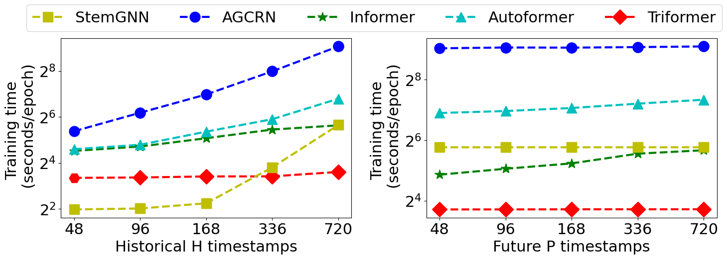
Figure 6: Training Runtime, seconds/epoch

5.5.1 Visualization of Learned Memories.

We visualize the learned memories $\textbf{M}^{(i)}$ to investigate whether they may capture distinct and the most prominent patterns of different variable’s time series. We select 8 time series from the ECL data sets, as shown in Figure 7. We use t-SNE Maaten and Hinton (2008) to compress each variable memory $\textbf{M}^{(i)}$ to a 2D point, which is also shown in Figure 7. We observe that the points are spread over the space, indicating that different time series have their own unique patterns. In addition, we observe that when the variables have similar temporal patterns, their learned memories are close by. For example, the time series of variables 6, 7, and 8 are similar, and their corresponding memories are also clustered together, i.e., in the right, top corner.

Figure 7: Visualization of the Learned Memories $\textbf{M}^{(i)}$ for different variables along with their time series.

6 Limitations and Possible Solutions

A limitation of the proposed Patch Attention PA is that the number of learnable parameters is related to forecasting settings. More specifically, a learnable query, i.e., a pseudo-timestamp, is needed per patch. For example, if we train the model on an input size $H=160$ with window size $S=10$, then we learn a total of $16$ pseudo-timestamps. If during testing, we want to change the input size to $H=200$, which requires $40$ pseudo-timestamps, making the already trained model inapplicable. Thus, this limitation prevents using Triformer in applications that need dynamic input lengths.

One possible solution is to introduce a generator to generate the learnable pseudo-timestamps from the index of the patch. By doing so, we only need to learn the parameters of the generator network, decoupling the number of patches from the number of learnable pseudo-timestamps, which leads to a more flexible model that addresses the limitation.

Furthermore, the proposed method cannot forecast different horizons once trained. To remedy this limitation, an encoder-decoder architecture could be used to replace the fully connected predictor, which enables forecasting in an auto-regressive manner.

7 Conclusion and Outlook

We propose Triformer, a triangular structure that employs novel patch attentions, which ensures linear complexity. Furthermore, we propose a light-weight method to generate variable-specific projection matrices which are tailored to capture distinct temporal patterns for each variable’s time series. Extensive experiments on four data sets show that our proposal outperforms other state-of-the-art methods for long sequence multivariate time series forecasting. In future work, it is of interest to explore different ways of supporting dynamic input lengths and to enhance model training using curriculum learning Yang et al. (2021, 2022).

References

- Bai et al. [2019] Lei Bai, Lina Yao, Salil S Kanhere, Zheng Yang, Jing Chu, and Xianzhi Wang. Passenger demand forecasting with multi-task convolutional recurrent neural networks. In PAKDD, pages 29–42, 2019.
- Bai et al. [2020] Lei Bai, Lina Yao, Can Li, Xianzhi Wang, and Can Wang. Adaptive graph convolutional recurrent network for traffic forecasting. In NeurIPS, pages 1–16, 2020.
- Beltagy et al. [2020] Iz Beltagy, Matthew E Peters, and Arman Cohan. Longformer: The long-document transformer. arXiv preprint arXiv:2004.05150, 2020.
- Campos et al. [2022] David Campos, Tung Kieu, Chenjuan Guo, Feiteng Huang, Kai Zheng, Bin Yang, and Christian S. Jensen. Unsupervised time series outlier detection with diversity-driven convolutional ensembles. Proc. VLDB Endow., 15(3):611–623, 2022.
- Cao et al. [2020] Defu Cao, Yujing Wang, Juanyong Duan, Ce Zhang, Xia Zhu, Congrui Huang, Yunhai Tong, Bixiong Xu, Jing Bai, Jie Tong, and Qi Zhang. Spectral temporal graph neural network for multivariate time-series forecasting. In NeurIPS, pages 17766–17778, 2020.
- Cirstea et al. [2019] Razvan-Gabriel Cirstea, Bin Yang, and Chenjuan Guo. Graph attention recurrent neural networks for correlated time series forecasting. In MileTS19@KDD, 2019.
- Cirstea et al. [2021] Razvan-Gabriel Cirstea, Tung Kieu, Chenjuan Guo, Bin Yang, and Sinno Jialin Pan. EnhanceNet: Plugin neural networks for enhancing correlated time series forecasting. In ICDE, pages 1739–1750, 2021.
- Cirstea et al. [2022] Razvan-Gabriel Cirstea, Bin Yang, Chenjuan Guo, Tung Kieu, and Shirui Pan. Towards spatio-temporal aware traffic time series forecasting. In ICDE, 2022.
- Dai et al. [2020] Zihang Dai, Guokun Lai, Yiming Yang, and Quoc V Le. Funnel-transformer: Filtering out sequential redundancy for efficient language processing. In NeurIPS, 2020.
- Dauphin et al. [2017] Yann N Dauphin, Angela Fan, Michael Auli, and David Grangier. Language modeling with gated convolutional networks. In ICML, pages 933–941, 2017.
- Dosovitskiy et al. [2021] Alexey Dosovitskiy, Lucas Beyer, Alexander Kolesnikov, Dirk Weissenborn, Xiaohua Zhai, Thomas Unterthiner, Mostafa Dehghani, Matthias Minderer, Georg Heigold, Sylvain Gelly, et al. An image is worth 16x16 words: Transformers for image recognition at scale. In ICLR, 2021.
- Guo et al. [2020] Chenjuan Guo, Bin Yang, Jilin Hu, Christian S. Jensen, and Lu Chen. Context-aware, preference-based vehicle routing. VLDB J., 29(5):1149–1170, 2020.
- Hochreiter and Schmidhuber [1997] Sepp Hochreiter and Jürgen Schmidhuber. Long short-term memory. Neural Comput., 9(8):1735–1780, 1997.
- Hu et al. [2020] Jilin Hu, Bin Yang, Chenjuan Guo, Christian S. Jensen, and Hui Xiong. Stochastic origin-destination matrix forecasting using dual-stage graph convolutional, recurrent neural networks. In ICDE, pages 1417–1428, 2020.
- Katharopoulos et al. [2020] Angelos Katharopoulos, Apoorv Vyas, Nikolaos Pappas, and François Fleuret. Transformers are rnns: Fast autoregressive transformers with linear attention. In International Conference on Machine Learning, pages 5156–5165. PMLR, 2020.
- Khandelwal et al. [2018] Urvashi Khandelwal, He He, Peng Qi, and Dan Jurafsky. Sharp nearby, fuzzy far away: How neural language models use context. ACL, pages 284–294, 2018.
- Kieu et al. [2022a] Tung Kieu, Bin Yang, Chenjuan Guo, Razvan-Gabriel Cirstea, Yan Zhao, Yale Song, and Christian S. Jensen. Anomaly detection in time series with robust variational quasi-recurrent autoencoders. In ICDE, 2022.
- Kieu et al. [2022b] Tung Kieu, Bin Yang, Chenjuan Guo, Christian S. Jensen, Yan Zhao, Feiteng Huang, and Kai Zheng. Robust and explainable autoencoders for time series outlier detection. In ICDE, 2022.
- Kitaev et al. [2020] Nikita Kitaev, Lukasz Kaiser, and Anselm Levskaya. Reformer: The efficient transformer. ICLR, pages 1–12, 2020.
- Li et al. [2018] Yaguang Li, Rose Yu, Cyrus Shahabi, and Yan Liu. Diffusion convolutional recurrent neural network: Data-driven traffic forecasting. In ICLR, pages 1–16, 2018.
- Li et al. [2019] Shiyang Li, Xiaoyong Jin, Yao Xuan, Xiyou Zhou, Wenhu Chen, Yu-Xiang Wang, and Xifeng Yan. Enhancing the locality and breaking the memory bottleneck of transformer on time series forecasting. In NeurIPS, pages 5244–5254, 2019.
- Liu et al. [2018] Huiping Liu, Cheqing Jin, Bin Yang, and Aoying Zhou. Finding top-k optimal sequenced routes. In ICDE, pages 569–580, 2018.
- Maaten and Hinton [2008] Laurens van der Maaten and Geoffrey Hinton. Visualizing data using t-SNE. J. Mach. Learn. Res., 9(11):2579–2605, 2008.
- Pan et al. [2019] Zheyi Pan, Yuxuan Liang, Weifeng Wang, Yong Yu, Yu Zheng, and Junbo Zhang. Urban traffic prediction from spatio-temporal data using deep meta learning. In SIGKDD, pages 1720–1730, 2019.
- Pan et al. [2021] Zizheng Pan, Bohan Zhuang, Jing Liu, Haoyu He, and Jianfei Cai. Scalable vision transformers with hierarchical pooling. ICCV, 2021.
- Pappagari et al. [2019] Raghavendra Pappagari, Piotr Zelasko, Jesús Villalba, Yishay Carmiel, and Najim Dehak. Hierarchical transformers for long document classification. In ASRU, pages 838–844, 2019.
- Pedersen et al. [2020a] Simon Aagaard Pedersen, Bin Yang, and Christian S. Jensen. Anytime stochastic routing with hybrid learning. Proc. VLDB Endow., 13(9):1555–1567, 2020.
- Pedersen et al. [2020b] Simon Aagaard Pedersen, Bin Yang, and Christian S. Jensen. Fast stochastic routing under time-varying uncertainty. VLDB J., 29(4):819–839, 2020.
- Qin et al. [2017] Yao Qin, Dongjin Song, Haifeng Chen, Wei Cheng, Guofei Jiang, and Garrison Cottrell. A dual-stage attention-based recurrent neural network for time series prediction. IJCAI, pages 2627–2633, 2017.
- Seo et al. [2018] Youngjoo Seo, Michaël Defferrard, Pierre Vandergheynst, and Xavier Bresson. Structured sequence modeling with graph convolutional recurrent networks. In ICONIP, pages 362–373, 2018.
- Stoller et al. [2020] Daniel Stoller, Mi Tian, Sebastian Ewert, and Simon Dixon. Seq-u-net: A one-dimensional causal u-net for efficient sequence modelling. In IJCAI, pages 2893–2900, 2020.
- Vaswani et al. [2017] Ashish Vaswani, Noam Shazeer, Niki Parmar, Jakob Uszkoreit, Llion Jones, Aidan N. Gomez, Lukasz Kaiser, and Illia Polosukhin. Attention is all you need. NIPS, page 6000–6010, 2017.
- Wang et al. [2020] Sinong Wang, Belinda Z Li, Madian Khabsa, Han Fang, and Hao Ma. Linformer: Self-attention with linear complexity. arXiv preprint arXiv:2006.04768, 2020.
- Wu et al. [2019] Zonghan Wu, Shirui Pan, Guodong Long, Jing Jiang, and Chengqi Zhang. Graph wavenet for deep spatial-temporal graph modeling. In IJCAI, pages 1907–1913, 2019.
- Wu et al. [2020] Zonghan Wu, Shirui Pan, Guodong Long, Jing Jiang, Xiaojun Chang, and Chengqi Zhang. Connecting the dots: Multivariate time series forecasting with graph neural networks. In SIGKDD, pages 753–763, 2020.
- Wu et al. [2021] Haixu Wu, Jiehui Xu, Jianmin Wang, and Mingsheng Long. Autoformer: Decomposition transformers with auto-correlation for long-term series forecasting. In NIPS, 2021.
- Wu et al. [2022] Xinle Wu, Dalin Zhang, Chenjuan Guo, Chaoyang He, Bin Yang, and Christian S. Jensen. AutoCTS: Automated correlated time series forecasting. Proc. VLDB Endow., 15(4):971–983, 2022.
- Yang et al. [2021] Sean Bin Yang, Chenjuan Guo, Jilin Hu, Jian Tang, and Bin Yang. Unsupervised path representation learning with curriculum negative sampling. In IJCAI, pages 3286–3292, 2021.
- Yang et al. [2022] Sean Bin Yang, Chenjuan Guo, Jilin Hu, Bin Yang, Jian Tang, and Christian S. Jensen. Temporal path representation learning with weakly-supervised contrastive curriculum learning. In ICDE, 2022.
- Zhou et al. [2021] Haoyi Zhou, Shanghang Zhang, Jieqi Peng, Shuai Zhang, Jianxin Li, Hui Xiong, and Wancai Zhang. Informer: Beyond efficient transformer for long sequence time-series forecasting. In AAAI, pages 11106–11115, 2021.