Probabilistic Permutation Graph Search:
Black-Box Optimization for Fairness in Ranking

Abstract.

There are several measures for fairness in ranking, based on different underlying assumptions and perspectives. Plackett-Luce (PL) optimization with the REINFORCE algorithm can be used for optimizing black-box objective functions over permutations. In particular, it can be used for optimizing fairness measures. However, though effective for queries with a moderate number of repeating sessions, PL optimization has room for improvement for queries with a small number of repeating sessions.

In this paper, we present a novel way of representing permutation distributions, based on the notion of permutation graphs. Similar to PL, our distribution representation, called  probabilistic permutation graph (PPG), can be used for black-box optimization of fairness. Different from PL, where pointwise logits are used as the distribution parameters, in PPG pairwise inversion probabilities together with a reference permutation construct the distribution. As such, the reference permutation can be set to the best sampled permutation regarding the objective function, making PPG suitable for both deterministic and stochastic rankings. Our experiments show that PPG, while comparable to PL for larger session repetitions (i.e., stochastic ranking), improves over PL for optimizing fairness metrics for queries with one session (i.e., deterministic ranking). Additionally, when accurate utility estimations are available, e.g., in tabular models, the performance of PPG in fairness optimization is significantly boosted compared to lower quality utility estimations from a learning to rank model, leading to a large performance gap with PL. Finally, the pairwise probabilities make it possible to impose pairwise constraints such as “item $d_{1}$ should always be ranked higher than item $d_{2}$.” Such constraints can be used to simultaneously optimize the fairness metric and control another objective such as ranking performance.

1. Introduction

Several fairness measures are being considered in the search and recommendation literature. Different measures have been proposed based on different definitions of fairness, aimed at different environments. For instance, Singh and Joachims (2018) consider the disparate treatment ratio (DTR), which ensures equity of exposure: each group should get exposed proportional to their utility. DTR for group fairness can be used for deterministic rankers, which produce one ranking per query, as well as stochastic rankers, with different randomly sampled rankings per query. It also makes no assumptions about the utility values of the ranked items. In contrast, the  expected exposure loss (EEL) is based on the premise that groups (or individuals) with the same relevance level should have equal expected exposures (Diaz et al., 2020). By definition, EEL should be used for stochastic rankers. It is also assumed in EEL that the relevance levels have discrete values.

Optimizing fairness measures. The goal of this paper is not to list and compare different fairness definitions; much has already been written about this (Verma and Rubin, 2018; Raj et al., 2020). Neither do we want to unify different fairness measures, since they deal with different aspects of fairness, and more importantly, it has been shown that there is an inherent trade-off between some fairness conditions (Kleinberg et al., 2017), which makes it impossible to have a unified fairness measure. What we aim to accomplish is to provide a general framework that can be used for optimizing any fairness measure.

We focus on post-processing methods for fairness and assume that the utility value of the items is given, either from external sources such as unbiased clicks or an estimate computed by a learning to rank (LTR) model. In order to remain general, the framework should work with black-box access to the function that evaluates ranking fairness. Optimization of fairness in ranking is a special case of permutation optimization, and reinforcement learning (RL) is usually the default paradigm for combinatorial optimization: A model-free policy-based RL can be used for permutation optimization (Bello et al., 2016). Using the well-known REINFORCE algorithm (Williams, 1992), and sampling from a PL distribution, it is possible to optimize any fairness objective function on permutations (Singh and Joachims, 2019).

A PL distribution with the REINFORCE algorithm works very well for optimizing stochastic ranking evaluation metrics such as EEL. However, there are two directions in which PL-based optimization has room for improvement. First, when the number of repeating sessions for a query is very small, the high variance of PL (Gadetsky et al., 2020) leads to sub-optimal results. Second, when an accurate estimate of the utilities is available, the solutions obtained from PL are only slightly improved over the case of noisy utility values. The first case has practical importance, as it is desirable to have a good fairness solution as soon as possible, before there are a large number of repeating sessions, i.e., a method that provides fair solutions both for deterministic and stochastic rankings. The second case has both theoretical and practical importance. From a theoretical point of view, since fairness measures usually depend on utility values, noise in utility estimates propagates into the fairness optimization, whereas with accurate utility values, the performance of the fairness optimizer is isolated and not affected by noise from utility values. This gives a more accurate comparison between different optimization algorithms. From a practical point of view, given enough historical sessions, unbiased and accurate estimates of utility can be obtained from clicks (Joachims et al., 2017; Vardasbi et al., 2021; Zoghi et al., 2016; Li et al., 2020). For instance, extremely high performance rankings can be achieved from tabular models in practice (Sorokina and Cantu-Paz, 2016). We expect to observe a boost in fairness optimization when noisy estimates are replaced with unbiased low noise estimates of utility.

Black-box permutation optimization. To bridge the performance gap left by PL in the above two cases, we propose a novel permutation distribution for black-box permutation optimization with the REINFORCE algorithm. Our permutation distribution is based on the notion of permutation graphs (Dushnik and Miller, 1941). A permutation graph is a graph whose nodes are the items in a ranked list, and whose edges represent inversions in a permutation over the ranked list. We refer to the initial permutation of the ranked list as the reference permutation. Two examples of permutation graphs are given in Fig. 1. In the left graph, over the reference permutation of $[d_{1},d_{2},d_{3},d_{4}]$, $d_{1}$ is moved from the first position to the third, causing two inversions $(d_{1},d_{2})$ and $(d_{1},d_{3})$. In the right graph, over the reference permutation of $[d_{3},d_{2},d_{4},d_{1}]$, $d_{1}$ is brought forward, and $d_{3}$ is swapped with $d_{2}$, causing a total of four inversions, as can be seen in the graph.

$[d_{1},d_{2},d_{3},d_{4}]\rightarrow[d_{2},d_{3},d_{1},d_{4}]$	$[d_{3},d_{2},d_{4},d_{1}]\rightarrow[d_{1},d_{2},d_{3},d_{4}]$

Figure 1. Examples of permutation graphs.

Building on permutation graphs, we define probabilistic permutation graph (PPG) as a permutation distribution from which the REINFORCE algorithm can sample. Roughly speaking, PPG is a weighted complete graph, whose edge weights are the probabilities of inverting the two endpoints in a permutation. Unlike PL, in which pointwise logits are used as distribution parameters, PPG is constructed from a reference permutation together with pairwise inversion probabilities. The reference permutation in PPG helps in deterministic scenarios, as it can be set to the best permutation sampled during the REINFORCE algorithm. This is not possible for a PL distribution, as the deterministic permutation of PL comes from sorting the items based on their logits and such a permutation is not necessarily the best sampled permutation during training.

In addition to PPG’s gain over PL due to its reference permutation in deterministic as well as accurate relevance estimation scenarios, the pairwise inversion probabilities give PPG another useful property that PL lacks. In PPG, pairwise constraints can be added during optimization, without any additional computational overhead: it is enough to set some edge weights to non-trainable parameters. For example, the constraint of “item $d_{1}$ should always be ranked higher than item $d_{2}$” can be added by setting to zero the weight of the $(d_{1},d_{2})$ edge. Business related, time-aware, or context-aware pairwise constraints can be thought of, all of which are easily handled by PPG (see Sec. 3.4).

Our fairness optimization method is a post-processing method that acts on lists of items, ranked based on utility. Compared to in-processing methods, such as (Singh and Joachims, 2019), a post-processing method allows for richer dynamics, in the sense that having the fairness optimizer separate from the ranker, makes any change on the fairness side independent of the ranking side. For example, with a post-processing method, if the sensitive groups of attention change over time, either by adding new sensitive features to the existing ones or replacing them, there is no need to re-train the ranker with a new set of group labels. Our black-box fairness optimization method even adds to this flexibility, as the objective fairness measure itself is allowed to change over time or in different contexts. Adding to this flexibility, while in-processing fairness optimization methods are an option in feature-based ranking models, they simply cannot be used in tabular models where best rankings are memorized.

Our contributions. Our contributions are listed below:

1. We define  probabilistic permutation graph (PPG), a novel permutation distribution.

2. We present PPG search as a general framework for optimizing fairness in ranking. Our method is general in the sense that it works with black-box access to the objective function. As such, PPG search can be used in contexts beyond fairness and diversity, to find a permutation that optimizes a general objective function.

3. We experimentally show the effectiveness of PPG search on two popular objective functions, EEL and DTR, and various public datasets by comparing its performance with state-of-the-art methods for optimizing fairness.

4. We experimentally verify the effect of pairwise constraints on controlling the ranking performance while optimizing for fairness.

2. Background and Related Work

Fairness. Widely used ranking algorithms at the core of many online systems such as search engines and recommender systems raise fairness considerations, since these algorithms can directly control the exposure each item receives and potentially have societal impacts (Baeza-Yates, 2018).

Similar to other areas of machine learning, various approaches have been proposed to evaluate fairness in ranking. Zehlike et al. (2021) distinguish two lines of work based on how fairness is measured for a ranking policy: probability-based approaches determine the probability that a given ranking is generated by a fair policy (Yang and Stoyanovich, 2017; Zehlike et al., 2017; Asudeh et al., 2019; Celis et al., 2020, 2018; Geyik et al., 2019; Stoyanovich et al., 2018), while exposure-based methods aim to ensure that the expected exposure is fairly distributed among items (individual fairness), or item groups (group fairness) (Biega et al., 2018; Mehrotra et al., 2018; Morik et al., 2020; Sapiezynski et al., 2019; Singh and Joachims, 2018, 2019; Yadav et al., 2019; Diaz et al., 2020; Heuss et al., 2022; Sarvi et al., 2021).

From the methods belonging to the second category, many have followed the concept of demographic parity, which enforces a proportional allocation of exposure between groups (Yang and Stoyanovich, 2017; Celis et al., 2018; Geyik et al., 2019; Zehlike et al., 2017). This approach to fairness does not consider merit and only takes into account the group size. On the other hand, disparate treatment is a merit-based approach to fair ranking proposed in (Singh and Joachims, 2018) which makes exposure allocation dependent on the merit of each group. They developed a framework which allows for other forms of fairness definitions that can be formulated as linear constraints.

Methods introduced in these publications are dependent on their notion of fairness. However, fairness goals can be application specific. In this work, we propose a black-box optimization method for fairness in ranking that is able to optimize a ranking policy w.r.t. any arbitrary fairness definition.

Gradient estimators for permutations. The group of all permutations of size $n$ is called the symmetric group and is denoted by $S_{n}$. Permutation optimization can be stated as follows:

$$\min f(b),\quad b\in S_{n},$$

where $f:S_{n}\rightarrow\mathbb{R}$ can be any general function on permutations. For this combinatorial optimization problem, the gradient solution is not as clear as continuous differentiable optimization. Instead, a policy-based RL approach can be used to optimize the expectation of $f(b)$ over a differentiable probability distribution $P(b\mid\theta)$, represented by a vector of continuous parameters $\theta$ (Berny, 2000):

(1) $$F(\theta)=\mathbb{E}_{P(b\mid\theta)}\left[f(b)\right].$$

$F(\theta)$ is optimized when $P(b\mid\theta)$ is totally concentrated on $b^{*}$, the optimum solution of $f(b)$. For Eq. (1), the REINFORCE estimator (Williams, 1992) can be used:

(2) $$\nabla_{\theta}F(\theta)=\mathbb{E}_{P(b\mid\theta)}\left[f(b)\cdot\nabla_{\theta}\log P\left(b\mid\theta\right)\right].$$

Finally, since $S_{n}$ is exponentially large, the expectation in Eq. (2) can be estimated through  Monte-Carlo (MC) sampling:

(3) $$\nabla_{\theta}F(\theta)\approx\frac{1}{\lambda}\sum_{i=1}^{\lambda}{f(b_{i})\cdot\nabla_{\theta}\log P\left(b_{i}\mid\theta\right)},$$

where $b_{1},\dots,b_{\lambda}\in S_{n}$ are samples drawn from $P(b\mid\theta)$.

It remains to discuss the probability distribution on $S_{n}$. For a thorough exploration of probability distributions for permutations we refer the reader to (Fligner and Verducci, 1988). The PL model (Luce, 1959; Plackett, 1975) is by far the most widely used permutation distribution in the REINFORCE algorithm, both in general permutation optimization (Gadetsky et al., 2020) and the fairness literature (Singh and Joachims, 2019; Oosterhuis, 2021). PL is represented by a parameter vector $\theta\in\mathbb{R}^{n}$, and the probability of a permutation $b=[b_{1},\dots,b_{n}]\in S_{n}$ under PL is calculated as:

(4) $$P(b\mid\theta)=\prod_{i=1}^{n-1}\frac{\theta_{b_{i}}}{\sum_{j=i}^{n}\theta_{b_{j}}}.$$

Sampling from PL and estimating the log derivative of the probability $P(b\mid\theta)$ is usually done using the Gumbel Softmax trick (Gumbel, 1954; Maddison et al., 2014).

In this work, we use the REINFORCE algorithm but with our novel PPG distribution instead of PL.

Tabular search. In practice, not all the queries are served with a feature-based LTR model. Tabular models usually achieve optimal performance for head and torso queries for which enough user interactions are available (Lagrée et al., 2016). In particular, underperforming torso queries are given to the tabular models for a better memorized ranking (Zoghi et al., 2016; Sorokina and Cantu-Paz, 2016; Grainger, 2021; Mavridis et al., 2020; Trotman et al., 2017). The online LTR literature is filled with methods for tabular model optimization (Katariya et al., 2016; Lagrée et al., 2016; Li et al., 2020). As tabular models are not limited by the capacity of the LTR model, they usually converge to extremely high ranking performance (Zoghi et al., 2016; Oosterhuis and de Rijke, 2021).

This work relates to tabular search by exploiting its results as a use case. We show in our experiments that, given accurate estimates of utility measures of the items, e.g., their relevance labels, our proposed method for fairness optimization performs significantly better than state-of-the-art fairness optimizers. Tabular models are practical and important evidence to show that the availability of accurate relevance estimates is not just hypothetical.

3. Probabilistic Permutation Graph Search

Given a list of items $D$, together with a black-box objective function $f:S_{n}\rightarrow\mathbb{R}$ that can be queried for every permutation of $D$, our goal is to find a distribution over permutations that optimizes $f$. We assume that the utility of items, e.g., their relevance level, is given, or an estimate of the utility is obtainable using a  learning to rank (LTR) model. Therefore, our task is to post-process a ranked list and output a permutation, or a sequence of permutations, that optimize the given objective function. To do so, we use the REINFORCE algorithm to search the permutation space and update the PPG distribution parameters. Below, we first formally define PPG and provide a log derivative formula for the PPG distribution. After that, we propose a method for efficiently sampling from the PPG distribution. Finally, we discuss pairwise constraints, including practical examples.

3.1. PPG distributions

We define PPG to be a probabilistic graph from which permutation graphs are sampled.

Definition 3.1 ( probabilistic permutation graph (PPG)).

Given a list of items $D$ and a reference permutation $\pi_{0}$ on $D$, a PPG corresponding to $\pi_{0}$ is a weighted complete graph $G=(D,E,w)$, whose edges are weighted by a probability value obtained from $w:E\rightarrow[0,1]$. For each edge $e\in E$, its weight $w(e)$ indicates the Bernoulli sampling probability that $e$ is included in a permutation graph over $\pi_{0}$ sampled from $G$.

In what follows, we write $e_{ij}$ for the edge $(d_{i},d_{j})$ and $w_{e_{ij}}$ for its weight (or $w_{ij}$ when no confusion is possible). According to the above definition, PPG represents a permutation distribution. To sample a permutation from a given PPG, a Bernoulli sampling process is run on the edges of $G$ with their corresponding weights. Suppose that, after edge sampling, $E_{\pi}\subset E$ is the set of edges that are selected (i.e., positively sampled) by the sampler and $E\setminus E_{\pi}$ is the set of remaining, left out edges (i.e., negatively sampled). The probability of this outcome is calculated as:

(5) $$P(E_{\pi}\mid w)=\prod_{e\in E_{\pi}}w_{e}\cdot\prod_{e\in E\setminus E_{\pi}}\bigl{(}1-w_{e}\bigr{)}.$$

Now, we notice that the set of all permutation graphs over a list of items $D$ is only a small subset of all possible graphs. This means that $E_{\pi}$ may not correspond to the edges of a valid permutation graph. If that happens, i.e., if the graph constructed from the $E_{\pi}$ edge set is not a permutation graph, we drop $E_{\pi}$ and repeat the sampling process until we find a valid permutation graph. Checking if a given graph is a permutation graph or not is possible in linear time (McConnell and Spinrad, 1999). We write $\mathcal{P}$ for the space of all permutation graphs. Then, the probability that a randomly sampled graph from $G$ is a permutation graph can be computed in theory by:

(6) $$\rho=\sum_{E_{\pi}\in\mathcal{P}}P(E_{\pi}\mid w).$$

Note that in practice, computing $\rho$ requires an exponential $n!$ number of computations and, hence, is not feasible. We will come back to this point in Appendix A below. Using $\rho$, the permutation probability mass can be written as:

(7) $$P(E_{\pi}\mid w,E_{\pi}\in\mathcal{P})=\frac{1}{\rho}\prod_{e\in E_{\pi}}w_{e}\cdot\prod_{e\in E\setminus E_{\pi}}\bigl{(}1-w_{e}\bigr{)}.$$

It is not hard to show that repeatedly sampling graphs until we sample a valid permutation graph will lead to the conditional probability distribution of Eq. (7). We interchangeably use $E_{\pi}\in\mathcal{P}$ for both the positively sampled edges of the permutation graph, and the permutation corresponding to the graph.

To work with the REINFORCE algorithm (Sec. 2), we need to compute the log derivative of the probability distribution of PPG. In what follows we assume that $E_{\pi}\in\mathcal{P}$ and drop the conditions from our notation for brevity. We start by using Eq. (7) and taking the log derivative as follows:

(8) $$\begin{split}\frac{\partial\log P(E_{\pi})}{\partial w_{e}}={}&\frac{\partial}{\partial w_{e}}\log\left(\prod_{e\in E_{\pi}}w_{e}\cdot\prod_{e\in E\setminus E_{\pi}}\bigl{(}1-w_{e}\bigr{)}\right)\\ &-\frac{\partial}{\partial w_{e}}\log\rho\\ ={}&{\frac{\mathbb{I}\bigl{(}e\in E_{\pi}\bigr{)}-w_{e}}{w_{e}\cdot\bigl{(}1-w_{e}\bigr{)}}}-{\frac{1}{\rho}\frac{\partial\rho}{\partial w_{e}}}.\end{split}$$

where $\mathbb{I}(\cdot)$ is the indicator function. In Appendix A we show the second term can be ignored to obtain the following approximation:

(9) $$\frac{\partial\log P(E_{\pi})}{\partial w_{e}}\approx\frac{\mathbb{I}\bigl{(}e\in E_{\pi}\bigr{)}-w_{e}}{w_{e}\cdot\bigl{(}1-w_{e}\bigr{)}}.$$

So far, we have defined the PPG and provided the log derivative of its probability distribution. However, repeatedly dropping the sampled graphs until a valid permutation graph is found, is not efficient. Next, we present an efficient method for sampling permutations from the PPG distribution.

3.2. Efficient sampling of permutation graphs

In order to avoid redundantly sampling non-permutation graphs from a PPG, we propose a divide and conquer approach for efficiently constructing a valid permutation graph. The idea is to divide the list of items into two sub-lists, obtain a permutation on each of the sub-lists by recursively sampling from the given PPG, and merge the two sampled sub-lists into a single permuted list. Below, we discuss our merge sampling method in more detail, but first, let us give an example to illustrate the general idea.

Case 1:		Case 2:		Case 3:
$[\underline{d_{2},d_{1}},d_{3},d_{4}]$		$[d_{2},\underline{d_{3},d_{1}},d_{4}]$		$[d_{2},d_{3},\underline{d_{4},d_{1}}]$

Figure 2. Different cases in Example 3.2. Dotted lines show the impossible-to-be-selected edges due to the position of $d_{1}$ in the bottom sub-list.

Example 0.

Suppose a reference permutation $[d_{1},d_{2},d_{3},d_{4}]$ and a PPG are given. In order to sample a permutation, we proceed as follows:

1. Divide. We divide the list into two sub-lists $[d_{1},d_{2}]$ and $[d_{3},d_{4}]$.

2. Sample sub-lists. Each sub-list is sampled independently according to PPG. Here, each pair of $[d_{1},d_{2}]$ and $[d_{3},d_{4}]$ are swapped with a probability equal to their weight, i.e., $w_{12}$ and $w_{34}$. Suppose only the first pair is swapped $[d_{1},d_{2}]\rightarrow[d_{2},d_{1}]$.

3. Merge. Finally, we merge $[d_{2},d_{1}]$ and $[d_{3},d_{4}]$. In doing so, we keep the order of items in each sub-list unchanged, i.e., no new edges are added between the items of the same sub-list. We start from the last item of the first sub-list, $d_{1}$. $d_{1}$ can go to three possible positions as depicted in Fig. 2: (Case 1) Before $d_{3}$, so $e_{13}$ is negatively sampled. In this case, since the order of the first sub-list should remain unchanged, $d_{2}$ has only one possible position. (Case 2) Between $d_{3}$ and $d_{4}$, so only $e_{13}$ is positively sampled. In this case, $d_{2}$ has two possible positions: before and after $d_{3}$. (Case 3) After $d_{4}$, so both $e_{13}$ and $e_{14}$ are positively sampled and $d_{2}$ has three possible positions. These three possibilities are tested sequentially. First, we sample $e_{13}$. If it is not selected, it means $d_{1}$ should remain before $d_{3}$ and we are done (Case 1). Otherwise, $d_{1}$ should go after $d_{3}$. Then, we sample $e_{14}$ and stop if it is not selected (Case 2). Finally, if $e_{14}$ is also selected, we have case 3. After $d_{1}$ has been merged, we repeat the above process for merging $d_{2}$.

4. Probability correction. If $e_{13}$ is negatively sampled, neither $e_{14}$ or $e_{23}$ can be sampled (Fig. 2, Case 1). Therefore, when sampling $e_{13}$, we have to account for the impossible outcome of not selecting $e_{13}$ but selecting at least one of $e_{14}$ or $e_{23}$. The probability of this event is calculated as:

   $$q_{13}=(1-w_{13})(w_{14}+w_{23}-w_{14}w_{23}).$$

   The sum of possible outcomes would then be equal to $1-q_{13}$ and the sampling probability of $e_{13}$ should be corrected by $w_{13}/\bigl{(}1-q_{13}\bigr{)}$. Similar arguments can be given for Case 2, where $e_{13}$ is positively sampled. Similarly, not selecting $e_{14}$ but selecting $e_{24}$ is impossible. So, sampling of $e_{14}$ should be done by a probability equal to $w_{14}/\bigl{(}1-q_{14}\bigr{)}$, where $q_{14}=(1-w_{14})w_{24}$. $\square$

In the above example, we saw the simplest case of merging two sub-lists of size two. More generally, assume we want to merge two permuted sub-lists $[d_{1},\dots,d_{T}]$ and $[d_{T+1},\dots,d_{n}]$. Here we re-indexed the items to simplify the notation. We start by merging the last item from the top sub-list $d_{T}$ into the bottom sub-list. Assume $d_{t+1}$ from the top sub-list is merged just after $d_{b}$ in the bottom sub-list. Now, for merging $d_{t}$, we know that it should be placed before $d_{t+1}$, meaning that at most it can be inverted with $d_{b}$, but not any item after that in the bottom sub-list. Starting from $d_{T+1}$ on the bottom sub-list, we sample the inversions using the corrected probabilities and stop as soon as one inversion was sampled negatively. Assume the inversions of $d_{t}$ with $d_{T+1},\dots,d_{i-1}$ were positively sampled and we want to sample the inversion with $d_{i}$. There are two independent impossible outcomes: $e_{ti}$ is sampled negatively, but ($A$) at least one of the $e_{tj}$ for $i<j\leq b$ is sampled positively; or ($B$) at least one of the $e_{t^{\prime}i}$ for $t^{\prime}<t$ is sampled positively. The probability of these impossibilities can easily be calculated. We write $q_{ti}$ for the probability of an impossible outcome due to negatively sampling $e_{ti}$:

(10) $$q_{ti}=\bigl{(}1-w_{ti}\bigr{)}\bigl{(}P(A)+P(B)-P(A)P(B)\bigr{)}.$$

As the sum of all possible events is $1-q_{ti}$, the inversion of $e_{ti}$ should be sampled with the corrected probability of $w_{ti}/\bigl{(}1-q_{ti}\bigr{)}$.

Input: $D=[d_{1},d_{2},\dots,d_{n}]$, $G=(D,E,w)$

Output: $D^{\prime}$ (a permutation on $D$, sampled from $G$)

1 if $n==2$ then

2       Bernoulli sample with probability $w_{12}$

3       if Positive then

4             Return $[d_{2},d_{1}]$

5      else

6             Return $[d_{1},d_{2}]$

7       end if

8      

9 end if

10Split $D$ in half to $D_{t}$ and $D_{b}$

11 Set $G_{t}$ to the upper left square of $G$ corresponding to $D_{t}$

12 Set $G_{b}$ to the lower right square of $G$ corresponding to $D_{b}$

13 $D^{\prime}_{t}=$ Sample$(D_{t},G_{t})$

14 $D^{\prime}_{b}=$ Sample$(D_{b},G_{b})$

Return  Merge$(D^{\prime}_{t},D^{\prime}_{b},G)$

Algorithm 1  Sample$(D,G)$. Sampling Permutation Graph

Input: $D_{t}=[d_{1},\dots,d_{T}]$, $D_{b}=[d_{T+1},\dots,d_{n}]$, $G=(D_{t}\cup D_{b},E,w)$

Output: $D^{\prime}$ (a merged permutation on $D_{t}\cup D_{b}$, sampled from $G$)

1 Initialize the last merged index $b_{last}=n+1$

2 for $t$ from $T$ down to $1$ do

3       Insert $d_{t}$ on top of $D_{b}$

4       for $i$ from $T+1$ to $b_{last}$ do

5             Calculate $q_{ti}$ using Eq. (10)

6             Bernoulli sample with probability $w_{ti}/\bigl{(}1-q_{ti}\bigr{)}$

7             if Negative then

8                   $b_{last}=i$

9                   Break

10            else

11                   Invert: $[\dots,d_{t},d_{i},\dots]\rightarrow[\dots,\underline{d_{i},d_{t}},\dots]$

12             end if

13            

14       end for

15      

16 end for

Return $D_{b}$

Algorithm 2  Merge$(D_{t},D_{b},G)$. Merging Two Sampled Permutations

The recursive algorithm of sampling a permutation graph is shown in Algorithm 1. The main part of the algorithm is the Merge function in line 14. The pseudo-code for the merge function is given in Algorithm 2. The worst-case complexity of calculating $q_{ti}$ by Eq. (10) is $\mathcal{O}(n)$ which makes the worst-case complexity of Merge (Algorithm 2) equal to $\mathcal{O}(n^{3})$. In practice, we update the reference permutation each time a better permutation with respect to the objective function was sampled during training. As the training goes on, the reference permutation gets closer to the optimum permutation and the model gets more confident in it. This means that the inversion probabilities are constantly decreasing. In the extreme case when the probability of changing the reference permutation becomes very small, the average complexity of Merge becomes linear and the total complexity of Sample (Algorithm 1) becomes equal to $\mathcal{O}(n\log{}n)$.

Experiments show that our efficient sampling method does not provide a uniform sampling: in the trade-off between accurately sampling according to a given PPG distribution and having an efficient sampler, our method is inclined to the latter. Our experimental results in Sec. 5.1 verify that this sampling method is effective in fairness optimization. Further analyzing the accuracy-efficiency trade-off of sampling PPG distributions and proposing sampling methods with different degrees of accuracy and efficiency is an interesting direction that we leave for future work.

3.3. Learning PPG weights

We use the REINFORCE algorithm to train the weights of our PPG distribution as described in Sec. 2. For MC sampling from the permutation distribution as required in Eq. (3), we use the Sample algorithm as described in Algorithm 1. The only difference with the standard REINFORCE is that we keep track of the minimum value for the objective function and the corresponding permutation. After each permutation has been sampled and the objective function has been calculated, we update the reference permutation with the best sampled permutation.

Input: $\pi_{0}$, $G=(D,E,w)$, $f$, $\eta$

Output: Updated $\pi_{0}$ and $G$

1 while Not converged do

2       for $i=1\dots\lambda$ do

3             Use Algorithm 1 to sample a permutation $E_{\pi_{i}}$.

4             Use Eq. (9) to calculate the log derivative of PPG.

5             if $f(E_{\pi_{i}})<f(\pi_{0})$ then

6                   $\pi_{0}=E_{\pi_{i}}$

7                   Update $G$ accordingly:

8                   $\qquad G=P^{T}\cdot G\cdot P$

9             end if

10            

11       end for

12      Use Eq. (3) to estimate gradients.

13       Update the weights by gradient descent, using learning rate $\eta$.

14      

15 end while

16

Return $\pi_{0}$, $G$

Algorithm 3 Learning PPG weights

Algorithm 3 contains the pseudo-code for learning the PPG weights. In line 8, $P$ is the permutation matrix of $E_{\pi_{i}}$.

3.4. Pairwise constraints

A good property of PPG search is that pairwise constraints on the permutations can be handled without extra computational complexity. Pairwise constraints in the form of forbidden inversions, can be handled by setting to zero the appropriate set of edges in the PPG. Here we give some practical examples of this type.

Intra-group fixed-ranking. An intra-group constraint ensures that the ranking of a group of items remains unchanged among themselves. Consider, for example, $D=[d_{1},d_{2},d_{3},d_{4}]$ with the group $g=\{d_{2},d_{3},d_{4}\}$. An intra-group fixed-ranking constraint on $g$ means that the ranking of the items within $g$ should remain the same as the reference permutation. The permutation $[d_{2},d_{1},d_{3},d_{4}]$ meets this constraint, but in $[d_{1},d_{3},d_{2},d_{4}]$ or $[d_{4},d_{1},d_{3},d_{2}]$ the ranking of items of $g$ is changed and the constraint is violated. Multiple groups can be defined over the item list, and the groups need not be disjoint. To handle intra-group constraints, in the initial PPG, we simply set to zero the weights of all the edges between items within the same group. This ensures that none of these edges will be sampled during the learning process. As a result, no inversion is performed over the items within the same group.

A use case for this constraint is in group fairness, where we post-process the output of an LTR algorithm to make the ranking fair with respect to some grouping. Each inversion in the output of the LTR algorithm means degradation in our estimated best ranking. Therefore, the inversions are performed only to improve fairness. But inverting two items from the same fairness group does not change the fairness metric. Such inversions that degrade the ranking and do not improve fairness can be avoided by setting an intra-group constraint on the permutations.

Inter-group fixed-ranking. Inter-group constraints can be used to ensure that one group is ranked higher than the other group. Consider, for example, $D=[d_{1},d_{2},d_{3},d_{4},d_{5}]$ with the groups $g_{1}=\{d_{1},d_{2}\}$ and $g_{2}=\{d_{4},d_{5}\}$. The permutation $[d_{2},d_{3},d_{1},d_{4},d_{5}]$ meets the inter-group constraint, as all the items of $g_{1}$ are ranked higher than all the items of $g_{2}$, the same as the reference permutation. But $[d_{1},d_{4},d_{3},d_{2},d_{5}]$ violates the constraint because $d_{4}\in g_{2}$ is ranked higher than $d_{2}\in g_{1}$. To handle this constraint, in the initial PPG, we set to zero the weights of all edges whose endpoints are in different groups. Consequently, there would be no inversion between two items from different groups.

A use case for this constraint is in amortized fairness, where fairness is measured over multiple sessions (with the same or different queries). Since the objective function is calculated over multiple lists, in PPG search we can concatenate the lists and search for a solution over the concatenated list. In this case, items from different sessions should not be inverted: we are only allowed to change the permutation within each session. Using an inter-group fixed-ranking constraint, with each session considered as a group, is a simple solution for such a use case.

Time-aware ranking. In some scenarios, such as news search or job search, items are associated with time and it is sometimes important not to rank very old items before recent items. A time-aware ranking constraint is a special case of inter-group fixed-ranking, where groups are defined based on time.

Context-aware ranking. Another special case of an inter-group fixed-ranking constraint is context-aware ranking. Assume, for example, the case of sponsored links. We want to post-process the ranking to make it fair, but in addition to that, we want to have the relevant sponsored links to appear at the top of the list. We can define groups based on the sponsored status of items and set an inter-group constraint on the PPG graph.

We use the first two examples, namely intra-group and inter-group fixed-ranking, in our experiments. With the intra-group constraint, we control the ranking performance of permutations while minimizing the fairness, and with the inter-group constraint, we train over multiple sessions of one query with a single PPG model.

4. Experimental Setup

In order to show the effectiveness of PPG search, we perform experiments on real-world public data and compare the performance of different fairness methods. Below, we detail the datasets, experimental setup, and the baselines that we compare to.

4.1. Data

MSLR. This is a regular choice in counterfactual LTR research (Vardasbi et al., 2020, 2021; Joachims et al., 2017), as well as fairness studies (Diaz et al., 2020; Yadav et al., 2021; Oosterhuis, 2021). We use Fold 1 of MSLR-WEB30k (Qin and Liu, 2013) with 5-level relevance labels. On average, MSLR has 120.19 documents per query. We follow (Yadav et al., 2021) and divide the items into two groups based on their QualityScore2 (feature id 133) with a threshold of $10$. This gives a 3:2 ratio between the groups’ population. We choose a subset of the MSLR test set for post-processing based on the following criteria. We filter the queries for which there is not at least one fully relevant item, i.e., level $4$. We also filter the queries that only contain relevant items from one group, as the DTR metric cannot be used for such queries. For the remaining queries, we subsample queries with long item lists to have a maximum of $20$ items, based on their LTR score. The intuition is that usually, a top-$k$ cut of the items are shown to users in online search engines. This is in line with previous fairness and online LTR studies (e.g. Yadav et al., 2021; Vardasbi et al., 2020, 2021).

TREC. Our second dataset is the academic search dataset provided by the TREC Fair Ranking track 2019 and 2020 (Biega et al., 2019). TREC 2019 and 2020 editions of the dataset come with 632 and 200 train and 635 and 200 test queries, respectively, with an average of 6.7 and 23.5 documents per test query. This dataset has been previously used in fair ranking research (Sarvi et al., 2021; Heuss et al., 2022; Kırnap et al., 2021). Following (Sarvi et al., 2021), we divide the items (i.e., papers) into two groups based on their authors’ h-index.

4.2. Setup

LTR model. We use a neural network with two hidden layers of width 256, ReLU activations, dropout of $0.1$, and a learning rate of $0.01$. As it is important to have a calibrated LTR for fairness, as noted in (Diaz et al., 2020), we use a pointwise loss function in the form of  mean-squared error (MSE). We notice that the dynamic range of our LTR model is limited: around $95\%$ of the items are concentrated in an interval of length $0.05$ in all of the datasets. As both DTR and EEL metrics rely on relevance estimates, to calibrate the scores onto a realistic interval, we min-max normalize the scores per query onto $[0,5)$ and then discretize them to integer grades from $0$ to $4$, similar to the relevance grades in popular LTR datasets (Qin and Liu, 2013).

Metrics. We evaluate models for fair ranking in terms of user utility and item fairness. For utility, we use Normalized Discounted Cumulative Gain (NDCG) and report NDCG@10. For fairness we evaluate models using two metrics: DTR (Singh and Joachims, 2018) and EEL (Diaz et al., 2020).

Given two item groups, $G_{1}$ and $G_{2}$, DTR, measures how unequal exposure ($exp$) is allocated to the two groups based on their merit, which, in our case, translates to the average utility ($u$) of each group:

(11) $$DTR(G_{1},G_{2}\mid P)=\frac{exp(G_{1}\mid P)/u(G_{1}\mid q)}{exp(G_{2}\mid P)/u(G_{2}\mid q)}$$

where $P$ is the ranking policy. The optimal DTR value is $1$: each group is exposed proportional to their utility. Here, as we are minimizing the fairness metric, we always keep the DTR $>1$. This means that $G_{1}$ and $G_{2}$ may change for different queries.

EEL is defined to be the Euclidean distance between the expected exposure each group receives and their target exposure in an ideal scenario where items with the same utility have the same probability of being ranked higher than each other, while all the items with higher utility should always be placed above lower utility items (Diaz et al., 2020). The optimal value of EEL is $0$.

Expectation over sessions. The fairness metrics DTR and EEL are generally calculated as an expectation over multiple sessions of a query. For PPG search, when taking the expectation over $N$ sessions, we concatenate the list of items for each query to itself, $N$ times, and set the inter-group fixed-ranking constraint (Sec. 3.4) to prevent items from different sessions from being mixed up.

4.3. Baselines

PL optimization is the state-of-the-art method for black-box optimization of fairness metrics (Singh and Joachims, 2019; Oosterhuis, 2021), as well as general permutation functions (Gadetsky et al., 2020). As PPG is a substitute for PL, the most important baseline in our experiments is PL optimization. Specific to the EEL metric, an in-processing method is proposed in the original EEL paper (Diaz et al., 2020), which cannot be compared to our post-processing method. They also use result randomizations based on PL and show it achieves good fairness-ranking trade-offs. Therefore, to the best of our knowledge, the PL optimization of EEL is the sole state-of-the-art algorithm available in the literature.

For DTR optimization we compare PPG to the state-of-the-art convex optimization method introduced by Singh and Joachims (2018), denoted by FOE. This method is a post-processing approach to fair ranking that finds a utility-maximizing marginal probability matrix $P$ that avoids disparate treatment by solving a linear optimiziation problem. To compute the stochastic ranking policy, it uses the Birkhoff-von Neumann algorithm (Birkhoff, 1940) to decompose $P$ into permutation matrices that correspond to rankings. Following (Sarvi et al., 2021) we use two variants of FOE based on hard vs. soft doubly stochastic matrix constraints, and call them $FOE^{H}$ and $FOE^{S}$, respectively. Similar to PPG, this model generates a stochastic ranking policy that directly optimizes for DTR, making it a suitable baseline to compare with.

In both the DTR and EEL case, we also include the ranking and fairness performance of the LTR model without any post-processing, as well as the performance of randomizing the items, i.e., picking permutations uniformly at random from $S_{n}$, denoted by RAND. Given enough sessions per query, randomized rankings usually have outstanding fairness but relatively bad ranking performance.

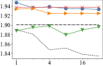
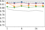
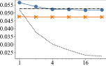
DTR		nDCG@10			EEL		nDCG@10
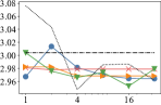
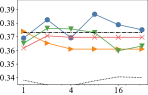
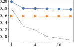
DTR		nDCG@10			EEL		nDCG@10
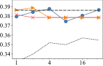
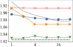
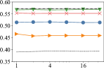
DTR		nDCG@10			EEL		nDCG@10
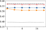
	Sessions		Sessions			Sessions		Sessions

Figure 3. LTR outputs as utility estimates. Performance comparison of PL and PPG search for optimizing different fairness metrics: DTR and EEL (lower is better in both metrics). Top: TREC 2019; middle: TREC 2020; bottom: MSLR. In all cases PPG search achieves comparable results to the baselines (see Appendix B for more details).

5. Results

We run experiments to address the following research questions:

1. Compared to existing methods for ranking fairness optimization, what is the effectiveness of PPG search in finding the fairest ranking for different fairness measures?

2. How does PPG search perform compared to PL for queries with a small number of repeating sessions?

3. Can the possibility of pairwise constraints in PPG search be used to control other measures, e.g., ranking performance, while optimizing fairness?

4. How does an accurate estimate of utility, e.g., the relevance labels, affect different fairness optimization methods?

5.1. Fairness optimization performance

We first address (RQ1) and (RQ2) concerning the performance comparison of PPG search to existing fairness optimization methods. Fig. 3 shows a performance comparison of our PPG search and PL for optimizing DTR and EEL on three datasets TREC 2019, TREC 2020, and MSLR, for different numbers of sessions per query. For both fairness measures, lower means fairer, i.e., better. We omit FOE^H in this figure for better visualization, as it is surpassed by FOE^S in all three tested datasets.

EEL. Regarding (RQ1), we observe in Fig. 3 that for EEL, our PPG method performs better than PL on all three datasets, both being far from the fairness obtained from randomized items. The PL method, after enough sessions, converges to the fairness performance of the LTR output. In terms of ranking performance when optimizing for EEL, PPG is slightly worse than PL on the MSLR and TREC 2019 datasets.

DTR. When optimizing for DTR, PPG and PL both hurt the initial fairness of the LTR output. Here, FOE^S, designed specifically for DTR optimization, has the best performance on all three datasets. On the MSLR and TREC 2020 datasets, PPG and PL perform closely to the randomized items. Comparing PPG and PL to each other, PPG is slightly fairer on the TREC 2019 and MSLR datasets. In the case of DTR optimization for the MSLR dataset, it is interesting to note that randomization slightly hurts fairness of the LTR output, by around $3\%$ relative difference. FOE^S correctly sticks to the LTR output in this case. The message from comparing PPG and PL on the three tested datasets is that, PPG leads to slightly fairer performance than PL when optimized for EEL, while the two perform nearly the same when optimized for DTR.

Small number of sessions. When the number of sessions is limited (RQ2), we see a decisive advantage for PPG compared to PL in EEL. For EEL, on all three datasets, PPG converges at the first session, i.e., it finds a deterministic permutation for one session of each query which has a better fairness value than the expected fairness of PL-generated permutations after $32$ sessions. In this sense, PL can be thought of as the mean$(\cdot)$ aggregator, whereas PPG is the min$(\cdot)$ aggregator; mean$(\cdot)$ needs more sessions to converge to the optimum value. For DTR, PPG needs $4$ sessions to converge, while PL converges after $8$ sessions. Therefore, the answer to (RQ2) on our tested datasets is that before a query is repeated many times, PPG is preferred to PL. The reason is that in PPG the reference permutation is set to the best sampled permutation, so in deterministic scenarios, i.e., with only one session per query, PPG is the go-to method.

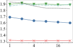
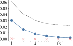
DTR		nDCG@10			EEL		nDCG@10
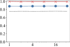
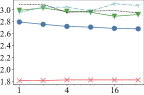
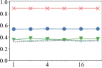
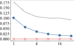
DTR		nDCG@10			EEL		nDCG@10
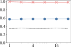
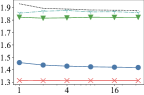
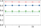
DTR		nDCG@10			EEL		nDCG@10
	Sessions		Sessions			Sessions		Sessions

Figure 4. True relevance labels as utility estimates. Performance comparison of PL and PPG search for optimizing different fairness metrics: DTR and EEL. Top: TREC 2019; middle: TREC 2020; bottom: MSLR (see Appendix B for more details).

5.2. Pairwise constraints

To answer (RQ3) about the effectiveness of pairwise constraints, we set the intra-group fixed-ranking constraint on a PPG model as follows: The items in each fairness group are constrained to have the same ordering as the LTR output. This means that the weight of each edge whose endpoints belong to the same fairness group is initialized by zero and consequently will remain zero during training. This is a conservative way of not hurting the ranking performance too much, while searching for a fair ranking (see Sec. 3.4). The “PPG$~{}+~{}$intra” legend in Fig. 3 shows the results. In this figure we see that in all the cases, the ranking performance, measured by nDCG@10, is noticeably improved by adding the intra-group constraint over PPG. This ranking performance improvement comes with a negligible cost of fairness degradation: in the EEL case, “PPG” and “PPG + intra” have the same fairness performance, while for DTR, there is a slight degradation of less than $3\%$ relative difference in fairness performance on all three datasets. So we can answer (RQ3) positively: using proper pairwise constraints does help to improve other measures, while optimizing for fairness. This possibility is very useful in scenarios where the true relevance labels are unknown and the exact ranking performance cannot be measured. Imposing intra-group fixed-ranking constraints is a conservative way of not hurting our best estimation of the ideal ranking.

5.3. Accurate utility estimates

One advantage of post-processing for fairness optimization is the possibility of improving future fairness for the torso queries. In this section, we investigate the effectiveness of different fairness optimization methods for specialized queries where highly confident, accurate utility estimates are available through tabular models.

Fig. 4 shows the comparison of different fairness optimization methods when accurate relevance labels are known. Here, we only include the results of “PPG + intra”, as we have shown its superiority to the simple “PPG” in Sec. 5.2. For brevity, we only mention “PPG” instead of “PPG + intra” in the following. The gap between the performance of PPG to other baselines is huge, for both fairness and ranking. PPG is the clear winner in all the tested datasets and both fairness metrics. For EEL, PPG is able to achieve the optimal value of $0$. For DTR, PPG comes very close to the optimal value of $1$ on the TREC 2019 and MSLR datasets. Compared with FOE^H and FOE^S, we observe that knowledge of accurate utility estimates helps PL and PPG more and causes them to perform better. This is in contrast with our observation with noisy LTR outputs in Sec. 5.1.

In terms of the ranking performance, we observe that the intra-group fixed-ranking has helped PPG to maintain the ranking near ideal, while minimizing the fairness measure.

6. Conclusion

In this paper, we have defined  probabilistic permutation graph (PPG), a novel representation for permutation distributions. We used PPG as a substitute for PL in black-box optimization of fairness metrics, using the REINFORCE algorithm. Unlike PL which is represented by pointwise logits, PPG is constructed by a reference permutation together with pairwise inversion probabilities. The reference permutation of PPG is very useful in deterministic scenarios.

Our experiments show that PPG search, compared to state-of-the-art post-processing fairness optimization methods, is more robust in finding a deterministic fair permutation for one session, while having comparable performance for expected fairness over larger numbers of sessions. The pairwise inversion probabilities allow us to impose pairwise constraints that can control other objectives while optimizing for fairness. We experimentally verified the effectiveness of such pairwise constraints on controlling the ranking performance. Finally, we have shown that in scenarios such as tabular search, where high quality estimates of utility are available, PPG performs outstandingly well, with a considerable gap to other state-of-the-art fairness optimization methods.

As future work, it would be interesting to test the effectiveness of PPG on other fairness metrics as well as other general permutation optimization problems. Another possible line of work is to apply PPG for an in-processing method as a substitute for PL.

Code and data

To facilitate the reproducibility of our results, this work only made use of publicly available data and our experimental implementation is publicly available at https://github.com/AliVard/PPG.

Appendix A Log Derivative of Probability Distribution

Here we discuss the approximate log derivative of the probability distribution, given in Eq. (9). Rewriting Eq. (8) we have:

$$\frac{\partial\log P(E_{\pi})}{\partial w_{e}}=\underbrace{\frac{\mathbb{I}\bigl{(}e\in E_{\pi}\bigr{)}-w_{e}}{w_{e}\cdot\bigl{(}1-w_{e}\bigr{)}}}_{\alpha_{w}}-\underbrace{\frac{1}{\rho}\frac{\partial\rho}{\partial w_{e}}}_{\beta_{\rho,w}}.$$

The first term, $\alpha_{w}$, only depends on the weight $w_{e}$ and sampled graph $E_{\pi}$. However, the second term, $\beta_{\rho,w}$, depends on $\rho$ which cannot be calculated feasibly because of the exponential size of the permutation space. Consequently, we explain why it is save to consider $\alpha_{w}-\beta_{\rho,w}\approx\alpha_{w}$ in gradient descent. First note that, fixing all the weights other than $w_{e}$, $\rho$ is a linear function of $w_{e}$:

$$\rho=w_{e}\cdot A+\bigl{(}1-w_{e}\bigr{)}\cdot B,$$

where $A$ is the probability sum of all the permutation graphs containing $e$ and $B$ is the probability sum of all the permutation graphs not containing $e$. Therefore, we have

$$\beta_{\rho,w}=\frac{A-B}{w_{e}\cdot\bigl{(}A-B\bigr{)}+B}.$$

We know from graph theory that (Dushnik and Miller, 1941):

(12) $$E\in\mathcal{P}\Rightarrow\bar{E}\in\mathcal{P},$$

where $\bar{E}$ is the complement graph of $E$. For training the PPG weights, we initialize all the weights to $0.5$ and slightly change them using the gradients. Simple counting shows that, when all the edges have a $0.5$ probability of sampling, we have:

(13) $$A=B=\frac{n!}{2^{\frac{n(n-1)}{2}}},$$

which means that for the initial weights $\beta_{\rho,w}=0$. We further show that, even when $\beta_{\rho,w}\neq 0$, the gradient and $\alpha_{w}$ always have the same sign. This is a critical condition in gradient descent with small learning rate, as the weights are guaranteed to update in the correct direction. To show $\alpha_{w}$ and $\alpha_{w}-\beta_{\rho,w}$ always have the same sign, we notice that when $\alpha_{w}$ and $\beta_{\rho,w}$ have different signs, the proposition is true. It remains to prove the proposition for the case where $\alpha_{w}$ and $\beta_{\rho,w}$ have the same signs:

1. Case 1: $\alpha_{w}=\frac{1}{w_{e}}>0$ and $\beta_{\rho,w}>0$

   (14) $$w_{e}(A-B)+B>A-B\xRightarrow{(A-B>0)}\beta_{\rho,w}<\frac{1}{w_{e}}.$$

2. Case 2: $\alpha_{w}=\frac{-1}{1-w_{e}}<0$ and $\beta_{\rho,w}<0$

   (15) $$\begin{split}&A\cdot w_{e}+B(1-w_{e})>-(A-B)(1-w_{e})>0\\ &\xRightarrow{(A-B<0)}-\beta_{\rho,w}<\frac{1}{1-w_{e}}.\end{split}$$

To sum up, we have shown that in the working range of weights, i.e. $\approx 0.5$, we have $\beta_{\rho,w}\approx 0$. And more importantly, in general, $\alpha_{w}$ and $\alpha_{w}-\beta_{\rho,w}$ always have the same sign, ensuring that the gradient descent updates the weights in the correct direction. Our experiments show a very negligible sensitivity of PPG search to the learning rate, which translates to negligible sensitivity to the gradient size.

Appendix B Results for Small Number of Sessions

Table 1. Results on 4 sessions with LTR generated labels.

			Fairness		NDCG@10
		Model	DTR $\downarrow$	EEL $\downarrow$	DTR $\uparrow$	EEL $\uparrow$
TREC 2019		$FOE^{S}$	1.898	-	0.805	-
		$FOE^{H}$	1.944	-	0.803	-
		PL	1.939	0.052	0.817	0.793
		PPG	1.925	0.047	0.806	0.780
		PPG + intra	1.938	0.047	0.812	0.790
		LTR output	1.901	0.053	0.816	0.798
		RAND	1.848	0.030	0.792	0.754
TREC 2020		$FOE^{S}$	2.966	-	0.376	-
		$FOE^{H}$	3.047	-	0.371	-
		PL	2.981	0.180	0.369	0.388
		PPG	2.969	0.158	0.361	0.378
		PPG + intra	2.979	0.158	0.370	0.379
		LTR output	3.004	0.173	0.373	0.386
		RAND	2.948	0.118	0.334	0.352
MSLR-qs		$FOE^{S}$	1.835	-	0.567	-
		$FOE^{H}$	1.842	-	0.526	-
		PL	1.885	0.123	0.517	0.535
		PPG	1.868	0.108	0.459	0.510
		PPG + intra	1.913	0.108	0.552	0.564
		LTR output	1.824	0.114	0.572	0.572
		RAND	1.893	0.081	0.395	0.392

Table 1 and 2 contain the results of all models on 4 sessions with LTR outputs as utility estimates and knowledge of the true relevance labels, respectively. In the case of a limited number of sessions and LTR outputs as utility estimates (Table 1), PPG has a slight advantage compared to PL when optimizing for both EEL and DTR in all three tested datasets. In this case, FOE^S, specifically designed for DTR optimization, leads to the fairest ranking in all three datasets. When the true relevance labels are known (Table 2), PPG search outperforms the baselines by a noticeable margin (20%, 33%, and 8% relative decrease for DTR and 100%, 100%, and 30% relative decrease for EEL, compared to the runner up, in TREC 2019, TREC 2020, and MSLR, respectively), obtaining the fairest ranking policies while achieving NDCG scores close to the ideal ranking. Note that the scores reported in Table 1 and 2 are from two separate experiments which explains the small differences in the results for the RAND baseline.

Table 2. Results on 4 sessions with true relevance labels.

			Fairness		NDCG@10
		Model	DTR $\downarrow$	EEL $\downarrow$	DTR $\uparrow$	EEL $\uparrow$
TREC 2019		$FOE^{S}$	1.898	-	0.799	-
		$FOE^{H}$	1.885	-	0.799	-
		PL	1.632	0.008	0.892	0.881
		PPG	1.320	0.000	0.881	0.900
		PPG + intra	1.309	0.000	0.978	0.989
		Ideal ranking	1.668	0.014	1.000	1.000
		RAND	1.870	0.031	0.794	0.754
TREC 2020		$FOE^{S}$	2.974	-	0.368	-
		$FOE^{H}$	3.044	-	0.357	-
		PL	2.722	0.036	0.545	0.577
		PPG	2.141	0.000	0.574	0.819
		PPG + intra	1.825	0.000	0.894	0.984
		Ideal ranking	2.538	0.023	1.000	1.000
		RAND	2.957	0.107	0.337	0.349
MSLR-qs		$FOE^{S}$	1.818	-	0.564	-
		$FOE^{H}$	1.877	-	0.504	-
		PL	1.429	0.030	0.810	0.873
		PPG	1.395	0.021	0.619	0.821
		PPG + intra	1.313	0.021	0.950	0.979
		Ideal ranking	1.548	0.027	1.000	1.000
		RAND	1.889	0.081	0.394	0.392

References

- (1)
- Asudeh et al. (2019) Abolfazl Asudeh, HV Jagadish, Julia Stoyanovich, and Gautam Das. 2019. Designing Fair Ranking Schemes. In SIGMOD. 1259–1276.
- Baeza-Yates (2018) Ricardo Baeza-Yates. 2018. Bias on the Web. Commun. ACM 61, 6 (2018), 54–61.
- Bello et al. (2016) Irwan Bello, Hieu Pham, Quoc V Le, Mohammad Norouzi, and Samy Bengio. 2016. Neural Combinatorial Optimization with Reinforcement Learning. arXiv preprint arXiv:1611.09940 (2016).
- Berny (2000) Arnaud Berny. 2000. Selection and Reinforcement Learning for Combinatorial Optimization. In International Conference on Parallel Problem Solving from Nature. Springer, 601–610.
- Biega et al. (2019) Asia J. Biega, Fernando Diaz, Michael D. Ekstrand, and Sebastian Kohlmeier. 2019. Overview of the TREC 2019 Fair Ranking Track. In The Twenty-Eighth Text REtrieval Conference (TREC 2019) Proceedings.
- Biega et al. (2018) Asia J Biega, Krishna P Gummadi, and Gerhard Weikum. 2018. Equity of Attention: Amortizing Individual Fairness in Rankings. In SIGIR. 405–414.
- Birkhoff (1940) Garrett Birkhoff. 1940. Lattice Theory. AMS.
- Celis et al. (2020) L Elisa Celis, Anay Mehrotra, and Nisheeth K Vishnoi. 2020. Interventions for Ranking in the Presence of Implicit Bias. In FAT*. 369–380.
- Celis et al. (2018) L Elisa Celis, Damian Straszak, and Nisheeth K Vishnoi. 2018. Ranking with Fairness Constraints. In ICALP. 28:1–28:15.
- Diaz et al. (2020) Fernando Diaz, Bhaskar Mitra, Michael D Ekstrand, Asia J Biega, and Ben Carterette. 2020. Evaluating Stochastic Rankings with Expected Exposure. In Proceedings of the 29th ACM International Conference on Information & Knowledge Management. 275–284.
- Dushnik and Miller (1941) Ben Dushnik and Edwin W Miller. 1941. Partially Ordered Sets. American Journal of Mathematics 63, 3 (1941), 600–610.
- Fligner and Verducci (1988) Michael A. Fligner and Joseph S. Verducci. 1988. Multistage Ranking Models. J. Amer. Statist. Assoc. 83, 403 (1988), 892–901. http://www.jstor.org/stable/2289322
- Gadetsky et al. (2020) Artyom Gadetsky, Kirill Struminsky, Christopher Robinson, Novi Quadrianto, and Dmitry Vetrov. 2020. Low-variance Black-box Gradient Estimates for the Plackett-Luce Distribution. In Proceedings of the AAAI Conference on Artificial Intelligence, Vol. 34. 10126–10135.
- Geyik et al. (2019) Sahin Cem Geyik, Stuart Ambler, and Krishnaram Kenthapadi. 2019. Fairness-aware Ranking in Search & Recommendation Systems with Application to Linkedin Talent Search. In SIGKDD. 2221–2231.
- Grainger (2021) Trey Grainger. 2021. AI Powered Search. Manning Publications.
- Gumbel (1954) Emil Julius Gumbel. 1954. Statistical Theory of Extreme Values and Some Practical Applications: A Series of Lectures. Vol. 33. US Government Printing Office.
- Heuss et al. (2022) Maria Heuss, Fatemeh Sarvi, and Maarten de Rijke. 2022. Fairness of Exposure in Light of Incomplete Exposure Estimation. In SIGIR 2022: 45th international ACM SIGIR Conference on Research and Development in Information Retrieval. ACM.
- Joachims et al. (2017) Thorsten Joachims, Adith Swaminathan, and Tobias Schnabel. 2017. Unbiased Learning-to-Rank with Biased Feedback. In Proceedings of the Tenth ACM International Conference on Web Search and Data Mining. ACM, 781–789.
- Katariya et al. (2016) Sumeet Katariya, Branislav Kveton, Csaba Szepesvari, and Zheng Wen. 2016. DCM Bandits: Learning to Rank with Multiple Clicks. In Proceedings of The 33rd International Conference on Machine Learning (Proceedings of Machine Learning Research), Maria Florina Balcan and Kilian Q. Weinberger (Eds.), Vol. 48. PMLR, New York, New York, USA, 1215–1224. https://proceedings.mlr.press/v48/katariya16.html
- Kırnap et al. (2021) Ömer Kırnap, Fernando Diaz, Asia Biega, Michael Ekstrand, Ben Carterette, and Emine Yilmaz. 2021. Estimation of Fair Ranking Metrics with Incomplete Judgments. In Proceedings of the Web Conference 2021. 1065–1075.
- Kleinberg et al. (2017) Jon Kleinberg, Sendhil Mullainathan, and Manish Raghavan. 2017. Inherent Trade-Offs in the Fair Determination of Risk Scores. In 8th Innovations in Theoretical Computer Science Conference (ITCS 2017) (2017) (Leibniz International Proceedings in Informatics (LIPIcs)), Christos H. Papadimitriou (Ed.), Vol. 67. Schloss Dagstuhl–Leibniz-Zentrum fuer Informatik, 43:1–43:23. https://doi.org/10.4230/LIPIcs.ITCS.2017.43
- Lagrée et al. (2016) Paul Lagrée, Claire Vernade, and Olivier Cappe. 2016. Multiple-Play Bandits in the Position-Based Model. In Advances in Neural Information Processing Systems, Vol. 29. Curran Associates, Inc.
- Li et al. (2020) Chang Li, Branislav Kveton, Tor Lattimore, Ilya Markov, Maarten de Rijke, Csaba Szepesvári, and Masrour Zoghi. 2020. BubbleRank: Safe Online Learning to Re-Rank via Implicit Click Feedback. In Proceedings of The 35th Uncertainty in Artificial Intelligence Conference (Proceedings of Machine Learning Research), Vol. 115. PMLR, 196–206.
- Luce (1959) R Duncan Luce. 1959. Individual Choice Behavior. John Wiley.
- Maddison et al. (2014) Chris J Maddison, Daniel Tarlow, and Tom Minka. 2014. A* Sampling. In Advances in Neural Information Processing Systems, Z. Ghahramani, M. Welling, C. Cortes, N. Lawrence, and K. Q. Weinberger (Eds.), Vol. 27. Curran Associates, Inc.
- Mavridis et al. (2020) Themistoklis Mavridis, Soraya Hausl, André Mende, and Roberto Pagano. 2020. Beyond Algorithms: Ranking at Scale at Booking.com. In ComplexRec-ImpactRS@RecSys.
- McConnell and Spinrad (1999) Ross M. McConnell and Jeremy P. Spinrad. 1999. Modular decomposition and transitive orientation. Discrete Mathematics 201, 1 (1999), 189–241. https://doi.org/10.1016/S0012-365X(98)00319-7
- Mehrotra et al. (2018) Rishabh Mehrotra, James McInerney, Hugues Bouchard, Mounia Lalmas, and Fernando Diaz. 2018. Towards a Fair Marketplace: Counterfactual Evaluation of the Trade-off between Relevance, Fairness & Satisfaction in Recommendation Systems. In CIKM. 2243–2251.
- Morik et al. (2020) Marco Morik, Ashudeep Singh, Jessica Hong, and Thorsten Joachims. 2020. Controlling Fairness and Bias in Dynamic Learning-to-rank. In SIGIR. 429–438.
- Oosterhuis (2021) Harrie Oosterhuis. 2021. Computationally Efficient Optimization of Plackett-Luce Ranking Models for Relevance and Fairness. In Proceedings of the 44th International ACM SIGIR Conference on Research and Development in Information Retrieval. Association for Computing Machinery, New York, NY, USA, 1023–1032. https://doi.org/10.1145/3404835.3462830
- Oosterhuis and de Rijke (2021) Harrie Oosterhuis and Maarten de de Rijke. 2021. Robust Generalization and Safe Query-Specializationin Counterfactual Learning to Rank. In Proceedings of the Web Conference 2021. 158–170.
- Plackett (1975) Robin L Plackett. 1975. The Analysis of Permutations. Journal of the Royal Statistical Society: Series C (Applied Statistics) 24, 2 (1975), 193–202.
- Qin and Liu (2013) Tao Qin and Tie-Yan Liu. 2013. Introducing LETOR 4.0 datasets. arXiv preprint arXiv:1306.2597 (2013).
- Raj et al. (2020) Amifa Raj, Connor Wood, Ananda Montoly, and Michael D Ekstrand. 2020. Comparing Fair Ranking Metrics. arXiv preprint arXiv:2009.01311 (2020).
- Sapiezynski et al. (2019) Piotr Sapiezynski, Wesley Zeng, Ronald E Robertson, Alan Mislove, and Christo Wilson. 2019. Quantifying the Impact of User Attentionon Fair Group Representation in Ranked Lists. In WWW. 553–562.
- Sarvi et al. (2021) Fatemeh Sarvi, Maria Heuss, Mohammad Aliannejadi, Sebastian Schelter, and Maarten de Rijke. 2021. Understanding and Mitigating the Effect of Outliers in Fair Ranking. arXiv preprint arXiv:2112.11251 (2021).
- Singh and Joachims (2018) Ashudeep Singh and Thorsten Joachims. 2018. Fairness of Exposure in Rankings. In Proceedings of the 24th ACM SIGKDD International Conference on Knowledge Discovery & Data Mining (KDD ’18). Association for Computing Machinery, New York, NY, USA, 2219–2228. https://doi.org/10.1145/3219819.3220088
- Singh and Joachims (2019) Ashudeep Singh and Thorsten Joachims. 2019. Policy Learning for Fairness in Ranking. arXiv preprint arXiv:1902.04056 (2019).
- Sorokina and Cantu-Paz (2016) Daria Sorokina and Erick Cantu-Paz. 2016. Amazon Search: The Joy of Ranking Products. In Proceedings of the 39th International ACM SIGIR Conference on Research and Development in Information Retrieval (SIGIR ’16). Association for Computing Machinery, New York, NY, USA, 459–460. https://doi.org/10.1145/2911451.2926725
- Stoyanovich et al. (2018) Julia Stoyanovich, Ke Yang, and HV Jagadish. 2018. Online Set Selection with Fairness and Diversity Constraints. In EDBT. 241–252.
- Trotman et al. (2017) Andrew Trotman, Jon Degenhardt, and Surya Kallumadi. 2017. The architecture of ebay search. In eCOM@ SIGIR.
- Vardasbi et al. (2021) Ali Vardasbi, Maarten de Rijke, and Ilya Markov. 2021. Mixture-Based Correction for Position and Trust Bias in Counterfactual Learning to Rank. In Proceedings of the 30th ACM International Conference on Information & Knowledge Management. 1869–1878.
- Vardasbi et al. (2020) Ali Vardasbi, Harrie Oosterhuis, and Maarten de Rijke. 2020. When Inverse Propensity Scoring does not Work: Affine Corrections for Unbiased Learning to Rank. In Proceedings of the 29th ACM International Conference on Information & Knowledge Management. ACM, 1475–1484.
- Verma and Rubin (2018) Sahil Verma and Julia Rubin. 2018. Fairness Definitions Explained. In 2018 IEEE/ACM International Workshop on Software Fairness (FairWare). 1–7. https://doi.org/10.23919/FAIRWARE.2018.8452913
- Williams (1992) Ronald J Williams. 1992. Simple Statistical Gradient-following Algorithms for Connectionist Reinforcement Learning. Machine learning 8, 3 (1992), 229–256.
- Yadav et al. (2019) Himank Yadav, Zhengxiao Du, and Thorsten Joachims. 2019. Policy-Gradient Training of Fair and Unbiased Ranking Functions. arXiv preprint arXiv:1911.08054 (2019).
- Yadav et al. (2021) Himank Yadav, Zhengxiao Du, and Thorsten Joachims. 2021. Policy-Gradient Training of Fair and Unbiased Ranking Functions. In Proceedings of the 44th International ACM SIGIR Conference on Research and Development in Information Retrieval. Association for Computing Machinery, New York, NY, USA, 1044–1053. https://doi.org/10.1145/3404835.3462953
- Yang and Stoyanovich (2017) Ke Yang and Julia Stoyanovich. 2017. Measuring Fairness in Ranked Outputs. In SSDBM. 1–6.
- Zehlike et al. (2017) Meike Zehlike, Francesco Bonchi, Carlos Castillo, Sara Hajian, Mohamed Megahed, and Ricardo Baeza-Yates. 2017. FA*IR: A Fair Top-k Ranking Algorithm. In CIKM. 1569–1578.
- Zehlike et al. (2021) Meike Zehlike, Ke Yang, and Julia Stoyanovich. 2021. Fairness in Ranking: A Survey. arXiv preprint arXiv:2103.14000 (2021).
- Zoghi et al. (2016) Masrour Zoghi, Tomáš Tunys, Lihong Li, Damien Jose, Junyan Chen, Chun Ming Chin, and Maarten de Rijke. 2016. Click-based Hot Fixes for Underperforming Torso Queries. In Proceedings of the 39th Annual International ACM SIGIR Conference on Research and Development in Information Retrieval (SIGIR). ACM.