First concurrent extraction of the leading-order scalar and spin proton polarizabilities

Abstract

We performed the first simultaneous extraction of the six leading-order proton polarizabilities. We reached this milestone thanks to both new high-quality experimental data and an innovative bootstrap-base fitting method. These new results provide a self-consistent and fundamental benchmark for all future theoretical and experimental polarizability estimates.

I Introduction

Understanding the hadron structure in the non-perturbative regime of quantum chromodynamics (QCD) is one of the major challenge of modern physics. We can classify hadrons in terms of their global properties, such as mass and spin, but we can not fully explain how these properties emerge from the underlying dynamics of the hadron’s interior. A clean probe to investigate the internal structure of hadrons is the Compton scattering process that gives access to observables with a clear interpretation in terms of structure-dependent properties of the hadrons. In particular, real Compton scattering (RCS) at low energies is parametrized by polarizabilities that describe the response of the charge and magnetization distributions inside the nucleon to an applied quasi-static electromagnetic field. These structure constants are fundamental properties of the nucleon and their determination has driven a relevant experimental effort in the last few years Martel et al. (2015); Sokhoyan et al. (2017); Paudyal et al. (2020); Mornacchi et al. (2022); Li et al. (2022).

The effective multipole interactions for the coupling of the electric ($\vec{E}$) and magnetic ($\vec{H}$) fields of the photon with the internal structure of the nucleon is described at leading order in terms of the electric ($\alpha_{E1}$) and magnetic ($\beta_{M1}$) scalar polarizabilities Babusci et al. (1998); Holstein et al. (2000):

$$H^{(2)}_{eff}=-4\pi\Bigl{[}\frac{1}{2}\alpha_{E1}\vec{E}^{2}+\frac{1}{2}\beta_{M1}\vec{H}^{2}\Bigr{]},$$ (1)

while the four spin polarizabilities ($\gamma_{\dots}$) show up in the subleading terms:

$$H^{(3)}_{eff} =-4\pi\Bigl{[}\frac{1}{2}\gamma_{E1E1}\vec{\sigma}\cdot(\vec{E}\times\dot{\vec{E}})+\frac{1}{2}\gamma_{M1M1}\vec{\sigma}\cdot(\vec{H}\times\dot{\vec{H}})$$

$$\quad-\gamma_{M1E2}E_{ij}\sigma_{i}H_{j}+\gamma_{E1M2}H_{ij}\sigma_{i}E_{j}\Bigr{]},$$ (2)

where $\vec{\sigma}$ are the proton’s Pauli spin matrices, $\dot{\vec{E}}=\partial_{t}\vec{E}$ and $E_{ij}=\frac{1}{2}(\nabla_{i}E_{j}+\nabla_{j}E_{i}$) are partial derivatives with respect to time and space, respectively.

In addition to being fundamental properties of the nucleon, polarizabilities play a profound role in precision atomic physics, in the evaluation of the nuclear corrections to atomic energy levels Drell and Sullivan (1967); Bernabeu and Ericson (1983); Faustov and Martynenko (2000); Martynenko (2006); Carlson and Vanderhaeghen (2011) and in astrophysics, influencing neutron star properties Bernabeu et al. (1974).

Despite their evident importance in a broad range of physics topics, up to now a self-consistent experimental extraction of all the different polarizability values has not been possible, due to the scarce quality of the available database (see, for instance, Ref. Pasquini et al. (2019)). In all existing fits of the RCS data, some of the polarizabilities have been fixed either using theoretical calculations Griesshammer et al. (2012); McGovern et al. (2013); Lensky and McGovern (2014); Griesshammer et al. (2016) or empirical evaluations from other reactions Krupina et al. (2018), or, at most, have been constrained to vary within certain intervals Pasquini et al. (2019). The situation has recently improved with the first measurements of the double-polarization observables $\Sigma_{2x}$ Martel et al. (2015) and $\Sigma_{2z}$ Paudyal et al. (2020) and new data for the unpolarized differential cross sections and the single-polarized $\Sigma_{3}$ asymmetry Sokhoyan et al. (2017); Mornacchi et al. (2022); Li et al. (2022). The beam asymmetry is defined as (Babusci et al., 1998):

$$\Sigma_{3}=\dfrac{d\sigma_{\parallel}-d\sigma_{\perp}}{d\sigma_{\parallel}+d\sigma_{\perp}},$$ (3)

where $d\sigma_{\parallel(\perp)}$ is the polarized cross section obtained with a photon beam polarized parallel (or perpendicularly) to the scattering plane and an unpolarized target. In a similar way, the double-polarization asymmetries can be defined as:

$$\Sigma_{2x}=\dfrac{d\sigma^{R}_{+x}-d\sigma^{L}_{\pm x}}{d\sigma^{R}_{+x}+d\sigma^{L}_{\pm x}},~{}~{}\text{and}~{}~{}\Sigma_{2z}=\dfrac{d\sigma^{R}_{+z}-d\sigma^{L}_{\pm z}}{d\sigma^{R}_{+z}+d\sigma^{L}_{\pm z}},$$ (4)

where $d\sigma^{R(L)}_{\pm x}$ is the polarized cross section obtained with circular right-handed (left-handed) photon polarization and target spin aligned transversely $(\pm x)$ with respect to the incident beam direction, while $d\sigma^{R(L)}_{\pm z}$ is obtained with the target spin aligned longitudinally $(\pm z)$ with respect to the incident beam direction.

In particular, the work from Mornacchi et al. Mornacchi et al. (2022) provides the highest statistics proton RCS single dataset ever obtained below the pion photoproduction threshold, with 60 unpolarized differential cross section points and 36 beam asymmetry points measured over a large angular range and with small statistical and systematic errors. Therefore, it represents a significant improvement for a more accurate extractions of all the different polarizability values.

In this paper we present the first consistent and simultaneous fit of the six leading-order static proton polarizabilities. It has been obtained thanks to both the new experimental data and an innovative bootstrap-base fitting method Pedroni and Sconfietti (2020). This algorithm has already been deployed successfully for the extraction of the proton scalar dynamical and static polarizabilities from low-energy RCS data Pasquini et al. (2018, 2019). The theoretical framework used for this extraction is based on fixed-$t$ subtracted dispersion relations (DRs) Drechsel et al. (1999); Holstein et al. (2000); Pasquini et al. (2007). The theoretical uncertainties associated to the model dependence of our results are also evaluated by using, as input, pion photoproduction amplitudes obtained from three different partial wave analyses (PWAs) of the available experimental data: BnGa-2019 Anisovich et al. (2016), MAID-2021 Drechsel et al. (2007); Kashevarov and Tiator (2021), and SAID-MA19 Briscoe et al. (2019). This is the very first time that such a comprehensive and self-consistent study on the simultaneous extraction of all the six leading-order proton polarizabilities from RCS data is performed.

II Database selection and fit procedure

The proton RCS database used for this work consists of two main sets: the unpolarized differential cross section data, and the (single and double) polarization asymmetries. The former can be further divided into low- and high-energy data, namely data for which the incoming photon energy $E_{\gamma}$ is below or above the pion photoproduction threshold ($\sim 150$ MeV), respectively.

For the low-energy set, in addition to the new data from Refs. Mornacchi et al. (2022); Li et al. (2022), we used the same selection extensively discussed in a previous work by Pasquini et al. Pasquini et al. (2019), which includes datasets from Refs. Oxley (1958); Hyman et al. (1959); Goldansky et al. (1960); Bernardini et al. (1960); Pugh et al. (1957); Baranov et al. (1974, 1975); Federspiel et al. (1991); Zieger et al. (1992); Hallin et al. (1993); MacGibbon et al. (1995); de León et al. (2001). For the high-energy set, thanks to the DR model used for the theoretical framework, we were able to consider data measured up to $E_{\gamma}=300$ MeV (corresponding to the $2\pi$ photoproduction threshold), thus extending the range used in the fits of Refs. McGovern et al. (2013); Pasquini et al. (2019). Furthermore, only for these high-energy data, we decided to narrow the selection to the new-generation experiments, namely the measurements performed using tagged photon facilities (see, for instance, the review of Ref. Schumacher (2005)). Their main advantage, in addition to a more reliable photon flux determination, is that the incoming photon energy is known with a resolution of a few MeV. This is an essential ingredient to reject the overwhelming background coming from the single $\pi^{0}$ photoproduction channel that has a cross section by two orders of magnitude higher than Compton scattering process, and can mimic the Compton signature when one of the two photons coming from the $\pi^{0}$ decay escapes the particle detection. The available datasets for the unpolarized cross section come from two different facilities: MAMI Peise and Schumacher (1996); Molinari et al. (1996); Wissmann et al. (1999); Wolf et al. (2001); Galler et al. (2001); Camen et al. (2002) (with also few data above threshold from Ref. de León et al. (2001)) and LEGS Tonnison et al. (1998); Blanpied et al. (2001).

The polarization observables have enhanced sensitivity to the spin polarizabilities Pasquini et al. (2007); Griesshammer et al. (2018), hence are crucial for the extraction of these structure constants. The adopted datasets include three different polarization observables: $\Sigma_{2x}$ Martel et al. (2015), $\Sigma_{2z}$ Paudyal et al. (2020), and $\Sigma_{3}$ both below Sokhoyan et al. (2017); Mornacchi et al. (2022); Li et al. (2022) and above Blanpied et al. (2001) pion photoproduction threshold.

The fit to extract the leading-order scalar and spin polarizabilities was performed using a bootstrap-based method Pedroni and Sconfietti (2020) that consists of randomly generating $N$ Monte Carlo replicas of the fitted experimental database, where each data point $e_{i,j}^{(0)}$ is replaced by:

$$e_{i,j}^{(0)}\rightarrow e_{i,j}^{(b)}=(1+\delta_{j,b})(e_{i,j}^{(0)}+r_{i,j,b}\sigma^{(0)}_{i,j}).$$ (5)

The indices $i$, $j$, and $b$ run over the number of data points in each dataset, the number of datasets, and the bootstrap replica, respectively; $r_{i,j,b}$ is a random number extracted from the normal distribution $\mathcal{N}(0,1)$, and $\delta_{j,b}$ is a random variable that accounts for the effect of the common systematic errors, independently for each dataset. From each of these simulated databases, a set of fitted parameters is extracted. The mean and standard deviation of the obtained distributions give then the best value and the error for each of the fitted parameters. This technique offers several advantages compared to other fitting procedures, especially when different datasets are used together, as in the present work: i) a straightforward inclusion of common systematic uncertainties without any a priori assumption on their distributions and without introducing any additional fit parameter; ii) the probability distribution of the fit parameters (often non-gaussian) is obtained directly by the procedure itself; iii) the uncertainties on possible nuisance model parameters are easily and directly taken into account in the sampling procedure; iv) the correct fit $p$-value is always provided when systematic uncertainties are present and in all the other cases when the goodness-of-fit distribution is not given by the $\chi^{2}$-distribution.

In the first step of our analysis, we checked the consistency of the selected database by looking at the distribution of the normalized residual for each of the largest datasets (e.g., with more than 40 data points): the unpolarized cross section from the A2 Mornacchi et al. (2022), the TAPS de León et al. (2001), and the LARA Wolf et al. (2001) Collaborations; and the unpolarised cross section and beam asymmetry from the LEGS Blanpied et al. (2001) Collaboration.

Since the cross section data from LARA and LEGS are known to be in significant disagreement between each other (see, for instance, Ref. Griesshammer et al. (2012)), we performed a preliminary test by alternatively including LARA or LEGS data in the fit database and simultaneously fitting all six polarizabilities using the MAID-2021 Drechsel et al. (2007); Kashevarov and Tiator (2021) multipole solution.

For each of the two configurations, we took the output polarizability best-values, calculated the residual distribution for each dataset, and produced a probability plot Chambers et al. (1983) for assessing the residual normal distribution. In all cases, the residuals were found to follow fairly well the expected normal distribution for all the selected datasets (see Fig.1 of the Supplemental Material sup , where the probability plots refer to the test without the LEGS data), except for the unpolarized cross section from both the LEGS and LARA Collaborations, as shown in Fig. 1. We repeated the same test using the SAID-MA19 Briscoe et al. (2019) and BnGa-2019 Anisovich et al. (2016) PWAs and obtained very similar results. Given also the small fit $p$-values, i.e., $\simeq 5\cdot 10^{-4}$ and $\simeq 1\cdot 10^{-2}$ for the LEGS and LARA data, respectively, with all the PWA inputs, we excluded both sets from the database of the present work.

Although the data for the photon asymmetry $\Sigma_{3}$ above threshold are from the same dataset of the LEGS unpolarized cross section, they give a consistent residual plot (see Fig. 1 of the Supplemental Material sup ). Such an agreement is not surprising since, as noted, e.g., in Ref. Griesshammer et al. (2012), most of the possible systematic biases cancel out in an asymmetry observable.

Taking all these considerations together, 25 datasets for a total of 388 points were included in the fit. The angular and energy coverage of all the used datasets are listed in the Supplemental Material sup .

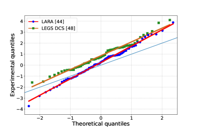
Figure 1: Probability plots using the normalized residuals for the unpolarized cross section from the LARA Wolf et al. (2001) and the LEGS Blanpied et al. (2001) Collaborations, obtained from a global fit using the MAID-2021 multipole solution Drechsel et al. (2007); Kashevarov and Tiator (2021). The points are expected to lie on the bisector (in cyan) if their residuals are normally distributed. The red and orange lines show a linear regression fit to the points from the LARA and LEGS data, respectively, to help the comparison with the expected distribution.

III Results and Discussion

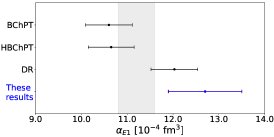
(a) $\alpha_{E1}$

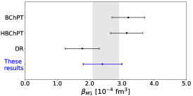
(b) $\beta_{M1}$

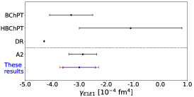
(c) $\gamma_{E1E1}$

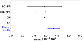
(d) $\gamma_{M1M1}$

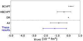
(e) $\gamma_{E1M2}$

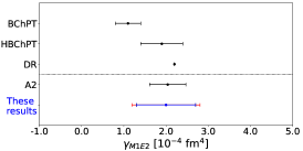
(f) $\gamma_{M1E2}$

Figure 2: Values of the leading-order static proton polarizabilities obtained from the fit procedure. In each panel, our new results are reported in blue. The blue error bars represent the fit error only, the increase in the total error due to the inclusion of the systematic contribution from the model dependency is shown in red. For the two scalar polarizabilities in panels a) and b), DR Pasquini et al. (2019), HBChPT McGovern et al. (2013), and BChPT Lensky and McGovern (2014) refer to three extractions within DR Drechsel et al. (1999); Holstein et al. (2000); Pasquini et al. (2007), HBChPT Griesshammer et al. (2016, 2016), and BChPT Lensky and Pascalutsa (2010) frameworks, respectively. In all cases, most of the spin polarizabilities were fixed to a given value. For the four spin polarizabilities in panels c) to f), some of the existing extractions and theoretical predictions are shown below and above the dotted line, respectively. In particular, A2 refers to the most recent experimental extraction Paudyal et al. (2020), where both scalar polarizabilities were fixed to the PDG values Zyla et al. (2020). DR Holstein et al. (2000), HBChPT McGovern et al. (2013); Griesshammer et al. (2016), and BChPT Lensky et al. (2015) above the dotted line refer to theoretical predictions using different approaches.

A total of $N=10^{4}$ bootstrapped samples of the database was generated and the minimization was performed at the end of each iteration with all six proton polarizabilities treated as free parameters. For convenience, we used as actual fit parameters some linear combinations of the scalar and spin polarizabilities: $\alpha_{E1}\pm\beta_{M1}$, $\gamma_{E1E1}$, $\gamma_{M1M1}$, $\gamma_{0}=-\gamma_{E1E1}-\gamma_{M1M1}-\gamma_{E1M2}-\gamma_{M1E2}$, and $\gamma_{\pi}=-\gamma_{E1E1}+\gamma_{M1M1}-\gamma_{E1M2}+\gamma_{M1E2}$. The last term, $\gamma_{\pi}$, is the sum of the dispersive contribution $\gamma_{\pi}^{{\rm disp}}$, to be fitted to the data, and the pion-pole contribution, fixed to $\gamma_{\pi}^{{\rm\pi^{0}-pole}}=-46.7$ Schumacher (2005). The choice of the fit parameters allows for a direct comparison, as a consistency check, of the fit results for $\alpha_{E1}+\beta_{M1}$ and $\gamma_{0}$ to the available experimental predictions of the Baldin de León et al. (2001); Gryniuk et al. (2015); Hagelstein et al. (2016); Strakovsky et al. (2022) and Gellmann-Goldberger-Thirring (GGT) Pasquini et al. (2010); Gryniuk et al. (2015); Hagelstein et al. (2016); Strakovsky et al. (2022) sum rule values, respectively, obtained using data for the total photoabsorption cross section. When present, point-to-point systematic errors were added in quadrature to the statistical errors, while common systematic scale factors were treated as in the previous bootstrap extractions by Pasquini et al. Pasquini et al. (2018, 2019), namely they are assumed to follow a uniform distribution, unless otherwise specified in the original publication. Moreover, when multiple systematic sources are given, the final error is the product of all the generated random uniform variables.

We performed the minimizations by using the nonlinear least-squares fitting routines of the GSL library Galassi et al. (2009). As a consistency check of this procedure, both the gradient and the simplex methods were used as best-fit algorithms and identical results were obtained. The entire procedure was performed for the three PWAs. The obtained distributions for each parameter are reported in the Supplemental Material sup . The parameter distributions obtained using the three different PWA inputs have the same shape and differ only for a shift in their central values. For this reason, we evaluated the central polarizability values as the mathematical average of the three different sets of fit values. Additionally, the largest of the differences between each set of fit values and the average was used to estimate an additional model error (conservatively considered as a standard deviation) due to dependence on the PWA used as input in the DRs. The resulting best-fit values are:

$${}\alpha_{E1}+\beta_{M1}=\left(15.1\pm 0.7\,\hbox{(fit)}\pm 0.1\,\hbox{(model)}\right)\rm\times 10^{-4}fm^{3},$$

$${}\alpha_{E1}-\beta_{M1}=\left(10.3\pm 1.2\,\hbox{(fit)}\pm 0.2\,\hbox{(model)}\right)\rm\times 10^{-4}fm^{3},$$

$${}\gamma_{E1E1}=\left(-3.0\pm 0.6\,\hbox{(fit)}\pm 0.4\,\hbox{(model)}\right)\rm\times 10^{-4}fm^{4},$$

$${}\gamma_{M1M1}=\left(3.7\pm 0.5\,\hbox{(fit)}\pm 0.1\,\hbox{(model)}\right)\rm\times 10^{-4}fm^{4},$$

$${}\gamma_{0}=\left(-1.6_{-1.4}^{+1.3}\,\hbox{(fit)}\pm 0.9\,\hbox{(model)}\right)\rm\times 10^{-4}fm^{4},$$

$${}\gamma_{\pi}^{\rm disp}=\left(9.9_{-2.0}^{+1.9}\,\hbox{(fit)}\pm 0.5\,\hbox{(model)}\right)\rm\times 10^{-4}fm^{4}.$$ (6)

The quoted fit errors are the 68% confidence level (CL) and include the contribution of both the statistical and systematic uncertainties of the experimental data. The additional model-dependent systematic uncertainties, evaluated as explained above, are given in rms units, and have to be added in quadrature to the previous ones to get the overall values of the estimated systematic uncertainties.

All different fits gave, within rounding errors, a minimum value of the fit function equal to $\rm\hat{\chi}^{2}_{red}=1.13$. As mentioned before, the expected goodness-of-fit distribution is not given by the $\chi^{2}$ function, because of the correlations between points of a same dataset introduced by the systematic uncertainties. This density was then evaluated in the framework of the bootstrap technique Pedroni and Sconfietti (2020) and a $p$-value = 24% was estimated from its cumulative distribution. A plot of this function and the fit correlation matrix are reported in Fig. 3 and Table 3 of the Supplemental Material sup , respectively.

The obtained value of both $\alpha_{E1}+\beta_{M1}$ and $\gamma_{0}$ are in agreement, within the quoted errors, with the available estimates of the Baldin and GGT sum rule values listed in Refs. Hagelstein et al. (2016); Strakovsky et al. (2022).

The final residual distribution, the average $\chi^{2}$-per-point for each subset, and the comparison between the results of the fit with a sample of experimental data from different observables, both below and above pion threshold, are collected in Figs. 3-5 of the Supplemental Material sup . Taken together, all these results confirm the validity of our overall fit procedure.

From the fit results reported in Eq. 6, we obtained the $68\%$ CL intervals of the six proton static polarizabilities as:

$${}\alpha_{E1}=\left(12.7\pm 0.8\,\hbox{(fit)}\pm 0.1\,\hbox{(model)}\right)\rm\times 10^{-4}fm^{3},$$

$${}\beta_{M1}=\left(2.4\pm 0.6\,\hbox{(fit)}\pm 0.1\,\hbox{(model)}\right)\rm\times 10^{-4}fm^{3},$$

$${}\gamma_{E1E1}=\left(-3.0\pm 0.6\,\hbox{(fit)}\pm 0.4\,\hbox{(model)}\right)\rm\times 10^{-4}fm^{4},$$

$${}\gamma_{M1M1}=\left(3.7\pm 0.5\,\hbox{(fit)}\pm 0.1\,\hbox{(model)}\right)\rm\times 10^{-4}fm^{4},$$

$${}\gamma_{E1M2}=\left(-1.2\pm 1.0\,\hbox{(fit)}\pm 0.3\,\hbox{(model)}\right)\rm\times 10^{-4}fm^{4},$$

$${}\gamma_{M1E2}=\left(2.0\pm 0.7\,\hbox{(fit)}\pm 0.4\,\hbox{(model)}\right)\rm\times 10^{-4}fm^{4},$$ (7)

where the meaning of the fit and model errors is the same as in Eq. 6.

The proton polarizability values reported in Eq. 7 are shown as blue points in Fig. 2 (bottom row in each panel). The blue horizontal bars represent the errors given by the fit procedure. The increase of the overall systematic uncertainties due to the inclusion of the model errors is shown in red. In Fig. 2a and Fig. 2b, the vertical gray bands give the average $68\%$ CL interval on $\alpha_{E1}$ and $\beta_{M1}$ as evaluated by the Particle Data Group (PDG) Zyla et al. (2020). In the same figures, the new results are compared with some of the existing global extractions of $\alpha_{E1}$ and $\beta_{M1}$ using DRs Pasquini et al. (2019), HBChPT McGovern et al. (2013), and BChPT Lensky and McGovern (2014), respectively, where at least three spin polarizabilities were kept fixed. In Fig. 2c, Fig. 2d, Fig. 2f, and Fig. 2e our new results are compared with the last experimental extraction Paudyal et al. (2020), where the two scalar polarizabilities were fixed, and three theoretical calculations within DRs Holstein et al. (2000), HBChPT McGovern et al. (2013); Griesshammer et al. (2016), and ChPT Lensky and McGovern (2014). The high quality, as well as the importance, of these new results is highlighted in all the plots. In fact, they provide a self-consistent extraction of the six leading-order static proton polarizabilities without any fitting approximation, and with errors that are competitive with those of all the existing evaluations, that were all performed by constraining some of the polarizabilities to reduce the uncertainty on the ones of interest. In particular, the new results from the A2 Collaboration on the unpolarized cross section Mornacchi et al. (2022) were fundamental in reducing the correlations between $\alpha_{E1}-\beta_{M1}$ and $\gamma_{\pi}$, and between $\alpha_{E1}-\beta_{M1}$ and $\gamma_{M1M1}$.

These new results then are a significant benchmark for all future theoretical and experimental polarizability estimates. However, the fit parameters have still relevant uncertainties and, as it can be seen from the values reported in the Supplemental Material sup , there is still a slightly high correlation between $\gamma_{M1M1}$ and $\gamma_{\pi}$ ($\rho_{(\gamma_{M1M1}-\gamma_{\pi})}\simeq 0.80$). These are clear indications of the need for new dedicated measurements, that will be discussed in detail in a dedicated forthcoming publication.

In summary, we presented the first simultaneous and self-consistent extraction of the six leading-order static proton polarizabilities. The fit was performed using a bootstrap-based technique combined with a fixed-$t$ subtracted Dispersion Relation model for the theoretical calculation, using three different PWA solutions as input. The obtained values have an error that is competitive with the existing extractions, that were all obtained with the inclusion of constraints on some of the fit parameters. These results provide new important information to our understanding of the internal electromagnetic proton structure, and should be used as input for further experimental and theoretical extractions.