Penalized Sieve Estimation of Structural Models

Abstract

Estimating structural models is an essential tool for economists. However, existing methods are often inefficient either computationally or statistically, depending on how equilibrium conditions are imposed. We propose a class of penalized sieve estimators that are consistent, asymptotic normal, and asymptotically efficient. Instead of solving the model repeatedly, we approximate the solution with a linear combination of basis functions and impose equilibrium conditions as a penalty in searching for the best fitting coefficients. We apply our method to an entry game between Walmart and Kmart.

Keywords: Sieve Estimation, Penalization, Dynamic Games, Empirical Games, Joint Algorithm, Nested Algorithm

1 Introduction

A structural model builds on economic theory and describes how a set of endogenous variables are related to a set of explanatory variables. This relation is often in the form of an implicit function. In particular, it generates endogenous variable $p$ determined by an equation system:

$$p=\Psi(p,\theta),$$ (1)

where $\theta$ is the parameter of interest, $p$ is observable and $\Psi$ is a representation of the structural model. While $\Psi$ is explicit, solving for $p$ could be difficult or costly. In discrete choice models, the parameter captures consumer preferences and the observable is consumer choice; in auctions, the parameter captures the value distribution and the observable is the bid; in dynamic models, the parameter describes the agent’s intertemporal tradeoff and the observable is intertemporal choice.

We introduce a new class of estimators for structural models: penalized sieve estimators (PSE). While our idea extends to other types of estimators, we focus on likelihood-based ones for now and consider

$$\max_{\theta}\quad\ell\Big{(}p^{*}(\theta),\theta;\text{data}\Big{)},$$

where $p^{*}(\theta)$ is defined implicitly by $p^{*}(\theta)=\Psi(p^{*}(\theta),\theta)$. Note here that $\ell$ denotes the log-likelihood of the observed data, whose distribution are described by $p$ and $\theta$. Typically, finding the solution $p^{*}(\theta)$ of Equation (1) for a given $\theta$ is computationally intensive and often lacking in robust algorithms (especially in empirical games). In contrast, evaluating the function $\Psi(\cdot,\cdot)$ is easy. We attempt to find a good estimator of $\theta$ without solving (1) while accounting for the likelihood of the observed data.

Our PSE is motivated by two popular approaches to infinite-dimensional optimization problems: approximation and penalization. See Shen (1997), Shen (1998), and Chen (2007). Because the likelihood function involves an unknown function $p(\cdot)$, maximizing the likelihood with respect to $p$ and $\theta$ may lead to an asymptotically inefficient estimator for the parameter, and the resulting estimator may not necessarily be close to the solution of (1). To overcome this difficulty, existing papers introduce sieves that are less complex but dense to approximate the original function space, and regularization that assumes smoothness of this function.

In this paper, we estimate structural models by approximating the solution to avoid solving the model and regularizing using the equilibrium conditions that are built into the model itself. By combining the data fitting and model fitting criteria, we formulate our penalized log-likelihood criterion,

$$\underbrace{\ell(\beta,\theta;\text{data})}_{\text{data likelihood}}-\underbrace{\omega\times\rho(\beta,\theta)}_{\text{penalization}},$$

where $\ell$ and $\rho$ measure the data fitting and model fitting, respectively. Moreover, $\beta\in\mathbb{R}^{K}$ and $\omega\in\mathbb{R}_{+}$ govern the approximation and the weighting, respectively. Instead of imposing stronger smoothness assumptions than typically implied by theory, our penalization approach relies solely on the model to regularize the sieve approximation. The smoothing parameter $\omega$ explicitly captures the weighting of the data likelihood and the equilibrium condition, and the approximation parameter $K$ balances computational cost and solution accuracy. Allowing these tuning parameters to diverge at appropriate rates, the proposed parameter estimator is consistent, asymptotically normal, and asymptotically efficient.

We prescribe several algorithms to implement PSE. The first is a joint algorithm that finds the combination of sieve approximations and model parameters that best explains the data and satisfies the equilibrium conditions. That is, we maximize the penalized log-likelihood function with respect to $(\beta,\theta)$. The second is a nested algorithm that consists of two main parts. First, for each model parameter $\theta$, we find the sieve approximation of $p$ that best explains the data and satisfies the equilibrium conditions. Second, based on the approximated solution, we find the model parameter that best fits the data. While the joint algorithm is attractive because it results in a single-level optimization problem, the nested algorithm is quite intuitive, resembling MLE. Moreover, both algorithms produce standard errors in the same way as standard MLE using the Fisher information matrix, which is of considerable convenience in empirical work.

Existing Literature

Our new method differs from existing methods by how we leverage data and model restrictions. We now compare it with popular existing methods, such as maximum likelihood estimation (MLE), two-step approaches, Mathematical Programming with Equilibrium Constraints (MPEC), and nested pseudo-likelihood (NPL).

First, we avoid solving the model repeatedly by approximating the solution flexibly. Despite its asymptotic efficiency, the standard MLE requires solving the model for each parameter and thus solution algorithms that are sufficiently efficient and robust. When a contraction mapping solution for the model is available, it is often referred to as the nested fixed point algorithm (NFXP). See, e.g., Rust (1987) in dynamic discrete choice models and Berry et al. (1995) in demand models. However, such algorithms may converge slowly, and such mappings may not even exist in important models. For instance, empirical games, such as asymmetric auctions and dynamic games, are notoriously difficult to solve, making MLE difficult to apply.

Second, PSE and MLE are asymptotically equivalent and almost identical in finite samples. Two-step approaches avoid repeatedly solving the economic model at the expense of efficiency. In the first step, the analyst obtains a nonparametric estimate of the endogenous variable $\widehat{p}$. In the second step, the estimate is obtained from $\widehat{p}=\Psi(\widehat{p},\theta)$ in various ways. In auction models, Guerre et al. (2000) use the estimated bid distribution to construct pseudo values, which are then used to estimate the underlying value distribution. In dynamic discrete choice models, the CCP approach of Hotz and Miller (1993) plugs the estimated conditional choice probabilities into the optimal decision rules. In dynamic games, one can obtain a nonlinear least squares estimate of $\theta$ by replacing $p$ with the estimated CCP $\widehat{p}$ in the function. See Pesendorfer and Schmidt-Dengler (2008). As a result, two-step approaches are constrained by the first-step nonparametric estimation of the endogenous variable and may suffer from the curse of dimensionality. Consequently, the finite sample bias can be large. In contrast, our approximation of the solution is free from the curse because its final version relies almost solely on the model.

Third, our estimator allows for discrete and continuous state/heterogeneity in the model to be estimated. The standard practice of discretizing continuous state variables or covariates leads to efficiency loss. Another related algorithm is MPEC, which is an alternative computational algorithm to MLE. See Su and Judd (2012). It avoids solving the model repeatedly by augmenting the unknown to $(\theta,p)$ and imposing the equilibrium condition as a constraint:

$$\max_{\theta,p} \quad\ell(p,\theta;\text{data})$$

subject to $$\quad p=\Psi(p,\theta).$$

Our PSE nests MPEC as a limiting case when the number of basis functions is the same as the dimension of $p$ and the regularization parameter equals infinity.

MPEC forms the Lagrangian function using Lagrange multipliers that are of the same size as $p$. As a result, it solves $2\times\text{dim}(p)+\text{dim}(\theta)$ equations in the same number of unknowns. Our PSE approximates $p$ by $\beta$ and introduces a scalar regularization parameter $\omega$, which reduces the problem to an unconstrained optimization problem with $\text{dim}(\beta)+1+\text{dim}(\theta)$ unknowns. Therefore, PSE is computationally much faster because $\text{dim}(\beta)+1<<2\times\text{dim}(p)$.

Another important advantage of our method is that it produces standard errors in the same way as the standard MLE using the Fisher information matrix. As a side product, we also derive a similar approach for MPEC, which provides a faster alternative than the bootstrapping method previously proposed by Su and Judd (2012).

Lastly, our algorithm can be a nested one, as in the nested pseudo-likelihood algorithm proposed by Aguirregabiria and Mira (2002, 2007). Both algorithms bridge the gap between the standard MLE and two-step methods, and are asymptotically equivalent to MLE. However, they are based on very different ideas. Given some estimates $\widehat{\theta}$ and $\widehat{p}$, the NPL algorithm obtains new estimates of the choice probabilities by applying the mapping $\tilde{p}=\Psi(\widehat{p},\widehat{\theta})$ and then updates the parameter estimate by maximizing the pseudo-likelihood function $\ell(\tilde{p},\theta)$. Exploiting the unique feature of dynamic discrete choice models that the Jacobian matrix of $\Psi_{\theta}$ is always zero, this iterative refinement converges to MLE. However, it requires discretization of states and some discretion in applying it to empirical games.

The remainder of the paper is organized as follows. Section 2 explains the idea using a simple example. Section 3 proposes the class of penalized sieve estimators for structural models and derives its asymptotic properties. Section 4 demonstrates the performance of our estimators in estimating an empirical game. Section 5 concludes. The Appendix contains all omitted proofs and details.

2 A Motivating Example

Consider a monopolist $j$, facing logit demand, sells a product at a price $P_{j}$. That is, consumer $i$ gets utility of

$$u_{ij}=\xi_{j}-\alpha P_{j}+\epsilon_{ij},$$

where $\xi_{j}$ is continuous product quality, $\alpha$ is the price coefficient, and $\epsilon_{ij}$ represents the standard T1EV taste shock. The firm’s profit maximization problem is

$$\max_{P_{j}}\quad(\underbrace{P_{j}-c_{j}}_{\text{profit margin}})\times\underbrace{\frac{\exp(\xi_{j}-\alpha P_{j})}{1+\exp(\xi_{j}-\alpha P_{j})}}_{\text{market share}},$$

where $c_{j}$ represents the constant marginal cost. The optimal price is determined by the FOC,

$$\alpha(P_{j}-c_{j})=1+\exp(\xi_{j}-\alpha P_{j}),$$

where $P_{j}$ appears both inside and outside an exponential function. As a result, the mapping from the parameters to the optimal price is implicit.

Structural Estimation: For simplicity, we focus on estimating the parameter $\theta$ that governs consumer preferences over product feature $x_{j}\in\mathbb{R}$ using observed prices. Specifically, we treat it as known that $c_{j}=0,~{}\alpha=1,~{}\xi_{j}=\log x_{j}+\log\theta+1$, where “1” is quality normalization for simplicity. Appendix A.1 shows that the optimal price satisfies

$$y_{j}^{*}=p(x_{j};\theta),$$ (2)

where $y_{j}^{*}=P_{j}^{*}-1$ represents the normalized price and $p(x_{j};\theta)$ is defined by

$$p(x_{j};\theta)e^{p(x_{j};\theta)}=\theta x_{j}\quad\text{ or }\quad p(x_{j};\theta)=\theta x_{j}e^{-p(x_{j};\theta)},$$

the first of which has the standard form of the Lambert W function and the second of which has the same form as Equation (1). We denote this function as $p(\cdot;\theta)$ to indicate its dependence on the parameter.

Consider a data generating process (DGP) that is a noisy measurement of the optimal price $y_{j}=y_{j}^{*}+e_{j}$, where $e_{j}$ are measurement errors that are i.i.d. draws from the standard normal distribution. Therefore, the observed (normalized) price $y_{j}$ is from the standard normal distribution with a location $p(x_{j};\theta_{0})$:

$$y_{j}\sim\mathcal{N}(p(x_{j};\theta_{0}),1),\text{ where }j=1,\ldots,N.$$

The data contain the product characteristics $x_{j}$ and the prices $P_{j}=P_{j}^{*}+e_{j}$ (equivalently, the normalized prices $y_{j}$). The parameter of interest is $\theta$.

2.1 Maximum Likelihood Estimation

The standard MLE solves the following problem

$$\max_{\theta}\quad\sum_{j=1}^{N}\log\phi(y_{j}-p(x_{j};\theta)),$$

where $\phi(\cdot)$ represents the density function of the standard normal distribution. Because $p(\cdot;\theta_{0})$ is implicitly defined, this estimator is computationally costly. For each trial of $\theta$, we need to find $p(x_{j};\theta)$ for each data point $x_{j}$. The number of equations that needs to be solved equals the sample size multiplied by the number of likelihood function evaluations.

2.2 A Two-Step Approach

We can “invert the FOC” and obtain a representation of the “unknown” in terms of the optimal prices:

$$\theta=\frac{p(x_{j};\theta)e^{p(x_{j};\theta)}}{x},$$

where the normalized price $y_{j}^{*}=p(x_{j};\theta)$ is unobserved. In principle, this FOC inversion allows estimating the parameter using the optimal price in any market.

Due to measurement errors, the rewritten FOC suggests a simple two-step approach that avoids solving the model repeatedly in estimation. In the first step, we consider $y_{j}^{*}=p(x_{j};\theta_{0})$ and estimate the optimal price as a function of the covariate. Although the true parameter $\theta_{0}$, the endogenous variable $p$ and thus the RHS $p(x_{j};\theta_{0})$ are all unobserved, we can estimate the LHS $y_{j}^{*}(x_{j})$ nonparametrically using the observed price and covariate pairs $\{x_{j},y_{j}\}_{j=1}^{N}$. In particular, we run a nonparametric regression,

$$y_{j}=y_{j}^{*}(x_{j})+e,$$

and obtain an estimate of the normalized price $\widehat{y_{j}^{*}(x_{j})}$. In the second step, we have a simple plug-in estimator,

$$\widehat{\theta}=\text{median}\left[\frac{\widehat{y_{j}^{*}(x_{j})}\times\exp{\widehat{y_{j}^{*}(x_{j})}}}{x_{j}}\right].$$

2.3 Nested Pseudo-Likelihood Algorithm

In each iteration, the NPL algorithm solves the following problem:

$$\max_{\theta}\quad\sum_{j=1}^{N}\log\phi(y_{j}-\theta x_{j}\exp(-\widehat{p}_{j}^{\tau})),$$

where $\widehat{p}_{j}^{\tau}$ represents some estimate of the optimal price in market $j$. Denote the solution as $\widehat{\theta}^{\tau}$. We can then update the price estimates $\widehat{p}_{j}^{\tau+1}=\widehat{\theta}^{\tau}x_{j}\exp(-\widehat{p}_{j}^{\tau})$. We iterate the process till the parameter estimate converges.

2.4 A Penalized Sieve Estimator

In this paper, we propose a method that obviates solving the model repeatedly. In particular, we approximate the “solution” function $p^{\star}(\cdot)$ by B-spline basis functions:

$$p^{\beta}(\cdot)=\sum_{k=1}^{K}\beta_{k}s_{k}(\cdot),$$

where $s_{k}(\cdot)$ is a cubic spline basis function, and $K$ denotes the number of basis functions. Our penalized sieve estimator maximizes the likelihood

$$\max_{\theta}\quad\sum_{j=1}^{N}\log\phi\left(y_{j}-p^{\widehat{\beta}(\theta,\omega)}(x_{j})\right),$$

where $\widehat{\beta}(\theta,\omega)$ is defined by

$$\arg\max_{\beta\in\mathbb{R}^{K}}\quad\sum_{j=1}^{N}\log\phi(y_{j}-p^{\beta}(x_{j}))-\underbrace{\omega\int_{\mathcal{X}}\left[p^{\beta}(x)e^{p^{\beta}(x)}-\theta x\right]^{2}dx}_{\text{penalization}},$$

where $\omega>0$. Because $p^{\beta}(\cdot)$ is an approximation, the second term penalizes the likelihood by the amount of deviation by definition of the Lambert W function.

2.5 Simulation Evidence

Consider $x_{j}\sim\text{Uniform}[0,\overline{x}]$ and $\theta_{0}=1$. For MLE, we use the bisection method to solve for the Lambert W function. For the two-step approach, we use local linear kernel regression and apply the optimal bandwidth estimated by cross validation. For the proposed method, we use the cubic spline explained in Appendix A.5 and let $K=6$; the choice of $\omega$ follows the method that we propose later. We also provide the analytic gradient of the outer loop and the analytic gradient and Hessian of the inner loop maximization problem; see Appendix A.4.1.

Table 1 shows the simulation results of 1,000 replications with a sample size of 1,000. PSE, MLE, and NPL perform very similarly. In particular, PSE and MLE are almost identical in each replication. Figure 1 compares MLE and the iterations of NPL and PSE in a typical replication. While their earlier iterations could differ from MLE significantly, NPL and PSE both converge to a close neighbourhood of MLE.

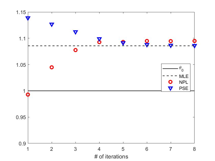
Figure 1: Compare MLE, NPL, and PSE

In contrast, the two-step approach generates a larger bias and standard error. Alternatively, we can take the sample average in the second step. However, the noise in nonparametric estimates near boundaries deteriorates the estimates substantially. The median performs much better the mean. It is clear that the performance of the two-step estimator is affected by the first-stage nonparametric regression.

Table 1: Monopoly Pricing: $\overline{x}=1$

	PSE	MLE	NPL	2-Step
mean	1.0052	1.0052	1.0059	0.9657
se	0.1201	0.1201	0.1209	0.1329

Remark 1.

This simple model has a convenient property that each firm’s optimal price is the solution of a strictly monotone function. In this case, the bisection method is fast and robust in solving the model, except that it takes many iterations to converge. In empirical games, the equilibrium is the solution of a system of nonlinear equations, which is harder to find and often lacks reliable algorithms.

3 Our Penalized Sieve Estimator

Now, we describe our estimator in detail. Instead of solving for $p^{*}(\theta)$ for each parameter $\theta$ in the likelihood evaluation, we approximate the true solution by $p^{\beta}$. The choice of approximation infrastructure depends on its approximation properties and computational convenience. A popular one often adopted in empirical studies is the method of sieves; that is, $p^{\beta}(\cdot)=\sum_{k=1}^{K}\beta_{k}s_{k}(\cdot)$, where $\{s_{1},\ldots,s_{K}\}$ represent the basis functions of the finite-dimensional sieve space $\mathcal{B}$. Typical choices of $s_{k}$ include B-spline basis functions and Bernstein polynomials. Such methods are flexible in accounting for shape restrictions imposed by the structural model, such as nonnegativityh and monotonicity. For instance, if $p$ represents choice probabilities, we can use $p^{\beta}(\cdot)=[1+\exp\{\sum_{k=1}^{K}\beta_{k}s_{k}(\cdot)\}]^{-1}$ to ensure that $p\in(0,1)$.

Moreover, our sieve estimator imposes the model restrictions by penalizing the difference between $p^{\beta}$ and $\Psi(p^{\beta},\theta)$. This difference is independent of the data sample in measuring the fidelity of approximation to the equilibrium conditions. The smaller the difference, the better the approximate $p^{\beta}$ satisfies equilibrium conditions.

We formulate the penalized log-likelihood criterion by combining the data fitting and model fitting criteria,

$$\underbrace{\ell\big{[}p^{\beta}(\cdot),\theta\big{]}}_{\ell(\beta,\theta)}-\omega\times\underbrace{\rho\Big{[}p^{\beta}(\cdot),\Psi\big{(}p^{\beta}(\cdot),\theta\big{)}\Big{]}}_{\rho(\beta,\theta)},$$ (3)

where $\omega>0$ is the smoothing parameter, and $\rho$ is a metric that measures the difference between $p^{\beta}$ and $\Psi(p^{\beta},\theta)$. For simplicity, we shall use as shorthand $\ell(\beta,\theta)$ and $\rho(\beta,\theta)$.

3.1 Estimation Algorithms

We propose several algorithms to implement our estimator given each smoothing parameter $\omega$: a joint algorithm and a nested algorithm.

Joint Algorithm This algorithm is attractive because it involves a single-level optimization problem. We augment the unknown to $(\beta,\theta)$ and solve the following problem:

$$\max_{\beta,\theta}\quad\ell(\beta,\theta)-\omega\times\rho(\beta,\theta),$$ (4)

which leads to $\widehat{\beta}(\omega)$ and $\widehat{\theta}(\omega)$. We recommend supplying an analytic gradient and Hessian to reduce computational cost and to increase precision.

Nested Algorithm This algorithm is intuitive, resembling MLE. There are two layers of optimization problems to be solved. In the inner layer, given $(\theta,\omega)$, we find the best approximation parameter $\widehat{\beta}(\theta;\omega)$ that solves the following problem:

$$\max_{\beta\in\mathbb{R}^{K}}\quad\ell(\beta,\theta)-\omega\times\rho(\beta,\theta).$$ (5)

Solving (5) indicates that the maximizer $\widehat{\beta}(\theta;\omega)$ is an implicit function of $\theta$.

In the outer layer, applying the best fitting approximation parameter, we search for the structure parameter $\widehat{\theta}(\omega)$ that maximizes the following likelihood:

$$\max_{\theta}\quad\ell\left(\widehat{\beta}(\theta,\omega),\theta\right).$$ (6)

Note that we have considered the structure equation (1) in the inner layer. Therefore, the equilibrium conditions are embedded in $\widehat{\beta}(\theta,\omega)$. As illustrated above, the optimizer of (5), $\widehat{\beta}(\theta;\omega)$, is an implicit function of $\theta$. Therefore, $\ell\left(\widehat{\beta}(\theta,\omega),\theta\right)$ in (6) is a function of $\theta$. We obtain the final estimator of $\theta$, denoted by $\widehat{\theta}(\omega)$, by directly maximizing (6) with respect to $\theta$.

Remark 2.

Because we solve the inner loop problem many times, it is more efficient to provide the gradient and Hessian of $h(\beta,\theta)=\ell(\beta,\theta)-\omega\rho(\beta,\theta)$ with respect to $\beta$, as well as the gradient of the objective function in the outer loop $\widehat{\ell}(\theta)=\ell(p^{\widehat{\beta}(\theta)}(\cdot),\theta)$ with respect to $\theta$. While the former is often straightforward, the latter is a bit more involved because the best-fitting approximation $\widehat{\beta}(\theta)$ is implicit. In particular, it requires deriving how the best-fitting approximation changes with respect to the model parameter, $\nabla\widehat{\beta}(\theta)$. Proposition A1 provides the gradient of the outer loop.

Alternatively, we can use an alternating iterative algorithm in place of either algorithm. That is, we can iterate the problem in (5) given a current estimate of $\theta$ and the problem in (6) to update the estimate of $\theta$. The iterations will continue until convergence. This iterative approach is similar to NPL.

The Choice of Tuning Parameters

We propose a new method that relies on the performance of parameter estimation to select the smoothing parameter $\omega$. In particular, we start with a moderate $\omega_{1}$ and update it till the estimates converge. For each $\omega=\omega_{\tau}$, we can conduct the joint or nested algorithm and obtain an estimate $\widehat{\theta}(\omega_{\tau})$. Consider a significance level of $\alpha$. We obtain its standard error $\widehat{\sigma}(\omega_{\tau})$ and confidence interval $\mathcal{I}(\omega_{\tau})=[\widehat{\theta}(\omega_{\tau})+z_{\alpha/2}\widehat{\sigma}(\omega_{\tau}),\widehat{\theta}(\omega_{\tau})+z_{1-\alpha/2}\widehat{\sigma}(\omega_{\tau})]$, applying the standard formula of standard error calculation for MLE.

We multiply the smoothing parameter by $T$ each time, i.e. $\omega_{\tau+1}=T\times\omega_{\tau}$ and obtain a new estimate and its confidence interval $\mathcal{I}(\omega_{\tau+1})$. Continue this process till the overlapping portion of the two intervals accounts for more than a threshold percentage of either of the two. That is, our final choice of the smoothing parameter is $\widehat{\omega}=\omega_{\tau}$ if and only if

$$\min\left\{\frac{|\mathcal{I}(\omega_{\tau})\cap\mathcal{I}(\omega_{\tau-1})|}{|\mathcal{I}(\omega_{\tau-1})|},\frac{|\mathcal{I}(\omega_{\tau})\cap\mathcal{I}(\omega_{\tau-1})|}{|\mathcal{I}(\omega_{\tau})|}\right\}\geq\mathfrak{c},$$

where $|\cdot|$ represents the length of the interval. In case the parameter of interest $\theta$ is multi-dimensional, we check this condition element by element. The final estimate of the model parameter follows $\widehat{\theta}(\widehat{\omega})$.

All the simulations reported in this paper adopt $\alpha=0.05$, $T=10$, and $\mathfrak{c}=95\%$. Therefore, $z_{\alpha/2}=-1.96$ and $z_{1-\alpha/2}=1.96$. To illustrate how the proposed method works in terms of selecting the tuning parameter, consider the monopoly pricing example with $x_{j}=1$. Figure 2 reports the parameter estimate and confidence intervals when the smoothing parameter varies. The x-axis represents $\log\omega$. While the bias seems small for small values of $\omega$, the confidence interval is large. As $\omega$ increases, it shrinks to the MLE confidence interval.

Figure 2: Choosing The Smoothing Parameter

Note: The data generating process is $y_{j}\sim\mathcal{N}(W(\theta_{0}),1)$, where $\theta_{0}=1$. This figure demonstrates how the penalized sieve estimate and its confidence interval change when the smoothing parameter increases.

The approximation parameter $K$ (i.e., the number of basis functions) should be chosen properly: large enough to approximate the equilibrium well. Exactly how many is sufficient depends on the complexity of the equilibrium solution. In our motivating example, the solution is simple; as a result, we find that four cubic basis functions are enough to approximate the solution well. When the solution is complex and the number of basis functions needs to be large, the analyst should start with a large smoothing parameter to avoid over-fitting in the inner loop; i.e., the likelihood function dominates. Sometimes, there are a finite number of states in the structural model, which is often assumed in estimating dynamic models. See, e.g., Aguirregabiria and Mira (2002) and Pesendorfer and Schmidt-Dengler (2008). Such finite states often come from discretization of covariates. In this case, the approximation can be perfect, i.e., $\beta=p$. That is, $s_{k}(x)=\mathbbm{1}(x=p_{k})$, where $\mathbbm{1}(\cdot)$ is the indicator function and $p_{k}$ is the $k$th element in the endogenous variable $p$. Note in this scenario the number of basis functions is identical to the dimensionality of $p$.

To capture empirically relevant covariates without losing much efficiency, any approximation methods would suffer from a computational curse of dimensionality — the total number of basis functions has to grow fast as the dimensionality of $p$ increases. We propose to resolve this issue in several ways. First, more advanced approximation methods are often preferable to simple ones. Additional shape constraints, sparsity patterns, and better grid choices are useful in reducing computational burden. See, e.g., Chen (2007) discusses various sieve-based methods and Kristensen et al. (2021) discuss various approximation architectures for approximating value functions in dynamic models. Second, there are also many model-specific techniques for approximating functions using a small number of basis functions. For instance, in static games of asymmetric information, if the deterministic component in the payoff function is linear in the parameters, see, e.g., Bresnahan and Reiss (1991) and Bajari et al. (2010), how covariates determine the endogenous variable becomes a multiple-index model. One can borrow techniques from the existing literature in estimating such a model.

3.2 Asymptotic Properties

As stated above, our proposed method can accommodate both continuous states leading to an infinite-dimensional endogenous variable $p$ like in Equation (2), and discrete states leading to a finite-dimensional $p$. In this paper we are concerned about the theoretical properties of the parameter estimator for the finite-dimensional case. The infinite-dimensional case deserves another paper; see footnote 4 below.

Let $p=(p_{1},\ldots,p_{d_{1}})^{\prime}\in\mathbb{R}^{d_{1}}$ be the endogenous variable in (1). Without loss of generality, we assume that $\theta\in\mathbb{R}^{d}$ and $\Theta$ denote the space of $\theta$. Moreover, we establish consistency and asymptotic normality of the joint estimator in the main text. The nested estimator is also consistent and asymptotically normal (see Theorems A2 and A3 in Appendix A.3). In fact, the two estimators have the same asymptotic distribution.

Assumption 1.

The parameter space $\Theta$ is a compact subset of $\mathbb{R}^{d}$.

For any given $\theta\in\Theta$, we aim to maximize the following function with respect to $p$

$$\ell_{n}(p)-\omega\|p-\Psi(p,\theta)\|_{2}^{2},$$ (7)

where $\ell_{n}$ denotes the log-likelihood corresponding to $n$ i.i.d. observations and $\|\cdot\|_{2}$ is the Euclidean norm. Suppose that $Y_{1},\ldots,Y_{n}$ are i.i.d. observations, taking values in $\mathbb{R}^{d_{2}}$. We assume that the likelihood function in (7) can be written as

$$\ell_{n}(p)=\frac{1}{n}\sum_{i=1}^{n}f(Y_{i},p),$$

where $f$ is a function defined on $\mathbb{R}^{d_{2}}\times\mathbb{R}^{d_{1}}$. For simplicity, we assume that $d_{2}=1$. In this context, $f(y,p)$ is actually the log density function of $Y_{i}$.

Assumption 2.

There exists a compact and convex set $K\subset\mathbb{R}^{d_{1}}$ such that $p$ must lie in $K$.

By Brouwer’s fixed-point theorem, there must exist a solution to (1) for any $\theta\in\Theta$. For instance, $p\in[0,1]$ represents CCP in dynamic games.

Define $g(p,\theta)=\Psi(p,\theta)-p$. Obviously, the solution to Equation (1), $p^{*}(\theta)$, satisfies $g(p^{*}(\theta),\theta)=0$. We impose the following regularity condition on $g(p,\theta)$.

Assumption 3.

There exists a positive constant $r$ such that for any $(p_{1},\theta),(p_{2},\theta)\in K\times\Theta$ satisfying $\|g(p_{1},\theta)\|_{2}\vee\|g(p_{2},\theta)\|_{2}\leq r$, we have $\|p_{1}-p_{2}\|_{2}\leq C\|g(p_{1},\theta)-g(p_{2},\theta)\|$ for some constant $C>0$.

Assumption 3 can be understood as a local inverse Lipschitz condition. Consider the Lambert function $p=W(\theta)$, which is defined implicitely by $pe^{p}=\theta$. In correspondence, $g(p,\theta)=\theta e^{-p}-p$. Thus, $(p+g)e^{p+g}=\theta e^{g}$, which implies that $p+g=W(\theta e^{g})$ or

$$p(g)=-g+W\left(\theta e^{g}\right).$$

Since $W$ is a continuously differentiable function by the implicit function theorem, for any $g_{1},g_{2}$ satisfying $|g_{1}|\vee|g_{2}|\leq r$ with some constant $r$, we have $|p(g_{1})-p(g_{2})|\leq C|g_{1}-g_{2}|$ for some constant $C$.

Assumption 4.

$\Psi$ is twice differentiable in both $p$ and $\theta$, and the Jacobian defined by $J_{g,p}(p,\theta)=\left[\frac{\partial g_{i}}{\partial p_{j}}(p^{*}(\theta),\theta)\right]$ is invertiable.

By the implicit function theorem, this assumption can guarantee that the solution to Equation (1), $p=p^{*}(\theta)$, is a continuously differentiable function of $\theta$.

Let $\theta_{0}$ denote the true value of $\theta$. Define

$$M(\theta)={\rm E}\,_{\theta_{0}}[f(Y_{i},p^{*}(\theta))]\quad\quad\text{for}~{}\theta\in\Theta,$$

where the expectation is taken with respect to $\mathbb{P}_{\theta_{0}}$.

Assumption 5.

The true value $\theta_{0}$ is in the interior of $\Theta$.

Assumption 6.

$M(\theta)$ is a continuous function and has a unique maximum at $\theta_{0}$ in $\Theta$.

This assumption ensures that the parameter $\theta_{0}$ is identifiable.

Assumption 7.

$f(y,p)\leq 0$ for any $(y,p)\in\mathbb{R}^{1+d_{1}}$ and $f(y,p)\in C(\mathbb{R}\times\mathbb{R}^{d_{1}})$. Moreover, if $Y_{i}$ is not bounded, $f(y,p)$ satisfies that for any compact set $D\subset\mathbb{R}^{d_{1}}$,

$$\liminf_{|y|\rightarrow\infty}\frac{1+\inf_{x\in D}[-f(y,p)]}{\sup_{p\in D}[-f(y,p)]}>0.$$

This assumption holds for square loss functions, i.e., $f(y,p)=-(y-p)^{2}$.

Given any $\theta\in\Theta$ and a positive $\omega$, recall

$$\hat{p}(\theta)=\operatorname*{arg\,max}_{p}\frac{1}{n}\sum_{i=1}^{n}f(Y_{i},p)-\omega\|p-\Psi(p,\theta)\|_{2}^{2}.$$ (8)

The following theorem indicates the approximate solution to the structure equation (1) is uniformly close to the exact solution $p^{*}(\theta)$.

Theorem 1.

Assume that Assumptions 1-7 are satisfied. Then, we have

$$\sup_{\theta\in\Theta}\|\hat{p}(\theta)-p^{*}(\theta)\|_{2}=O_{P}\left(\frac{1}{\sqrt{\omega_{n}}}\right),$$ (9)

provided that $\omega=\omega_{n}\rightarrow\infty$ as $n$ approaches infinity.

Remark 3.

The error term originates from using a finite $\omega$. Since $\omega$ is finite, the solution to the penalized optimization problem in (7) is affected by the sample through the likelihood function $\ell_{n}$. Therefore, there exist discrepancies between this estimator and the solution to the structural equation (1), which is the also the minimizer of the penalty term $\rho(p,\Psi(p,\theta))$ for any given $\theta$.

To establish the consistency of the estimator $\hat{\theta}_{n}$, we need a stronger version of Assumption 7.

Assumption 8.

$f(y,p)\leq 0$ for any $(y,p)\in\mathbb{R}^{1+d_{1}}$ and $f(y,p)\in C(\mathbb{R}\times\mathbb{R}^{d_{1}})$ satisfying

$${\rm E}\,_{\theta_{0}}\left[\left\|\frac{\partial f}{\partial p}(Y_{i},p^{*}(\theta_{0}))\right\|_{2}\right]<\infty.$$

Moreover, if $Y_{i}$ is not bounded, $f(y,p)$ satisfies that for any compact set $D\subset\mathbb{R}^{d_{1}}$,

$$\liminf_{|y|\rightarrow\infty}\frac{1+\inf_{p\in D}[-f(y,p)]}{\sup_{p\in D}[-f(y,p)]}>0~{}~{}\text{and}~{}~{}\liminf_{|y|\rightarrow\infty}\frac{1+\inf_{p\in D}|\partial f(y,p)/\partial p_{j}|}{\sup_{p\in D}|\partial f(y,p)/\partial p_{j}|}>0$$

for $j=1,\ldots,d_{1}$.

Let $\tilde{\theta}_{n}$ denote the estimator of $\theta$ obtained from the joint algorithm. Actually, $\tilde{\theta}_{n}$ is defined by

$$\tilde{\theta}_{n}=\operatorname*{arg\,max}_{\theta\in\Theta}\ell_{n}(\hat{p}(\theta))-\omega\|\hat{p}(\theta)-\Psi(\hat{p}(\theta),\theta)\|_{2}^{2},$$ (10)

where $\hat{p}(\theta)$ is given by (8).

Theorem 2.

Suppose that Assumptions 1-6 and 8 hold. If $\omega=\omega(n)\rightarrow\infty$, then $\tilde{\theta}_{n}$ is consistent.

Remark 4.

Since $\tilde{\theta}_{n}$ is the maximizer of $\ell_{n}(\hat{p}(\theta))$ with a non-positive penalty, we choose $\ell_{n}(\hat{p}(\theta))$ as the criterion function. Though it is difficult to evaluate the gradient of $\hat{p}(\theta)$ with respect to $\theta$, we can still use it as our criterion function, because we have established the bound on the difference between $\hat{p}(\theta)$ and $p^{*}(\theta)$ in Theorem 1. We establish the consistency and the asymptotic normality of $\tilde{\theta}_{n}$ by resorting to the techniques for $M$-estimators. Even though $\tilde{\theta}_{n}$ is not the maximizer of $\ell_{n}(p^{*}(\theta))$, we are able to control the difference between $\ell_{n}(p^{*}(\tilde{\theta}_{n}))$ and $\max_{\theta\in\Theta}\ell_{n}(p^{*}({\theta}))$. We show that, in actuality, $\tilde{\theta}_{n}$ nearly maximizes $\ell_{n}(p^{*}({\theta}))$, and then we leverage the results for $M$-estimators; see Section 5.2 of Van der Vaart and Wellner (1996) for more details.

To derive asymptotic normality, we need a stronger condition than Assumptions 7 and 8.

Assumption 9.

$f(y,p)\leq 0$ for any $(y,p)\in\mathbb{R}^{1+d_{1}}$ and $f(y,p)\in C(\mathbb{R}\times\mathbb{R}^{d_{1}})$ satisfying

$${\rm E}\,_{\theta_{0}}\left[\left\|\frac{\partial f}{\partial p}(Y,p^{*}(\theta_{0}))\right\|_{2}^{2}\right]<\infty\quad\text{and}\quad{\rm E}\,_{\theta_{0}}\left[\left|\frac{\partial^{2}f}{\partial p_{i}\partial p_{j}}(Y,p^{*}(\theta_{0}))\right|\right]<\infty$$

for $i,j=1,\ldots,d_{1}$. Moreover, if $Y_{i}$ is not bounded, $f(y,p)$ satisfies that for any compact set $D\subset\mathbb{R}^{d_{1}}$,

$$\liminf_{|y|\rightarrow\infty}\frac{1+\inf_{p\in D}[-f(y,p)]}{\sup_{p\in D}[-f(y,p)]}>0~{}~{}~{}~{}\liminf_{|y|\rightarrow\infty}\frac{1+\inf_{p\in D}|\partial f(y,p)/\partial p_{j}|}{\sup_{p\in D}|\partial f(y,p)/\partial p_{j}|}>0$$

for $j=1,\ldots,d_{1}$, and

$$\liminf_{|y|\rightarrow\infty}\frac{1+\inf_{p\in D}|\partial^{2}f(y,p)/\partial p_{i}\partial_{j}|}{\sup_{p\in D}|\partial^{2}f(y,p)/\partial p_{i}\partial p_{j}|}>0$$

for any $i,j=1,\ldots,d_{1}$.

Theorem 3.

Suppose that Assumptions 1-6 and 9 hold. If $\omega_{n}/n^{2}\rightarrow\infty$ and the matrix

$$V_{\theta_{0}}={\rm E}\,_{\theta_{0}}\left[\left\{\frac{\partial p^{*}(\theta_{0})}{\partial\theta}\right\}^{\prime}\frac{\partial^{2}f(Y_{i},p^{*}(\theta_{0}))}{\partial p\partial p^{\prime}}\left\{\frac{\partial p^{*}(\theta_{0})}{\partial\theta}\right\}\right]$$

is invertible, then

$$\sqrt{n}\,(\tilde{\theta}_{n}-\theta_{0})\overset{d}{\to}\mathcal{N}(0,\Sigma),$$

where $\Sigma=V_{\theta_{0}}^{-1}\left(\frac{\partial p^{*}(\theta_{0})}{\partial\theta}\right)^{\prime}{\rm E}\,_{\theta_{0}}\left[\left\{\frac{\partial f(y,p^{*}(\theta_{0}))}{\partial p}\right\}\left\{\frac{\partial f(y,p^{*}(\theta_{0}))}{\partial p}\right\}^{\prime}\right]\left(\frac{\partial p^{*}(\theta_{0})}{\partial\theta}\right)V_{\theta_{0}}^{-1}.$

Remark 5.

Under mild regularity conditions on $f$,

$$-{\rm E}\,_{\theta_{0}}\left[\frac{\partial^{2}f(Y_{i},p^{*}(\theta_{0}))}{\partial p\partial p^{\prime}}\right]={\rm E}\,_{\theta_{0}}\left[\left\{\frac{\partial f(y,p^{*}(\theta_{0}))}{\partial p}\right\}\left\{\frac{\partial f(y,p^{*}(\theta_{0}))}{\partial p}\right\}^{\prime}\right],$$

then $\Sigma=-V_{\theta_{0}}^{-1}$. Consequently, even though $\tilde{\theta}_{n}$ is different from the maximum likelihood estimator of $\theta$, which minimizes $\ell_{n}(p^{*}(\theta))$, the asymptotic variance of $\hat{\theta}_{n}$ attains the Cramér-Rao lower bound. Thus, $\tilde{\theta}_{n}$ is asymptotically efficient.

The joint algorithm is attractive because it involves a single-level optimization problem and computes the Hessian matrix with respect to $(\beta,\theta)$ at the solution directly. The following corollary provides a natural way to calculate the standard error of $\tilde{\theta}_{n}$ using the Hessian matrix generated from the joint algorithm.

Corollary 3.1.

The Fisher information can be characterized as

$$\widehat{H}=\bf{H}_{\theta\theta}-\bf{H}_{\beta\theta}^{\prime}\bf{H}_{\beta\beta}^{-1}\bf{H}_{\beta\theta},$$

where the matrices in bold are the four blocks in the Hessian matrix generated from a joint maximization algorithm,

$$\begin{bmatrix}\bf{H}_{\beta\beta}&\bf{H}_{\beta\theta}\\ \bf{H}_{\theta\beta}&\bf{H}_{\theta\theta}\end{bmatrix}.$$

3.3 Discussion

Case 1. $\omega=\infty$: We now discuss the extreme case when we let $\omega=\infty$. That is, for each guess of the model parameter $\theta$, we find the best approximation to minimize any deviation from the equilibrium condition and then evaluate the likelihood by plugging in this best approximation. Specifically, our estimator becomes equivalent to

$$\max_{\theta} \quad\ell(p^{\beta(\theta)},\theta;\text{data})$$

where $$\quad\beta(\theta)=\arg\min_{\beta}\rho(p^{\beta},\Psi(p^{\beta},\theta)),$$

which looks similar to MLE, with an important difference that we only search for the best approximation in the inner loop. We call this special case of our estimator the approximate MLE (AMLE).

One may wonder about the advantages of gradually changing $\omega$ instead of directly considering the limiting case. AMLE ignores the data when finding the best approximation of the solution for each $\theta$. Because the data are informative about the true strategies $p$, our general penalized sieve estimator may perform better than AMLE. By gradually updating the smoothing parameter, we shift the weight from the data to the equilibrium condition. At the minimum, a preliminary nonparametric estimate of $\widehat{p}$ (by letting $\omega=0$) constitutes a good starting value for the inner loop but is subject to issues with nonparametric estimates. When the smoothing parameter increases, more weight is given to the equilibrium condition. By forcing model restrictions more strongly, the estimates converge to MLE estimates.

Case 2. $\omega=\infty$ and $\beta=p$: Our method could incorporate each element of the endogenous variable $p$ as a basis function in sieve approximation and put all of the weight on the equilibrium conditions in the inner loop. As a result, our estimator covers the MPEC estimator as a special case. Our above-mentioned derivation also suggests a natural way to calculate standard errors for MPEC estimators.

Corollary 3.2.

When $\omega=\infty$ and $\beta=p$, the observed Fisher information can be characterized as

$$\bf{\widehat{H}}=\bf{H}_{\theta\theta}+[\nabla\widehat{\beta}(\widehat{\theta})]^{\prime}\bf{H}_{\beta\beta}[\nabla\widehat{\beta}(\widehat{\theta})]+[\nabla\widehat{\beta}(\widehat{\theta})]^{\prime}\bf{H}_{\beta\theta}+[\bf{H}_{\beta\theta}]^{\prime}\nabla\widehat{\beta}(\widehat{\theta}),$$

where $\nabla\beta(\widehat{\theta})=-\left[\nabla_{\beta}g\right]^{-1}\times\nabla_{\theta}g$ on the right-hand side, and the matrices in bold are the four blocks in the Hessian matrix generated from a constrained maximization algorithm,

$$\begin{bmatrix}\bf{H}_{\beta\beta}&\bf{H}_{\beta\theta}\\ \bf{H}_{\theta\beta}&\bf{H}_{\theta\theta}\end{bmatrix}.$$

To the best of our knowledge, this result is new in the literature. Su and Judd (2012) suggest obtaining standard errors through bootstrapping. We derive the general result in Section 3.2. Here, we consider $p,\beta,\theta\in\mathbb{R}$, as in the simple example with $x_{j}=1$, to explain the idea. When $\omega=\infty$ and $\beta=p$, our estimator is effectively an MPEC estimator,

$$\max_{g(\beta,\theta)=0}\quad\ell(\beta,\theta).$$

The MPEC approach forms the Lagrangian function $h(\beta,\theta,\omega)=\ell(\beta,\theta)+\lambda g(\beta,\theta)$. Note that this multiplier $\lambda$ should not to be confused with the smoothing parameter $\omega$ for general PSE. By definition, we have $g(\widehat{\beta}(\theta),\theta)=0$. Its first-order and second-order derivatives are

$$g_{\scriptscriptstyle\beta}\widehat{\beta}^{\prime}(\theta)+g_{\scriptscriptstyle\theta} =0$$

$$g_{\scriptscriptstyle\beta\beta}[\widehat{\beta}^{\prime}(\theta)]^{2}+2g_{\scriptscriptstyle\beta\theta}\widehat{\beta}^{\prime}(\theta)+g_{\scriptscriptstyle\beta}\widehat{\beta}^{\prime\prime}(\theta)+g_{\scriptscriptstyle\theta\theta} =0,$$

which allow for expressing $\widehat{\beta}^{\prime}(\theta)$ and $\widehat{\beta}^{\prime\prime}(\theta)$ in the gradient of $g$.

On the other hand, the second-order derivative of the likelihood is

$$\widehat{\ell}_{\theta\theta}(\theta)|_{\theta=\widehat{\theta}} =\ell_{\beta\beta}[\widehat{\beta}^{\prime}(\theta)]^{2}+2\ell_{\beta\theta}\widehat{\beta}^{\prime}(\theta)+\ell_{\beta}\widehat{\beta}^{\prime\prime}(\theta)+\ell_{\theta\theta}$$

$$=\Big{[}\left(\frac{g_{\scriptscriptstyle\theta}}{g_{\scriptscriptstyle\beta}}\right)^{2}(\ell_{\beta\beta}+\lambda g_{\scriptscriptstyle\beta\beta})-2\frac{g_{\scriptscriptstyle\theta}}{g_{\scriptscriptstyle\beta}}(\ell_{\beta\theta}+\lambda g_{\scriptscriptstyle\beta\theta})+(\ell_{\theta\theta}+\lambda g_{\scriptscriptstyle\theta\theta})\Big{]}\bigg{|}_{\beta=\widehat{\beta}(\widehat{\theta}),\theta=\widehat{\theta}},$$

where $\lambda$ denotes the associated Lagrange multiplier reported by a constrained maximization algorithm. The last equation follows from the Lagrange multiplier theorem that $\ell_{\beta}+\lambda g_{\scriptscriptstyle\beta}=0$ at the optimum $(\beta=\widehat{\beta}(\widehat{\theta}),\theta=\widehat{\theta})$ and the first-order and second-order derivatives of the equilibrium constraints. All terms on the RHS are readily available if MPEC converges. We recommend supplying the analytic gradient and Hessian, as the numerical one can be inaccurate.

4 Application: Walmart versus Kmart Entry Game

In this section, we apply our methodology to study an entry game between Walmart and Kmart. Specifically, we draw on a dataset published by Jia (2008) that studies the discount retail industry. To illustrate our method, we use a simplified version of the model and only a subset of the collected variables. A detailed description of the industry and data can be found in the original paper.

4.1 Data

The original data contain 2,065 markets, each of which is a county with an average population between 5 to 64 thousands, between the years 1988 - 1997. A simple scatter plot of the total number of firms, as in Figure 3, reveals that neither firm enters the market when sales per capita (SPC) is too small. Given the lack of activity in these markets, we restrict the analysis to SPC of at least 7.25, which represents the minimum SPC where at least one firm enters. We will use SPC as our main explanatory variable and focus on the year 1997 in our analysis.

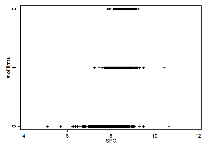
Figure 3: Total Number of Firms

Denote the data as $\{d_{\mathcal{W}m},d_{\mathcal{K}m},x_{m}\}_{m=1}^{M}$, where $d_{jm}$ is firm $j$’s entry decision in market $m$, and $x_{m}$ is the SPC in this market. Table 2 shows some summary statistics of the sample we use (bottom panel) and the original sample (top panel). Because we are dropping only 68 markets out of 2,065, the summary statistics are quite similar. On the other hand, the range of SPC declines from $5.58$ to $3.41$, which makes our analysis much more focused.

Table 2: Summary Statistics

Variable	Obs	Mean	Std. Dev.	Min	Max
Walmart	2,065	0.4755	0.4995	0	1
Kmart		0.1903	0.3926	0	1
SPC		8.2024	0.4670	5.08	10.66
Walmart	1,997	0.4917	0.5001	0	1
Kmart		0.1968	0.3977	0	1
SPC		8.2453	0.4061	7.25	10.66

4.2 Empirical Model

For the purpose of illustrating our method, we model the entry game between Walmart and Kmart as a static game with incomplete information. Two players, Walmart ($\mathcal{W}$) and Kmart ($\mathcal{K}$), decide whether to enter a market. We assume that they make independent decisions across markets. Let $d_{j}=1$ if firm $j$ is active and $0$ otherwise. The payoff function of firm $j$ depends on its own productivity, whether its competitor enters or not, market-specific covariates, and private information:

$$u_{j}(d_{j},d_{-j})=\pi_{j}-d_{-j}\Delta_{j}+\gamma x+\epsilon_{j1}$$

if $d_{j}=1$ and $=\epsilon_{j0}$ otherwise, where $\theta=(\pi_{\mathcal{W}},\Delta_{\mathcal{W}},\pi_{\mathcal{K}},\Delta_{\mathcal{K}},\gamma)^{\prime}$, market characteristics $x$ are common knowledge, and firm $j$’s private information $\epsilon_{j}$ is type-1 extreme value distributed and independent of $\epsilon_{-j}$. Firm $j$’s profit is $\pi_{j}$ under monopoly and $\pi_{j}-\Delta_{j}$ under duopoly. Note we allow asymmetry in business-stealing effects; i.e., the presence of the competing firm has different effects on the two firms. The term $\gamma x$ determines the market-specific payoff.

Therefore, the probability that firm $j$ chooses to enter is

$$p_{j}=\frac{1}{1+\exp\left\{-\pi_{j}-\gamma x+p_{-j}\Delta_{j}\right\}},$$

where $p_{-j}$ is its competitor’s entry probability. Denote the conditional choice probabilities (CCP hereafter) as $p=(p_{\mathcal{W}},p_{\mathcal{K}})^{\prime}$. Define a best response mapping from CCP to CCP $\Psi:p\rightarrow p$. In equilibrium, we must have

$$p=\Psi(p,\theta).$$

4.3 Estimation Results

To approximate the CCPs, we use cubic basis functions (see Appendix A.5):

$$p_{j}^{\beta}(\cdot)=\frac{1}{1+\exp\{\sum\beta_{jk}s_{k}(\cdot)\}},$$

where $s_{k}(\cdot)$ is a cubic basis function and $\beta=(\beta_{\mathcal{W}1},\ldots,\beta_{\mathcal{W}K},\beta_{\mathcal{K}1},\ldots,\beta_{\mathcal{K}K})^{\prime}$. This is equivalent to approximating the ex-ante value of entry, before observing T1EV errors, by $\sum\beta_{jk}s_{k}(\cdot)$. We try different numbers of basis functions.

We define the likelihood function as

$$\ell(p^{\beta},\theta)=\sum_{j=\mathcal{W},\mathcal{K}}\sum_{m=1}^{M}\left[d_{jm}\log\left(p_{j}^{\beta}(x_{m})\right)+(1-d_{jm})\log\left(1-p_{j}^{\beta}(x_{m})\right)\right]$$

and the penalization as

$$\rho(\beta,\theta)=\sum_{j=\mathcal{W},\mathcal{K}}\sum_{m=1}^{M}\left[p_{j}^{\beta}(x_{m})-\Psi_{j}\left(p_{-j}^{\beta}(x_{m}),\theta\right)\right]^{2},$$

which accounts for the equilibrium conditions for the set of observed market-specific covariates. In addition, we supply analytic gradient and Hessian; see Appendix A.4.2.

Table 3 shows the estimated parameters when the number of basis functions, $K$, varies from 6 to 8. When there is a lack of statistical significance, the estimate varies when $K$ changes. In contrast, the estimate is quite stable when it is significant. As expected, entry is more likely in markets with large retail SPC.

Table 3: Estimation Results

	$\widehat{\theta}$	se	$\widehat{\theta}$	se	$\widehat{\theta}$	se
$\pi_{\mathcal{W}}$	-20.65	1.19	-20.24	1.20	-20.23	1.20
$\Delta_{\mathcal{W}}$	0.50	0.28	0.35	0.26	0.28	0.24
$\pi_{\mathcal{K}}$	-23.55	0.98	-23.16	0.99	-23.14	1.00
$\Delta_{\mathcal{K}}$	-1.95	0.66	-2.04	0.65	-2.05	0.64
$\gamma$	2.51	0.15	2.46	0.15	2.45	0.15
$K$	8		7		6
$\ell(\widehat{\beta},\widehat{\theta})$	2012.22		2012.21		2012.14

Fix the number of basis functions at $K=8$. Figure 4 shows how the estimated parameters (dashed black lines) and the associated $95\%$ confidence intervals (red dotted lines) change when th smoothing parameter $\omega$ increases from $10$ to $10^{10}$. When the smoothing parameter is small, less weight is imposed on the equilibrium conditions, leading to biased estimates and wide confidence intervals. When this parameter is sufficiently large, the parameter estimates and the associated confidence intervals converge. Although the precise point at which we stop the algorithm depends on the choice of significance level $\alpha$, it appears that the estimates barely move when $\omega$ is higher than $10^{5}$.

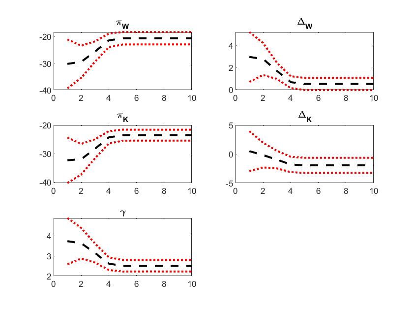
Figure 4: Estimated Parameters with Varying $\omega$

Figure 5 shows the estimated choice probabilities and demonstrates the fitness of the estimated model. The thin dashed lines represent the estimated choice probabilities, where blue represents Walmart and red represents Kmart. The thick lines represent the corresponding best responses with the estimated parameters. First, it is clear that the best responses coincide with the estimated choice probabilities, indicating an excellent model fit. That is, the estimated choice probabilities satisfy the equilibrium conditions. Naturally, the entry probability is increasing in SPC as the estimated $\widehat{\gamma}$ suggests. Second, Walmart enters with a higher probability in all markets. It is consistent with the estimates that, all else equal, Walmart benefits more from entry; i.e., $\pi_{\mathcal{W}}>\pi_{\mathcal{K}}$.

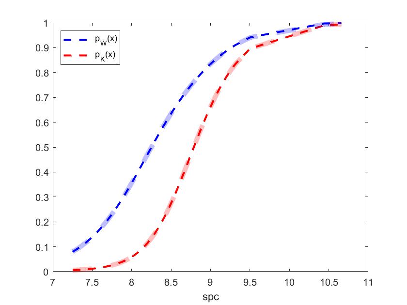
Figure 5: Estimated Choice Probabilities

5 Conclusion

A structural model builds on economic theory and describes how endogenous variables are related to a group of explanatory variables. Such relation is often an implicit function that depends on unknown parameters, which is costly to solve. Two-step methods avoid solving the model but rely on the performance of first-step estimation. We propose Penalized Sieve Estimators (PSE) as a new class of estimators, that rely on a sieve to approximate the solution and penalize deviation from the equilibrium condition. PSEs are easy to apply, at least as fast as alternative approaches that obtain MLE, and more robust in applications to various models. We expect our method to become a useful tool in structural estimation.

Appendix A Appendix

A.1 Optimal Monopoly Pricing With Logit Demand

In this subsection, we derive Equation (2). Rearranging terms gives $\xi_{j}-\alpha P_{j}+\exp(\xi_{j}-\alpha P_{j})=\xi_{j}-\alpha c_{j}-1$, which reduces to

$$\xi_{j}(x)-P_{j}^{*}(x)+\exp(\xi_{j}(x)-P_{j}^{*}(x))=\xi_{j}(x)-1$$

under our assumptions $c_{j}=0,\alpha=1$. Denote $M(x)=\exp(\xi_{j}(x)-P_{j}^{*}(x))$. The FOC can be rewritten as $\log M(x)+M(x)=\xi_{j}(x)-1$. Therefore, we have

$$M(x)=W(\exp(\xi_{j}(x)-1)),$$

applying an alternative definition of the Lambert W function $\log W(v)+W(v)=\log v$. That is, the optimal price satisfies

$$P_{j}^{*}(x)=\xi_{j}(x)-\log M(x)=\xi_{j}(x)-(\xi_{j}(x)-1-M(x))=1+W(\theta x),$$

where the first equation follows the definition of $M(\cdot)$, the second equation follows the rewritten FOC, and the last equation follows $\xi_{j}(x)=\log x+\log\theta+1$.

A.2 Proofs in Section 3.2

Proof of Theorem 1.

Define $\mathbb{P}_{n}f(Y,p)=\frac{1}{n}\sum_{i=1}^{n}f(Y_{i},p)$. To continue the proof, we first show the following technical result:

$$\sup_{\theta\in\Theta}\mathbb{P}_{n}[-f(Y,p^{*}(\theta))]=O_{p}(1).$$ (A1)

As Assumption 2 is met, $\|p^{*}(\theta)\|_{2}\leq C$ for some positive constant $C$ for any $\theta\in\Theta$. If $Y_{i}$ are bounded, $\sup_{\theta\in\Theta}\mathbb{P}_{n}[-f(Y,p^{*}(\theta))]$ must be bounded, because $f$ is a continuous function. Hence, the result holds. If $Y_{i}$ are not bounded, according to Assumption 7, there exists a positive constant $\eta$ such that

$$\eta\sup_{x\in K}[-f(y,x)]\leq 1+\inf_{x\in K}[-f(y,x)]\quad\forall y\in\mathbb{R}.$$

Therefore,

$$\sup_{\theta\in\Theta}\mathbb{P}_{n}[-f(Y,p^{*}(\theta)]\leq\eta^{-1}(1+\mathbb{P}_{n}[-f(Y,p^{*}(\theta_{0}))].$$

By the strong law of large numbers, with probability one, we have

$$\mathbb{P}_{n}[-f(Y,p^{*}(\theta_{0}))]\rightarrow{\rm E}\,_{\theta_{0}}[-f(Y,p^{*}(\theta_{0}))]=-M(\theta_{0})<\infty.$$

It follows that $\eta^{-1}\{1+\mathbb{P}_{n}[-f(Y,p(\theta_{0}))]\}=O_{p}(1)$. Equation (A1) is established.

Let $J(p,\theta)=\|p-\Psi(p,\theta)\|_{2}^{2}$. Based on the definition of $\hat{p}(\theta)$, we have that, for any $\theta\in\Theta$,

$$\ell_{n}(\hat{p}(\theta))-\omega_{n}J(\hat{p}(\theta),\theta)\geq\ell_{n}(p^{*}(\theta)).$$

As $\ell_{n}(\hat{p}(\theta))\leq 0$ by Assumption 7, it follows that

$$-\omega_{n}J(\hat{p}(\theta),\theta)\geq\ell_{n}(p^{*}(\theta)).$$

Then,

$$J(\hat{p}(\theta),\theta) \leq-\omega_{n}^{-1}\ell_{n}(p^{*}(\theta))=\omega_{n}^{-1}\mathbb{P}_{n}[-f(Y,p^{*}(\theta))].$$

Therefore, we have $\sup_{\theta\in\Theta}J(\hat{p}(\theta),\theta)=\omega_{n}^{-1}O_{p}(1)$. It gives rise to

$$\sup_{\theta\in\Theta}\|g(\hat{p}(\theta),\theta)\|_{2}=O_{P}\left(\frac{1}{\sqrt{\omega_{n}}\,}\right),$$

while $g(p^{*}(\theta),\theta)=0$. By Assumption 3, we have

$$\sup_{\theta\in\Theta}\|\hat{p}(\theta)-p^{*}(\theta)\|_{2}\leq O_{P}\left(\frac{1}{\sqrt{\omega_{n}}}\right).$$

This completes the proof. ∎

Proof of Theorem 2.

We first show that

$$\sup_{\theta\in\Theta}|\ell_{n}(\hat{p}(\theta))-\ell_{n}(p^{*}(\theta))|=O_{P}\left(\frac{1}{\sqrt{\omega_{n}}}\right)+o_{P}\left(\frac{1}{n}\right).$$ (A2)

Recall that $M(\theta)={\rm E}\,_{\theta_{0}}[f(Y_{i},p^{*}(\theta))]$. Then, we define

$$M_{n}(\theta)=\ell_{n}(p^{*}(\theta))=\frac{1}{n}\sum_{i=1}^{n}f(Y_{i},p^{*}(\theta))\quad\text{for}~{}\theta\in\Theta.$$

We will show

$$\sup_{\theta\in\Theta}|M_{n}(\theta)-M(\theta)|=o_{P}(1).$$ (A3)

Finally, we prove that

$$\tilde{\theta}_{n}\rightarrow\theta_{0}$$

in probability as $n\rightarrow\infty$.

To prove (A2), we assume that $\Theta$ is convex without loss of generality. By Assumption 2, there must exist some positive constant $T$ such that

$$\|p^{*}(\theta)\|_{2}\leq T,\quad\quad\forall\theta\in\Theta.$$

Let $V_{n}=\sup_{\theta\in\Theta}\|\hat{p}(\theta)-p^{*}(\theta)\|_{2}$. Theorem 1 indicates

$$V_{n}\leq O_{p}\left(\frac{1}{\sqrt{\omega_{n}}}\right).$$

By Assumption 8, there exists a positive constant $\eta$ such that, for $j=1,\ldots,d_{1}$,

$$\sup_{\|p\|_{2}\leq T+1}\left|\frac{\partial f}{\partial p_{j}}(y,p)\right|\leq\frac{1}{\eta}\left(1+\inf_{\|p\|_{2}\leq T+1}\left|\frac{\partial f}{\partial p_{j}}(y,p)\right|\right)\quad\forall y\in\mathbb{R}.$$ (A4)

Then, it follows that

$$\quad\quad|\ell_{n}(\hat{p}(\theta))-\ell_{n}(p^{*}(\theta))|$$

$$\leq\frac{1}{n}\sum_{i=1}^{n}|f(Y_{i},\hat{p}(\theta))-f(Y_{i},p^{*}(\theta))|$$

$$=\frac{1}{n}\sum_{i=1}^{n}|f(Y_{i},\hat{p}(\theta))-f(Y_{i},p^{*}(\theta))|\mathbbm{1}_{(V_{n}\leq 1)}+\frac{1}{n}\sum_{i=1}^{n}|f(Y_{i},\hat{p}(\theta))-f(Y_{i},p^{*}(\theta))|\mathbbm{1}_{(V_{n}>1)}$$

$$\leq\frac{1}{n}\sum_{i=1}^{n}\left[\sup_{\begin{subarray}{c}\|p\|_{2}\leq T+1,\\ 1\leq j\leq d_{1}\end{subarray}}\left|\frac{\partial f}{\partial p_{j}}(Y_{i},p)\right|\right]\|\hat{p}(\theta)-p^{*}(\theta)\|_{2}\mathbbm{1}_{(V_{n}\leq 1)}$$

$$\qquad\qquad\qquad+\frac{1}{n}\sum_{i=1}^{n}|f(Y_{i},\hat{p}(\theta))-f(Y_{i},p^{*}(\theta))|\mathbbm{1}_{(V_{n}>1)}$$

$$\leq\frac{1}{n}\sum_{i=1}^{n}\frac{1}{\eta}\left(1+\max_{1\leq j\leq d_{1}}\inf_{\|p\|_{2}\leq T+1}\left|\frac{\partial f}{\partial p_{j}}(Y_{i},p)\right|\right)V_{n}\mathbbm{1}_{(V_{n}\leq 1)}$$

$$\qquad\qquad\qquad+\frac{1}{n}\sum_{i=1}^{n}|f(Y_{i},\hat{p}(\theta))-f(Y_{i},p^{*}(\theta))|\mathbbm{1}_{(V_{n}>1)}$$

$$\leq\frac{1}{n}\sum_{i=1}^{n}\frac{1}{\eta}\left(1+\left\|\frac{\partial f}{\partial p}(Y_{i},p^{*}(\theta_{0}))\right\|_{2}\right)V_{n}+\frac{1}{n}\sum_{i=1}^{n}|f(Y_{i},\hat{p}(\theta))-f(Y_{i},p^{*}(\theta))|\mathbbm{1}_{(V_{n}>1)}.$$

Therefore,

$$\sup_{\theta\in\Theta}|\ell_{n}(\hat{p}(\theta))-\ell_{n}(p^{*}(\theta))|\leq \frac{1}{n}\sum_{i=1}^{n}\frac{1}{\eta}\left(1+\left\|\frac{\partial f}{\partial p}(Y_{i},p^{*}(\theta_{0}))\right\|_{2}\right)V_{n}$$ (A5)

$$\quad\quad+\frac{1}{n}\sum_{i=1}^{n}|f(Y_{i},\hat{p}(\theta))-f(Y_{i},p^{*}(\theta))|\mathbbm{1}_{(V_{n}>1)}.$$

By the strong law of large numbers and Assumption 8,

$$\frac{1}{n}\sum_{i=1}^{n}\left[1+\left\|\frac{\partial f}{\partial p}(Y_{i},p^{*}(\theta_{0}))\right\|_{2}\right]\rightarrow 1+{\rm E}\,_{\theta_{0}}\left\|\frac{\partial f}{\partial p}(Y_{i},p^{*}(\theta_{0}))\right\|_{2}$$

almost surely. So, it is $O_{P}(1)$. The second term on the right-hand side of (A5) is nonzero only in the event $\{V_{n}>1\}$, whose probability converges to zero by Theorem 1, so it is $o_{P}(n^{-1})$. Hence, we have established Equation (A2). Equation (A3) follows from Lemma A1, which will be presented later.

Now, we are ready to prove $\tilde{\theta}_{n}\rightarrow\theta_{0}$ in probability. Let $\delta$ be an arbitrary positive number. Assumption 6 indicates that $\theta_{0}$ is the unique maximizer of $M(\theta)$. As $M(\theta)$ is continuous over the compact set $\Theta$,

$$\gamma:=M(\theta_{0})-\sup_{\theta\in\Theta,d(\theta,\theta_{0})\geq\delta}M(\theta)>0,$$ (A6)

where $d(\theta,\theta_{0})=\|\theta-\theta_{0}\|_{2}$ for any $\theta\in\Theta$. Note that $\hat{\theta}_{n}\in\Theta$. By (A2) and (A3), we have

$$\quad\quad M(\theta_{0})-M(\tilde{\theta}_{n})$$

$$=M_{n}(\theta_{0})-M_{n}(\tilde{\theta}_{n})+o_{P}(1)$$

$$=\ell_{n}(p^{*}(\theta_{0}))-\ell_{n}(p^{*}(\tilde{\theta}_{n}))+o_{P}(1)$$

$$\leq\ell_{n}(p^{*}(\theta_{0}))-\ell_{n}(\hat{p}(\tilde{\theta}_{n}))+\sup_{\theta\in\Theta}|\ell_{n}(\hat{p}(\theta))-\ell_{n}(p^{*}(\theta))|+o_{P}(1)$$

$$=\ell_{n}(p^{*}(\theta_{0}))-\ell_{n}(\hat{p}(\tilde{\theta}_{n}))+o_{P}(1).$$

By definition of $\tilde{\theta}_{n}$ and $p^{*}(\theta_{0})$, we have

$$\ell_{n}(\hat{p}(\tilde{\theta}_{n}))\geq\ell_{n}(p^{*}(\theta_{0})),$$

so $M(\theta_{0})-M(\hat{\theta}_{n})\leq o_{P}(1)$. By (A6), one has

$$\{d(\tilde{\theta}_{n},\theta_{0})\geq\delta\}\subset\{M(\theta_{0})-M(\tilde{\theta}_{n})\geq\gamma\}\subset\{o_{P}(1)\geq\gamma\}.$$

Therefore,

$$\mathbb{P}_{\theta_{0}}(d(\tilde{\theta}_{n},\theta_{0})\geq\delta)\leq\mathbb{P}_{\theta_{0}}(o_{P}(1)\geq\gamma),$$

which converges to 0 as $n$ approaches infinity. As $\delta$ is an arbitrary positive number, $\tilde{\theta}_{n}$ is a consistent estimator of $\theta_{0}$. This completes the proof. ∎

Proof of Theorem 3.

We will mainly follow Theorem 5.23 of Van der Vaart (2000) to prove asymptotic normality of $\hat{\theta}_{n}$. Firstly, as we have shown in the proof of Lemma A1,

$$\quad\quad|f(y,p^{*}(\theta_{1}))-f(y,p^{*}(\theta_{2}))|$$

$$\leq\frac{1}{\eta}\left[1+\left\|\frac{\partial f}{\partial p}(y,p^{*}(\theta_{0}))\right\|_{2}\right]\|p^{*}(\theta_{1})-p^{*}(\theta_{2})\|_{2}$$

$$\leq\frac{C}{\eta}\left[1+\left\|\frac{\partial f}{\partial p}(y,p^{*}(\theta_{0}))\right\|_{2}\right]\|\theta_{1}-\theta_{2}\|_{2}$$ (A7)

for some constant $C$, and $\eta$ is defined in Equation (A4). By Assumption 9, the right-hand side of (A7) has a finite second moment.

Next, we consider a second-order Tayor expansion for

$$M(\theta)={\rm E}\,_{\theta_{0}}[f(Y,p^{*}(\theta))]$$

in a neighbourhood of $\theta_{0}$. Obviously,

$$\quad\quad f(y,p(\theta))$$

$$=f(y,p^{*}(\theta_{0}))$$

$$\quad+\left[\frac{\partial f(y,p^{*}(\theta_{0}))}{\partial p}\right]^{\prime}\left(\frac{\partial p^{*}(\theta_{0})}{\partial\theta}\right)(\theta-\theta_{0})$$ (A8)

$$\quad+\frac{1}{2}(\theta-\theta_{0})^{\prime}\left[\sum_{j=1}^{d_{1}}\frac{\partial f(y,p^{*}(\theta_{0}))}{\partial p_{j}}\frac{\partial^{2}p^{*}_{j}(\theta_{0})}{\partial\theta\partial\theta^{\prime}}+\left(\frac{\partial p^{*}(\theta_{0})}{\partial\theta}\right)^{\prime}\frac{\partial^{2}f(y,p^{*}(\theta_{0}))}{\partial p\partial p^{\prime}}\left(\frac{\partial p^{*}(\theta_{0})}{\partial\theta}\right)\right]$$

$$\quad\times(\theta-\theta_{0})+R,$$

where $R$ is the remainder term. Define

$$D(y,\theta)=\sum_{j=1}^{d_{1}}\frac{\partial f(y,p^{*}(\theta))}{\partial p_{j}}\frac{\partial^{2}p^{*}_{j}(\theta)}{\partial\theta\partial\theta^{\prime}}+\left(\frac{\partial p^{*}(\theta)}{\partial\theta}\right)^{\prime}\frac{\partial^{2}f(y,p^{*}(\theta))}{\partial p\partial p^{\prime}}\left(\frac{\partial p^{*}(\theta)}{\partial\theta}\right).$$

Then the reminder term can be rewritten as

$$R=(\theta-\theta_{0})^{\prime}\left[\int_{0}^{1}[D(y,\theta_{0}+s(\theta-\theta_{0}))-D(y,\theta_{0})](1-s)ds\right](\theta-\theta_{0}).$$

Note that $D(y,\theta)$ is a $p\times p$ matrix. For any $(a,b)$th entry in $D(y,\theta)$, by using the same argument for Equation (A5), we can show that, for any $\theta\in\Theta$,

$$\quad\quad|D_{ab}(y,\theta)|$$

$$\leq\sum_{j=1}^{d_{1}}\left|\frac{\partial f(y,p^{*}(\theta))}{\partial p_{j}}\frac{\partial^{2}p^{*}_{j}(\theta)}{\partial\theta_{a}\partial\theta_{b}}\right|+\left|\left(\frac{\partial p^{*}(\theta)}{\partial\theta_{a}}\right)^{\prime}\frac{\partial^{2}f(y,p^{*}(\theta))}{\partial p\partial p^{\prime}}\left(\frac{\partial p^{*}(\theta)}{\partial\theta_{b}}\right)\right|$$

$$\leq\frac{C^{\prime}}{\eta}\left[1+\left\|\frac{\partial f}{\partial p}(y,p^{*}(\theta_{0}))\right\|_{2}+\max_{i,j}\left|\frac{\partial^{2}f}{\partial p_{i}\partial p_{j}}(y,p^{*}(\theta_{0}))\right|\right],$$

where $C^{\prime}$ is a positive constant. Additionally, under Assumption 9, the right-hand side of the above inequality has a finite mean. Therefore, applying the dominated convergence theorem, we have

$${\rm E}\,_{\theta_{0}}\left[\int_{0}^{1}[D(y,\theta_{0}+s(\theta-\theta_{0}))-D(y,\theta_{0})](1-s)ds\right]\rightarrow 0$$

as $\theta\rightarrow\theta_{0}$. Then, by the Taylor expansion of $f(y,p^{*}(\theta))$, it follows that

$$M(\theta)=M(\theta_{0})+\frac{1}{2}(\theta-\theta_{0})^{\prime}V_{\theta_{0}}(\theta-\theta_{0})+o\left(\|\theta-\theta_{0}\|_{2}^{2}\right).$$ (A9)

Recall that $f(y,p)$ is the log density of $Y_{i}$. Therefore, there is no linear form in (A9) and the expected value of $D(Y,\theta_{0})$ is given by $V_{\theta_{0}}$ as the expectation of (A8) is zero.

Finally, we want to establish that

$$\ell_{n}(p^{*}(\tilde{\theta}_{n}))\geq\sup_{\theta\in\Theta}\ell_{n}(p^{*}(\theta))-o_{P}(n^{-1}).$$ (A10)

By definition of $p^{*}(\theta)$ and $\tilde{\theta}_{n}$, we have

$$\quad\quad\ell_{n}(p^{*}(\tilde{\theta}_{n}))$$

$$\geq\ell_{n}(\hat{p}(\tilde{\theta}_{n}))-\sup_{\theta\in\Theta}|\ell_{n}(\hat{p}(\theta))-\ell_{n}(p^{*}(\theta))|$$

$$\geq\sup_{\theta\in\Theta}\ell_{n}(p^{*}(\theta))-\sup_{\theta\in\Theta}|\ell_{n}(\hat{p}(\theta))-\ell_{n}(p^{*}(\theta))|.$$

By (A2) and $\omega_{n}/n^{2}\rightarrow\infty$, we have

$$\sup_{\theta\in\Theta}|\ell_{n}(\hat{p}(\theta))-\ell_{n}(p^{*}(\theta))|=O_{P}\left(\frac{1}{\sqrt{\omega_{n}}}\right)+o_{P}\left(\frac{1}{n}\right)=o_{P}(n^{-1}).$$

Hence, the relation in (A10) holds. By (A7), (A9), (A10), and Theorem 2, it follows from Theorem 5.23 in Van der Vaart (2000) that $\sqrt{n}(\tilde{\theta}_{n}-\theta_{0})$ is asymptotically normal with mean zero and covariance matrix

$$V_{\theta_{0}}^{-1}\left(\frac{\partial p^{*}(\theta_{0})}{\partial\theta}\right)^{\prime}{\rm E}\,_{\theta_{0}}\left[\left\{\frac{\partial f(y,p^{*}(\theta_{0}))}{\partial p}\right\}\left\{\frac{\partial f(y,p^{*}(\theta_{0}))}{\partial p}\right\}^{\prime}\right]\left(\frac{\partial p^{*}(\theta_{0})}{\partial\theta}\right)V_{\theta_{0}}^{-1},$$

if $V_{\theta_{0}}$ is non-singular. This completes the proof. ∎

Lemma A1.

The class $\{f(\cdot,p^{*}(\theta)),\theta\in\Theta\}$ is $\mathbb{P}_{\theta_{0}}$-Glivenko-Cantelli.

Proof.

As Assumption 4 is met and $\Theta$ is a compact set, by the implicit function theorem, there exists some constant $C$ such that

$$\|p^{*}(\theta_{1})-p^{*}(\theta_{2})\|_{2}\leq C\|\theta_{1}-\theta_{2}\|_{2}$$

for any $\theta_{1},\theta_{2}\in\Theta$. Furthermore, with a similar argument for Equation (A5), we obtain

$$\quad\quad|f(y,p^{*}(\theta_{1}))-f(y,p^{*}(\theta_{2}))|$$

$$\leq\frac{1}{\eta}\left[1+\left\|\frac{\partial f}{\partial p}(y,p^{*}(\theta_{0}))\right\|_{2}\right]\|p^{*}(\theta_{1})-p^{*}(\theta_{2})\|_{2}$$

$$\leq\frac{C}{\eta}\left[1+\left\|\frac{\partial f}{\partial p}(y,p^{*}(\theta_{0}))\right\|_{2}\right]\|\theta_{1}-\theta_{2}\|_{2}.$$ (A11)

By Assumption 8, $\left\|\frac{\partial f}{\partial p}(Y,p^{*}(\theta_{0}))\right\|_{2}$ has a finite expectation under $\mathbb{P}_{\theta_{0}}$. Thus, based on Theorem 2.7.11 in Van der Vaart and Wellner (1996), the $L_{1}(\mathbb{P}_{\theta_{0}})$-bracketing number is bounded by the covering number $N(\epsilon,\Theta_{0},\|\cdot\|_{2})$ of $\Theta_{0}$. Since $\Theta_{0}$ is a compact subset of $\mathbb{R}^{d}$,

$$N(\epsilon,\Theta,\|\cdot\|)\leq C_{0}\times\left(\frac{1}{\epsilon}\right)^{d}$$

for some constant $C_{0}$ and any $\epsilon>0$. Therefore, by Theorem 2.4.1 of Van der Vaart and Wellner (1996), this lemma holds. ∎

Proof of Corollary 3.1.

Consider the following problem: $\max\quad h(\beta,\theta)=\ell(\beta,\theta)-\omega\left(\Psi(\beta,\theta)-\beta\right)^{2}$ where $\beta=p$. Taking the first-order condition gives

$$\ell_{\beta}-2\omega\left(\Psi-\beta\right)\left(\Psi_{\beta}-1\right) =0$$

$$\ell_{\theta}-2\omega\left(\Psi-\beta\right)\Psi_{\theta} =0$$

Note that $\Psi(\widehat{\beta}(\theta),\theta)-\widehat{\beta}(\theta)\approx 0$ for $\omega$ approaches infinity, which further implies that $\ell_{\beta}\approx 0$. Taking the derivative gives $\Psi_{\beta}\widehat{\beta}^{\prime}(\theta)+\Psi_{\theta}-\widehat{\beta}^{\prime}(\theta)\approx 0$, which implies that $\Psi_{\beta}-1\approx-\frac{\Psi_{\theta}}{\widehat{\beta}^{\prime}(\theta)}$.

Taking the second-order derivative gives $\left(\begin{array}[]{cc}\frac{\partial^{2}h}{\partial\theta\partial\theta}&\frac{\partial^{2}h}{\partial\theta\partial\beta}\\ \frac{\partial^{2}h}{\partial\theta\partial\beta}&\frac{\partial^{2}h}{\partial\beta\partial\beta}\end{array}\right)$, where

$$\frac{\partial^{2}h}{\partial\theta\partial\theta} =\ell_{\theta\theta}-2\omega\left[\left(\Psi_{\theta}\right)^{2}+\left(\Psi-\beta\right)\Psi_{\theta\theta}\right]$$

$$\frac{\partial^{2}h}{\partial\theta\partial\beta} =\ell_{\theta\beta}-2\omega\left[\left(\Psi_{\beta}-1\right)\Psi_{\theta}+\left(\Psi-\beta\right)\Psi_{\beta\theta}\right]$$

$$\frac{\partial^{2}h}{\partial\beta\partial\beta} =\ell_{\beta\beta}-2\omega\left[\left(\Psi_{\beta}-1\right)^{2}+\left(\Psi-\beta\right)\Psi_{\beta\beta}\right]$$

As $\omega$ approaches infinity, we study the block that we highlight here

$$\bf{H}_{\theta\theta}-\bf{H}_{\beta\theta}^{\prime}\bf{H}_{\beta\beta}^{-1}\bf{H}_{\beta\theta}$$

$$= \ell_{\theta\theta}-2\omega\left(\Psi_{\theta}\right)^{2}-\frac{\left[\ell_{\theta\beta}+2\omega\frac{\left(\Psi_{\theta}\right)^{2}}{\widehat{\beta}^{\prime}(\theta)}\right]^{2}}{\ell_{\beta\beta}-2\omega\left(\frac{\Psi_{\theta}}{\widehat{\beta}^{\prime}(\theta)}\right)^{2}}$$

$$= \ell_{\theta\theta}-\frac{2\omega\left(\Psi_{\theta}\right)^{2}\ell_{\beta\beta}-4\omega^{2}\left(\Psi_{\theta}\right)^{2}\left(\frac{\Psi_{\theta}}{\widehat{\beta}^{\prime}(\theta)}\right)^{2}+\left(\ell_{\theta\beta}\right)^{2}+4\omega^{2}\frac{\left(\Psi_{\theta}\right)^{4}}{(\widehat{\beta}^{\prime}(\theta))^{2}}+4\omega\ell_{\theta\beta}\frac{\left(\Psi_{\theta}\right)^{2}}{\widehat{\beta}^{\prime}(\theta)}}{\ell_{\beta\beta}-2\omega\left(\frac{\Psi_{\theta}}{\widehat{\beta}^{\prime}(\theta)}\right)^{2}}$$

$$\rightarrow \ell_{\theta\theta}+\ell_{\beta\beta}\left[\widehat{\beta}^{\prime}(\theta)\right]^{2}+2\ell_{\theta\beta}\widehat{\beta}^{\prime}(\theta)$$

Now consider $\ell(\widehat{\beta}(\theta),\theta)$, where $\widehat{\beta}(\theta)$ solves $\Psi(\beta,\theta)=\beta$. We have the Hessian

$$\ell_{\theta\theta}+\ell_{\beta\beta}\left[\widehat{\beta}^{\prime}(\theta)\right]^{2}+2\ell_{\theta\beta}\widehat{\beta}^{\prime}(\theta)+\ell_{\beta}\widehat{\beta}^{\prime\prime}(\theta)=\ell_{\theta\theta}+\ell_{\beta\beta}\left[\widehat{\beta}^{\prime}(\theta)\right]^{2}+2\ell_{\theta\beta}\widehat{\beta}^{\prime}(\theta),$$

which equals the limit of $\bf{H}_{\theta\theta}-\bf{H}_{\beta\theta}^{\prime}\bf{H}_{\beta\beta}^{-1}\bf{H}_{\beta\theta}$. ∎

Proof of Corollary 3.2.

Denote the $j$th function of $g(\widehat{\beta}(\theta),\theta)=0$ as $g^{j}$. Taking its first-order derivative gives

$$\sum_{k}g_{\beta_{k}}^{j}\frac{\partial\beta_{k}}{\partial\theta_{\ell}}+g_{\theta_{\ell}}^{j}=0,$$

which can be written in matrix form $\nabla_{\beta}g\times\nabla\beta(\theta)+\nabla_{\theta}g=0$. Therefore,

$$\nabla\beta(\theta)=-\left[\nabla_{\beta}g\right]^{-1}\times\nabla_{\theta}g.$$

Taking its second-order derivative gives

$$\sum_{k}\left\{\left[\sum_{k^{\prime}}g_{\beta_{k}\beta_{k^{\prime}}}^{j}\frac{\partial\beta_{k^{\prime}}}{\partial\theta_{\ell^{\prime}}}+g_{\beta_{k}\theta_{\ell^{\prime}}}^{j}\right]\frac{\partial\beta_{k}}{\partial\theta_{\ell}}+g_{\beta_{k}\theta_{\ell}}^{j}\frac{\partial\beta_{k}}{\partial\theta_{\ell^{\prime}}}\right\}+\sum_{k}g_{\beta_{k}}^{j}\frac{\partial^{2}\beta_{k}}{\partial\theta_{\ell}\partial\theta_{\ell^{\prime}}}+g_{\theta_{\ell}\theta_{\ell^{\prime}}}^{j} =0.$$ (A12)

Now, consider the Hessian of the likelihood function $\widehat{\ell}(\theta)=\ell(\widehat{\beta}(\theta),\theta)$,

$$\frac{\partial^{2}\widehat{\ell}(\theta)}{\partial\theta_{\ell}\theta_{\ell^{\prime}}}= \sum_{k}\left\{\left[\sum_{k^{\prime}}\ell_{\beta_{k}\beta_{k^{\prime}}}\frac{\partial\beta_{k^{\prime}}}{\partial\theta_{\ell^{\prime}}}+\ell_{\beta_{k}\theta_{\ell^{\prime}}}\right]\frac{\partial\beta_{k}}{\partial\theta_{\ell}}+\ell_{\beta_{k}}\frac{\partial^{2}\beta_{k}}{\partial\theta_{\ell}\partial\theta_{\ell^{\prime}}}+\ell_{\beta_{k}\theta_{\ell}}\frac{\partial\beta_{k}}{\partial\theta_{\ell^{\prime}}}\right\}+\ell_{\theta_{\ell}\theta_{\ell^{\prime}}}$$

$$= \ell_{\theta_{\ell}\theta_{\ell^{\prime}}}\!+\!\sum_{k}\sum_{k^{\prime}}\ell_{\beta_{k}\beta_{k^{\prime}}}\frac{\partial\beta_{k^{\prime}}}{\partial\theta_{\ell^{\prime}}}\frac{\partial\beta_{k}}{\partial\theta_{\ell}}\!+\!\sum_{k}\left[\ell_{\beta_{k}\theta_{\ell^{\prime}}}\frac{\partial\beta_{k}}{\partial\theta_{\ell}}+\ell_{\beta_{k}\theta_{\ell}}\frac{\partial\beta_{k}}{\partial\theta_{\ell^{\prime}}}\right]\!-\!\sum_{k}\sum_{j}\lambda_{j}g_{\beta_{k}}^{j}\frac{\partial^{2}\beta_{k}}{\partial\theta_{\ell}\partial\theta_{\ell^{\prime}}}$$

$$= \underbrace{\left[\ell_{\theta_{\ell}\theta_{\ell^{\prime}}}+\sum_{j}\lambda_{j}g_{\theta_{\ell}\theta_{\ell^{\prime}}}^{j}\right]}_{\bf{H}_{\theta\theta}}+\sum_{k}\sum_{k^{\prime}}\underbrace{\left[\ell_{\beta_{k}\beta_{k^{\prime}}}+\sum_{j}\lambda_{j}g_{\beta_{k}\beta_{k^{\prime}}}^{j}\right]}_{\bf{H}_{\beta\beta}}\frac{\partial\beta_{k^{\prime}}}{\partial\theta_{\ell^{\prime}}}\frac{\partial\beta_{k}}{\partial\theta_{\ell}}$$

$$+\sum_{k}\underbrace{\left[\ell_{\beta_{k}\theta_{\ell^{\prime}}}+\sum_{j}\lambda_{j}g_{\beta_{k}\theta_{\ell^{\prime}}}^{j}\right]}_{\bf{H}_{\beta\theta}}\frac{\partial\beta_{k}}{\partial\theta_{\ell}}+\sum_{k}\underbrace{\left[\ell_{\beta_{k}\theta_{\ell}}+\sum_{j}\lambda_{j}g_{\beta_{k}\theta_{\ell}}^{j}\right]}_{\bf{H}_{\theta\beta}}\frac{\partial\beta_{k}}{\partial\theta_{\ell^{\prime}}}$$

where the first equation follows from the Lagrange multiplier theorem, i.e., $\ell_{\beta_{k}}+\sum_{j}\lambda_{j}g_{\beta_{k}}^{j}=0$, and the second equation follows from (A12). In its matrix form, we can construct the observed Fisher information,

$$\bf{\widehat{H}}=\bf{H}_{\theta\theta}+[\nabla\widehat{\beta}(\widehat{\theta})]^{\prime}\bf{H}_{\beta\beta}[\nabla\widehat{\beta}(\widehat{\theta})]+[\nabla\widehat{\beta}(\widehat{\theta})]^{\prime}\bf{H}_{\beta\theta}+[\bf{H}_{\beta\theta}]^{\prime}\nabla\widehat{\beta}(\widehat{\theta}),$$

where $\nabla\beta(\widehat{\theta})=-\left[\nabla_{\beta}g\right]^{-1}\times\nabla_{\theta}g$, and the matrices in bold are the four blocks in the Hessian matrix generated from a constrained maximization algorithm,

$$\begin{bmatrix}\bf{H}_{\beta\beta}&\bf{H}_{\beta\theta}\\ \bf{H}_{\theta\beta}&\bf{H}_{\theta\theta}\end{bmatrix}.$$

∎

A.3 More about the Nested Estimator

This section provides more details on the nested estimator. First, we derive the gradient of the outer loop problem. Second, we establish its asymptotic properties.

Proposition A1.

The gradient of the outer loop satisfies

$$\nabla\widehat{\ell}(\theta)=\nabla_{\theta}\ell(\widehat{\beta}(\theta),\theta)+(\nabla\widehat{\beta}(\theta))^{\prime}\times[\nabla_{\beta}\ell(\widehat{\beta}(\theta),\theta)].$$

Proof of Proposition A1.

Fix the smoothing parameter $\omega$ for the moment. Recall that $\widehat{\beta}(\theta)$ is defined implicitly by an equation system

$$\frac{\partial\ell(\beta,\theta)}{\partial\beta_{k}}-\omega\frac{\partial\rho(\beta,\theta)}{\partial\beta_{k}}=0.$$

Denote this system as $h_{k}(\beta,\theta)=0$, where $k=1,\ldots,K$. Taking the derivative (w.r.t. $\theta$) gives $\sum_{\ell}\frac{\partial h_{k}}{\partial\beta_{\ell}}\frac{d\beta_{\ell}}{d\theta}+\frac{\partial h_{k}}{\partial\theta}=0$. It allows us to find $\nabla\widehat{\beta}(\theta)$ using the Hessian of $h$ with respect to $\beta$, i.e., $\bf{H}_{\beta\beta}(\theta)$, and the cross derivative of $h$ with respect to $\beta$ and $\theta$, i.e. $\bf{H}_{\beta\theta}(\theta)$, as follows:

$$\nabla\widehat{\beta}(\theta)=-\bf{H}_{\beta\beta}(\theta)^{-1}\bf{H}_{\beta\theta}(\theta),$$

where the terms on the RHS are calculated at the inner loop solution $\beta=\widehat{\beta}(\theta)$. Therefore, the gradient of $\ell(p^{\widehat{\beta}(\theta)})$ w.r.t. $\theta$ can be calculated as follows

$$\frac{\partial\widehat{\ell}(\theta)}{\partial\theta_{\ell}}=\frac{\partial\ell(\beta,\theta)}{\partial\theta_{\ell}}\bigg{|}_{\beta=\widehat{\beta}(\theta)}+\sum_{k=1}^{K}\frac{\partial\ell(\beta,\theta)}{\partial\beta_{k}}\bigg{|}_{\beta=\widehat{\beta}(\theta)}\frac{\partial\widehat{\beta}_{k}(\theta)}{\partial\theta_{\ell}},$$

which can be written in matrix form. ∎

Asymptotic Properties

Recall that $\hat{\theta}_{n}$ obtained from the nested algorithm is the maximizer of $\ell_{n}(\hat{p}(\theta))$. Similar to the joint estimator, we now establish consistency for $\tilde{\theta}_{n}$ as an estimator of $\theta_{0}$.

Theorem A2.

Under conditions of Theorem 2, $\hat{\theta}_{n}$ is consistent.

Proof of Theorem A2.

We employ the techniques of proving Theorem 2. By (A2) and (A3), we have

$$\quad\quad M(\theta_{0})-M(\hat{\theta}_{n})$$

$$=M_{n}(\theta_{0})-M_{n}(\hat{\theta}_{n})+o_{P}(1)\quad\text{by}~{}\eqref{eq-unifLLN}$$

$$=\ell_{n}(p^{*}(\theta_{0}))-\ell_{n}(p^{*}(\hat{\theta}_{n}))+o_{P}(1)$$

$$\leq\ell_{n}(\hat{p}(\theta_{0}))+\sup_{\theta\in\Theta}|\ell_{n}(\hat{p}(\theta))-\ell_{n}(p^{*}(\theta))|-\ell_{n}(\hat{p}(\hat{\theta}_{n}))$$

$$\quad\quad+\sup_{\theta\in\Theta}|\ell_{n}(\hat{p}(\theta))-\ell_{n}(p^{*}(\theta))|+o_{P}(1)$$

$$=\ell_{n}(\hat{p}(\theta_{0}))-\ell_{n}(\hat{p}(\hat{\theta}_{n}))+2\sup_{\theta\in\Theta}|\ell_{n}(\hat{p}(\theta))-\ell_{n}(p^{*}(\theta))|+o_{P}(1)$$

$$\leq\ell_{n}(\hat{p}(\theta_{0}))-\ell_{n}(\hat{p}(\hat{\theta}_{n}))+o_{P}(1).$$

By definition of $\hat{\theta}_{n}$, we have

$$\ell_{n}(\hat{p}(\hat{\theta}_{n}))\geq\ell_{n}(\hat{p}(\theta_{0})),$$

so $M(\theta_{0})-M(\hat{\theta}_{n})\leq o_{P}(1)$. By (A6), we have

$$\{d(\hat{\theta}_{n},\theta_{0})\geq\delta\}\subset\{M(\theta_{0})-M(\hat{\theta}_{n})\geq\gamma\}\subset\{o_{P}(1)\geq\gamma\}.$$

Therefore,

$$\mathbb{P}_{\theta_{0}}(d(\hat{\theta}_{n},\theta_{0})\geq\delta)\leq\mathbb{P}_{\theta_{0}}(o_{P}(1)\geq\gamma),$$

which converges to 0 as $n$ approaches infinity. As $\delta$ is an arbitrary positive number, $\hat{\theta}_{n}$ is a consistent estimator of $\theta_{0}$. This completes the proof. ∎

The following theorem indicates the nested estimator has the same asymptotic distribution as the joint estimator under mild conditions.

Theorem A3.

Under conditions of Theorem 3,

$$\sqrt{n}\,(\hat{\theta}_{n}-\theta_{0})\overset{d}{\to}\mathcal{N}(0,\Sigma).$$

Proof of Theorem A3.

We leverage the same techniques of proving Theorem 3. In other words, we only need to show

$$\ell_{n}(p^{*}(\hat{\theta}_{n}))\geq\sup_{\theta\in\Theta}\ell_{n}(p^{*}(\theta))-o_{P}(n^{-1}).$$ (A13)

Note that

$$\quad\quad\ell_{n}(p^{*}(\hat{\theta}_{n}))$$

$$\geq\ell_{n}(\hat{p}(\hat{\theta}_{n}))-\sup_{\theta\in\Theta}|\ell_{n}(\hat{p}(\theta))-\ell_{n}(p^{*}(\theta))|$$

$$=\sup_{\theta\in\Theta}\ell_{n}(\hat{p}(\theta))-\sup_{\theta\in\Theta}|\ell_{n}(\hat{p}(\theta))-\ell_{n}(p^{*}(\theta))|$$

$$\geq\sup_{\theta\in\Theta}[\ell_{n}(p^{*}(\theta))-\sup_{\theta\in\Theta}|\ell_{n}(p^{*}(\theta))-\ell_{n}(\hat{p}(\theta))|]-\sup_{\theta\in\Theta}|\ell_{n}(\hat{p}(\theta))-\ell_{n}(p^{*}(\theta))|$$

$$\geq\sup_{\theta\in\Theta}\ell_{n}(p^{*}(\theta))-2\sup_{\theta\in\Theta}|\ell_{n}(\hat{p}(\theta))-\ell_{n}(p^{*}(\theta))|.$$

By (A2) and $\omega_{n}/n^{2}\rightarrow\infty$, we have

$$\sup_{\theta\in\Theta}|\ell_{n}(\hat{p}(\theta))-\ell_{n}(p^{*}(\theta))|=O_{P}\left(\frac{1}{\sqrt{\omega_{n}}}\right)+o_{P}\left(\frac{1}{n}\right)=o_{P}(n^{-1}).$$

Hence, the relation in (A13) is verified. By (A7), (A9), (A13), and Theorem A2, it follows from Theorem 5.23 in Van der Vaart (2000) that $\sqrt{n}(\hat{\theta}_{n}-\theta_{0})$ is asymptotically normal with mean zero and covariance matrix

$$V_{\theta_{0}}^{-1}\left(\frac{\partial p^{*}(\theta_{0})}{\partial\theta}\right)^{\prime}{\rm E}\,_{\theta_{0}}\left[\left\{\frac{\partial f(y,p^{*}(\theta_{0}))}{\partial p}\right\}\left\{\frac{\partial f(y,p^{*}(\theta_{0}))}{\partial p}\right\}^{\prime}\right]\left(\frac{\partial p^{*}(\theta_{0})}{\partial\theta}\right)V_{\theta_{0}}^{-1},$$

if $V_{\theta_{0}}$ is non-singular. This completes the proof. ∎

A.4 Deriving Gradient and Hessian Functions

A.4.1 The Monopoly Pricing Problem

In this subsection, we derive the gradient of the objective function in the monopoly pricing problem.

In the inner loop, we maximize the following function with respect to $\beta$

$$h(\beta,\theta)=\sum\log\phi(y_{i}-p^{\beta}(x_{i}))-\omega\sum_{\ell=1}^{L}\left[p^{\beta}(x_{\ell})e^{p^{\beta}(x_{\ell})}-\theta x_{\ell}\right]^{2},$$

where $L=1000$ is the number of grid points to approximate the integration. Note that the standard normal density $\phi(z)=\frac{1}{\sqrt{2\pi}}\exp{(-\frac{z^{2}}{2})}$ and $p^{\beta}(x)=\sum_{k}\beta_{k}s_{k}(x)$. We will consider the two terms in sequence.

In the first step,

$$\frac{\partial\ell}{\partial\beta_{k}}= \sum(y_{i}-p^{\beta}(x_{i}))s_{k}(x_{i}),$$

$$\frac{\partial^{2}\ell}{\partial\beta_{k}\partial\beta_{k^{\prime}}}= -\sum s_{k}(x_{i})s_{k^{\prime}}(x_{i}).$$

In the second step,

$$\frac{\partial\rho}{\partial\beta_{k}}= 2\sum_{\ell=1}^{L}[p^{\beta}(x_{\ell})e^{p^{\beta}(x_{\ell})}-\theta x_{\ell}]e^{p^{\beta}(x_{\ell})}[1+p^{\beta}(x_{\ell})]s_{k}(x_{\ell}),$$

$$\frac{\partial^{2}\rho}{\partial\beta_{k}\partial\beta_{k^{\prime}}}= 2\sum_{\ell=1}^{L}\Big{[}\big{(}e^{p^{\beta}(x_{\ell})}[1+p^{\beta}(x_{\ell})]\big{)}^{2}+[p^{\beta}(x_{\ell})e^{p^{\beta}(x_{\ell})}-\theta x_{\ell}]e^{p^{\beta}(x_{\ell})}[2+p^{\beta}(x_{\ell})]\Big{]}s_{k}(x_{\ell})s_{k^{\prime}}(x_{\ell}),$$

$$\frac{\partial^{2}\rho}{\partial\beta_{k}\partial\theta}= -2\sum_{\ell=1}^{L}x_{\ell}e^{p^{\beta}(x_{\ell})}[1+p^{\beta}(x_{\ell})]s_{k}(x_{\ell}).$$

A.4.2 Static Game with Incomplete Information

In this subsection, we derive the gradient of the objective function in the static game with incomplete information.

In the inner loop, we maximize the following function with respect to $\beta$

$$h(\beta,\theta)=\ell(p^{\beta}(\cdot))-\omega\rho(\beta,\theta),$$

where $\ell(p^{\beta},\theta)=\sum_{j=a,b}\sum_{m=1}^{M}\left[d_{j}^{m}\log\left(p_{j}^{\beta}(x^{m})\right)+(1-d_{j}^{m})\log\left(1-p_{j}^{\beta}(x^{m})\right)\right]$ and $\rho(\beta,\theta)=\sum_{j=a,b}\sum_{i=1}^{L}\left[p_{j}^{\beta}(x_{i})-\Psi_{j}(p_{-j}^{\beta}(x_{i}),\theta)\right]^{2}$. Let $\theta=(\pi_{A},\Delta_{A},\pi_{B},\Delta_{B},\gamma)^{\prime}$. Consider $j=\mathcal{W},\mathcal{K}$. The payoff from entering the market is

$$u_{j}=\pi_{j}-d_{-j}\Delta_{j}+\gamma x+\epsilon_{j1},$$

where firm $j$’s (deterministic) profit is $\pi_{j}$ under monopoly and $\pi_{j}-\Delta_{j}$ under duopoly. $\gamma x$ represents the market-specific shifter. Therefore, the best response mapping is

$$\Psi_{j}=\frac{1}{1+\exp(-\pi_{j}-\gamma x+p_{-j}\Delta_{j})}.$$

First, omitting $z$ for convenience,

$$\frac{\partial\ell}{\partial\beta_{jk}}= \sum_{m=1}^{M}\underbrace{\left[\frac{d_{j}^{m}}{p_{j}^{\beta}(z^{m})}+\frac{-(1-d_{j}^{m})}{1-p_{j}^{\beta}(z^{m})}\right]}_{D_{jm}^{1}}\cdot\frac{\partial p_{j}^{\beta}}{\partial\beta_{jk}},$$

where $\frac{\partial p_{j}^{\beta}}{\partial\beta_{jk}}=-[p_{j}^{\beta}(z^{m})]^{2}\cdot\exp(\sum\beta_{jk}s_{k}(z^{m}))s_{k}(z^{m})$. Moreover,

$$\frac{\partial^{2}\ell}{\partial\beta_{jk}\partial\beta_{jk^{\prime}}}= \sum_{m=1}^{M}\left(D_{jm}^{1}\frac{2}{p_{j}^{\beta}}+D_{jm}^{2}\right)\frac{\partial p_{j}^{\beta}}{\partial\beta_{jk}}\frac{\partial p_{j}^{\beta}}{\partial\beta_{jk^{\prime}}}+\sum_{m=1}^{M}D_{jm}^{1}\frac{\partial p_{j}^{\beta}}{\partial\beta_{jk}}s_{k^{\prime}}(z^{m}),$$

where $D_{jm}^{2}=\frac{-d_{j}^{m}}{(p_{j}^{\beta})^{2}}+\frac{-(1-d_{j}^{m})}{(1-p_{j}^{\beta})^{2}}$. Lastly, $\frac{\partial^{2}\ell}{\partial\beta_{jk}\partial\beta_{-j,k^{\prime}}}=0$.

Second,

$$\frac{\partial\rho}{\partial\beta_{jk}}= 2\sum_{i=1}^{L}\underbrace{\left[(p_{j}^{\beta}(z_{i})-\Psi_{j})-(p_{-j}^{\beta}(z_{i})-\Psi_{-j})\Psi^{\prime}_{-j}\right]}_{M_{ji}^{1}}\frac{\partial p_{j}^{\beta}}{\partial\beta_{jk}},$$

where $\Psi_{j}=\Psi_{j}(p_{-j}^{\beta}(z_{i}),\theta)$ and $\Psi_{-j}^{\prime}=-\Psi_{-j}^{2}\exp(-\pi_{-j}-\gamma x+p_{j}\Delta_{-j})\Delta_{-j}$.

Moreover,

$$\frac{\partial^{2}\rho}{\partial\beta_{jk}\partial\beta_{jk^{\prime}}}= 2\sum_{i=1}^{L}\left(M_{ji}^{1}\frac{2}{p_{j}^{\beta}}+M_{ji}^{2}\right)\frac{\partial p_{j}^{\beta}}{\partial\beta_{jk}}\frac{\partial p_{j}^{\beta}}{\partial\beta_{jk^{\prime}}}+2\sum_{i=1}^{L}M_{ji}^{1}\frac{\partial p_{j}^{\beta}}{\partial\beta_{jk}}s_{k^{\prime}}(z_{i}),$$

$$\frac{\partial^{2}\rho}{\partial\beta_{jk}\partial\beta_{-j,k^{\prime}}}= 2\sum_{i=1}^{L}\left[-\Psi_{j}^{\prime}-\Psi^{\prime}_{-j}\right]\frac{\partial p_{j}^{\beta}}{\partial\beta_{jk}}\frac{\partial p_{j}^{\beta}}{\partial\beta_{-j,k^{\prime}}},$$

where $M_{ji}^{2}=1+(\Psi^{\prime}_{-j})^{2}-(p_{-j}^{\beta}-\Psi_{-j})[\Psi^{\prime}_{-j}\Delta_{-j}+2\frac{[\Psi^{\prime}_{-j}]^{2}}{\Psi_{-j}}]$.

Lastly, we consider the cross derivative

$$\frac{\partial^{2}\rho}{\partial\beta_{jk}\partial\theta}= 2\sum_{i=1}^{L}\left[-\frac{\partial\Psi_{j}}{\partial\theta}-(p_{-j}^{\beta}-\Psi_{-j})\frac{\partial\Psi_{-j}^{\prime}}{\partial\theta}+\frac{\partial\Psi_{-j}}{\partial\theta}\Psi_{-j}^{\prime}\right]\frac{\partial p_{j}^{\beta}}{\partial\beta_{jk}},$$

where

$$\frac{\partial\Psi_{j}}{\partial\pi_{j}}= \Psi_{j}^{2}\exp(-\pi_{j}-\gamma x+p_{-j}\Delta_{j}),$$

$$\frac{\partial\Psi_{j}}{\partial\Delta_{j}}= -\Psi_{j}^{2}\exp(-\pi_{j}-\gamma x+p_{-j}\Delta_{j})p_{-j},$$

$$\frac{\partial\Psi_{j}}{\partial\gamma}= \Psi_{j}^{2}\exp(-\pi_{j}-\gamma x+p_{-j}\Delta_{j})x,$$

and

$$\frac{\partial\Psi_{j}}{\partial\pi_{-j}}=\frac{\partial\Psi_{j}}{\partial\Delta_{-j}}=0.$$

Lastly,

$$\frac{\partial\Psi_{-j}^{\prime}}{\partial\pi_{-j}}= \frac{2}{\Psi_{-j}}\Psi_{-j}^{\prime}\frac{\partial\Psi_{-j}}{\partial\pi_{-j}}-\Psi_{-j}^{\prime},$$

$$\frac{\partial\Psi_{-j}^{\prime}}{\partial\Delta_{-j}}= \frac{2}{\Psi_{-j}}\Psi_{-j}^{\prime}\frac{\partial\Psi_{-j}}{\partial\Delta_{-j}}+\Psi_{-j}^{\prime}p_{j}+\frac{\Psi_{-j}^{\prime}}{\Delta_{-j}},$$

$$\frac{\partial\Psi_{-j}^{\prime}}{\partial\gamma}= \frac{2}{\Psi_{-j}}\Psi_{-j}^{\prime}\frac{\partial\Psi_{-j}}{\partial\gamma}-\Psi_{-j}^{\prime}x,$$

and

$$\frac{\partial\Psi_{-j}^{\prime}}{\partial\pi_{j}}=\frac{\partial\Psi_{-j}^{\prime}}{\partial\Delta_{j}}=0.$$

A.5 Cubic Basis Functions

Following Luo et al. (2018), we adopt cubic basis functions in our Monte Carlo simulations. Denote the number of interior knots as $n$ and divide the support $[\underline{x},\overline{x}]$ into $n+1$ intervals by knots $\tau_{0}<\tau_{1}<\ldots<\tau_{n}<\tau_{n+1}$, where $\tau_{0}=\underline{x}$ and $\tau_{n+1}=\overline{x}$. The total number of basis functions is $K=n+4$, and the approximation splines are

$$p^{\beta}(\cdot)=\sum\limits_{k=1}^{n+4}\beta_{k}s_{k}(\cdot),$$

where the basis function $s_{k}(\cdot)$ is a cubic function defined as

$$s_{k}(x)=\left\{\begin{array}[]{l l}0&{\rm if}\ x\in[\underline{x},\tau_{k-1})\\ (x-\tau_{k-1})^{3}/[6(\tau_{k}-\tau_{k-1})]&{\rm if}\ x\in[\tau_{k-1},\tau_{k})\\ ((x-\tau_{k+1})^{3}/[6(\tau_{k}-\tau_{k+1})])+a_{1k}x+a_{0k}&{\rm if}\ x\in[\tau_{k},\tau_{k+1})\\ a_{1k}x+a_{0k}&{\rm if}\ x\in[\tau_{k+1},\overline{x}]\\ \end{array}\right.$$

and

$$s_{n+1}(x)=\left\{\begin{array}[]{l l}0&{\rm if}\ x\in[\underline{x},\tau_{n})\\ (x-\tau_{n})^{3}&{\rm if}\ x\in[\tau_{n},\overline{x}]\\ \end{array}\right.$$

$$s_{n+2}(x)=\left\{\begin{array}[]{l l}(\tau_{1}-x)^{3}/[6(\tau_{1}-\tau_{0})]+a_{1,n+2}x+a_{0,n+2}&{\rm if}\ x\in[\underline{x},\tau_{1})\\ a_{1,n+2}x+a_{0,n+2}&{\rm if}\ x\in[\tau_{1},\overline{x}]\\ \end{array}\right.$$

where $a_{1k}=(\tau_{k+1}-\tau_{k-1})/2$, $a_{0k}=\big{(}\tau_{k-1}^{2}-\tau_{k+1}^{2}+\tau_{k}(\tau_{k-1}-\tau_{k+1})\big{)}/6$, $a_{1,n+2}=(\tau_{1}-\tau_{0})/2$, and $a_{0,n+2}=(2\tau_{0}^{2}-\tau_{1}^{2}-\tau_{0}\tau_{1})/6$. Note that $a_{1k}$ and $a_{0k}$ are chosen so that $s_{k}^{\prime}(\cdot)$ and $s_{k}(\cdot)$ are continuous at $\tau_{k}$. $a_{1,n+2}$ and $a_{0,n+2}$ are chosen so that $s_{n+2}^{\prime}(\cdot)$ and $s_{n+2}(\cdot)$ are continuous at $\tau_{0}$. Finally, $s_{n+3}(x)=x-\tau_{0}$ and $s_{n+4}(x)=1$.

References

- Aguirregabiria and Mira (2002) Aguirregabiria, V. and P. Mira (2002): “Swapping the nested fixed point algorithm: A class of estimators for discrete Markov decision models,” Econometrica, 70, 1519–1543.
- Aguirregabiria and Mira (2007) ——— (2007): “Sequential estimation of dynamic discrete games,” Econometrica, 75, 1–53.
- Bajari et al. (2010) Bajari, P., H. Hong, J. Krainer, and D. Nekipelov (2010): “Estimating static models of strategic interactions,” Journal of Business & Economic Statistics, 28, 469–482.
- Berry et al. (1995) Berry, S., J. Levinsohn, and A. Pakes (1995): “Automobile prices in market equilibrium,” Econometrica, 841–890.
- Bresnahan and Reiss (1991) Bresnahan, T. F. and P. C. Reiss (1991): “Empirical models of discrete games,” Journal of Econometrics, 48, 57–81.
- Chen (2007) Chen, X. (2007): “Large sample sieve estimation of semi-nonparametric models,” Handbook of Econometrics, 6, 5549–5632.
- Guerre et al. (2000) Guerre, E., I. Perrigne, and Q. Vuong (2000): “Optimal nonparametric estimation of first-price auctions,” Econometrica, 68, 525–574.
- Hotz and Miller (1993) Hotz, V. J. and R. A. Miller (1993): “Conditional choice probabilities and the estimation of dynamic models,” The Review of Economic Studies, 60, 497–529.
- Jia (2008) Jia, P. (2008): “What happens when Wal-Mart comes to town: An empirical analysis of the discount retailing industry,” Econometrica, 76, 1263–1316.
- Kristensen et al. (2021) Kristensen, D., P. K. Mogensen, J. M. Moon, and B. Schjerning (2021): “Solving dynamic discrete choice models using smoothing and sieve methods,” Journal of Econometrics, 223, 328–360.
- Luo et al. (2018) Luo, Y., I. Perrigne, and Q. Vuong (2018): “Structural analysis of nonlinear pricing,” Journal of Political Economy, 126, 2523–2568.
- Pesendorfer and Schmidt-Dengler (2008) Pesendorfer, M. and P. Schmidt-Dengler (2008): “Asymptotic least squares estimators for dynamic games,” The Review of Economic Studies, 75, 901–928.
- Rust (1987) Rust, J. (1987): “Optimal replacement of GMC bus engines: An empirical model of Harold Zurcher,” Econometrica, 999–1033.
- Shen (1997) Shen, X. (1997): “On methods of sieves and penalization,” The Annals of Statistics, 2555–2591.
- Shen (1998) ——— (1998): “On the method of penalization,” Statistica Sinica, 337–357.
- Su and Judd (2012) Su, C.-L. and K. L. Judd (2012): “Constrained optimization approaches to estimation of structural models,” Econometrica, 80, 2213–2230.
- Van der Vaart (2000) Van der Vaart, A. W. (2000): Asymptotic Statistics, Cambridge University Press.
- Van der Vaart and Wellner (1996) Van der Vaart, A. W. and J. A. Wellner (1996): Weak Convergence and Empirical Processes with Application to Statistics, New York, Springer.